1 Introduction
This paper is concerned with the small motions of a floating rigid structure and their description by the linearised theory of irrotational water waves in an inviscid and incompressible fluid. In time-harmonic problems there may be localised peaks in the hydrodynamic forces on, or the displacements of, the structure when they are regarded as functions of frequency. Such peaks are related to the complex resonances for the problem, which are isolated singularities in the frequency domain when the problem is analytically extended to complex frequencies. In the context of the water-wave problem, the theoretical basis for this is described in detail by Hazard & Lenoir (Reference Hazard and Lenoir1993). (In that paper, the terminology ‘scattering frequency’ is used, but the widely used alternative ‘complex resonance’ is adopted here to emphasise that the concept applies more widely than just to scattering problems.) In the present work explicit expressions for displacements are obtained, and then the complex resonances are located by identifying the complex frequencies at which the displacement has isolated singularities. When a complex resonance has a small imaginary part, so that it lies close to the real frequency axis, a prominent peak of the response curve is observed as the frequency varies through real values close to the complex resonance (an illustrative sketch of this behaviour is given by Lenoir, Vullierme-Ledard & Hazard (Reference Lenoir, Vullierme-Ledard and Hazard1992, figure 1)). Thus, complex resonances are directly related to the usual idea of resonances in a physical system. This relationship has been exploited in many branches of engineering and physics; for example, see Takács & Roha’-Ilkiv (Reference Takács and Roha’-Ilkiv2012, chapter 2) for a discussion of how the poles of a transfer function describe resonances in simple mechanical systems.
Peaks in hydrodynamic forces as a result of resonance of the fluid motion have been investigated using linear theory by a number of authors. For example, Yeung & Seah (Reference Yeung and Seah2007) studied the two-dimensional problem of the forced heave motion of a pair of surface-piercing rectangular cylinders and, for a given geometrical configuration, found that the added-mass coefficient typically changed sign at particular frequencies. Around the lowest of these frequencies the fluid motion between the cylinders is essentially vertical, with an almost-flat free surface, and they call this the ‘Helmholtz mode’ in Yeung & Seah (Reference Yeung and Seah2007) (it is also referred to as the ‘piston mode’ and the ‘pumping mode’ in the literature). Near the remaining resonant frequencies the fluid motion between the cylinders is close to a standing wave, with the number of nodes increasing as the frequency increases, and Yeung & Seah (Reference Yeung and Seah2007) computed free-surface profiles to illustrate this. Newman (Reference Newman1977) investigated the forces on a floating slender torus and connected peaks in the hydrodynamic forces to near-standing waves within the toroidal ring; in addition he calculated the responses of the torus due to incident waves. In both Newman (Reference Newman1977) and Fredriksen, Kristiansen & Faltinsen (Reference Fredriksen, Kristiansen and Faltinsen2015) it is reported that peaks in the displacements of a freely floating structure are shifted relative to those in the standard hydrodynamic coefficients, a phenomenon studied in detail by McIver (Reference McIver2005).
Comparison of the linear inviscid theory with experiments and numerical calculations that incorporate nonlinear and/or viscous effects have concentrated on the lowest resonance, and often with the geometry of two-surface-piercing rectangles. Faltinsen, Rognebakke & Timokha (Reference Faltinsen, Rognebakke and Timokha2007) studied the forced heave motion of such structures and found reasonable agreement between linear theory and experiments. An assessment of vortex shedding suggested that, at least for the forcing amplitudes investigated, it had little influence on the hydrodynamic coefficients, and any discrepancies were related principally to nonlinear effects. Similar comparisons were made by Fredriksen et al. (Reference Fredriksen, Kristiansen and Faltinsen2015) for free motion in waves using, in particular, hybrid numerical methods that accounted for viscosity only in the vicinity of the structures. They found that, near resonance, some motions are over-predicted by the linear inviscid theory by a factor of four or more, when compared with experiments, depending on the incident-wave amplitude. For the forcing problem in the time domain, Ananthakrishnan (Reference Ananthakrishnan2015) carried out nonlinear numerical calculations that incorporated viscosity throughout the fluid domain and made comparisons with the linear inviscid theory. It was found that, for large oscillation amplitudes, both nonlinearity and viscosity are important near resonance.
For a given initial-value problem, inverse Fourier transformation to the time domain shows that, in general, complex resonances describe transient oscillations that decay with time. The real part of the location of the resonance gives the oscillation frequency for the transient, while the imaginary part of the location gives the decay rate. Complex resonances, and the transients derived from them, are the basis of the singularity expansion method for the approximate solution of certain time-domain problems; for example, a formulation applicable to both rigid and elastic floating structures is given by Meylan (Reference Meylan2014). The singularity expansion method yields, in principle, an infinite summation over all resonances that must be truncated for computations. One of the main motivations for the present work was to further the understanding of the contribution to such a summation of the higher resonances, and hence the main focus here is on those resonances rather than the fundamental mode.
Resonances are not restricted to strong excitations of the fluid beneath a portion of the free surface that is enclosed by elements of a fixed structure. For example, the displacement of a simple floating structure able to move vertically is strongly influenced by a resonance as a result of the presence of a hydrostatic force. The motion of a half-immersed cylinder is studied in Ursell (Reference Ursell1964) and Maskell & Ursell (Reference Maskell and Ursell1970), and the transient arising from the sole resonance is shown to accurately describe the motion over an extended period of time. Resonant motions are also exhibited by submerged structures. A moored submerged circular cylinder can support trapped modes corresponding to a resonance on the real frequency axis (Evans & Porter Reference Evans and Porter2007) and, more generally, the motion of submerged structures can exhibit the effects of complex resonances, particularly when the top of the structure is close to the free surface. This includes standing-wave resonances – although, in general, these will be weaker than those for surface-piercing structures (Meylan & Fitzgerald Reference Meylan and Fitzgerald2014). The common feature of the physical resonances for a moving structure, and those mentioned above for fluid in the presence of a fixed structure, is that they correspond to the excitation of lightly damped modes of oscillation. In the first case, the modes are coupled motions of the fluid and structure, while in the second case, they are of the fluid alone. In both cases, forcing of the system at an appropriate frequency will lead to motions of large amplitude.
In the present work, asymptotic results are used to assess the importance of, principally, the high-frequency resonances within calculations of the displacement of a freely floating structure. Two problems are considered that demonstrate the possible extremes of resonant response. Both problems are two-dimensional and involve the motion of a freely floating, half-immersed, circular cylinder in the presence of a rigid vertical wall and with its generators parallel to the wall. The locations of the resonances are determined by the geometry, and hence are the same in the two problems. However, the residues at the resonance poles are different, and it is these that determine the particular scales of the responses. The first problem studied is the time-dependent motion that results when the cylinder is displaced vertically a prescribed amount and released from rest, while the second problem is the time-harmonic motion of the cylinder resulting from an incident plane, monochromatic wave. In the initial-value problem, the high-frequency resonances are weakly excited and have little effect on the motion of the cylinder. However, in the time-harmonic problem, it is shown that, as is to be expected, any resonance is relatively significant when the prescribed incident-wave frequency is close to the corresponding resonant frequency. In addition, it is shown that for high frequencies the sway response near resonance is larger than the heave response.
The asymptotic results are obtained within the context of a wide-spacing approximation that is applied in the frequency domain, and in which it is assumed that the distance of the cylinder from the wall is large compared to both the cylinder radius and the wavelength. Porter & Evans (Reference Porter and Evans2011) give extensive results for the present geometry using a wide-spacing approximation based on the neglect of all evanescent-mode interactions between the cylinder and the wall. Here, the extended approximation of McIver (Reference McIver2014) is used to identify the most significant effects of the evanescent modes. The wide-spacing results are then used to obtain approximations to the resonances, and hence the transients in the initial-value problem, by using known high-frequency asymptotic results for the half-immersed circular cylinder. This geometry is used as it is the only one for which sufficiently detailed asymptotic results are known and, from the point of view of simplicity, it also has the advantage that only sway and heave motions are excited in the problems studied. Despite the assumptions made, numerical comparisons show that the results given here are quite accurate, even for modest values of the wave frequency that correspond to low mode numbers. This is not surprising, as the wide-spacing approximation has been observed to be accurate even when the assumptions made in its derivation are apparently violated (Martin Reference Martin1985; Porter & Evans Reference Porter and Evans2011; McIver Reference McIver2014).
The plan of the paper is as follows. After the geometry and coordinate system are introduced at the beginning of § 2, required information about the time-harmonic motion of an isolated cylinder is described in § 2.1, and then the extended wide-spacing approximation is outlined in § 2.2. The initial-value problem is studied in § 3 through Fourier transformation to the frequency domain. In § 3.1, the frequency-domain equations for the horizontal and vertical displacements are given, and various deductions about the time-domain motion are made from them, before being rewritten using the extended wide-spacing approximation. Approximations to both the locations of (§ 3.2) and residues at (§ 3.3) the standing-wave resonances are obtained using known high-frequency asymptotics for the half-immersed cylinder. These results are complemented by examination of high-frequency asymptotics of the frequency-domain displacements away from resonance (§ 3.4) and numerical calculations (§ 3.5). Porter & Evans (Reference Porter and Evans2009) show numerically that it is possible for a floating cylinder in the presence of a wall to support coupled free oscillations of the cylinder and fluid with finite energy, and some implications of the existence of such a trapped mode for the validity of the linearised theory are discussed in § 4. The time-harmonic motion of the cylinder when excited by an incident wave is examined in § 5, and the paper concludes in § 6 with a discussion that includes some suggestions for further work.
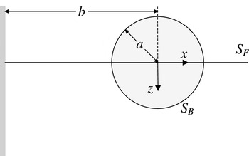
Sketch of the geometry and coordinate system.

2 Formulation
A half-immersed circular cylinder of uniform density, radius
 $a$
and mass
 $M=({\it\rho}{\rm\pi}a^{2})/2$
floats in water of density
 ${\it\rho}$
and with infinite depth; the cylinder is free to move in the plane perpendicular to its axis. Cartesian coordinates
 $(x,y,z)$
are chosen with the origin on the axis of the cylinder,
 $y$
directed parallel to the axis, and
 $z$
directed vertically downwards. A rigid vertical wall is positioned at
 $x=-b$
and the resulting geometry is sketched in figure 1. The cylinder is assumed to be infinitely long and all motions, including those of the water, are assumed to be independent of
 $y$
. The index 1 is used to denote sway motion of the cylinder parallel to the
 $x$
axis, and the index 3 to denote heave motion parallel to the
 $z$
axis. One consequence of the circular geometry is that these are the only modes of motion that can be excited by an incident wave, or by an initial displacement of the structure. The corresponding displacements of the cylinder in the frequency domain are denoted by
 $x_{j}({\it\omega})$
and in the time domain by
 $X_{j}(t)$
,
 $j\in \{1,3\}$
, where
 ${\it\omega}$
is the radian frequency and
 $t$
is time.
2.1 Time-harmonic motion of an isolated cylinder
In this section, required information about the radiation and scattering properties of a cylinder in open water is described. All of the motions discussed in this section are time harmonic with radian frequency
 ${\it\omega}$
and are described by a potential of the form
 $\text{Re}\{{\it\phi}(\boldsymbol{x})\text{e}^{-\text{i}{\it\omega}t}\}$
, where
 ${\it\phi}$
is harmonic within the fluid and satisfies the linearised condition
 $$\begin{eqnarray}\displaystyle K{\it\phi}+\frac{\partial {\it\phi}}{\partial z}=0\quad \text{on }S_{F}, & & \displaystyle\end{eqnarray}$$
where
 $S_{F}$
is the undisturbed free surface,
 $K={\it\omega}^{2}/g$
and
 $g$
is the acceleration due to gravity.
Radiation potentials
 ${\it\phi}_{j}$
,
 $j\in \{1,3\}$
, that describe the forced oscillations of the cylinder with unit velocity amplitude additionally satisfy the boundary conditions
 $$\begin{eqnarray}\displaystyle \frac{\partial {\it\phi}_{j}}{\partial n}=n_{j},\quad j=1,3,\,\text{on}~S_{B}, & & \displaystyle\end{eqnarray}$$
where
 $S_{B}$
is the wetted surface of the cylinder cross-section,
 $n$
is an inward normal coordinate to
 $S_{B}$
, and
 $n_{j}$
is the component of the inward unit normal to
 $S_{B}$
measured parallel to the direction of mode
 $j$
. The sway and heave velocity potentials behave, respectively, as
 $$\begin{eqnarray}\displaystyle {\it\phi}_{1}\sim A_{1}\,\text{e}^{\text{i}K|x|-Kz}\text{sgn}x\quad \text{as }|x|\rightarrow \infty & & \displaystyle\end{eqnarray}$$
and
 $$\begin{eqnarray}\displaystyle {\it\phi}_{3}\sim A_{3}\,\text{e}^{\text{i}K|x|-Kz}\quad \text{as }|x|\rightarrow \infty , & & \displaystyle\end{eqnarray}$$
for some complex constants
 $A_{1}$
and
 $A_{3}$
. Complex-force coefficients for the radiation problems are defined by
 $$\begin{eqnarray}\displaystyle q_{jk}={\it\rho}\int _{S_{B}}{\it\phi}_{j}n_{k}\,\text{d}S,\quad j,k\in \{1,3\}, & & \displaystyle\end{eqnarray}$$
and each such coefficient may be separated into real and imaginary parts by writing
 $q_{jk}={\it\mu}_{jk}+\text{i}{\it\nu}_{jk}$
, where
 ${\it\mu}_{jk}$
is an added-mass coefficient and
 ${\it\omega}{\it\nu}_{jk}$
is a radiation damping coefficient. As
 $S_{B}$
is symmetric about a vertical line by assumption,
 $q_{jk}=0$
for
 $j\neq k$
.
The scattering potential
 ${\it\phi}_{S}$
describes the fluid motion arising when a plane wave of amplitude
 $\mathscr{A}$
is incident from large positive
 $x$
on the fixed cylinder, and is chosen to have the behaviour
 $$\begin{eqnarray}\displaystyle {\it\phi}_{S}\sim \frac{-\text{i}g\mathscr{A}}{{\it\omega}}\left[\text{e}^{-\text{i}Kx-Kz}+R\,\text{e}^{\text{i}Kx-Kz}\right]\quad \text{as }x\rightarrow \infty & & \displaystyle\end{eqnarray}$$
and
 $$\begin{eqnarray}\displaystyle {\it\phi}_{S}\sim \frac{-\text{i}g\mathscr{A}}{{\it\omega}}\left[T\,\text{e}^{-\text{i}Kx-Kz}\right]\quad \text{as }x\rightarrow -\infty , & & \displaystyle\end{eqnarray}$$
where
 $R$
and
 $T$
denote, respectively, the reflection and transmission coefficients. Because of the geometrical symmetry, the reflection and transmission coefficients take the same values for a wave incident from the left. For the wave incident from the right, the exciting force in the direction of mode
 $j$
is defined as
 $$\begin{eqnarray}\displaystyle f_{j}=\text{i}{\it\omega}{\it\rho}\int _{S_{B}}{\it\phi}_{S}n_{j}\,\text{d}S, & & \displaystyle\end{eqnarray}$$
and by the identity
 $$\begin{eqnarray}\displaystyle f_{j}=-\text{i}{\it\rho}g\mathscr{A}A_{j}; & & \displaystyle\end{eqnarray}$$
for further information about this last result see the texts by Linton & McIver (Reference Linton and McIver2001, § 1.4) and Mei, Stiassnie & Yue (Reference Mei, Stiassnie and Yue2005, § 8.6.3).
2.2 The extended wide-spacing approximation
Wide-spacing approximations to the time-harmonic radiation problems for a cylinder in the presence of a wall are given by Porter & Evans (Reference Porter and Evans2011). In these approximations only plane waves are used to determine the interactions between the cylinder and the wall, while the evanescent modes are neglected. Here, the extended wide-spacing approximation developed by McIver (Reference McIver2014) is used to account for the leading-order effects of the evanescent modes in both the radiation and scattering problems. In these approximations it is assumed that both
 ${\it\epsilon}=1/(2Kb)\ll 1$
and
 $a/b\ll 1$
, so that the distance from the wall is large compared to both the wavelength and the cylinder radius. In the case that the wall is present, the complex-force coefficients and the exciting forces are notated by adding a superscript ‘
 $w$
’ to the notation introduced for the isolated cylinder in § 2.1.
The required hydrodynamic quantities from the extended approximation can be conveniently expressed in the same form as the standard wide-spacing approximation that neglects evanescent modes by introducing the notation:
 $$\begin{eqnarray}\displaystyle \hat{R}=R+{\it\epsilon}^{2}p_{3},\quad \hat{T}=T+{\it\epsilon}^{2}p_{3},\quad \hat{A}_{3}=A_{3}\left(1+{\it\epsilon}^{2}{\it\kappa}{\it\sigma}\right), & & \displaystyle\end{eqnarray}$$
 $$\begin{eqnarray}\displaystyle \hat{q}_{33}\equiv \hat{{\it\mu}}_{33}+\text{i}\hat{{\it\nu}}_{33}=q_{33}+2M{\it\epsilon}^{2}{\it\sigma}^{2},\quad \hat{f}_{3}=f_{3}\left(1+{\it\epsilon}^{2}{\it\kappa}{\it\sigma}\right). & & \displaystyle\end{eqnarray}$$
Here
 ${\it\kappa}=Ka$
and, from McIver (Reference McIver2014),
 $p_{3}=-\text{i}{\it\kappa}^{2}A_{3}^{2}/{\rm\pi}a^{2}$
and
 ${\it\sigma}={\it\gamma}_{13}/{\rm\pi}+(1/2){\it\kappa}q_{33}/M$
(
 ${\it\gamma}_{13}$
depends on the geometry of the structure (McIver Reference McIver2014, equation (4.28)), but for the half-immersed circular cylinder
 ${\it\gamma}_{13}=(1/2){\rm\pi}{\it\kappa}-2$
). Note that the results in McIver (Reference McIver2014) are given in terms of complex-force coefficients that are scaled by
 ${\it\rho}a^{2}$
, and exciting forces that are scaled by
 ${\it\rho}ga\mathscr{A}$
. However, in the present work, dimensional coefficients are retained in order to make a direct connection with the results in Porter & Evans (Reference Porter and Evans2011).
The problem of the synchronised heaving of two identical cylinders is treated in McIver (Reference McIver2014) and, by symmetry, half of the heave coefficient calculated there provides the heave force coefficient needed here for a cylinder in the presence of a wall, so that
 $$\begin{eqnarray}\displaystyle q_{33}^{w}=\hat{q}_{33}-\frac{\text{i}{\it\rho}\hat{A}_{3}^{2}}{\text{e}^{-2\text{i}{\it\kappa}b/a}-\hat{R}} & & \displaystyle\end{eqnarray}$$
(note that a factor of two is missing from the last term in (6.18) of McIver (Reference McIver2014)). Other required results are obtained here in appendix A. The remaining complex-force coefficients are
 $$\begin{eqnarray}\displaystyle q_{11}^{w}=q_{11}-\frac{\text{i}{\it\rho}A_{1}^{2}}{\text{e}^{-2\text{i}{\it\kappa}b/a}-\hat{R}} & & \displaystyle\end{eqnarray}$$
and
 $$\begin{eqnarray}\displaystyle q_{13}^{w}=\frac{\text{i}{\it\rho}A_{1}\hat{A}_{3}}{\text{e}^{-2\text{i}{\it\kappa}b/a}-\hat{R}}, & & \displaystyle\end{eqnarray}$$
while the exciting forces are
 $$\begin{eqnarray}\displaystyle f_{1}^{w}=f_{1}\left[1-\frac{\hat{T}}{\text{e}^{-2\text{i}{\it\kappa}b/a}-\hat{R}}\right] & & \displaystyle\end{eqnarray}$$
and
 $$\begin{eqnarray}\displaystyle f_{3}^{w}=\hat{f}_{3}\left[1+\frac{\hat{T}}{\text{e}^{-2\text{i}{\it\kappa}b/a}-\hat{R}}\right]. & & \displaystyle\end{eqnarray}$$
Results given for the standard wide-spacing approximation are recovered by setting
 ${\it\epsilon}$
to zero in (2.10)–(2.11), which is equivalent to dropping the hats in (2.12)–(2.16). When this is done, (2.12)–(2.14) become identical to results given for added-mass and damping coefficients in Porter & Evans (Reference Porter and Evans2011), while, with the aid of (2.9), (2.15)–(2.16) become identical to their equation (3.8).
3 Release from rest of a cylinder in the presence of a wall
3.1 General observations
The first specific problem to be considered is the time-dependent motion that results when the cylinder is displaced vertically a distance
 $z=X_{3}(0)$
and released from rest in calm water. The subsequent time-domain displacements are given by the inverse Fourier transforms
 $$\begin{eqnarray}\displaystyle X_{j}(t)=\frac{1}{2{\rm\pi}}\int _{-\infty +\text{i}v}^{\infty +\text{i}v}x_{j}({\it\omega})\,\text{e}^{-\text{i}{\it\omega}t}\,\text{d}{\it\omega},\quad j\in \{1,3\}, & & \displaystyle\end{eqnarray}$$
where
 $v\in \mathbb{R}$
is, in general, positive to allow for the possibility that a frequency-domain displacement
 $x_{j}({\it\omega})$
may have singularities on the real axis (the absence of motion for
 $t<0$
implies that each
 $x_{j}({\it\omega})$
is analytic in
 $\text{Im}\,{\it\omega}>0$
); see Stakgold (Reference Stakgold2000, § 5.6). In practice, the limit
 ${\it\nu}\rightarrow 0$
is taken on the right-hand side of (3.1). From McIver & McIver (Reference McIver and McIver2011, equation (40))
 $$\begin{eqnarray}\displaystyle x_{1}({\it\omega})=\frac{2\text{i}{\it\rho}ga{\it\omega}^{-1}q_{13}^{w}({\it\omega})X_{3}(0)}{2{\it\rho}ga[M+q_{11}^{w}({\it\omega})]+{\it\omega}^{2}\left\{[q_{13}^{w}({\it\omega})]^{2}-[M+q_{11}^{w}({\it\omega})][M+q_{33}^{w}({\it\omega})]\right\}} & & \displaystyle\end{eqnarray}$$
and
 $$\begin{eqnarray}\displaystyle x_{3}({\it\omega})=\frac{\text{i}{\it\omega}\left\{[q_{13}^{w}({\it\omega})]^{2}-[M+q_{11}^{w}({\it\omega})][M+q_{33}^{w}({\it\omega})]\right\}X_{3}(0)}{2{\it\rho}ga[M+q_{11}^{w}({\it\omega})]+{\it\omega}^{2}\left\{[q_{13}^{w}({\it\omega})]^{2}-[M+q_{11}^{w}({\it\omega})][M+q_{33}^{w}({\it\omega})]\right\}}. & & \displaystyle\end{eqnarray}$$
A matrix formulation of the initial-value problem for floating elastic or rigid structures in two dimensions is given by Meylan (Reference Meylan2014) and the last two results may also be obtained from this. Note that, because of the definition of the Fourier transform, each
 $x_{j}({\it\omega})$
has dimensions of length
 $\times$
time.
In the absence of the trapped modes discovered for this geometry by Porter & Evans (Reference Porter and Evans2009) (and discussed here in § 4), the leading contributions to the large-time asymptotics of the displacements are governed by the behaviour of each
 $x_{j}({\it\omega})$
as
 ${\it\omega}\rightarrow 0$
. In this limit,
 $q_{11}^{w}({\it\omega})$
and
 $q_{13}^{w}({\it\omega})$
have finite non-zero limits while
 $$\begin{eqnarray}\displaystyle q_{33}^{w}({\it\omega})\sim -\frac{32M}{{\rm\pi}^{2}}\log {\it\omega}\quad \text{as }{\it\omega}\rightarrow 0 & & \displaystyle\end{eqnarray}$$
(Porter & Evans Reference Porter and Evans2011, table 1). It follows that
 $$\begin{eqnarray}\displaystyle x_{1}({\it\omega})\sim \frac{\text{i}{\it\mu}_{13}^{w}(0)X_{3}(0)}{{\it\omega}[M+{\it\mu}_{11}^{w}(0)]}\quad \text{as }{\it\omega}\rightarrow 0 & & \displaystyle\end{eqnarray}$$
and
 $$\begin{eqnarray}\displaystyle x_{3}({\it\omega})\sim \frac{8\text{i}aX_{3}(0)}{{\rm\pi}g}\,{\it\omega}\log {\it\omega}\quad \text{as }{\it\omega}\rightarrow 0, & & \displaystyle\end{eqnarray}$$
and hence (McIver & McIver Reference McIver and McIver2011, § 5) that
 $$\begin{eqnarray}\displaystyle X_{1}(t)\rightarrow \frac{{\it\mu}_{13}^{w}(0)X_{3}(0)}{M+{\it\mu}_{11}^{w}(0)}\equiv X_{1}^{\infty }\quad \text{as }t\rightarrow \infty & & \displaystyle\end{eqnarray}$$
and
 $$\begin{eqnarray}\displaystyle X_{3}(t)\sim -\frac{8aX_{3}(0)}{{\rm\pi}gt^{2}}\quad \text{as }t\rightarrow \infty . & & \displaystyle\end{eqnarray}$$
From (3.7), the release of the cylinder from rest results ultimately in a net horizontal translation in a direction that depends upon the sign of the initial vertical displacement (see McIver (Reference McIver2012) for a discussion of circumstances under which a net horizontal translation might occur). From the numerical results in Porter & Evans (Reference Porter and Evans2011),
 ${\it\mu}_{13}^{w}(0)<0$
for a half-immersed cylinder (in fact, a separate numerical solution of the zero-frequency problem gives
 ${\it\mu}_{13}^{w}(0)/M=-0.327$
) so that the net translation is towards the wall when
 $X_{3}(0)>0$
. Equation (3.8) shows that the vertical motion tends to zero algebraically, as found by Ursell (Reference Ursell1964) for the purely vertical motion of a cylinder in open water (Ursell’s result differs from (3.8) by a factor of two due to the presence of the wall in the current work). In fact, (3.8) holds for any two-dimensional structure with a free-surface intersection that is a line of length
 $2a$
.
In addition to the singularities at the origin indicated in (3.5) and (3.6), each
 $x_{j}({\it\omega})$
has poles in the lower half of the complex
 ${\it\omega}$
plane that arise from the zeros of the identical factors in the denominators in (3.2) and (3.3), and hence the poles have identical positions for the horizontal and vertical displacements. Suppose that these poles are at
 ${\it\omega}={\it\omega}_{n}-\text{i}{\it\delta}_{n}$
, with
 $n\in \mathbb{N}\cup \{0\}$
and
 ${\it\omega}_{n},{\it\delta}_{n}\in \mathbb{R}^{+}$
, so that
 $$\begin{eqnarray}\displaystyle x_{j}({\it\omega})\sim \frac{x_{jn}}{{\it\omega}-({\it\omega}_{n}-\text{i}{\it\delta}_{n})}\quad \text{as }{\it\omega}\rightarrow {\it\omega}_{n}-\text{i}{\it\delta}_{n}, & & \displaystyle\end{eqnarray}$$
where
 $x_{jn}$
is the residue at the
 $n$
th pole of
 $x_{j}$
, and
 $\{{\it\omega}_{0},{\it\omega}_{1},\ldots ,{\it\omega}_{n},\ldots \}$
is a monotonically increasing sequence. It follows from a property of the Fourier transform (namely,
 $f(-\overline{{\it\omega}})=\overline{f({\it\omega})}$
for a transform
 $f({\it\omega})$
with
 ${\it\omega}\in \mathbb{C}$
) that the frequency-domain displacements also have a pole at
 ${\it\omega}=-{\it\omega}_{n}-\text{i}{\it\delta}_{n}$
for each
 $n$
, so that
 $$\begin{eqnarray}\displaystyle x_{j}({\it\omega})\sim \frac{-\overline{x_{jn}}}{{\it\omega}+({\it\omega}_{n}+\text{i}{\it\delta}_{n})}\quad \text{as }{\it\omega}\rightarrow -{\it\omega}_{n}-\text{i}{\it\delta}_{n}. & & \displaystyle\end{eqnarray}$$
The contribution of each pair of poles to the behaviour of
 $X_{j}(t)$
is
 $$\begin{eqnarray}\displaystyle 2\,\text{Im}\!\left\{x_{jn}\text{e}^{-\text{i}{\it\omega}_{n}t}\text{e}^{-{\it\delta}_{n}t}\right\}=2|x_{jn}|\sin ({\it\omega}_{n}t-\arg x_{jn}-{\rm\pi})\text{e}^{-{\it\delta}_{n}t} & & \displaystyle\end{eqnarray}$$
(see McIver & McIver Reference McIver and McIver2011, § 5) and, herein, such a motion will be termed a transient. Each transient is a decaying oscillation with an amplitude of twice the modulus of the residue at the relevant pole. In the following, asymptotic methods valid for large
 $n$
are used to approximate each
 ${\it\omega}_{n}$
,
 ${\it\delta}_{n}$
and
 $x_{jn}$
using known high-frequency results for a half-immersed circular cylinder. In fact, later results are given mostly in terms of the complex wavenumber
 ${\it\kappa}={\it\kappa}_{n}+\text{i}{\it\tau}_{n}\equiv ({\it\omega}_{n}-\text{i}{\it\delta}_{n})^{2}a/g$
, so that
 ${\it\kappa}_{n}=({\it\omega}_{n}^{2}-{\it\delta}_{n}^{2})a/g$
and
 ${\it\tau}_{n}=-2{\it\omega}_{n}{\it\delta}_{n}a/g$
.
Numerical results for the magnitudes of the frequency-domain displacements,
 $|x_{1}|$
and
 $|x_{3}|$
, as functions of
 ${\it\kappa}\in \mathbb{R}^{+}$
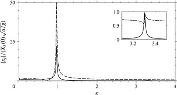
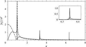
are shown in figure 2 (the required hydrodynamic coefficients were computed using the multipole method described in Porter (Reference Porter2008)). Both displacements show a prominent resonance just below
 ${\it\kappa}=1$
(indexed in this paper by
 $n=0$
) that is a perturbation of that found near
 ${\it\kappa}=0.8$
for the cylinder when in open water (Maskell & Ursell Reference Maskell and Ursell1970). There are also resonances at higher frequencies that are associated with near-standing waves between the cylinder and the wall. For the particular geometry corresponding to figure 2, these resonances occur near
 ${\it\kappa}=n{\rm\pi}$
,
 $n\in \mathbb{N}$
, and are much less prominent than the
 $n=0$
resonance. More detail of the first standing-wave resonance, just above
 ${\it\kappa}={\rm\pi}$
, is shown in the inset to figure 2. One feature of the inset is that, in the case of heave, the perturbation to the curve caused by the resonance is smaller in magnitude than nearby values of the heave displacement itself, which is in agreement with the asymptotic results obtained later in this paper.
The modulus of the scaled frequency-domain displacements
 $|x_{j}|/(X_{3}(0)\sqrt{a/g})$
versus
 ${\it\kappa}$
for a half-immersed cylinder of radius
 $a$
at a distance
 $2a$
from a rigid vertical wall. The solid and dashed lines show, respectively, the sway (
 $j=1$
) and heave (
 $j=3$
) displacements, and the inset shows the resonance near
 ${\it\kappa}=3.3$
in more detail.

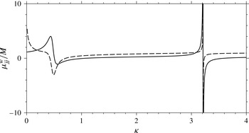
The non-dimensional added masses
 ${\it\mu}_{jj}^{w}/M$
versus
 ${\it\kappa}$
, with
 $j\in \{1,3\}$
, for a half-immersed cylinder of radius
 $a$
at a distance
 $2a$
from a rigid vertical wall. The solid and dashed lines show, respectively, the sway (
 $j=1$
) and heave (
 $j=3$
) values.

There are also resonances in the complex-force coefficients, and it is of particular note that the standing-wave resonances are much more prominent than those in the displacement; one such resonance is shown in figure 3 for the sway and heave added-mass coefficients
 ${\it\mu}_{11}^{w}$
and
 ${\it\mu}_{33}^{w}$
, which may be compared with the corresponding features in figure 2. The literature contains many reported calculations of standing-wave resonances in hydrodynamic coefficients for surface-piercing structures (e.g. Newman Reference Newman1977; Linton & Evans Reference Linton and Evans1992; Yeung & Seah Reference Yeung and Seah2007), and it has been found that, as frequency increases, the resonance peaks in the added-mass and damping coefficients become higher and narrower. It should be noted that, in general, the locations of the resonances of complex-force coefficients
 $q_{jk}^{w}({\it\omega})$
do not coincide with those of the displacements (McIver Reference McIver2005), and a consequence of this is that highly detailed computation of the hydrodynamic coefficients around a resonance may be unnecessary when performing computations of the motion of a freely floating structure. Rather, attention should be paid to the resonances in the displacement which occur at nearby, but distinct, complex frequencies (Lewandowski Reference Lewandowski2008), although it should be noted that the differences in the locations can be quite small.
The main aim now is to use the extended wide-spacing approximations given in § 2.2 to determine approximations to the resonances. Substitution of the approximations (2.12)–(2.14) into (3.2) yields
 $$\begin{eqnarray}\displaystyle x_{1}({\it\omega})=\frac{-2A_{1}\hat{A}_{3}X_{3}(0)}{{\rm\pi}a^{2}{\it\omega}\left[(\text{e}^{-2\text{i}{\it\kappa}b/a}-\hat{R})G_{1}-G_{2}\right]}, & & \displaystyle\end{eqnarray}$$
where
 $$\begin{eqnarray}\displaystyle G_{1}=(1+q_{11}/M)\left(1-{\textstyle \frac{1}{4}}{\rm\pi}{\it\kappa}(1+\hat{q}_{33}/M)\right) & & \displaystyle\end{eqnarray}$$
and
 $$\begin{eqnarray}\displaystyle G_{2}=\frac{2\text{i}}{{\rm\pi}}\left\{\frac{A_{1}^{2}}{a^{2}}-\frac{1}{4}{\rm\pi}{\it\kappa}\left[\left(1+\frac{q_{11}}{M}\right)\frac{\hat{A}_{3}^{2}}{a^{2}}+\left(1+\frac{\hat{q}_{33}}{M}\right)\frac{A_{1}^{2}}{a^{2}}\right]\right\}, & & \displaystyle\end{eqnarray}$$
while substitution of (2.12)–(2.14) into (3.3) gives
 $$\begin{eqnarray}\displaystyle x_{3}({\it\omega}) & = & \displaystyle \frac{\text{i}X_{3}(0)\left[(\text{e}^{-2\text{i}{\it\kappa}b/a}-\hat{R})(G_{1}-(1+q_{11}/M))-(G_{2}-2\text{i}A_{1}^{2}/{\rm\pi}a^{2})\right]}{{\it\omega}\left[(\text{e}^{-2\text{i}{\it\kappa}b/a}-\hat{R})G_{1}-G_{2}\right]},\nonumber\\ \displaystyle & = & \displaystyle \frac{\text{i}X_{3}(0)}{{\it\omega}}\left[\frac{\text{i}{\it\kappa}(1+q_{11}/M)^{2}\hat{A}_{3}^{2}}{2a^{2}G_{1}\left[(\text{e}^{-2\text{i}{\it\kappa}b/a}-\hat{R})G_{1}-G_{2}\right]}-\frac{\frac{1}{4}{\rm\pi}{\it\kappa}(1+\hat{q}_{33}/M)}{1-\frac{1}{4}{\rm\pi}{\it\kappa}(1+\hat{q}_{33}/M)}\right];\qquad\end{eqnarray}$$
the second form for
 $x_{3}$
will be useful later.
3.2 Location of the resonances
The results of the extended wide-spacing approximation are truncated expansions in powers of the small parameter
 ${\it\epsilon}=1/(2Kb)$
(McIver Reference McIver2014), and each expansion coefficient depends upon the non-dimensional wavenumber
 ${\it\kappa}=Ka$
. In the following, each coefficient in the wide-spacing expansion is approximated using asymptotic results for the isolated cylinder valid as
 ${\it\kappa}\rightarrow \infty$
. For the leading term in the wide-spacing approximation a number of terms in the high-frequency expansions will be used in the development of approximations to the resonances. In addition, to give an indication of the significance of evanescent modes, the leading-order effect as
 ${\it\kappa}\rightarrow \infty$
on the resonances will be retained for those terms identified in (2.10) and (2.11) by the explicit appearance of
 ${\it\epsilon}$
. The retention of terms in the high-frequency expansions at the expense of terms in the wide-spacing expansion implicitly assumes that
 ${\it\epsilon}\ll {\it\kappa}^{-1}$
, that is
 $b\gg a$
, which is consistent with one of the wide-spacing assumptions. This section begins by reviewing the required high-frequency results for the half-immersed circular cylinder when in isolation.
The reflection coefficient
 $$\begin{eqnarray}\displaystyle R\sim \text{e}^{-2\text{i}{\it\kappa}}\left[1-\frac{\text{i}}{2{\it\kappa}}+\frac{1}{{\it\kappa}^{2}}\left(-\frac{1}{8}+\frac{2\text{i}}{3{\rm\pi}}\right)+\frac{1}{{\it\kappa}^{3}}\left(\frac{1}{3{\rm\pi}}+\text{i}\,R_{32}\right)\right]\quad \text{as }{\it\kappa}\rightarrow \infty , & & \displaystyle\end{eqnarray}$$
where
 $R_{32}$
is a real number whose value is unknown. This expression up to the term in
 $1/{\it\kappa}$
was obtained by Leppington (Reference Leppington1973), while the term in
 $1/{\it\kappa}^{2}$
is given by Robertson (Reference Robertson1986, table 1). Given the expansion up to
 $1/{\it\kappa}^{2}$
, the real part of the term in
 $1/{\it\kappa}^{3}$
is obtained by ensuring that the energy-flux identity
 $$\begin{eqnarray}\displaystyle |R|^{2}+|T|^{2}=1 & & \displaystyle\end{eqnarray}$$
is consistent with the result
 $$\begin{eqnarray}\displaystyle T & = & \displaystyle \frac{2\text{i}\text{e}^{-2\text{i}{\it\kappa}}}{{\rm\pi}{\it\kappa}^{4}}\left[1+\frac{4}{{\rm\pi}{\it\kappa}}\left({\it\gamma}+\log 2{\it\kappa}-2-\frac{\text{i}{\rm\pi}}{8}\right)\right.\nonumber\\ \displaystyle & & \displaystyle +\,\left.\frac{8\log {\it\kappa}}{{\rm\pi}^{2}{\it\kappa}^{2}}\left(2{\it\gamma}+\log 4{\it\kappa}-5-\frac{\text{i}{\rm\pi}}{4}\right)+O\left(\frac{1}{{\it\kappa}^{2}}\right)\right]\quad \text{as }{\it\kappa}\rightarrow \infty\end{eqnarray}$$
also given by Robertson (Reference Robertson1986), although the leading term was first obtained by Ursell (Reference Ursell1961). (It is not done in Robertson (Reference Robertson1986), and hence not in (3.18) either, but generally in this paper the order notation
 $O\left(1/{\it\kappa}^{n}\right)$
will be used here to include possible terms of the form
 $(\log {\it\kappa})^{m}/{\it\kappa}^{n}$
for integers
 $m\geqslant 0$
.) For the radiation problems, as
 ${\it\kappa}\rightarrow \infty$
 $$\begin{eqnarray}\displaystyle A_{1}\sim -\frac{2\text{i}a\,\text{e}^{-\text{i}{\it\kappa}}}{{\it\kappa}}\left[1+\frac{2}{{\rm\pi}{\it\kappa}}\left({\it\gamma}+\log 2{\it\kappa}-2-\frac{\text{i}{\rm\pi}}{8}\right)\right], & & \displaystyle\end{eqnarray}$$
 $$\begin{eqnarray}\displaystyle A_{3}\sim -\frac{4\text{i}a\,\text{e}^{-\text{i}{\it\kappa}}}{{\it\kappa}^{2}}\left[1+\frac{2}{{\rm\pi}{\it\kappa}}\left({\it\gamma}+\log 2{\it\kappa}-3-\frac{\text{i}{\rm\pi}}{8}\right)\right], & & \displaystyle\end{eqnarray}$$
 $$\begin{eqnarray}\displaystyle \frac{{\it\mu}_{11}}{M}\sim \frac{4}{{\rm\pi}^{2}}-\frac{0.73789}{{\it\kappa}},\quad \frac{{\it\nu}_{11}}{M}\sim \frac{8}{{\rm\pi}{\it\kappa}^{2}}\left[1+\frac{4}{{\rm\pi}{\it\kappa}}({\it\gamma}+\log 2{\it\kappa}-2)\right], & & \displaystyle\end{eqnarray}$$
 $$\begin{eqnarray}\displaystyle \frac{{\it\mu}_{33}}{M}\sim 1-\frac{4}{3{\rm\pi}{\it\kappa}}-\frac{2}{{\it\kappa}^{2}}\left(1-\frac{8}{{\rm\pi}^{2}}\right),\quad \frac{{\it\nu}_{33}}{M}\sim \frac{32}{{\rm\pi}{\it\kappa}^{4}}\left[1+\frac{4}{{\rm\pi}{\it\kappa}}({\it\gamma}+\log 2{\it\kappa}-3)\right].\qquad \quad & & \displaystyle\end{eqnarray}$$
The expressions for
 $A_{1}$
,
 $A_{3}$
,
 ${\it\mu}_{33}$
and the leading-order term for
 ${\it\mu}_{11}$
are given by Simon (Reference Simon1985). The numerical coefficient in the expansion of
 ${\it\mu}_{11}$
was calculated by Greenhow (Reference Greenhow1986, equation (27)), while the expressions for the damping coefficients
 ${\it\nu}_{11}$
and
 ${\it\nu}_{33}$
are obtained from Simon’s results with the help of a known relation between damping coefficients and radiated wave amplitudes (Linton & McIver Reference Linton and McIver2001, equation (1.52)).
The resonances of the displacements given in (3.12) and (3.15) occur at the solutions for
 ${\it\kappa}$
of
 $$\begin{eqnarray}\displaystyle \text{e}^{-2\text{i}{\it\kappa}b/a+2n{\rm\pi}\text{i}}=\hat{R}+\frac{G_{2}}{G_{1}}\equiv \hat{R}(1+S), & & \displaystyle\end{eqnarray}$$
where
 $n\in \mathbb{N}$
is chosen,
 $S=G_{2}/G_{1}\hat{R}$
and
 $$\begin{eqnarray}\displaystyle \frac{G_{2}}{G_{1}}=\frac{2\text{i}}{{\rm\pi}a^{2}}\left[\frac{A_{1}^{2}}{1+q_{11}/M}-\frac{\frac{1}{4}{\rm\pi}{\it\kappa}\hat{A}_{3}^{2}}{1-\frac{1}{4}{\rm\pi}{\it\kappa}(1+\hat{q}_{33}/M)}\right]. & & \displaystyle\end{eqnarray}$$
From this form, and the asymptotics in (3.19)–(3.22), it may be seen that at high frequencies the sway characteristics of the cylinder have a stronger influence on the locations of the resonances than the heave characteristics. This is physically reasonable because, as a result of the vertical free-surface intersections, a surging cylinder generates larger waves at high frequencies than a cylinder heaving with the same amplitude, and hence the surging cylinder interacts more strongly with the wall.
Suppose that a resonance, indexed by the integer
 $n$
, occurs at
 ${\it\kappa}={\it\kappa}_{n}+\text{i}{\it\tau}_{n}$
, where
 ${\it\kappa}_{n},{\it\tau}_{n}\in \mathbb{R}$
and
 $|{\it\tau}_{n}|\ll |{\it\kappa}_{n}|$
. The modified reflection coefficient
 $\hat{R}$
may be extended into the complex
 ${\it\kappa}$
plane within a neighbourhood of
 ${\it\kappa}_{n}$
(McIver Reference McIver2005), and then by Taylor series expansion
 $$\begin{eqnarray}\displaystyle \hat{R}({\it\kappa})=\hat{R}({\it\kappa}_{n})+\text{i}{\it\tau}_{n}\hat{R}^{\prime }({\it\kappa}_{n})+O({\it\tau}_{n}^{2})\quad \text{as }{\it\tau}_{n}\rightarrow 0, & & \displaystyle\end{eqnarray}$$
where, by a property of functions of a complex variable, the derivative
 $\hat{R}^{\prime }$
may be taken along the real axis (this idea is also used in Meylan & Tomic (Reference Meylan and Tomic2012, § 3) for the calculation of resonances). A similar expression holds for
 $S$
and hence, from (3.23),
 $$\begin{eqnarray}\displaystyle -\frac{2\text{i}b}{a}({\it\kappa}_{n}+\text{i}{\it\tau}_{n})+2n{\rm\pi}\text{i}=\log [\hat{R}(1+S)]+\frac{\text{i}{\it\tau}_{n}\hat{R}^{\prime }}{\hat{R}}+\frac{\text{i}{\it\tau}_{n}S^{\prime }}{1+S}+O({\it\tau}_{n}^{2}), & & \displaystyle\end{eqnarray}$$
where
 $\hat{R}$
,
 $S$
and their derivatives are now evaluated at
 ${\it\kappa}={\it\kappa}_{n}$
.
The real part of (3.26) yields
 $$\begin{eqnarray}\displaystyle \frac{2b{\it\tau}_{n}}{a}=\log |R|+{\it\epsilon}^{2}\,\text{Re}\,\frac{p_{3}}{R}+\log |1+S|-{\it\tau}_{n}\,\text{Im}\!\left\{\frac{\hat{R}^{\prime }}{\hat{R}}+\frac{S^{\prime }}{1+S}\right\}+O({\it\tau}_{n}^{2},{\it\epsilon}^{4}). & & \displaystyle\end{eqnarray}$$
From (3.17) and (3.18), as
 ${\it\kappa}\rightarrow \infty$
 $$\begin{eqnarray}\displaystyle \log |R|=\frac{1}{2}\log (1-|T|^{2})\sim -\frac{2}{{\rm\pi}^{2}{\it\kappa}^{8}}, & & \displaystyle\end{eqnarray}$$
and from results in appendix B
 $$\begin{eqnarray}\displaystyle {\it\epsilon}^{2}\,\text{Re}\,\frac{p_{3}}{R}\sim -\frac{8a^{2}}{{\rm\pi}^{2}b^{2}{\it\kappa}^{8}},\quad \log |1+S|\sim -\frac{32{\rm\pi}^{2}}{\left(4+{\rm\pi}^{2}\right)^{2}{\it\kappa}^{4}}, & & \displaystyle\end{eqnarray}$$
 $$\begin{eqnarray}\displaystyle \text{Im}\!\left\{\frac{\hat{R}^{\prime }}{\hat{R}}\right\}\sim -2\quad \text{and}\quad \text{Im}\!\left\{\frac{S^{\prime }}{1+S}\right\}\sim \frac{16{\rm\pi}}{\left(4+{\rm\pi}^{2}\right){\it\kappa}^{3}}, & & \displaystyle\end{eqnarray}$$
so that
 $$\begin{eqnarray}\displaystyle {\it\tau}_{n}\sim -\frac{16{\rm\pi}^{2}}{(b/a-1)\left(4+{\rm\pi}^{2}\right)^{2}{\it\kappa}_{n}^{4}}\quad \text{as }{\it\kappa}_{n}\rightarrow \infty . & & \displaystyle\end{eqnarray}$$
The imaginary part of (3.26) yields
 $$\begin{eqnarray}\displaystyle & \displaystyle -\frac{2b{\it\kappa}_{n}}{a}+2n{\rm\pi}=\arg R+{\it\epsilon}^{2}\,\text{Im}\,\frac{p_{3}}{R}+\arg (1+S)+{\it\tau}_{n}\,\text{Re}\!\left\{\frac{\hat{R}^{\prime }}{\hat{R}}+\frac{S^{\prime }}{1+S}\right\}+O({\it\tau}_{n}^{2},{\it\epsilon}^{4}). & \displaystyle \nonumber\\ \displaystyle & & \displaystyle\end{eqnarray}$$
From (3.16), as
 ${\it\kappa}\rightarrow \infty$
 $$\begin{eqnarray}\displaystyle \arg R\sim -2{\it\kappa}-\frac{1}{2{\it\kappa}}+\frac{2}{3{\rm\pi}{\it\kappa}^{2}} & & \displaystyle\end{eqnarray}$$
and from results in appendix B
 $$\begin{eqnarray}\displaystyle {\it\epsilon}^{2}\,\text{Im}\,\frac{p_{3}}{R}\sim \frac{4a^{2}}{{\rm\pi}b^{2}{\it\kappa}^{4}},\quad \arg (1+S)\sim -\frac{8{\rm\pi}}{(4+{\rm\pi}^{2}){\it\kappa}^{2}}, & & \displaystyle\end{eqnarray}$$
 $$\begin{eqnarray}\displaystyle \text{Re}\!\left\{\frac{\hat{R}^{\prime }}{\hat{R}}\right\}=o\left(\frac{1}{{\it\kappa}^{3}}\right)\quad \text{and}\quad \text{Re}\!\left\{\frac{S^{\prime }}{1+S}\right\}=o\left(\frac{1}{{\it\kappa}^{3}}\right). & & \displaystyle\end{eqnarray}$$
Hence
 $$\begin{eqnarray}\displaystyle {\it\kappa}_{n}(b/a-1)\sim n{\rm\pi}+\frac{1}{4{\it\kappa}_{n}}-\frac{1}{3{\rm\pi}{\it\kappa}_{n}^{2}}\left(1-\frac{12{\rm\pi}^{2}}{4+{\rm\pi}^{2}}\right)\quad \text{as }{\it\kappa}_{n}\rightarrow \infty & & \displaystyle\end{eqnarray}$$
and reversion gives
 $$\begin{eqnarray}\displaystyle {\it\kappa}_{n}\sim \frac{n{\rm\pi}}{b/a-1}+\frac{1}{4n{\rm\pi}}-\frac{b/a-1}{3n^{2}{\rm\pi}^{3}}\left(1-\frac{12{\rm\pi}^{2}}{4+{\rm\pi}^{2}}\right)\quad \text{as }n\rightarrow \infty . & & \displaystyle\end{eqnarray}$$
The first approximation from (3.37) in (3.31) yields
 $$\begin{eqnarray}\displaystyle {\it\tau}_{n}\sim -\frac{16(b/a-1)^{3}}{\left(4+{\rm\pi}^{2}\right)^{2}{\rm\pi}^{2}n^{4}}\quad \text{as }n\rightarrow \infty . & & \displaystyle\end{eqnarray}$$
To the order given above, the above approximations to
 ${\it\kappa}_{n}$
and
 ${\it\tau}_{n}$
contain no contributions from the evanescent modes that are included in the extended wide-spacing approximation, so that, to the order given, such modes have no influence on the locations of the displacement resonances.
The resonances of the hydrodynamic coefficients in (2.12)–(2.14) occur at the solutions for
 ${\it\kappa}$
of
 $$\begin{eqnarray}\displaystyle \text{e}^{-2\text{i}{\it\kappa}b/a+2n{\rm\pi}\text{i}}=\hat{R} & & \displaystyle\end{eqnarray}$$
and hence may be recovered by setting
 $S=0$
in the above calculations. In a similar fashion to the above, suppose that a resonance, indexed by the integer
 $n$
, occurs at
 ${\it\kappa}={\it\kappa}_{q,n}+\text{i}{\it\tau}_{q,n}$
, where
 ${\it\kappa}_{q,n},{\it\tau}_{q,n}\in \mathbb{R}$
and
 $|{\it\tau}_{q,n}|\ll |{\it\kappa}_{q,n}|$
. Equation (3.27) with
 $S=0$
yields
 $$\begin{eqnarray}\displaystyle {\it\tau}_{q,n}\sim -\frac{1+4a^{2}/b^{2}}{(b/a-1){\rm\pi}^{2}{\it\kappa}_{q,n}^{8}}\quad \text{as }{\it\kappa}_{q,n}\rightarrow \infty & & \displaystyle\end{eqnarray}$$
so that for each high-frequency resonance
 $|{\it\tau}_{q,n}|\ll |{\it\tau}_{n}|$
. The term in
 $a^{2}/b^{2}$
in the expression for
 ${\it\tau}_{q,n}$
arises from evanescent terms in the extended wide-spacing approximation. Equation (3.32) with
 $S=0$
gives
 $$\begin{eqnarray}\displaystyle {\it\kappa}_{q,n}\sim \frac{n{\rm\pi}}{b/a-1}+\frac{1}{4n{\rm\pi}}-\frac{b/a-1}{3n^{2}{\rm\pi}^{3}}\quad \text{as }n\rightarrow \infty & & \displaystyle\end{eqnarray}$$
and then the first approximation from (3.41) in (3.40) yields
 $$\begin{eqnarray}\displaystyle {\it\tau}_{q,n}\sim -\frac{(1+4a^{2}/b^{2})(b/a-1)^{7}}{{\rm\pi}^{10}n^{8}}\quad \text{as }n\rightarrow \infty . & & \displaystyle\end{eqnarray}$$
The results in (3.37) and (3.41) reveal a positive shift in the real part of a displacement resonance frequency relative to the corresponding value for the hydrodynamic coefficients (such shifts in a resonance are discussed in McIver (Reference McIver2005)).


From the leading-order approximations
 ${\it\kappa}_{n}\approx {\it\kappa}_{q,n}\approx n{\rm\pi}/(b/a-1)$
it is apparent that the validity of this procedure depends upon the spacing
 $b/a$
as well as the mode number
 $n$
. As
 $b/a$
increases, the real parts of the resonance locations decrease, and hence these high-frequency approximations cannot be expected to work well for small
 $n$
when
 $b/a$
is large. On the other hand, when
 $b/a$
takes a modest value, say less than approximately two, all standing-wave resonances can be thought of as lying in the high-frequency regime. Although the validity of the wide-spacing approximation might then be questioned, there is much published work to suggest that it performs well even when the basic assumptions are violated. This view is supported by the results in table 1 which, for
 $b/a=2$
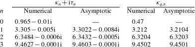
, compare the asymptotic approximations to the displacement resonances given in (3.37) and (3.38), and the real parts of the resonances in the hydrodynamic coefficients (3.41) (the imaginary parts are very small), with numerical estimates obtained using the method described in Fitzgerald & McIver (Reference Fitzgerald and McIver2009). The lowest resonances (
 $n=0$
) are not revealed by the asymptotic method, as the above procedure relies on the poles being both close to the real frequency axis and within the high-frequency regime. The distance from the real axis also makes an
 $n=0$
resonance more difficult to locate accurately from the numerical results. However, for the geometry chosen here, for
 $n\geqslant 1$
the accuracy of the approximations is good even for small
 $n$
.
3.3 Residues
The residues at simple poles of
 $x_{j}$
in the complex plane are estimated as follows. Suppose that
 $$\begin{eqnarray}\displaystyle x_{j}({\it\omega})=\frac{f_{j}({\it\kappa}({\it\omega}))}{h({\it\kappa}({\it\omega}))}, & & \displaystyle\end{eqnarray}$$
where
 ${\it\kappa}({\it\omega})={\it\omega}^{2}a/g$
, and
 $h({\it\kappa})$
has a simple zero at
 ${\it\kappa}=\widetilde{{\it\kappa}}\equiv \widetilde{{\it\omega}}^{2}a/g$
so that
 $h(\widetilde{{\it\kappa}})=0$
,
 $h^{\prime }(\widetilde{{\it\kappa}})\neq 0$
and
 $f_{j}(\widetilde{{\it\kappa}})\neq 0$
(here
 $\widetilde{{\it\omega}}$
is complex and has positive real part – see § 3.1). When
 $x_{j}$
is regarded as a function of
 ${\it\kappa}$
, so that
 $$\begin{eqnarray}\displaystyle x_{j}\sim \frac{x_{jn}^{({\it\kappa})}}{{\it\kappa}-\widetilde{{\it\kappa}}}\quad \text{as }{\it\kappa}\rightarrow \widetilde{{\it\kappa}}\equiv {\it\kappa}_{n}+\text{i}{\it\tau}_{n}, & & \displaystyle\end{eqnarray}$$
then the residue
 $$\begin{eqnarray}\displaystyle x_{jn}^{({\it\kappa})}=\lim _{{\it\kappa}\rightarrow \widetilde{{\it\kappa}}}\frac{({\it\kappa}-\widetilde{{\it\kappa}})f_{j}({\it\kappa})}{h({\it\kappa})}=\frac{f_{j}(\widetilde{{\it\kappa}})}{h^{\prime }(\widetilde{{\it\kappa}})}\sim \frac{f_{j}({\it\kappa}_{n})}{h^{\prime }({\it\kappa}_{n})}\quad \text{as }{\it\tau}_{n}\rightarrow 0. & & \displaystyle\end{eqnarray}$$
When
 $x_{j}$
is regarded as a function of
 ${\it\omega}$
, so that (3.9) holds, then the residue
 $$\begin{eqnarray}\displaystyle & \displaystyle x_{jn}=\lim _{{\it\omega}\rightarrow \widetilde{{\it\omega}}}\frac{({\it\omega}-\widetilde{{\it\omega}})f_{j}({\it\kappa}({\it\omega}))}{h({\it\kappa}({\it\omega}))}=\lim _{{\it\kappa}\rightarrow \widetilde{{\it\kappa}}}\frac{({\it\kappa}-\widetilde{{\it\kappa}})}{2\widetilde{{\it\omega}}a/g}\frac{f_{j}({\it\kappa})}{h({\it\kappa})}=\frac{x_{jn}^{({\it\kappa})}}{(2\widetilde{{\it\omega}}a/g)}\sim \frac{x_{jn}^{({\it\kappa})}}{(2{\it\omega}_{n}a/g)}\quad \text{as }{\it\tau}_{n}\rightarrow 0, & \displaystyle \nonumber\\ \displaystyle & & \displaystyle\end{eqnarray}$$
where the positive real number
 ${\it\omega}_{n}=\sqrt{g{\it\kappa}_{n}/a}$
.
With
 $$\begin{eqnarray}\displaystyle h({\it\kappa})=\text{e}^{-2\text{i}{\it\kappa}b/a}-\hat{R}-G_{2}/G_{1} & & \displaystyle\end{eqnarray}$$
then, as
 ${\it\kappa}\rightarrow \infty$
,
 $$\begin{eqnarray}\displaystyle h^{\prime }({\it\kappa}) & = & \displaystyle -\frac{2\text{i}b}{a}\text{e}^{-2\text{i}{\it\kappa}b/a}+2\text{i}\text{e}^{-2\text{i}{\it\kappa}}\left[1+O\left({\it\kappa}^{-1}\right)\right]\nonumber\\ \displaystyle & = & \displaystyle -2\text{i}\text{e}^{-2\text{i}{\it\kappa}}\left[\frac{b}{a}\,\text{e}^{-2\text{i}{\it\kappa}(b/a-1)}-1+O\left({\it\kappa}^{-1}\right)\right],\end{eqnarray}$$
so that
 $$\begin{eqnarray}\displaystyle h^{\prime }({\it\kappa}_{n})=-2\text{i}\text{e}^{-2\text{i}{\it\kappa}_{n}}\left[b/a-1+O\left(1/n\right)\right]\quad \text{as }n\rightarrow \infty . & & \displaystyle\end{eqnarray}$$
As
 ${\it\kappa}\rightarrow \infty$
 $$\begin{eqnarray}\displaystyle \frac{\hat{A}_{3}}{aG_{1}} & = & \displaystyle \frac{(A_{3}/a)(1+{\it\epsilon}^{2}{\it\kappa}{\it\sigma})}{(1+q_{11}/M)(1-\frac{1}{4}{\rm\pi}{\it\kappa}(1+q_{33}/M+2{\it\epsilon}^{2}{\it\sigma}^{2}))}\nonumber\\ \displaystyle & {\sim} & \displaystyle \frac{(A_{3}/a)(1+a^{2}/4b^{2})}{-\frac{1}{4}{\rm\pi}{\it\kappa}(1+q_{11}/M)(1+q_{33}/M+a^{2}/2b^{2})}\sim \frac{8{\rm\pi}\text{i}\text{e}^{-\text{i}{\it\kappa}}}{(4+{\rm\pi}^{2}){\it\kappa}^{3}},\end{eqnarray}$$
so that, to leading order in
 ${\it\kappa}$
, the contributions from the evanescent terms (identified by
 $a^{2}/b^{2}$
) to
 $\hat{A}_{3}$
and
 $G_{1}$
cancel. From (3.12), for the horizontal displacement
 $$\begin{eqnarray}\displaystyle f_{1}({\it\kappa})=\frac{-2A_{1}\hat{A}_{3}X_{3}(0)}{{\rm\pi}a^{2}{\it\omega}G_{1}}\sim -\frac{32\text{e}^{-2\text{i}{\it\kappa}}X_{3}(0)}{{\it\omega}(4+{\rm\pi}^{2}){\it\kappa}^{4}}\quad \text{as }{\it\kappa}\rightarrow \infty & & \displaystyle\end{eqnarray}$$
so that from (3.45) and (3.46) the residue
 $$\begin{eqnarray}\displaystyle x_{1n}\sim \frac{-8\text{i}X_{3}(0)}{(b/a-1)(4+{\rm\pi}^{2}){\it\kappa}_{n}^{5}}\sim \frac{-8\text{i}(b/a-1)^{4}X_{3}(0)}{(4+{\rm\pi}^{2}){\rm\pi}^{5}n^{5}}\quad \text{as }n\rightarrow \infty . & & \displaystyle\end{eqnarray}$$
From the second form for the vertical displacement in (3.15), the term that is singular at resonance gives
 $$\begin{eqnarray}\displaystyle f_{3}({\it\kappa})=-\frac{{\it\kappa}X_{3}(0)}{2{\it\omega}}\left[\left(1+\frac{q_{11}}{M}\right)\frac{\hat{A}_{3}}{aG_{1}}\right]^{2}\sim \frac{32\text{e}^{-2\text{i}{\it\kappa}}X_{3}(0)}{{\it\omega}{\rm\pi}^{2}{\it\kappa}^{5}}\quad \text{as }{\it\kappa}\rightarrow \infty & & \displaystyle\end{eqnarray}$$
and hence the residue
 $$\begin{eqnarray}\displaystyle x_{3n}\sim \frac{8\text{i}X_{3}(0)}{(b/a-1){\rm\pi}^{2}{\it\kappa}_{n}^{6}}\sim \frac{8\text{i}(b/a-1)^{5}X_{3}(0)}{{\rm\pi}^{8}n^{6}}\quad \text{as }n\rightarrow \infty & & \displaystyle\end{eqnarray}$$
so that the amplitude of a vertical transient is asymptotically an order of magnitude smaller than the corresponding horizontal transient, although both decay very rapidly with increasing
 $n$
.
For real
 ${\it\kappa}$
near a resonance at
 ${\it\kappa}_{n}+\text{i}{\it\tau}_{n}$
, the magnitude of the contribution to
 $x_{j}$
, when regarded as a function of
 ${\it\kappa}$
, from that resonance is
 $|x_{jn}^{({\it\kappa})}|/\sqrt{({\it\kappa}-{\it\kappa}_{n})^{2}+{\it\tau}_{n}^{2}}$
. This is greatest at
 ${\it\kappa}={\it\kappa}_{n}$
, and as
 $n\rightarrow \infty$
the maximum value is
 $$\begin{eqnarray}\displaystyle \frac{|x_{jn}^{({\it\kappa})}|}{|{\it\tau}_{n}|}\sim \frac{2{\it\omega}_{n}a}{g}\frac{|x_{jn}|}{|{\it\tau}_{n}|}\sim \left\{\begin{array}{@{}ll@{}}\displaystyle \left|X_{3}(0)\right|\sqrt{\frac{a}{g}}\,\frac{(4+{\rm\pi}^{2})}{{\rm\pi}^{2}{\it\kappa}_{n}^{1/2}},\quad & j=1;\\ \displaystyle \left|X_{3}(0)\right|\sqrt{\frac{a}{g}}\,\frac{(4+{\rm\pi}^{2})^{2}}{{\rm\pi}^{4}{\it\kappa}_{n}^{3/2}},\quad & j=3,\end{array}\right. & & \displaystyle\end{eqnarray}$$
with
 ${\it\kappa}_{n}\sim n{\rm\pi}/(b/a-1)$
. The powers of
 ${\it\kappa}_{n}$
in these expressions indicate that the contribution to the displacement from a particular resonance is smaller for heave, which confirms the behaviour seen in the numerical results given in the inset to figure 2.
3.4 High-frequency asymptotics away from resonance
Away from the resonances, so that
 $\text{e}^{-2\text{i}{\it\kappa}b/a}-R=\text{ord}\left(1\right)$
as
 ${\it\kappa}\rightarrow \infty$
through suitable values (
 $\text{ord}\left(1\right)$
denotes ‘strictly order one’ (Hinch Reference Hinch1991, p. 6)), the leading-order approximation to the denominator in (3.12) arises from the term in
 $G_{1}$
to give
 $$\begin{eqnarray}\displaystyle x_{1}({\it\omega})\sim \frac{16X_{3}(0)}{{\it\omega}(4+{\rm\pi}^{2}){\it\kappa}^{4}}\left[1-\text{i}\cot {\it\kappa}(b/a-1)\right]\quad \text{as }{\it\omega}\rightarrow \infty & & \displaystyle\end{eqnarray}$$
so that, to leading order, and unlike the imaginary part,
 $\text{Re}\,x_{1}({\it\omega})$
decays monotonically with increasing frequency. Similarly, from (3.15),
 $$\begin{eqnarray}\displaystyle & \displaystyle x_{3}({\it\omega})+\frac{\text{i}X_{3}(0)}{{\it\omega}}\frac{\frac{1}{4}{\rm\pi}{\it\kappa}(1+\hat{q}_{33}/M)}{1-\frac{1}{4}{\rm\pi}{\it\kappa}(1+\hat{q}_{33}/M)}\sim -\frac{16X_{3}(0)}{{\it\omega}{\rm\pi}^{2}{\it\kappa}^{5}}\left[1-\text{i}\cot {\it\kappa}(b/a-1)\right]\quad \text{as }{\it\omega}\rightarrow \infty & \displaystyle \nonumber\\ \displaystyle & & \displaystyle\end{eqnarray}$$
(the asymptotics of
 $\hat{q}_{33}$
are not known in sufficient detail to allow the imaginary part of the second term on the left-hand side to be expanded to the same order as the term on the right – more information about the real part is given below). These results confirm one of the features shown in figure 2, namely that the general trend with increasing frequency is for the sway displacement to decrease more rapidly than the heave displacement. As
 $$\begin{eqnarray}\displaystyle \cot {\it\kappa}(b/a-1)\sim \frac{1}{(b/a-1)({\it\kappa}-\widehat{{\it\kappa}})}\quad \text{as }{\it\kappa}\rightarrow \widehat{{\it\kappa}}\equiv \frac{n{\rm\pi}}{b/a-1} & & \displaystyle\end{eqnarray}$$
the residues in (3.52) and (3.54) are recovered once account has been taken of (3.46). The above expressions confirm that the imaginary parts of the frequency-domain displacements are most strongly influenced by the resonances.
The imaginary part of the vertical displacement decays particularly slowly with increasing frequency as
 $$\begin{eqnarray}\displaystyle x_{3}({\it\omega})\sim \frac{\text{i}X_{3}(0)}{{\it\omega}}\quad \text{as }{\it\omega}\rightarrow \infty & & \displaystyle\end{eqnarray}$$
(by a result on Fourier transforms (Bleistein & Handelsman Reference Bleistein and Handelsman1986, p. 80), (3.59) is effectively a restatement of the initial condition on
 $X_{3}(t)$
). Further expansion in (3.57) yields
 $$\begin{eqnarray}\displaystyle \text{Re}\,x_{3}({\it\omega})\sim \frac{16X_{3}(0)}{{\it\omega}{\rm\pi}^{2}{\it\kappa}^{5}}\left[\frac{2(1+a^{2}/2b^{2})}{(1+a^{2}/4b^{2})^{2}}-1\right]\quad \text{as }{\it\omega}\rightarrow \infty & & \displaystyle\end{eqnarray}$$
which decays with increasing frequency much more quickly than
 $\text{Im}\,x_{3}({\it\omega})$
. While (3.59) holds for a cylinder in open water, the limit
 $b/a\rightarrow \infty$
in (3.60) does not recover the open-water result for the real part, as interactions with the wall through propagating waves are present for any
 $b/a>1$
; in fact, for open water,
 $$\begin{eqnarray}\displaystyle \text{Re}\,x_{3}({\it\omega})\sim \frac{32X_{3}(0)}{{\it\omega}{\rm\pi}^{2}{\it\kappa}^{5}}\quad \text{as }{\it\omega}\rightarrow \infty . & & \displaystyle\end{eqnarray}$$
3.5 Computation of the displacements
The time-domain displacements
 $X_{j}(t)$
are recovered from the frequency-domain displacements
 $x_{j}({\it\omega})$
through the inverse Fourier transform (3.1). In § 3.1 it is noted that
 $x_{1}({\it\omega})$
has a simple pole at the origin, leading to a non-zero large-time displacement
 $X_{1}^{\infty }$
given by (3.7). It is also possible that, for the chosen value of
 $a/b$
, there may be simple poles at
 ${\it\omega}={\it\omega}_{0}$
with
 ${\it\omega}_{0}\in \mathbb{R}^{+}$
corresponding to the existence of a trapped mode (equations (3.9) and (3.10) with
 $n=0$
and
 ${\it\delta}_{0}=0$
give the asymptotic behaviours at such poles); the existence of trapped modes for
 $a/b=0.22504,0.60333$
is established numerically in Porter & Evans (Reference Porter and Evans2009). Frequency-domain quantities with these poles extracted are
 $$\begin{eqnarray}\displaystyle y_{j}({\it\omega})=x_{j}({\it\omega})-\frac{\text{i}X_{j}^{\infty }}{{\it\omega}}-\frac{x_{j0}}{{\it\omega}-{\it\omega}_{0}}+\frac{\overline{x_{j0}}}{{\it\omega}+{\it\omega}_{0}},\quad j\in \{1,3\}, & & \displaystyle\end{eqnarray}$$
where, to unify the notation,
 $X_{3}^{\infty }=0$
. As each
 $y_{j}({\it\omega})$
is now free of singularities in
 $\text{Im}\,{\it\omega}\geqslant 0$
, it follows from (3.1) that
 $$\begin{eqnarray}\displaystyle X_{j}(t)=\frac{1}{2{\rm\pi}}\int _{-\infty }^{\infty }y_{j}({\it\omega})\text{e}^{-\text{i}{\it\omega}t}\,\text{d}{\it\omega}+X_{j}^{\infty }+2\,\text{Im}\{x_{j0}\text{e}^{-\text{i}{\it\omega}_{0}t}\},\quad t>0, & & \displaystyle\end{eqnarray}$$
where the integration is now taken along the real
 ${\it\omega}$
axis and the pole contributions are obtained by closing the contour in the lower half-plane. Further, as noted by Meylan (Reference Meylan2014, § 3) (see also McIver Reference McIver2012, appendix A), by virtue of the analytic properties of
 $y_{j}({\it\omega})$
in the upper half-plane, the inverse Fourier transform of
 $y_{j}({\it\omega})$
may be rewritten either in terms of the cosine transform of the real part of
 $y_{j}({\it\omega})$
or the sine transform of the imaginary part of
 $y_{j}({\it\omega})$
. From the high-frequency results in (3.56) and (3.59)–(3.60), it is apparent that the real parts of the frequency-domain displacements are better suited to computations, and hence it is appropriate to use
 $$\begin{eqnarray}\displaystyle X_{j}(t)=\frac{2}{{\rm\pi}}\int _{0}^{\infty }\,\text{Re}\{y_{j}({\it\omega})\}\cos {\it\omega}t\,\text{d}{\it\omega}+X_{j}^{\infty }+2\,\text{Im}\{x_{j0}\text{e}^{-\text{i}{\it\omega}_{0}t}\},\quad t>0. & & \displaystyle\end{eqnarray}$$
For
 $x_{j0}\neq 0$
, the initial conditions determine each
 $x_{j0}$
. As both
 $\text{Re}\{y_{j}({\it\omega})\}$
and
 ${\it\omega}\,\text{Re}\{y_{j}({\it\omega})\}$
are absolutely integrable over
 $(0,\infty )$
, the limit
 $t\rightarrow 0$
may be taken under the integral sign in both the integral term in
 $X_{j}(t)$
and its first derivative with respect to
 $t$
. The velocity conditions
 ${\dot{X}}_{1}(0)={\dot{X}}_{3}(0)=0$
yield that the real part of each
 $x_{j0}$
is zero so that, in fact,
 $\text{Re}\{y_{j}({\it\omega})\}=\text{Re}\{x_{j}({\it\omega})\}$
. The conditions on the initial displacements then give
 $$\begin{eqnarray}\displaystyle \text{Im}\{x_{j0}\}=\frac{1}{2}\left[X_{j}(0)-\frac{2}{{\rm\pi}}\int _{0}^{\infty }\,\text{Re}\{x_{j}({\it\omega})\}\,\text{d}{\it\omega}-X_{j}^{\infty }\right], & & \displaystyle\end{eqnarray}$$
which determines the amplitude of the trapped mode, and hence
 $$\begin{eqnarray}\displaystyle X_{j}(t)=\frac{2}{{\rm\pi}}\int _{0}^{\infty }\,\text{Re}\{x_{j}({\it\omega})\}\cos {\it\omega}t\,\text{d}{\it\omega}+X_{j}^{\infty }+2\,\text{Im}\{x_{j0}\}\cos {\it\omega}_{0}t,\quad t>0. & & \displaystyle\end{eqnarray}$$
In the absence of a trapped mode no special treatment of the initial condition is needed.
The scaled displacements
 $X_{j}/X_{3}(0)$
versus scaled time
 $t/\sqrt{a/g}$
, with
 $j\in \{1,3\}$
, for a half-immersed cylinder of radius
 $a$
at a distance
 $2a$
from a rigid vertical wall. The solid and dashed lines show, respectively, the horizontal (
 $j=1$
) and vertical (
 $j=3$
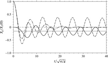
) displacements, and the straight lines indicate the corresponding large-time asymptotic values of these displacements. The dash-dot line is the vertical displacement for a cylinder in open water.

Numerical results for
 $b/a=2$
are shown in figure 4 (there is no trapped mode for this geometry and hence
 $x_{j0}=0$
in (3.66)). After a time equivalent to approximately two periods of the
 $n=0$
transient, the vertical motion settles to a slowly decaying oscillation about the mean water level, and the horizontal motion to a slowly decaying oscillation about the asymptotic value
 $X_{1}=X_{1}^{\infty }\approx -0.153X_{3}(0)$
. For the computations shown in figure 4, the Fourier integral was written in terms of the non-dimensional frequency
 $\sqrt{{\it\kappa}}$
and the range split at
 $\sqrt{{\it\kappa}}=2$
. Numerical integration was used for
 $\sqrt{{\it\kappa}}\in (0,2)$
, corresponding to the range of
 ${\it\kappa}$
displayed in figure 2, and explicit integration of the asymptotic forms given in § 3.4 was used for
 $\sqrt{{\it\kappa}}>2$
. A consequence of this is that only the first two resonances are accounted for in the calculations. However, on the scales used for the figure, only the slowly decaying oscillation arising from the lowest resonance (
 $n=0$
) is apparent; the higher-frequency oscillation due to the
 $n=1$
resonance is not discernible. From (3.11) and (3.52), the amplitude of the
 $n=1$
transient
 $$\begin{eqnarray}\displaystyle \frac{2|x_{11}|}{X_{3}(0)}\approx \frac{16(b/a-1)^{4}}{(4+{\rm\pi}^{2}){\rm\pi}^{5}}=0.004 & & \displaystyle\end{eqnarray}$$
for
 $b/a=2$
, which confirms the numerical observation that it does not contribute significantly to the motion (the amplitudes of other transients are even smaller). An indication of the accuracy of the results is obtained from the observation that the absolute errors in the initial displacements are less than
 $5\times 10^{-4}$
. For comparison, the motion of a cylinder in open water when displaced vertically a distance
 $X_{3}(0)$
and released from rest is also shown in figure 4. In this case, the sole transient is given in Maskell & Ursell (Reference Maskell and Ursell1970, equation (5.2)) and is due to resonances at
 ${\it\kappa}\approx \pm 0.8141-0.2387\text{i}$
(the approximate method in Fitzgerald & McIver (Reference Fitzgerald and McIver2009) yields
 ${\it\kappa}\approx \pm 0.82-0.29\text{i}$
). For the cylinder in the presence of a wall, the method of Fitzgerald & McIver (Reference Fitzgerald and McIver2009) gives that the lowest-frequency resonances are at
 ${\it\kappa}\approx \pm 0.96-0.01\text{i}$
, which confirms the much slower rate of decay seen in figure 4. Computation of a trapped-mode case is discussed in the following section.
4 Choice of reference point
The theory described in § 3 suggests that, for a non-zero initial vertical displacement of the cylinder, the solution to the nonlinear problem would involve a non-zero horizontal translation, and this raises questions about how to choose an appropriate linearisation of the governing equations. In the linearisation of the problem it is natural to expand all quantities about an equilibrium state in terms of a positive parameter
 ${\it\alpha}\ll 1$
that measures the disturbance from that state (John Reference John1949). This applies in particular to the position
 $\boldsymbol{X}(t)$
of the structure so that for
 $t\geqslant 0$
 $$\begin{eqnarray}\displaystyle \boldsymbol{X}(t)=\boldsymbol{X}^{(0)}+{\it\alpha}\boldsymbol{X}^{(1)}(t)+O({\it\alpha}^{2})\quad \text{as }{\it\alpha}\rightarrow 0, & & \displaystyle\end{eqnarray}$$
where
 $\boldsymbol{X}^{(0)}$
is independent of time and each
 $\boldsymbol{X}^{(m)}$
is bounded. (In general,
 $\boldsymbol{X}(t)$
is a 6-vector that locates, for example, the centre of mass of the structure and includes angles that describe its orientation.) For some components of
 $\boldsymbol{X}^{(0)}$
there is a unique equilibrium value and, for example, the vertical coordinate of the equilibrium position for a surface-piercing structure is determined by Archimedes principle and, furthermore, that equilibrium is stable. For other components, such as the horizontal coordinates, there may be no such natural choice, as a horizontal translation does not affect the presence or stability of the equilibrium for a freely floating structure. When using the linear theory to obtain an approximation for a given non-infinitesimal initial displacement (as might be required for comparison with experiment data, for example), it is perhaps natural to use the initial condition as the determining factor in the choice of the horizontal reference position, but this is not the only possible choice. The significance of the reference position
 $\boldsymbol{X}^{(0)}$
for the linear problem is that it determines the position of the structure’s surface that is used in calculations of the hydrodynamic coefficients, and different reference positions may yield different values (this is the case for the problems discussed in this paper, as the hydrodynamic coefficients for the cylinder depend upon the distance from the wall). As the hydrodynamic coefficients determine the resonances, a change in reference position may also change the resonant behaviour exhibited by the solution to the linearised problem.
Let
 $\boldsymbol{X}^{(0)}+{\it\alpha}\boldsymbol{X}^{(01)}$
be another choice of reference position so that for
 $t\geqslant 0$
the structure is at
 $$\begin{eqnarray}\displaystyle \widetilde{\boldsymbol{X}}(t)=\boldsymbol{X}^{(0)}+{\it\alpha}\boldsymbol{X}^{(01)}+{\it\alpha}\widetilde{\boldsymbol{X}}^{(1)}(t)+O({\it\alpha}^{2})\quad \text{as }{\it\alpha}\rightarrow 0. & & \displaystyle\end{eqnarray}$$
For a given
 ${\it\alpha}>0$
, the alternative linear descriptions give the same initial position of the structure provided
 $$\begin{eqnarray}\displaystyle \boldsymbol{X}^{(1)}(0)=\boldsymbol{X}^{(01)}+\widetilde{\boldsymbol{X}}^{(1)}(0). & & \displaystyle\end{eqnarray}$$
However, in general, the different reference positions mean that for
 $t>0$
 $$\begin{eqnarray}\displaystyle \boldsymbol{X}^{(1)}(t)\neq \boldsymbol{X}^{(01)}+\widetilde{\boldsymbol{X}}^{(1)}(t) & & \displaystyle\end{eqnarray}$$
because there will be differences in the calculated hydrodynamic coefficients. The choice of reference position plays no significant role in practical applications of the linearised theory provided
 $$\begin{eqnarray}\displaystyle \boldsymbol{X}^{(1)}(t)-\left[\boldsymbol{X}^{(01)}+\widetilde{\boldsymbol{X}}^{(1)}(t)\right]=O({\it\alpha})\quad \text{as }{\it\alpha}\rightarrow 0 & & \displaystyle\end{eqnarray}$$
uniformly in time. Thus, for small
 ${\it\alpha}>0$
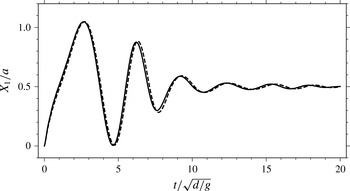
, the solutions obtained using different reference positions will differ by a small amount, regardless of the time of measurement. This is illustrated here using computations of the horizontal motion of a vertical cylinder of radius
 $a$
in water of depth
 $d$
due to the motion of a vertical wave maker (this particular example is used to illustrate the point because a rapidly decaying transient is readily obtained); see McIver (Reference McIver2012) for details of the method. Here the radius of the cylinder is chosen to be
 $a=0.1d$
and the cylinder is initially at rest at a distance
 $d$
from the wall. Calculations of the horizontal displacement
 $X_{1}(t)$
are shown in figure 5 when the motions of the cylinder and fluid are initiated by the wave-maker velocity
 $$\begin{eqnarray}\displaystyle V_{W}(t)=\mathscr{V}_{0}\cos \hat{{\it\omega}}t\,\text{e}^{-{\it\beta}t}, & & \displaystyle\end{eqnarray}$$
with
 $\hat{{\it\omega}}=2\sqrt{g/d}$
and
 ${\it\beta}=\sqrt{g/d}/2$
. The impulse arising from the start up of the wave maker gives an instantaneous jump in the velocity of the cylinder, and it is shown in McIver (Reference McIver2012) that there is an asymptotic displacement
 $X_{1}^{\infty }$
of the cylinder as
 $t\rightarrow \infty$
; here
 $\mathscr{V}_{0}$
is chosen to give
 $X_{1}^{\infty }=0.5a=0.05d$
(and hence
 $\mathscr{V}_{0}\approx 0.75a\sqrt{g/d}$
). The solution for the motion of the cylinder requires hydrodynamic coefficients whose values depend upon the distance from the wave maker of the reference position chosen for the cylinder. The results in figure 5 show calculations for two different choices of reference distance from the wall, but with the initial positions matched. In one calculation the hydrodynamic coefficients are based on the initial distance
 $d$
, but in the second calculation they are based on the final distance
 $d+X_{1}^{\infty }=1.05d$
. It can be seen that, in this case, a moderate change of reference position gives differences in the solution that are consistent with that change and that are much smaller than the initial disturbance.
The scaled horizontal displacement
 $X_{1}/a$
versus scaled time
 $t/\sqrt{d/g}$
of a cylinder of radius
 $a=0.1d$
that is initially a distance
 $d$
from a wave maker which has velocity given by (4.6). The solid and dashed lines show the solutions when the reference distances of the cylinder from the wall are
 $d$
and
 $1.05d$
, respectively.

The existence of a trapped mode provides a situation in which (4.5) may not hold for all time. Porter & Evans (Reference Porter and Evans2009) give strong numerical evidence that a freely floating half-immersed cylinder in the presence of a vertical rigid wall can support trapped modes that are free oscillations of the cylinder in a combination of sway and heave. The principal characteristics of these modes are that there is no wave radiation to infinity and, in the absence of friction, they persist for all time. Such trapped modes exist for particular values of
 $a/b$
, and one such mode occurs for
 $a/b=(a/b)_{0}\approx 0.60333$
and has a frequency that follows from
 ${\it\kappa}={\it\kappa}_{0}\approx 1.12170$
(Porter & Evans Reference Porter and Evans2009, table 1). Such a trapped mode is associated with a displacement resonance that lies on the real frequency axis so that the decay rate
 ${\it\delta}_{0}=0$
. If, in the initial-value problem of § 3, the hydrodynamic coefficients are based on a reference position equivalent to
 $a/b=(a/b)_{0}$
then a resonance occurs on the real axis at
 ${\it\kappa}={\it\kappa}_{0}$
, and the linear theory predicts that the trapped mode is excited so that the motion of the cylinder settles to an oscillation that persists for all time. In a computation made by the method of § 3.5, the horizontal component of the motion settles to an oscillation centred on
 $X_{1}^{\infty }\approx -0.182X_{3}(0)$
, and the ratio of the horizontal to vertical amplitudes of the cylinder motion is
 $0.575$
(compared with
 $0.572$
given in Porter & Evans (Reference Porter and Evans2009, table 1)). However, if, in the same initial-value problem, a different but nearby reference position is chosen, all resonances will be in the lower half of the complex plane and the motion decays as
 $t\rightarrow \infty$
. For example, calculations for
 $a/b=0.59333$
give a resonance at
 ${\it\kappa}\approx 1.1046-0.0001\text{i}$
, and for any initial displacement the motion decays to zero as
 $t\rightarrow \infty$
. Thus, for sufficiently large times, there is an order one change in the linear solution
 $\boldsymbol{X}^{(1)}(t)$
and hence, for suitable times, an order one difference from the trapped-mode case with
 $a/b=(a/b)_{0}$
as the reference position, so that (4.5) is violated.
The above comments suggest that, even with the assumption of an invisicid fluid, there may be little value in the study of the excitation of a trapped mode whose existence is sensitive to small perturbations of the geometry. Within the context of linear theory it is perhaps meaningless to attempt to distinguish between trapped modes that persist for all time, and near-trapped modes that decay with time. What happens in the nonlinear inviscid problem is an open question.
5 Time-harmonic motion excited by an incident wave
In the second main problem to be investigated, the geometry is the same as for the initial-value problem studied in § 3, but the motion of the cylinder is time-harmonic motion and is excited by an incident wave from the right with potential
 $\text{Re}\{{\it\phi}_{I}(\boldsymbol{x})\text{e}^{-\text{i}{\it\omega}t}\}$
, where
 $$\begin{eqnarray}\displaystyle {\it\phi}_{I}=\frac{-\text{i}g\mathscr{A}}{{\it\omega}}\text{e}^{-\text{i}Kx-Kz} & & \displaystyle\end{eqnarray}$$
and the positive real number
 $\mathscr{A}$
is the wave amplitude. From McIver & McIver (Reference McIver and McIver2011, equation (40)), the resulting displacements are
 $$\begin{eqnarray}\displaystyle & \displaystyle x_{1}({\it\omega})=-\frac{1}{{\it\omega}^{2}}\left\{\frac{\left[2{\it\rho}ga-{\it\omega}^{2}(M+q_{33}^{w})\right]f_{1}^{w}({\it\omega})+{\it\omega}^{2}q_{13}^{w}({\it\omega})f_{3}^{w}({\it\omega})}{2{\it\rho}ga[M+q_{11}^{w}({\it\omega})]+{\it\omega}^{2}\left\{[q_{13}^{w}({\it\omega})]^{2}-[M+q_{11}^{w}({\it\omega})][M+q_{33}^{w}({\it\omega})]\right\}}\right\} & \displaystyle \nonumber\\ \displaystyle & & \displaystyle\end{eqnarray}$$
and
 $$\begin{eqnarray}\displaystyle x_{3}({\it\omega})=\frac{-q_{13}^{w}({\it\omega})f_{1}^{w}({\it\omega})+[M+q_{11}^{w}({\it\omega})]\,f_{3}^{w}({\it\omega})}{2{\it\rho}ga[M+q_{11}^{w}({\it\omega})]+{\it\omega}^{2}\left\{[q_{13}^{w}({\it\omega})]^{2}-[M+q_{11}^{w}({\it\omega})][M+q_{33}^{w}({\it\omega})]\right\}}. & & \displaystyle\end{eqnarray}$$
The singularity in
 $x_{1}$
at
 ${\it\omega}=0$
is removable, as
 $f_{1}^{w}({\it\omega})\sim C{\it\omega}^{2}$
as
 ${\it\omega}\rightarrow 0$
, where
 $C$
is constant (McIver Reference McIver and Rahman1994, § 5). As expected, the main denominators in (5.2)–(5.3) are identical to those in (3.2)–(3.3), and hence the locations of the resonances are the same as those already determined approximately in § 3.2. Substitution of the extended wide-spacing approximations (2.12)–(2.16) into (5.2) yields
 $$\begin{eqnarray}\displaystyle \frac{x_{1}}{\mathscr{A}}=\frac{2\text{i}A_{1}}{{\rm\pi}a{\it\kappa}}\left\{\frac{\left(1-\frac{1}{4}{\rm\pi}{\it\kappa}(1+\hat{q}_{33}/M)\right)(\text{e}^{-2\text{i}{\it\kappa}b/a}-\hat{R}-\hat{T})+\text{i}{\it\kappa}\hat{A}_{3}^{2}/a^{2}}{(\text{e}^{-2\text{i}{\it\kappa}b/a}-\hat{R})G_{1}-G_{2}}\right\}, & & \displaystyle\end{eqnarray}$$
while (5.3) gives
 $$\begin{eqnarray}\displaystyle & \displaystyle \frac{x_{3}}{\mathscr{A}}=\frac{-\text{i}\hat{A}_{3}}{2a}\left\{\frac{\left(1+q_{11}/M\right)(\text{e}^{-2\text{i}{\it\kappa}b/a}-\hat{R}+\hat{T})-4\text{i}A_{1}^{2}/{\rm\pi}a^{2}}{(\text{e}^{-2\text{i}{\it\kappa}b/a}-\hat{R})G_{1}-G_{2}}\right\}; & \displaystyle\end{eqnarray}$$
here
 $G_{1}$
and
 $G_{2}$
are as defined in (3.13)–(3.14), and (2.9) has been used to write exciting forces in terms of radiated wave amplitudes.
It remains to use the wide-spacing approximations to determine approximations to the residues corresponding to the resonances (as before, the
 $n=0$
resonance is not accessible by the method used here). In these time-harmonic calculations it is perhaps more natural to determine the residues when the displacements are regarded as functions of
 ${\it\kappa}$
, and this is done here. First of all, for
 $j\in \{1,3\}$
write
 $x_{j}/\mathscr{A}=f_{j}({\it\kappa})/h({\it\kappa})$
, where
 $h$
is defined in (3.47) so that, in particular,
 $h(\widetilde{{\it\kappa}})=0$
for a resonance at
 ${\it\kappa}=\widetilde{{\it\kappa}}$
. It then follows from (5.4) that, after drawing on the asymptotic results given in §§ 3.2 and 3.3 and in appendix B,
 $$\begin{eqnarray}\displaystyle f_{1}(\widetilde{{\it\kappa}}) & = & \displaystyle \frac{2\text{i}A_{1}}{{\rm\pi}a\widetilde{{\it\kappa}}G_{1}}\left\{\left(1-\frac{1}{4}{\rm\pi}\widetilde{{\it\kappa}}(1+\hat{q}_{33}/M)\right)(G_{2}/G_{1}-\hat{T})+\text{i}\widetilde{{\it\kappa}}\hat{A}_{3}^{2}/a^{2}\right\}\nonumber\\ \displaystyle & {\sim} & \displaystyle -\frac{32\text{i}{\rm\pi}^{2}\text{e}^{-3\text{i}\widetilde{{\it\kappa}}}}{(4+{\rm\pi}^{2})^{2}\widetilde{{\it\kappa}}^{4}}\quad \text{as }\widetilde{{\it\kappa}}\rightarrow \infty .\end{eqnarray}$$
Similar arguments to those in § 3.3 then give the residue
 $$\begin{eqnarray}\displaystyle \frac{x_{1n}^{({\it\kappa})}}{\mathscr{A}}\sim \frac{16{\rm\pi}^{2}\text{e}^{-\text{i}{\it\kappa}_{n}}}{(4+{\rm\pi}^{2})^{2}(b/a-1){\it\kappa}_{n}^{4}}\sim \frac{16(b/a-1)^{3}\,\text{e}^{-\text{i}{\it\kappa}_{n}}}{(4+{\rm\pi}^{2})^{2}{\rm\pi}^{2}n^{4}}\quad \text{as }n\rightarrow \infty . & & \displaystyle\end{eqnarray}$$
Similarly
 $$\begin{eqnarray}\displaystyle & \displaystyle f_{3}(\widetilde{{\it\kappa}})=\frac{-\text{i}\hat{A}_{3}}{2aG_{1}}\left\{\left(1+q_{11}/M\right)(G_{2}/G_{1}+\hat{T})-4\text{i}A_{1}^{2}/{\rm\pi}a^{2}\right\}\sim \frac{32\text{i}\,\text{e}^{-3\text{i}\widetilde{{\it\kappa}}}}{(4+{\rm\pi}^{2})\widetilde{{\it\kappa}}^{5}}\quad \text{as }\widetilde{{\it\kappa}}\rightarrow \infty & \displaystyle \nonumber\\ \displaystyle & & \displaystyle\end{eqnarray}$$
and hence
 $$\begin{eqnarray}\displaystyle \frac{x_{3n}^{({\it\kappa})}}{\mathscr{A}}\sim -\frac{16\,\text{e}^{-\text{i}{\it\kappa}_{n}}}{(4+{\rm\pi}^{2})(b/a-1){\it\kappa}_{n}^{5}}\sim -\frac{16(b/a-1)^{4}\,\text{e}^{-\text{i}{\it\kappa}_{n}}}{(4+{\rm\pi}^{2}){\rm\pi}^{5}n^{5}}\quad \text{as }n\rightarrow \infty . & & \displaystyle\end{eqnarray}$$
As noted immediately before (3.55), as
 ${\it\kappa}$
varies near a resonance the maximum modulus of the contribution to the displacement from that resonance is
 $|x_{jn}^{({\it\kappa})}|/|{\it\tau}_{n}|$
. From the above results and (3.38), as
 $n\rightarrow \infty$
 $$\begin{eqnarray}\displaystyle \frac{|x_{jn}^{({\it\kappa})}|}{|{\it\tau}_{n}|}\sim \left\{\begin{array}{@{}ll@{}}\displaystyle \mathscr{A},\quad & j=1;\\ \displaystyle \frac{(4+{\rm\pi}^{2})(b/a-1)\mathscr{A}}{{\rm\pi}^{3}n},\quad & j=3.\end{array}\right. & & \displaystyle\end{eqnarray}$$
As for the initial-value problem described in § 3, a given resonance is most prominently displayed in the sway displacement but, in this case, there is no decay with increasing
 $n$
. Thus, an incident wave with
 ${\it\kappa}\approx {\it\kappa}_{n}$
will always excite a significant response in sway, regardless of the value of
 $n$
, but the heave response decays to zero as
 $n\rightarrow \infty$
.
Away from resonance, (5.4) and (5.5) give, respectively,
 $$\begin{eqnarray}\displaystyle \frac{x_{1}}{\mathscr{A}}\sim \frac{4{\rm\pi}\,\text{e}^{-\text{i}{\it\kappa}}}{(4+{\rm\pi}^{2}){\it\kappa}^{2}}\quad \text{and}\quad \frac{x_{3}}{\mathscr{A}}\sim \frac{4\,\text{e}^{-\text{i}{\it\kappa}}}{{\rm\pi}{\it\kappa}^{3}}\quad \text{as }{\it\kappa}\rightarrow \infty . & & \displaystyle\end{eqnarray}$$
Unlike the initial-value problem of § 3, these ‘background’ decay rates are both faster than those given in (5.10) for the resonances, and hence the resonances remain relatively prominent as
 $n$
increases.
The modulus of the scaled displacements
 $|x_{j}|/\mathscr{A}$
versus
 ${\it\kappa}$
for a half-immersed cylinder of radius
 $a$
at a distance
 $2a$
from a rigid vertical wall subject to a time-harmonic incident wave of amplitude
 $\mathscr{A}$
. The solid and dashed lines show, respectively, the sway (
 $j=1$
) and heave (
 $j=3$
) displacements, and the inset shows the resonance near
 ${\it\kappa}=6.35$
in more detail.

Numerical results for the magnitudes of the displacements are shown in figure 6 (the results were computed using an extension of the multipole method given in Porter (Reference Porter2008)). The most prominent resonance is that just below
 ${\it\kappa}=1$
, which is a perturbation of that found for the cylinder when in open water. The standing-wave resonances are much less significant, and the behaviours confirm those predicted by the asymptotic results in (5.10), with, in particular, the peak sway displacements being close to the wave amplitude. The accuracy of the approximations is confirmed for the resonance shown in the inset to the figure, with, in particular, the peak heave displacement being close to the predicted value of approximately
 $0.2\mathscr{A}$
. Like the initial-value problem discussed in § 3, for this geometry the asymptotic theory, which is formally valid as the resonance index
 $n\rightarrow \infty$
, predicts with good accuracy the behaviour at resonance for small
 $n$
.
6 Discussion
In this paper an approximate technique, based on high-frequency asymptotics, is used to obtain information about the complex resonances associated with near-standing waves between a floating cylinder and a vertical wall. The technique is applied to the standard hydrodynamic coefficients, and also to the displacements in two particular problems for a freely floating cylinder: the time-dependent motion that follows the release from rest of a cylinder displaced vertically, and the time-harmonic motion that is forced by an incident plane wave. In these two problems the resonances in the displacements are at the same locations, but the residues at the resonance poles differ. Among the results obtained is an approximation to the shift in frequency of the displacement resonance relative to that of the hydrodynamic coefficients, and a demonstration that the displacement resonances are further from the real frequency axis.
The method used here to describe complex resonances employs a wide-spacing approximation. The standard such approximation would use only plane-wave interactions between the cylinder and the wall, but here an extended approximation that accounts for the leading-order effects of the evanescent modes is employed. As far as the location of complex resonances is concerned, and to the orders obtained in the high-frequency asymptotics, it is found that only the imaginary parts of the resonances for the hydrodynamic coefficients are affected by inclusion of evanescent effects, while the displacement resonances are unaffected.
A number of results follow from the approximations to the residues. For example, in the initial-value problem the amplitude of the vertical transient associated with a particular resonance is smaller than that of the corresponding horizontal transient, while in the time-harmonic problem the amplitudes of sway resonances do not decay with increasing frequency. In addition, it is pointed out that different choices for the equilibrium state – obtained, for example, by small horizontal translations – can lead to solutions that differ sufficiently for the assumptions of the linearised theory to be violated at large times.
The motion of a cylinder placed in open water displays a single resonance due to the hydrostatic spring. Hence, for the problems discussed in detail here, it is natural to consider what happens to each standing-wave resonance as the non-dimensional distance
 $b/a$
of the cylinder from the wall increases. It should be noted that the standing-wave resonances exist for any finite
 $b/a$
, and that a plane propagating wave generated at the cylinder does not decay as it travels between the cylinder and wall. For a fixed index
 $n$
, equations (3.37) and (3.38) show that an increase in
 $b/a$
moves the resonance to a lower frequency and rapidly away from the real axis. A move to lower frequencies within the high-frequency regime means that, in the frequency domain, cylinder motions generate waves of larger amplitude so that interactions with the wall may be stronger. In the initial-value problem, equations (3.52) and (3.54) reveal an increase in the amplitudes of the transients with increasing
 $b/a$
, although this is offset by the faster decay rate due to the movement of the resonance away from the real axis. In the time-harmonic problem, equation (5.10) shows that an increase in
 $b/a$
has no leading-order effect on the contribution of the resonance to sway displacement, while the magnitude of the heave resonance increases. All of the explicit results obtained here are based on the assumption that a resonance is close to the real axis so that a full analysis of the effect of increasing the distance from the wall requires calculations for complex frequency such as used, for example, in Meylan & Tomic (Reference Meylan and Tomic2012, § 3).
A related geometry, that could be studied by the methods described here, is that of two identical half-immersed cylinders that are rigidly connected so that they move together. If such a structure in open water is displaced vertically and released from rest then there is no horizontal motion, and hence the expressions for the frequency-domain displacements do not contain any terms relating to sway. As a consequence, the relations that determine the locations of the resonances differ from those used in this paper, and hence the locations themselves will differ from those found here.
Newman (Reference Newman1977) used strip theory to calculate the motions of a floating torus for which the radius of the circular cross-section is much less that the radius of the toroidal ring. The procedure requires knowledge of the hydrodynamic properties of the cross-sectional geometry, which is just the two-dimensional half-immersed circle considered here. Thus, the procedures used in the present work could be applied to a slender torus, with the only significant change being a suitable adaptation of the wide-spacing approximation to the toroidal geometry.
Appendix A. The extended wide-spacing approximation
Given below are outline derivations of the expressions given in § 2.2 and obtained from the extended wide-spacing approximation McIver (Reference McIver2014).
In the radiation problems the heave force coefficient is obtained directly from McIver (Reference McIver2014), so it is sufficient to consider the forced motion of the cylinder in sway. The wall may be replaced by an image cylinder with axis at
 $x=-2b$
that is moving in antiphase with the original cylinder. To make direct comparison with the results in McIver (Reference McIver2014), the image is identified as cylinder 1 and the original as cylinder 2, while the intersections of these cylinders with the undisturbed free surface are denoted by
 $A$
,
 $B$
,
 $C$
and
 $D$
in order of increasing
 $x$
(McIver Reference McIver2014, figure 1). In McIver (Reference McIver2014),
 $I_{P}$
and
 $J_{P}$
are used to denote, respectively, the amplitudes of the waves propagating towards and away from
 $P\in \{A,B,C,D\}$
. The amplitudes
 $J_{P}$
are scaled by
 $K$
and are determined from applications of McIver (Reference McIver2014, equation (6.11)) so that, in particular,
 $$\begin{eqnarray}\displaystyle J_{B}=-KA_{1}+J_{C}\,\text{e}^{2\text{i}{\it\kappa}b/a}R+J_{B}\,\text{e}^{2\text{i}{\it\kappa}b/a}{\it\epsilon}^{2}p_{3} & & \displaystyle\end{eqnarray}$$
(
 $p_{3}$
is defined after (2.11) of this paper). On the right-hand side of (A 1), the first term represents the wave radiated towards the right by cylinder 1 when in isolation, the second term arises from the reflection of the wave propagating to the left from cylinder 2, and the third term arises from the evanescent terms generated when the wave propagating to the right between the cylinders interacts with cylinder 1. From the symmetry of the problem
 $J_{B}=J_{C}$
and hence
 $$\begin{eqnarray}\displaystyle J_{C}=\frac{-KA_{1}\,\text{e}^{-2\text{i}{\it\kappa}b/a}}{\text{e}^{-2\text{i}{\it\kappa}b/a}-\hat{R}}, & & \displaystyle\end{eqnarray}$$
where
 $\hat{R}$
is defined in (2.10). From McIver (Reference McIver2014, equations (2.11) and (6.14))
 $$\begin{eqnarray}\displaystyle q_{1p}^{w}=\hat{q}_{1p}+\frac{J_{C}\,\text{e}^{2\text{i}{\it\kappa}b/a}}{\text{i}{\it\omega}K}\left[\text{}^{B}X_{2p}+\text{}^{C}X_{2p}\right], & & \displaystyle\end{eqnarray}$$
where each
 $\text{}^{P}X_{2p}$
is a force arising in a certain subsidiary scattering problem (McIver Reference McIver2014, § 4). From McIver (Reference McIver2014, equations (4.24) and (4.25))
 $$\begin{eqnarray}\displaystyle \text{}^{B}X_{21}=0\quad \text{and}\quad \text{}^{C}X_{21}=-{\it\omega}{\it\rho}A_{1}=-\frac{\text{i}{\it\omega}f_{1}}{g\mathscr{A}} & & \displaystyle\end{eqnarray}$$
so that
 $$\begin{eqnarray}\displaystyle q_{11}^{w}=q_{11}-\frac{\text{i}{\it\rho}A_{1}^{2}}{\text{e}^{-2\text{i}{\it\kappa}b/a}-\hat{R}}, & & \displaystyle\end{eqnarray}$$
while
 $$\begin{eqnarray}\displaystyle \text{}^{B}X_{23}={\it\omega}{\it\rho}{\it\epsilon}^{2}{\it\kappa}{\it\sigma}A_{3}=\frac{\text{i}{\it\omega}{\it\epsilon}^{2}{\it\kappa}{\it\sigma}f_{3}}{g\mathscr{A}}\quad \text{and}\quad \text{}^{C}X_{23}={\it\omega}{\it\rho}A_{3}=\frac{\text{i}{\it\omega}f_{3}}{g\mathscr{A}} & & \displaystyle\end{eqnarray}$$
so that
 $$\begin{eqnarray}\displaystyle q_{13}^{w}=\frac{\text{i}{\it\rho}A_{1}\hat{A}_{3}}{\text{e}^{-2\text{i}{\it\kappa}b/a}-\hat{R}}. & & \displaystyle\end{eqnarray}$$
In the scattering problem the wall boundary condition is enforced by taking plane waves of equal amplitude to be incident from both left and right. Thus, in McIver (Reference McIver2014, equations (5.1)), the incoming wave amplitudes are chosen as
 $I_{A}=I_{B}=1$
, and then the amplitude
 $J_{B}=I_{C}\,\text{e}^{-2\text{i}{\it\kappa}b/a}$
of the plane wave propagating away from
 $B$
is
 $$\begin{eqnarray}\displaystyle J_{B}=T+I_{B}R+I_{C}{\it\epsilon}^{2}p_{3}+{\it\epsilon}^{2}p_{3}. & & \displaystyle\end{eqnarray}$$
On the right-hand side of (A 8), the first term arises from the transmission past cylinder 1 of the incident wave from the left, the second term arises from the reflection at cylinder 1 of the wave travelling towards
 $B$
, the third term arises from the evanescent terms generated when the wave propagating to the right interacts with cylinder 1, and the fourth term arises from the evanescent terms generated when the incident wave from the right interacts with cylinder 1. From the symmetry of the problem
 $I_{B}=I_{C}$
, and hence
 $$\begin{eqnarray}\displaystyle I_{C}=\frac{\hat{T}}{\text{e}^{-2\text{i}{\it\kappa}b/a}-\hat{R}}, & & \displaystyle\end{eqnarray}$$
where
 $\hat{T}$
is defined in (2.10). From McIver (Reference McIver2014, equation (5.20))
 $$\begin{eqnarray}\displaystyle f_{p}^{w}=\frac{g\mathscr{A}}{\text{i}{\it\omega}}\left[\text{}^{A}X_{2p}+I_{C}\left(\text{}^{B}X_{2p}+\text{}^{C}X_{2p}\right)+\text{}^{D}X_{2p}\right] & & \displaystyle\end{eqnarray}$$
and, in addition to the above values for
 $\text{}^{C}X_{2p}$
,
 $$\begin{eqnarray}\displaystyle \text{}^{A}X_{21}=0,\quad \text{}^{A}X_{23}=\text{}^{B}X_{23},\quad \text{}^{D}X_{21}=-\text{}^{C}X_{21},\quad \text{}^{D}X_{23}=\text{}^{C}X_{23} & & \displaystyle\end{eqnarray}$$
so that
 $$\begin{eqnarray}\displaystyle f_{1}^{w}=f_{1}\left[1-\frac{\hat{T}}{\text{e}^{-2\text{i}{\it\kappa}b/a}-\hat{R}}\right] & & \displaystyle\end{eqnarray}$$
and
 $$\begin{eqnarray}\displaystyle f_{3}^{w}=\hat{f}_{3}\left[1+\frac{\hat{T}}{\text{e}^{-2\text{i}{\it\kappa}b/a}-\hat{R}}\right]. & & \displaystyle\end{eqnarray}$$
Appendix B. High-frequency expansions
Here the high-frequency expansion of
 ${\it\epsilon}^{2}p_{3}/R$
is developed, and further information is obtained about the expansions of other quantities. First of all, further terms are introduced into the expansions of
 $R$
and
 $A_{3}$
so that as
 ${\it\kappa}\rightarrow \infty$
 $$\begin{eqnarray}\displaystyle R\sim \text{e}^{-2\text{i}{\it\kappa}}\left[1-\frac{\text{i}}{2{\it\kappa}}+\frac{1}{{\it\kappa}^{2}}\left(-\frac{1}{8}+\frac{2\text{i}}{3{\rm\pi}}\right)+\frac{1}{{\it\kappa}^{3}}\left(\frac{1}{3{\rm\pi}}+\text{i}\,R_{32}\right)+\frac{1}{{\it\kappa}^{4}}\left(R_{41}+\text{i}\,R_{42}\right)\right] & & \displaystyle\end{eqnarray}$$
and
 $$\begin{eqnarray}\displaystyle A_{3} & {\sim} & \displaystyle -\frac{4\text{i}a\,\text{e}^{-\text{i}{\it\kappa}}}{{\it\kappa}^{2}}\left[1+\frac{2}{{\rm\pi}{\it\kappa}}\left({\it\gamma}+\log 2{\it\kappa}-3-\frac{\text{i}{\rm\pi}}{8}\right)+\frac{1}{{\it\kappa}^{2}}\left(A_{3,21}+\text{i}\,A_{3,22}\right)\right.\nonumber\\ \displaystyle & & \displaystyle +\left.\frac{1}{{\it\kappa}^{3}}\left(A_{3,31}+\text{i}\,A_{3,32}\right)+\frac{1}{{\it\kappa}^{4}}\left(A_{3,41}+\text{i}\,A_{3,42}\right)\right],\end{eqnarray}$$
where each
 $R_{mn}$
and
 $A_{l,mn}$
is real and may contain terms in
 $\log {\it\kappa}$
and its non-negative powers. Substitution of these, together with the expansion of
 $T$
in (3.18), into the identity
 $R+T=-A_{3}/\overline{A}_{3}$
(Linton & McIver Reference Linton and McIver2001, equation (1.74)) and equating like terms in
 ${\it\kappa}$
yields, in particular,
 $$\begin{eqnarray}\displaystyle & \displaystyle A_{3,22}=\frac{-3{\it\gamma}-3\log 2{\it\kappa}+11}{6{\rm\pi}}, & \displaystyle\end{eqnarray}$$
 $$\begin{eqnarray}\displaystyle & \displaystyle A_{3,32}=\frac{-48{\rm\pi}^{2}A_{3,21}+128{\it\gamma}+128\log 2{\it\kappa}+96{\rm\pi}^{2}R_{32}-3{\rm\pi}^{2}-384}{192{\rm\pi}^{2}}, & \displaystyle\end{eqnarray}$$
and
 $$\begin{eqnarray}\displaystyle & A_{3,42}=\displaystyle \frac{32A_{3,21}-3(8{\rm\pi}A_{3,31}+{\it\gamma}-32({\it\gamma}-3)R_{32}-16{\rm\pi}R_{42}-37)+(96R_{32}-3)\log 2{\it\kappa}}{96{\rm\pi}} & \displaystyle \nonumber\\ \displaystyle & & \displaystyle\end{eqnarray}$$
(these, and similar calculations, were carried out with the aid of a computer algebra system). These results on the asymptotics of
 $A_{3}$
are then sufficient to give
 $$\begin{eqnarray}\displaystyle \displaystyle \frac{{\it\epsilon}^{2}p_{3}}{R} & = & \displaystyle -\frac{\text{i}A_{3}^{2}}{4{\rm\pi}b^{2}R}=\frac{a^{2}}{b^{2}}\left[\frac{4\text{i}}{{\rm\pi}{\it\kappa}^{4}}+\frac{16\text{i}({\it\gamma}+\log 2{\it\kappa}-3)}{{\rm\pi}^{2}{\it\kappa}^{5}}\right.\nonumber\\ \displaystyle & & \displaystyle \displaystyle +\,\frac{\text{i}\left({\rm\pi}^{2}(32A_{3,21}+1)+128({\it\gamma}-3)\log 2{\it\kappa}+64({\it\gamma}-3)^{2}+64[\log 2{\it\kappa}]^{2}\right)}{4{\rm\pi}^{3}{\it\kappa}^{6}}\nonumber\\ \displaystyle & & \displaystyle \displaystyle +\,\frac{\text{i}(48A_{3,21}({\it\gamma}-3)+(48A_{3,21}+3)\log 2{\it\kappa}+24{\rm\pi}A_{3,31}+3{\it\gamma}-11)}{3{\rm\pi}^{2}{\it\kappa}^{7}}\nonumber\\ \displaystyle & & \displaystyle \displaystyle \times \left.\frac{1}{{\it\kappa}^{8}}\left(-\frac{8}{{\rm\pi}^{2}}+\text{i}p_{3,82}\right)\right]\quad \text{as }{\it\kappa}\rightarrow \infty ,\end{eqnarray}$$
where
 $p_{3,82}\in \mathbb{R}$
and contains terms in
 $\log {\it\kappa}$
and
 $[\log {\it\kappa}]^{2}$
. The significant features of this expansion are that the first real term is in the coefficient of
 $1/{\it\kappa}^{8}$
, and that it is known explicitly.
With
 $$\begin{eqnarray}\displaystyle & \displaystyle A_{1}\sim -\frac{2\text{i}a\,\text{e}^{-\text{i}{\it\kappa}}}{{\it\kappa}}\biggl[1+\frac{2}{{\rm\pi}{\it\kappa}}\left({\it\gamma}+\log 2{\it\kappa}-2-\frac{\text{i}{\rm\pi}}{8}\right)+\frac{1}{{\it\kappa}^{2}}\left(A_{1,21}+\text{i}\,A_{1,22}\right)\biggr] & \displaystyle\end{eqnarray}$$
the identity
 $R-T=-A_{1}/\overline{A}_{1}$
(Linton & McIver Reference Linton and McIver2001, equation (1.74)) yields
 $$\begin{eqnarray}\displaystyle A_{1,22}=\frac{-3{\it\gamma}-3\log 2{\it\kappa}+8}{6{\rm\pi}} & & \displaystyle\end{eqnarray}$$
and then
 $$\begin{eqnarray}\displaystyle S & = & \displaystyle \frac{G_{2}}{G_{1}\hat{R}}=-\frac{8\text{i}{\rm\pi}}{\left(4+{\rm\pi}^{2}\right){\it\kappa}^{2}}+\frac{8\text{i}\left({\rm\pi}^{3}{\it\mu}_{11,1}+4\left(4+{\rm\pi}^{2}\right)(2-{\it\gamma}-\log 2{\it\kappa})\right)}{\left(4+{\rm\pi}^{2}\right)^{2}{\it\kappa}^{3}}\nonumber\\ \displaystyle & & \displaystyle +\,\frac{1}{{\it\kappa}^{4}}\left(-\frac{64{\rm\pi}^{2}}{\left(4+{\rm\pi}^{2}\right)^{2}}+\text{i}S_{42}\right),\end{eqnarray}$$
where
 ${\it\mu}_{11,1}=-0.73789$
(see (3.21)) and
 $S_{42}\in \mathbb{R}$
contains terms in
 $\log {\it\kappa}$
and
 $[\log {\it\kappa}]^{2}$
as well some unknown coefficients in the expansions of the hydrodynamic coefficients. The leading-order effects of the evanescent terms (as a function of
 ${\it\kappa}$
) also contribute to
 $S_{42}$
.