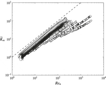
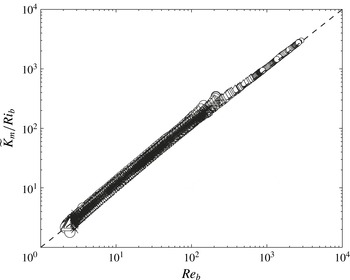
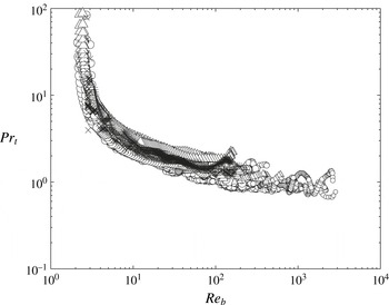
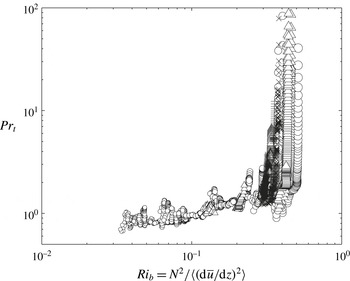
1. Introduction
The idea of a turbulent diapycnal diffusivity,
 $K_{{\it\rho}}$
, is often introduced to represent the irreversible flux of mass across isopycnal surfaces in a density-stratified fluid which experiences irreversible turbulent mixing. It may be defined most generally as the ratio of a scalar flux to its vertical gradient as:
 $$\begin{eqnarray}K_{{\it\rho}}=-\frac{\text{flux}}{\text{gradient}}.\end{eqnarray}$$
As noted by Winters & D’Asaro (Reference Winters and D’Asaro1996) and Barry et al. (Reference Barry, Ivey, Winters and Imberger2001), the fundamental difference between models of
 $K_{{\it\rho}}$
arises due to the different definitions adopted for both the scalar flux and its associated gradient in (1.1). At present, the representations proposed by Osborn & Cox (Reference Osborn and Cox1972) and Osborn (Reference Osborn1980) are still widely employed in the parameterization of small-scale diapycnal mixing in large-scale numerical models of the ocean general circulation (e.g. Danabasoglu et al.
Reference Danabasoglu, Bates, Briegleb, Jayne, Jochum, Large, Peacock and Yeager2012) and also to infer
 $K_{{\it\rho}}$
from oceanographic experimental measurements (e.g. Waterhouse et al.
Reference Waterhouse, MacKinnon, Nash, Alford, Kunze, Simmons, Polzin, St. Laurent, Sun, Pinkel, Talley, Whalen, Huussen, Carter, Fer, Waterman, Naveira Garabato, Sanford and Lee2014). Given the approximate nature of these models (Davis Reference Davis1994; Mashayek & Peltier Reference Mashayek and Peltier2013) and the fact that they do not distinguish between reversible ‘stirring’ and irreversible ‘mixing’ (as discussed in Winters et al.
Reference Winters, Lombard, Riley and D’Asaro1995 and Caulfield & Peltier Reference Caulfield and Peltier2000), an accurate definition for
 $K_{{\it\rho}}$
using an isoscalar coordinate system was proposed by Winters & D’Asaro (Reference Winters and D’Asaro1996) (hereinafter referred to as WD96). One goal of the present work is to analytically recast their definition of
 $K_{{\it\rho}}$
into a more familiar ‘Osborn-like’ expression and to clarify its dependence on an accurately defined irreversible mixing efficiency,
 $\mathscr{E}$
, and buoyancy Reynolds number
 $\mathit{Re}_{b}$
.
Mixing efficiency,
 $\mathscr{E}$
, may be defined as the ‘useful’ expenditure of total mechanical energy that is invested in irreversible mixing (Caulfield & Peltier Reference Caulfield and Peltier2000), which for a Boussinesq flow leads to a monotonic increase of a background potential energy (BPE) of the system (Winters et al.
Reference Winters, Lombard, Riley and D’Asaro1995; Tailleux Reference Tailleux2009) that is to be distinguished from the available potential energy that can be converted into kinetic energy (Lorenz Reference Lorenz1955). It has become common practice to assume a canonical value of 0.2 for an assumed constant value of mixing efficiency, through which the diapycnal diffusivity is estimated based on the approximate formulation of Osborn (Reference Osborn1980). However, there is continuing debate on the relevance of this value to the full range of accessible turbulent regimes in geophysical flows (Ivey, Winters & Koseff Reference Ivey, Winters and Koseff2008). This issue has therefore prompted the development of alternative expressions for scalar diffusivity based on a variety of length scale arguments (e.g. see Ivey & Imberger Reference Ivey and Imberger1991; Barry et al.
Reference Barry, Ivey, Winters and Imberger2001; Shih et al.
Reference Shih, Koseff, Ivey and Ferziger2005) that may be employed to interpret the measurements of turbulence related processes in environmental flows (Dunckley et al.
Reference Dunckley, Koseff, Steinbuck, Monismith and Genin2012; Bluteau, Jones & Ivey Reference Bluteau, Jones and Ivey2013; Bouffard & Boegman Reference Bouffard and Boegman2013). The modest reformulation of
 $K_{{\it\rho}}$
, to be presented in what follows, is a direct mathematical consequence of the governing Boussinesq equations and will lead us to advocate the use of an ‘Osborn-like’ formula with no limiting approximations, provided that a correct definition of
 $\mathscr{E}$
is employed. Moreover, this reformulation will be shown to reinforce the importance of the previously presented length scale arguments suggesting that
 $K_{{\it\rho}}$
should depend strongly upon
 $\mathit{Re}_{b}$
.
The buoyancy Reynolds number,
 $\mathit{Re}_{b}$
(or as it is also sometimes referred to, the turbulence intensity parameter), measures the extent of the inertial subrange that is characterized by the ratio of the Ozmidov to the Kolmogorov length scales (to the power
 $4/3$
) (e.g. see Smyth & Moum Reference Smyth and Moum2000b
). This dimensionless parameter has been suggested to be one of the two dynamically relevant parameters required for the characterization of stratified turbulence (e.g. see Brethouwer et al.
Reference Brethouwer, Billant, Lindborg and Chomaz2007 and Ivey et al.
Reference Ivey, Winters and Koseff2008). The second parameter required for such characterization may be thought to be the gradient Richardson number
 $\mathit{Ri}_{b}$
(Linden Reference Linden1979; Fernando Reference Fernando1991) which characterizes the relative strengths of density stratification and velocity shear. These two parameters are respectively defined as:
 $$\begin{eqnarray}\mathit{Re}_{b}=\frac{{\it\varepsilon}_{k}}{{\it\nu}N^{2}},\quad \mathit{Ri}_{b}=\frac{N^{2}}{S^{2}},\end{eqnarray}$$
where
 ${\it\varepsilon}_{k}$
is the viscous dissipation of kinetic energy (to be precisely defined in what follows),
 ${\it\nu}$
is kinematic viscosity,
 $N$
is the Brunt–Väisälä frequency and
 $S$
is the vertical shear. Here we employ a bulk measure of the gradient Richardson number in which
 $N^{2}$
and
 $S^{2}$
are individually vertically averaged over the same appropriate length scale.
In addition to
 $K_{{\it\rho}}$
, the momentum diffusivity (or eddy viscosity),
 $K_{m}$
, is also required to characterize the subgrid-scale diffusion of momentum and it too must therefore be parameterized in large-scale numerical models of geophysical flows (Klymak, Legg & Pinkel Reference Klymak, Legg and Pinkel2010; Danabasoglu et al.
Reference Danabasoglu, Bates, Briegleb, Jayne, Jochum, Large, Peacock and Yeager2012). A key parameter which measures the relative importance of these two turbulent diffusivities is the turbulent Prandtl number
 $\mathit{Pr}_{t}=K_{m}/K_{{\it\rho}}$
. Venayagamoorthy & Stretch (Reference Venayagamoorthy and Stretch2010) have recently studied the variations of
 $\mathit{Pr}_{t}$
in the special case of homogeneous sheared and stratified turbulence in which they distinguished reversible from irreversible contributions to
 $K_{m}$
by drawing an analogy to a formulation in the stationary turbulence limit (based on simplified energy and scalar balance equations) and proposing a new formulation for
 $K_{m}$
for non-stationary homogeneous stratified and sheared turbulent flows. A second primary goal in this paper is to propose an expression for
 $\mathit{Pr}_{t}$
applicable to any stratified Boussinesq flow at sufficiently high
 $\mathit{Re}$
.
Any useful parameterization of
 $K_{{\it\rho}}$
and
 $K_{m}$
(or
 $\mathit{Pr}_{t}$
) should rely on a study which not only isolates the signature of irreversible mixing on turbulent diffusivity, but also properly identifies the aforementioned parametric dependences. In this regard, direct numerical simulation (DNS) provides the ideal tool to analyse stratified turbulent mixing events. Nonetheless, previous DNS efforts (e.g. Smyth, Moum & Caldwell Reference Smyth, Moum and Caldwell2001; Shih et al.
Reference Shih, Koseff, Ivey and Ferziger2005; Smyth, Nash & Moum Reference Smyth, Nash and Moum2005; Mashayek & Peltier Reference Mashayek and Peltier2013) have not consistently employed adequately precise definitions of these important quantities, namely
 $\mathscr{E}$
,
 $K_{{\it\rho}}$
and
 $K_{m}$
(or
 $\mathit{Pr}_{t}$
). Here, by use of the phrase ‘adequately precise’ we mean definitions that fully distinguish between the reversible and irreversible contributions to the scalar and momentum flux related processes. Furthermore, aside from the study by Shih et al. (Reference Shih, Koseff, Ivey and Ferziger2005) (hereinafter referred to as SKIF), who focused on the special case of homogeneous sheared and stratified turbulence, to the best of our knowledge there has been no other DNS study aimed at characterizing the dependence of
 $\mathscr{E}$
,
 $K_{{\it\rho}}$
and
 $K_{m}$
on the dynamically relevant parameters of stratified turbulence (e.g.
 $\mathit{Re}_{b}$
and
 $\mathit{Ri}_{b}$
). In this paper, our intention is to begin to address both these aspects of the stratified turbulence problem through the analysis of an extensive series of three-dimensional DNS dataset of the much more geophysically relevant case of inhomogeneously stratified and sheared turbulence that is generated after a laminar two-dimensional Kelvin–Helmholtz (KH) wave ‘breaks’ at high initial Reynolds numbers (to be denoted henceforth as the KH ansatz). Nonetheless, we foresee a significant need for further numerical and experimental effort focusing on stratified turbulence with a wider range of turbulent generation mechanisms in order to fully establish the parametric dependences of these critical characteristics of stratified turbulence.
The remainder of this paper consists of two distinct parts. In the first part in §§ 2 and 3, we first review the available models that continue to be employed in the estimation of
 $K_{{\it\rho}}$
and
 $K_{m}$
, following which we propose improved expressions for the diapycnal diffusivity
 $K_{{\it\rho}}$
and eddy viscosity
 $K_{m}$
(and hence
 $\mathit{Pr}_{t}$
) in stratified Boussinesq turbulence. Arguments presented in § 2.3 essentially transform the problem of parameterizing diapycnal diffusivity into the problem of correctly determining irreversible mixing efficiency. The second part of this paper, in § 4, describes our numerical methodology and provides the results of an extensive series of DNS analyses of turbulence characteristics based on the KH ansatz. While the first part of the paper relies solely upon the structure of the underlying Boussinesq equations (and is therefore independent of flow configuration), the second part is specific to our choice of model problem. Concluding remarks that follow from the analyses we have performed are offered in § 5.
2. Scalar diffusivity and mixing efficiency
Our primary goal is to moderately build upon and to extend the previous work of WD96 in order to derive a revised expression for diapycnal diffusivity. This reformulation will lead to an expression of Osborn (Reference Osborn1980) form, but one that eliminates all the assumptions on which it was originally based, which should therefore constitute a useful basis for improved parameterizations of diapycnal diffusivity. In all that follows we will be providing non-dimensional representations for various models of
 $K_{{\it\rho}}$
by normalizing them by the molecular diffusivity,
 ${\it\kappa}$
, i.e.
 $\widetilde{K}_{{\it\rho}}=K_{{\it\rho}}/{\it\kappa}$
. This non-dimensionalization will prove useful for the purpose of comparing
 $K_{{\it\rho}}$
for fluids characterized by different molecular Prandtl numbers. Because the turbulent diffusivity is inevitably several orders of magnitude greater than its molecular counterpart, this non-dimensional diffusivity would be expected to reach high values of
 $O(10^{1}{-}10^{4})$
, regardless of the calculation methodology.
2.1. Existing models of scalar diffusivity
We begin by reviewing four different methods of calculating
 $K_{{\it\rho}}$
, some of which are most commonly employed in numerical and experimental studies. These methods include: (i) the Prandtl mixing length model denoted by
 $K_{{\it\rho}}^{ml}$
, (ii) the Osborn formula,
 $K_{{\it\rho}}^{osb}$
, (iii) the Osborn–Cox formula
 $K_{{\it\rho}}^{cox}$
and finally (iv) the Winters–D’Asaro formula,
 $K_{{\it\rho}}^{\ast }$
.
The Prandtl mixing length model is sometimes referred to as the ‘direct’ method of calculating
 $K_{{\it\rho}}$
(Ivey et al.
Reference Ivey, Winters and Koseff2008; Bouffard & Boegman Reference Bouffard and Boegman2013). In fact, the historical difficulties associated with measuring and interpreting the turbulent density flux
 $\overline{{\it\rho}^{\prime }w^{\prime }}$
has led to its ‘indirect’ inference from the simplified turbulent kinetic energy (TKE) evolution equation and the balance equation for temperature variance, respectively in the models proposed by Osborn (Reference Osborn1980) and Osborn & Cox (Reference Osborn and Cox1972). In DNS studies of stratified sheared turbulence (e.g. see SKIF and Mashayek & Peltier Reference Mashayek and Peltier2013), because this density flux can be directly computed,
 $K_{{\it\rho}}^{ml}$
derived on the basis of the mixing length model is often considered to be the most accurate value for
 $K_{{\it\rho}}$
. However, the fidelity of the mixing length model critically depends on whether the turbulent density flux can be considered the appropriate ‘flux’ in (1.1). In fact, it was demonstrated by WD96 that the ‘flux’ that should be employed in the calculation of
 $K_{{\it\rho}}$
is the ‘diapycnal flux’
 ${\it\phi}_{d}$
, which includes only the irreversible and diffusive destruction of small-scale density variance. Unlike the turbulent density flux, the diapycnal flux may be precisely obtained by evoking the concept of adiabatic sorting, which continuously rearranges the evolving three-dimensional instantaneous density field into a background stably stratified density profile. This enables a clear distinction to be made between the reversible and irreversible processes that are active in flow evolution. Our proposed reformulation for
 $K_{{\it\rho}}$
to be presented in this paper also accounts for this important distinction as it is simply a variation upon the Winters–D’Asaro formulation.
2.1.1. Prandtl mixing length model
The concept of ‘mixing length’, as first introduced by Taylor (Reference Taylor1915), is associated with an average distance in the cross-stream direction that a fluid particle travels before being mixed. The mixing length theory of Prandtl (Reference Prandtl1925) employs this concept to relate the mean flow properties to the turbulent deviations from it. Thus, by following this approach
 $K_{{\it\rho}}$
may be estimated in the simplest manner by the ratio of the turbulent density flux to the vertical gradient of the mean density profile. Namely, in non-dimensional form:
 $$\begin{eqnarray}\widetilde{K}_{{\it\rho}}^{ml}=-\frac{1}{{\it\kappa}}\frac{\langle \overline{{\it\rho}^{\prime }w^{\prime }}\rangle }{\langle \text{d}\overline{{\it\rho}}/\text{d}z\rangle },\end{eqnarray}$$
in which the deviations from the horizontal mean are denoted by a prime (
 ${\it\rho}^{\prime }$
or
 $w^{\prime }$
) and the overbar represents horizontal averaging, while
 $\langle .\rangle$
represents vertical averaging. The choices for the ‘flux’ and ‘gradient’ terms in (1.1) should be clear for this model from (2.1). As will be reviewed in what follows, the models proposed by Osborn (Reference Osborn1980) and Osborn & Cox (Reference Osborn and Cox1972) are both based on the expression in (2.1), but in these models the density flux is replaced by other flow characteristics.
2.1.2. Osborn model
Osborn (Reference Osborn1980) simplified the TKE equation by assuming that the turbulence is stationary in time and the flow is homogeneous in space, and on this basis derived a three-way balance between the shear production of the background flow
 $\mathbb{P}$
, the turbulent buoyancy flux
 $\mathbb{B}$
, and viscous dissipation
 ${\it\varepsilon}_{k}$
as
 $\mathbb{P}=\mathbb{B}+{\it\varepsilon}_{k}$
. These terms are defined respectively as:
 $$\begin{eqnarray}\displaystyle & \displaystyle \mathbb{P}=-\!\left\langle \frac{\text{d}\overline{u}}{\text{d}z}\,\overline{u^{\prime }w^{\prime }}\right\rangle , & \displaystyle\end{eqnarray}$$
 $$\begin{eqnarray}\displaystyle & \displaystyle \mathbb{B}=\frac{g}{{\it\rho}_{0}}\langle \overline{{\it\rho}^{\prime }w^{\prime }}\rangle , & \displaystyle\end{eqnarray}$$
 $$\begin{eqnarray}\displaystyle & {\it\varepsilon}_{k}=2{\it\nu}\overline{\langle \unicode[STIX]{x1D634}_{ij}\unicode[STIX]{x1D634}_{ij}\rangle }, & \displaystyle\end{eqnarray}$$
 $\unicode[STIX]{x1D634}_{ij}=(\partial u_{i}/\partial x_{j}+\partial u_{j}/\partial x_{i})/2$
is the strain rate tensor. Note that
 ${\it\varepsilon}_{k}$
is a positive-definite quantity which represents the dissipation of kinetic energy at smallest scales due to the finite molecular viscosity of the fluid.
Osborn (Reference Osborn1980) further employed the definition of the flux Richardson number as
 $R_{f}=\mathbb{B}/\mathbb{P}$
, which in conjunction with the simplified balance equation resulted in
 $\mathbb{B}=R_{f}/(1-R_{f}){\it\varepsilon}_{k}$
. In order to obtain an estimate for diapycnal diffusivity that could be inferred on the basis of oceanographic measurements of turbulent dissipation, Osborn also employed the Prandtl mixing length theory (2.1) and replaced the buoyancy flux with
 $R_{f}/(1-R_{f}){\it\varepsilon}_{k}$
. The resulting expression for
 $K_{{\it\rho}}$
in our non-dimensional form can be written as:
 $$\begin{eqnarray}\widetilde{K}_{{\it\rho}}^{osb}=\mathit{Pr}\left(\frac{R_{f}}{1-R_{f}}\right)\frac{{\it\varepsilon}_{k}}{{\it\nu}N^{2}}={\it\gamma}\mathit{Pr}\,\mathit{Re}_{b},\end{eqnarray}$$
in which
 $\mathit{Re}_{b}={\it\varepsilon}_{k}/({\it\nu}N^{2})$
is the buoyancy Reynolds number, where
 $N=\sqrt{g/{\it\rho}_{0}\langle \text{d}\overline{{\it\rho}}/\text{d}z\rangle }$
denotes the vertically averaged Brunt–Väisälä frequency and
 $\mathit{Pr}={\it\nu}/{\it\kappa}$
is the molecular Prandtl number.
For practical purposes and in order to close the above parameterization for
 $K_{{\it\rho}}$
, Osborn (Reference Osborn1980) further proposed
 $R_{f}\leqslant 0.17$
(or
 ${\it\gamma}=R_{f}/(1-R_{f})\leqslant 0.2$
) based on the theoretical work of Ellison (Reference Ellison1957). Conventionally thereafter, a constant value of
 ${\it\gamma}=0.2$
in (2.5) has been used as the ‘Osborn formula’ for both parameterizing diapycnal mixing in large-scale general circulation models of the oceans (St. Laurent, Simmons & Jayne Reference St. Laurent, Simmons and Jayne2002; Danabasoglu et al.
Reference Danabasoglu, Bates, Briegleb, Jayne, Jochum, Large, Peacock and Yeager2012) and also for the purpose of inferring
 $K_{{\it\rho}}$
from microstructure measurements (St. Laurent et al.
Reference St. Laurent, Naveira Garabato, Ledwell, Thurnherr, Toole and Watson2012; Waterhouse et al.
Reference Waterhouse, MacKinnon, Nash, Alford, Kunze, Simmons, Polzin, St. Laurent, Sun, Pinkel, Talley, Whalen, Huussen, Carter, Fer, Waterman, Naveira Garabato, Sanford and Lee2014).
2.1.3. Osborn–Cox model
The other widely used expression in oceanography for inferring scalar diffusivity of temperature
 $K_{{\it\theta}}$
was proposed by Osborn & Cox (Reference Osborn and Cox1972). Note that for temperature stratified flows, as in the ocean thermocline for example, it is usually assumed that
 $K_{{\it\theta}}=K_{{\it\rho}}$
. This approximate model is based on a simplified balance equation for temperature variance
 ${\it\theta}^{\prime 2}$
which assumes stationary homogeneous turbulence with a temperature gradient only in the vertical direction (Gregg Reference Gregg1987). The key result from the simplified balance equation is an approximate expression for
 $\overline{{\it\theta}^{\prime }w^{\prime }}$
which is employed in Osborn & Cox (Reference Osborn and Cox1972) as the required ‘flux’ term in (1.1). The final result is reproduced below in the non-dimensional form (Gregg Reference Gregg1987):
 $$\begin{eqnarray}\widetilde{K}_{{\it\theta}}^{cox}=\frac{\langle \overline{|\boldsymbol{{\rm\nabla}}{\it\theta}^{\prime }|^{2}}\rangle }{\langle [\text{d}\overline{{\it\theta}}/\text{d}z]^{2}\rangle }.\end{eqnarray}$$
It is worthwhile noting that the right-hand side of (2.6) is known as the ‘Cox number’. Thus in this paper, due to our non-dimensionalization of scalar diffusivity,
 $\widetilde{K}_{{\it\theta}}^{cox}$
may also be interpreted as the Cox number.
2.1.4. Winters–D’Asaro model
The precise formulation for scalar diffusivity associated with the diabatic transfer of fluid parcels across any isoscalar surface (termed ‘diascalar’ diffusivity) was proposed by WD96, whose expression follows directly from the conservation equations under the Boussinesq approximation. Their expression for diascalar diffusivity is reproduced here in our non-dimensional form by taking the scalar field to represent the density field (i.e. diapycnal diffusivity):
 $$\begin{eqnarray}\widetilde{K}_{{\it\rho}}^{\ast }=\frac{\langle |\boldsymbol{{\rm\nabla}}{\it\rho}|^{2}\rangle _{S_{\ast }}}{[\text{d}{\it\rho}/\text{d}z_{\ast }]^{2}},\end{eqnarray}$$
in which the squared magnitude of the density gradient,
 $|\boldsymbol{{\rm\nabla}}{\it\rho}|^{2}$
, is averaged over an adiabatically re-stratified surface
 $S_{\ast }$
. Furthermore, in the reference state of minimum potential energy, that is attainable through adiabatic rearrangement of fluid parcels, the reference vertical position of an infinitesimal element at
 $(\boldsymbol{x},t)$
with density
 ${\it\rho}(\boldsymbol{x},t)$
is defined as
 $z_{\ast }(\boldsymbol{x},t)$
(Winters et al.
Reference Winters, Lombard, Riley and D’Asaro1995). One can also define a ‘diapycnal flux’
 ${\it\phi}_{d}$
as:
 $$\begin{eqnarray}{\it\phi}_{d}(z,t)=-{\it\kappa}\frac{\langle |\boldsymbol{{\rm\nabla}}{\it\rho}|^{2}\rangle _{S_{\ast }}}{\text{d}{\it\rho}/\text{d}z_{\ast }},\end{eqnarray}$$
and infer the associated diapycnal diffusivity as
 $\widetilde{K}_{{\it\rho}}^{\ast }=-\langle {\it\phi}_{d}\rangle /({\it\kappa}\langle \text{d}{\it\rho}/\text{d}z_{\ast }\rangle )$
. Using
 ${\it\phi}_{d}$
as the required ‘flux’ in (1.1), enables one to correctly distinguish between the reversible and irreversible contributions to diapycnal diffusivity, in clear contrast to all of the previous models. However, the specific form of diapycnal flux as calculated by (2.8) has not been directly employed (to the best of our knowledge) in the literature, most probably due to the complications involved in evaluating the surface integral over an isoscalar surface of the adiabatically sorted and temporally evolving density field. We will return to this formulation in the next section.
2.2. Theoretical preliminaries
The governing conservation equations subjected to the Boussinesq approximation can be written in dimensional form as:
 $$\begin{eqnarray}\displaystyle & \displaystyle \frac{\text{D}u_{i}}{\text{D}t}=-\frac{1}{{\it\rho}_{0}}\frac{\partial p}{\partial x_{i}}-\frac{g}{{\it\rho}_{0}}{\it\rho}{\it\delta}_{i3}+{\it\nu}\frac{\partial ^{2}u_{i}}{\partial x_{j}^{2}}, & \displaystyle\end{eqnarray}$$
 $$\begin{eqnarray}\displaystyle & \displaystyle \frac{\partial u_{i}}{\partial x_{i}}=0, & \displaystyle\end{eqnarray}$$
 $$\begin{eqnarray}\displaystyle & \displaystyle \frac{\text{D}{\it\rho}}{\text{D}t}={\it\kappa}\frac{\partial ^{2}{\it\rho}}{\partial x_{j}^{2}}, & \displaystyle\end{eqnarray}$$
 $i,j=1,2,3$
),
 $g$
is gravitational acceleration (directed downward in the vertical direction
 $x_{3}\equiv z$
) and
 ${\it\rho}_{0}$
is a constant reference density.
The state of minimum potential energy is obtained after adiabatically ‘sorting’ the three-dimensional density field into a vertical profile with a decreasing upward density (i.e. the background density profile
 ${\it\rho}_{\ast }(z,t)$
). The BPE,
 $\mathscr{P}_{B}$
, corresponding to this reference state may be defined by employing either of the following forms (Winters et al.
Reference Winters, Lombard, Riley and D’Asaro1995; Caulfield & Peltier Reference Caulfield and Peltier2000):
 $$\begin{eqnarray}\mathscr{P}_{B}=\frac{g}{{\it\rho}_{0}}\overline{\langle {\it\rho}(\boldsymbol{x},t)z_{\ast }(\boldsymbol{x},t)\rangle }=\frac{g}{{\it\rho}_{0}}\langle {\it\rho}_{\ast }(z,t)z\rangle ,\end{eqnarray}$$
in which again
 $\langle f\rangle$
and
 $\overline{f}$
respectively denote vertical and horizontal averaging of a general field
 $f$
. Also note that
 $\mathscr{P}_{B}$
denotes the averaged BPE per unit mass and is therefore normalized by
 ${\it\rho}_{0}$
.
Winters et al. (Reference Winters, Lombard, Riley and D’Asaro1995) derived
 $\text{d}\mathscr{P}_{B}/\text{d}t$
by taking the time derivative of (2.12) and further by replacing
 $\partial {\it\rho}/\partial t$
from (2.11) (note that the volume average of the other resulting term including
 $\partial z_{\ast }/\partial t$
is identically zero) to write:
 $$\begin{eqnarray}\frac{\text{d}}{\text{d}t}\mathscr{P}_{B}=\frac{g}{{\it\rho}_{0}V}\int _{V}z_{\ast }(-\boldsymbol{u}\boldsymbol{\cdot }\boldsymbol{{\rm\nabla}}{\it\rho}+{\it\kappa}{\rm\nabla}^{2}{\it\rho})\,\text{d}V.\end{eqnarray}$$
Furthermore, by applying integration by parts to each of the terms inside the volume integral, the resulting evolution equation for BPE was shown to be reduced to:
 $$\begin{eqnarray}\displaystyle & \displaystyle \frac{\text{d}}{\text{d}t}\mathscr{P}_{B}=\mathscr{F}_{adv}+\mathscr{F}_{diff}+\mathscr{M}+D_{p}, & \displaystyle\end{eqnarray}$$
 $$\begin{eqnarray}\displaystyle & \displaystyle \mathscr{F}_{adv}=-\frac{g}{{\it\rho}_{0}V}\oint _{S}{\it\psi}\boldsymbol{u}\boldsymbol{\cdot }\hat{\boldsymbol{n}}\,\text{d}S, & \displaystyle\end{eqnarray}$$
 $$\begin{eqnarray}\displaystyle & \displaystyle \mathscr{F}_{diff}=\frac{{\it\kappa}g}{{\it\rho}_{0}V}\oint _{S}z_{\ast }\boldsymbol{{\rm\nabla}}{\it\rho}\boldsymbol{\cdot }\hat{\boldsymbol{n}}\,\text{d}S, & \displaystyle\end{eqnarray}$$
 $$\begin{eqnarray}\displaystyle & \displaystyle \mathscr{M}+D_{p}=\frac{{\it\kappa}g}{{\it\rho}_{0}V}\int _{V}-\frac{\text{d}z_{\ast }}{\text{d}{\it\rho}}|\boldsymbol{{\rm\nabla}}{\it\rho}|^{2}\,\text{d}V, & \displaystyle\end{eqnarray}$$
 ${\it\psi}$
has been introduced as
 ${\it\psi}=\int ^{{\it\rho}}\!z_{\ast }(\hat{{\it\rho}})\,\text{d}\hat{{\it\rho}}$
(which yields
 $\boldsymbol{{\rm\nabla}}{\it\psi}=z_{\ast }\boldsymbol{{\rm\nabla}}{\it\rho}$
) in order to incorporate the implicit dependence of
 $z_{\ast }$
on
 ${\it\rho}$
. Also, the integration is carried out over the control volume
 $V$
which encloses the entire turbulent flow, bounded by its control surface
 $S$
.
Notice that (2.14) only employs the Boussinesq approximation and includes no further assumptions. Based on this expression for
 $\text{d}\mathscr{P}_{B}/\text{d}t$
, the BPE may change due either to surface fluxes across
 $S$
or material changes within volume
 $V$
. In addition, if the system is not closed, the surface fluxes are non-zero and might include both advective and diffusive processes, respectively denoted by
 $\mathscr{F}_{adv}$
and
 $\mathscr{F}_{diff}$
. These surface fluxes represent reversible processes that are sign-indefinite and could support larger-scale stirring of the flow. On the other hand, the volume integral, denoted by
 $\mathscr{M}+D_{p}$
, represents a diffusive destruction of small-scale density variance which is positive definite by construction because the adiabatic sorting of the density field ensures
 $\text{d}z_{\ast }/\text{d}{\it\rho}<0$
, implying that the small-scale processes involved in this destruction lead to an increase in BPE.
For an incompressible Boussinesq fluid, the turbulent diapycnal mixing,
 $\mathscr{M}$
in (2.14), represents the rate of irreversible energy conversion from internal energy into BPE (Tailleux Reference Tailleux2009), which turns out to be identical to the irreversible conversion of available potential energy (or APE, defined as the difference between total potential energy
 $\mathscr{P}$
and the BPE, i.e.
 $\mathscr{P}_{A}=\mathscr{P}-\mathscr{P}_{B}$
) into fluid internal energy, denoted by
 ${\it\varepsilon}_{p}$
(i.e.
 $\mathscr{M}={\it\varepsilon}_{p}$
as discussed by Tailleux Reference Tailleux2009). The laminar analogue of
 $\mathscr{M}$
is denoted by
 $D_{p}$
which characterizes the diffusive transfer of motionless fluid internal energy into BPE. This distinction between the laminar and turbulent conversions of internal energy into BPE is only important for low Reynolds number flows in which
 $D_{p}$
provides comparable contributions to
 $\mathscr{M}$
, while for high Reynolds number flows
 $D_{p}$
is truly negligible. Also note that for a laminar flow in its reference state of potential energy where
 $\boldsymbol{{\rm\nabla}}{\it\rho}=\text{d}{\it\rho}/\text{d}z$
and
 $z_{\ast }\equiv z$
, the turbulent diapycnal mixing would be zero (i.e.
 $\mathscr{M}=0$
) and therefore
 $D_{p}$
follows from (2.17) as
 $D_{p}={\it\kappa}g{\rm\Delta}{\it\rho}A/({\it\rho}_{0}V)$
where
 ${\rm\Delta}{\it\rho}={\it\rho}_{max}-{\it\rho}_{min}$
and
 $A$
denotes a horizontal surface area of the laminar isopycnal surface within the control volume
 $V$
.
2.3. A revised formulation of scalar diffusivity
 $K_{{\it\rho}}$

Our goal in the remainder of this section is to relate the exact formulation of diascalar diffusivity, proposed in WD96, to the definition of mixing efficiency proposed by Caulfield & Peltier (Reference Caulfield and Peltier2000), thereby obtaining a more useful expression for
 $K_{{\it\rho}}$
in terms of irreversible mixing efficiency (to be precisely defined in what follows). For this purpose, we should first note that for any high Reynolds number flow,
 $D_{p}$
is several orders of magnitude smaller than irreversible mixing
 $\mathscr{M}$
and thus (2.17) can be written as:
 $$\begin{eqnarray}\mathscr{M}=\frac{{\it\kappa}g}{{\it\rho}_{0}V}\int _{V}-\left(\frac{\text{d}{\it\rho}_{\ast }}{\text{d}z}\right)^{-1}|\boldsymbol{{\rm\nabla}}{\it\rho}|^{2}\,\text{d}V,\end{eqnarray}$$
in which we have replaced
 $\text{d}z_{\ast }/\text{d}{\it\rho}$
by
 $(\text{d}{\it\rho}_{\ast }/\text{d}z)^{-1}$
which essentially follows from the definitions of
 $z_{\ast }$
and
 ${\it\rho}_{\ast }$
as stated in the previous sections. In this regard it is important to note that on a given isopycnal surface, the scalar field
 $z_{\ast }(\boldsymbol{x},t)$
is invariant by definition and therefore
 $z_{\ast }$
is a unique function of
 ${\it\rho}$
such that
 $z=z_{\ast }({\it\rho})$
. Alternatively, at a given reference height, the density field is invariant by definition and therefore
 ${\it\rho}$
is a unique function of
 $z_{\ast }$
such that
 ${\it\rho}_{\ast }={\it\rho}(z_{\ast })$
. These expressions imply that
 $\text{d}z_{\ast }/\text{d}{\it\rho}=(\text{d}{\it\rho}_{\ast }/\text{d}z)^{-1}$
.
Because the volume integral in (2.18) is coordinate-independent, we choose
 $\text{d}V$
in (2.18) to represent the infinitesimal volume of fluid enclosed between two adiabatically re-stratified isopycnal surfaces such that
 $\text{d}V_{\ast }=\text{d}S_{\ast }\text{d}n$
. Here
 $\text{d}S_{\ast }$
is the infinitesimal surface area of an isopycnal surface and
 $\text{d}n$
denotes its infinitesimal perpendicular (i.e. diapycnal) distance from the adjacent isopycnal (see figure 1 of WD96 for a depiction of
 $\text{d}V_{\ast }$
,
 $\text{d}S_{\ast }$
and
 $\text{d}n$
). Note that in the reference state of minimum BPE,
 $\text{d}n\equiv \text{d}z$
where
 $\text{d}z$
is the infinitesimal vertical distance. As a result, the volume integral in (2.18) can be split into a surface integral and a line integral which may be rewritten as:
 $$\begin{eqnarray}\frac{{\it\kappa}g}{{\it\rho}_{0}V}\int _{V}-\left(\frac{\text{d}{\it\rho}_{\ast }}{\text{d}z}\right)^{-1}|\boldsymbol{{\rm\nabla}}{\it\rho}|^{2}\,\text{d}V=\frac{{\it\kappa}g}{{\it\rho}_{0}V}\int _{z}\int _{S_{\ast }}-\left(\frac{\text{d}{\it\rho}_{\ast }}{\text{d}z}\right)^{-1}|\boldsymbol{{\rm\nabla}}{\it\rho}|^{2}\,\text{d}S_{\ast }\,\text{d}z.\end{eqnarray}$$
Moreover, inasmuch as
 ${\it\rho}_{\ast }$
changes equally across an adiabatically re-stratified isopycnal by construction,
 $\text{d}{\it\rho}_{\ast }/\text{d}z$
becomes constant, by definition, on
 $\text{d}S_{\ast }$
and thus it may be taken outside of the above surface integral, which yields:
 $$\begin{eqnarray}\frac{{\it\kappa}g}{{\it\rho}_{0}V}\int _{z}-\left(\frac{\text{d}{\it\rho}_{\ast }}{\text{d}z}\right)^{-1}\left[\int _{S_{\ast }}|\boldsymbol{{\rm\nabla}}{\it\rho}|^{2}\,\text{d}S_{\ast }\right]\text{d}z=\frac{g}{{\it\rho}_{0}L_{z}}\int _{z}\underbrace{-{\it\kappa}\left(\frac{\text{d}{\it\rho}_{\ast }}{\text{d}z}\right)^{-1}\langle |\boldsymbol{{\rm\nabla}}{\it\rho}|^{2}\rangle _{S_{\ast }}}_{{\it\phi}_{d}(z,t)}\text{d}z,\end{eqnarray}$$
where
 $\langle .\rangle _{S_{\ast }}$
denotes averaging over an adiabatically re-stratified surface, identical to the notation employed in (2.7). Furthermore, the resulting integrand in the above expression is recognized as the diapycnal flux,
 ${\it\phi}_{d}$
, defined in (2.8).
The above equalities lead to a useful representation of irreversible mixing
 $\mathscr{M}$
as being proportional to the vertically averaged rate of diapycnal flux
 $\langle {\it\phi}_{d}\rangle$
, or:
 $$\begin{eqnarray}\mathscr{M}=\frac{g}{{\it\rho}_{0}}\langle {\it\phi}_{d}(z,t)\rangle =\left(\frac{\mathscr{E}}{1-\mathscr{E}}\right){\it\varepsilon}_{k}.\end{eqnarray}$$
Note that the second equality in this equation follows from the definition of instantaneous mixing efficiency as (Caulfield & Peltier Reference Caulfield and Peltier2000):
 $$\begin{eqnarray}\mathscr{E}=\frac{\mathscr{M}}{\mathscr{M}+{\it\varepsilon}_{k}}.\end{eqnarray}$$
It is also clear from (2.21) that, by definition, the irreversible mixing
 $\mathscr{M}$
represents the flux of a force, while the averaged diapycnal flux
 $\langle {\it\phi}_{d}\rangle _{z}$
may be considered a mass flux, analogous to the connection between the buoyancy flux
 $(g/{\it\rho}_{0})\langle \overline{{\it\rho}^{\prime }w^{\prime }}\rangle$
and the density flux
 $\langle \overline{{\it\rho}^{\prime }w^{\prime }}\rangle$
.
Based on (2.21), the irreversible diapycnal flux
 ${\it\phi}_{d}(z,t)$
can be represented entirely in terms of
 $\mathscr{E}$
and
 ${\it\varepsilon}_{k}$
. Following WD96, for calculating the exact diapycnal diffusivity as discussed in § 2.1.4, we may also employ
 ${\it\phi}_{d}(z,t)$
as the required ‘flux’ in (1.1) and divide it by the vertical gradient of the sorted background density profile
 ${\it\rho}_{\ast }$
(similar to the discussion in connection with (2.7)). The resulting diffusivity is denoted by
 $K_{{\it\rho}}^{\ast }$
and can be written in dimensionless form as:
 $$\begin{eqnarray}\widetilde{K}_{{\it\rho}}^{\ast }=-\frac{1}{{\it\kappa}}\frac{\langle {\it\phi}_{d}(z,t)\rangle }{\langle \text{d}{\it\rho}_{\ast }/\text{d}z\rangle }=\mathit{Pr}\left(\frac{\mathscr{E}}{1-\mathscr{E}}\right)\frac{{\it\varepsilon}_{k}}{{\it\nu}N_{\ast }^{2}}={\it\Gamma}\,\mathit{Pr}\,\mathit{Re}_{b\ast },\end{eqnarray}$$
in which
 $N_{\ast }^{2}$
is the buoyancy frequency calculated using the sorted density profile
 ${\it\rho}_{\ast }$
and thus the buoyancy Reynolds number
 $\mathit{Re}_{b\ast }$
is accordingly defined. Moreover,
 ${\it\Gamma}=\mathscr{E}/(1-\mathscr{E})$
should be considered as a flux coefficient, which may be compared to its analogue
 ${\it\gamma}=R_{f}/(1-R_{f})$
in the Osborn formula (2.5) and is defined based on the true mixing efficiency
 $\mathscr{E}$
not the flux Richardson number
 $R_{f}$
.
It is very interesting and useful to compare the Osborn formula in (2.5) and our newly derived expression for
 $K_{{\it\rho}}$
in (2.23). In fact, they resemble each other as they both linearly depend on a buoyancy Reynolds number and a flux coefficient. Although in (2.23)
 $\mathit{Re}_{b\ast }$
is defined using the sorted density profile,
 $\mathit{Re}_{b}$
and
 $\mathit{Re}_{b\ast }$
would be almost identical (i.e.
 $\mathit{Re}_{b\ast }\approx \mathit{Re}_{b}$
) if the vertically averaged values of
 $\text{d}{\it\rho}/\text{d}z$
and
 $\text{d}{\it\rho}_{\ast }/\text{d}z$
are used in calculating
 $N^{2}$
and
 $N_{\ast }^{2}$
respectively (e.g. see Smyth et al.
Reference Smyth, Moum and Caldwell2001 for similar definitions of averaged profiles in which they average numerator and denominator individually). However, the major difference between these formulations concerns the definitions of flux coefficients, namely
 ${\it\gamma}=R_{f}/(1-R_{f})$
in the Osborn formula and
 ${\it\Gamma}=\mathscr{E}/(1-\mathscr{E})$
in ours. In other words, it is only by using the correct definition of mixing efficiency
 $\mathscr{E}$
instead of the flux Richardson number
 $R_{f}$
that one is able to obtain a mathematically accurate calculation of
 $K_{{\it\rho}}$
. While the Osborn formula has been derived using several important assumptions that are often criticized (e.g. see Ivey et al.
Reference Ivey, Winters and Koseff2008; Mashayek & Peltier Reference Mashayek and Peltier2013), this new formula relies upon the validity of the Boussinesq approximation to the governing equations and assumes only that
 $\mathit{Re}$
is high enough to yield
 $\mathscr{M}\gg D_{p}$
. This assumption is expected to be valid for all geophysical flows. For these reasons, it is perhaps most appropriate to refer to (2.23) as the ‘generalized Osborn’ formula.
It is also worthwhile mentioning that, as was noted in WD96, the Osborn–Cox model in (2.6) is also very similar in form to the formulation proposed by Winters–D’Asaro in (2.7). However, (2.7) is based on the gradient of the total scalar field averaged over an isoscalar surface, while (2.6) is formulated based on the gradient of scalar fluctuations averaged over the entire control volume (again the differences between density gradients in their denominator become negligible if vertical averaging is employed).
Effectively, the new formulation for
 $K_{{\it\rho}}$
in (2.23) might be considered as an essential but otherwise slight modification to the Osborn formula itself. This modification includes a correct definition of mixing efficiency as introduced in (2.22) based on instantaneous irreversible mixing
 $\mathscr{M}$
(or diapycnal flux
 ${\it\phi}_{d}$
) which isolates the irreversible small-scale diffusive processes that lead to the destruction of density variance and hence result in diapycnal mixing. The assumption that the mixing efficiency may be represented in terms of
 $R_{f}$
(i.e. employing the Osborn formula), whether
 $R_{f}$
is defined as
 $R_{f}=\mathbb{B}/\mathbb{P}$
(Osborn Reference Osborn1980) or more generally as
 $R_{f}=\mathbb{B}/(\mathbb{B}+{\it\varepsilon}_{k})$
(Ivey & Imberger Reference Ivey and Imberger1991), would inevitably involve the fundamental problem of improperly including the reversible processes in the calculation of diapycnal diffusivity.
In addition, as (2.23) makes explicit, it is physically expected that the true diapycnal diffusivity has to depend on the buoyancy Reynolds number, for the entire range of accessible
 $\mathit{Re}_{b}$
. As explained earlier, (2.23) follows directly from the governing conservation equations and is therefore independent of the physical process that has generated the turbulence so long as that process conforms to the Boussinesq approximations and occurs at sufficiently high
 $\mathit{Re}$
. In fact, based on the length scale argument of Ivey & Imberger (Reference Ivey and Imberger1991), it has been previously suggested that
 $K_{{\it\rho}}$
might depend on
 $\mathit{Re}_{b}={\it\varepsilon}_{k}/({\it\nu}N^{2})$
(e.g. see Ivey et al.
Reference Ivey, Winters and Koseff2008). The evidence for this dependence has also been documented for a variety of different physical processes that lead to stratified turbulent mixing. For example in their laboratory experiments, Ivey, Winters & De Silva (Reference Ivey, Winters and De Silva2000) studied benthic boundary layer turbulence energized by internal waves impinging on a uniformly sloping bottom, while Barry et al. (Reference Barry, Ivey, Winters and Imberger2001) and Rehmann & Koseff (Reference Rehmann and Koseff2004) respectively focused on the turbulent mixing generated by a horizontally oscillating vertical grid and a towed grid. Furthermore, studies on the differential diffusion of salinity and temperature, including the laboratory experiments of Jackson & Rehmann (Reference Jackson and Rehmann2003) and Martin & Rehmann (Reference Martin and Rehmann2006) and the numerical investigation of Smyth et al. (Reference Smyth, Nash and Moum2005), have all suggested empirically that the measured scalar diffusivities are connected to
 $\mathit{Re}_{b}$
. Furthermore, SKIF employed DNS to study the special case of homogeneous stratified and sheared turbulence and also found empirically that
 $K_{{\it\rho}}$
may be represented in terms of
 $\mathit{Re}_{b}^{n}$
. Based on the analysis presented herein, we are now in a position to formally generalize the length scale arguments of Ivey & Imberger (Reference Ivey and Imberger1991) and to assert that the dependence of
 $K_{{\it\rho}}$
on
 $\mathit{Re}_{b}$
is a direct consequence of the Boussinesq equations.
Besides the explicit linear dependence of
 $K_{{\it\rho}}$
on
 $\mathit{Re}_{b}$
in (2.23),
 $K_{{\it\rho}}$
might also depend implicitly on
 $\mathit{Re}_{b}$
due to a possible relation between
 ${\it\Gamma}$
(or
 $\mathscr{E}$
) and
 $\mathit{Re}_{b}$
. For example, SKIF applied a least-squares power-law fit to their dataset with
 $\mathit{Re}_{b}>100$
and showed that
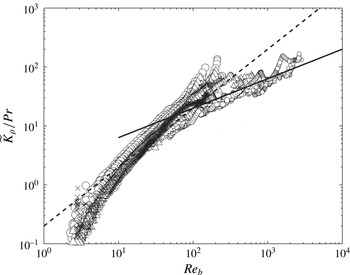
 $K_{{\it\rho}}\propto \mathit{Re}_{b}^{1/2}$
, which according to (2.23) evidently implies
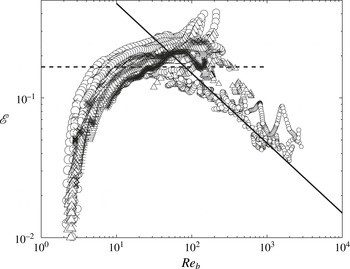
 ${\it\Gamma}\propto \mathit{Re}_{b}^{-1/2}$
. This latter implication has also been empirically noted by SKIF using
 $R_{f}$
as a measure of mixing efficiency. Furthermore, Lozovatsky & Fernando (Reference Lozovatsky and Fernando2012), based on their observational data with
 $\mathit{Re}_{b}>10^{4}$
for stratified flow of the atmospheric surface boundary layer, also suggested a
 $-1/2$
power-law relation between
 $R_{f}$
and
 $\mathit{Re}_{b}$
. We will return to the discussion of such power-law relations in § 4.3.
3. Momentum diffusivity and turbulent Prandtl number
The momentum diffusivity
 $K_{m}$
(also commonly referred to as the eddy viscosity) is conventionally defined as the ratio of the Reynolds stress (turbulent momentum flux) to the vertical shear following the mixing length ansatz as (cf. (2.1)):
 $$\begin{eqnarray}\widetilde{K}_{m}^{ml}=-\frac{1}{{\it\nu}}\frac{\langle \overline{u^{\prime }w^{\prime }}\rangle }{\langle \text{d}\overline{u}/\text{d}z\rangle },\end{eqnarray}$$
in which
 $\widetilde{K}_{m}=K_{m}/{\it\nu}$
is non-dimensionalized by the kinematic viscosity
 ${\it\nu}$
.
Similar to Osborn (Reference Osborn1980) who derived an expression for scalar diffusivity (2.5) (as reviewed in § 2.1.2), Crawford (Reference Crawford1982) also employed the simplified TKE equation and derived a formulation for momentum diffusivity (denoted by
 $K_{m}^{Cr}$
) based on its definition in (3.1) by employing the flux Richardson number, denoted
 $R_{f}$
, to replace the momentum flux term. In dimensionless form, this formulation can be represented as:
 $$\begin{eqnarray}\widetilde{K}_{m}^{Cr}=\left(\frac{1}{1-R_{f}}\right)\frac{{\it\varepsilon}_{k}}{{\it\nu}S^{2}}=\left(\frac{1}{1-R_{f}}\right)\mathit{Ri}_{b}\mathit{Re}_{b},\end{eqnarray}$$
where
 $\mathit{Ri}_{b}=N^{2}/S^{2}$
denotes the vertically averaged gradient Richardson number.
As pointed out recently by Venayagamoorthy & Stretch (Reference Venayagamoorthy and Stretch2010), these formulations of
 $K_{m}$
include reversible contributions to the momentum fluxes in the production terms of the TKE equation and therefore do not represent
 $K_{m}$
with adequate precision. In order to address this issue in the context of statistically homogeneous sheared and stratified turbulence, Venayagamoorthy & Stretch (Reference Venayagamoorthy and Stretch2010) also employed the simplified balance equation of TKE by assuming stationary turbulence as in Crawford (Reference Crawford1982) (i.e.
 $\mathbb{P}=\mathbb{B}+{\it\varepsilon}_{k}$
as discussed in § 2.1.2), but they replaced the buoyancy flux term in terms of
 $K_{{\it\rho}}^{ml}$
as defined in (2.1). In order to extend their expression for
 $K_{m}$
to non-stationary homogeneous flows, they simply replaced
 $K_{{\it\rho}}^{ml}$
with
 $K_{{\it\rho}}^{cox}$
(the latter is defined in (2.6), which becomes identical to
 $K_{{\it\rho}}^{\ast }$
in (2.7) for the special case of homogeneous turbulence as discussed in Venayagamoorthy & Stretch Reference Venayagamoorthy and Stretch2006). In what follows, we will nevertheless address this issue by following a different and more generic approach.
3.1. A revised formulation of momentum diffusivity
$K_{m}$

Our aim in this subsection is to propose a new expression for
 $K_{m}$
(denoted by
 $K_{m}^{\ast }$
) which distinguishes between reversible and irreversible contributions to the momentum diffusivity of a Boussinesq turbulent flow; a distinction which is essential to properly defining this quantity. For this purpose we note that the total energy that is extracted from the mean flow due to a turbulent mixing event, with a rate
 $\mathbb{P}$
, is either retained in the system even after the turbulence decays (we define this component as the ‘reversible’ component,
 $\mathbb{P}_{r}$
, because it is capable in principle of initiating further mixing events) or is eventually dissipated irreversibly into internal energy (denoted by
 $\mathbb{P}_{i}$
). This decomposition can be written as:
 $$\begin{eqnarray}\mathbb{P}=\mathbb{P}_{r}+\mathbb{P}_{i},\end{eqnarray}$$
in which
 $\mathbb{P}$
is associated with the shear production term in the TKE equation due to the interaction between the Reynolds stresses and the mean and fluctuating components of the flow as defined in (2.2).
To further establish the definition of
 $\mathbb{P}_{i}$
and
 $\mathbb{P}_{r}$
in (3.3), we invoke a Reynolds decomposition of the total kinetic energy reservoir
 $\mathscr{K}=\langle \overline{\boldsymbol{u}\boldsymbol{\cdot }\boldsymbol{u}}\rangle /2$
, into its background mean
 $\overline{\mathscr{K}}=\langle \overline{u}^{2}\rangle /2$
and turbulent
 $\mathscr{K}^{\prime }=\langle \overline{\boldsymbol{u}^{\prime }\boldsymbol{\cdot }\boldsymbol{u}^{\prime }}\rangle /2$
components, as well as the decomposition of total potential energy into APE and BPE as discussed in § 2.2, i.e.
 $$\begin{eqnarray}\displaystyle & \mathscr{K}=\overline{\mathscr{K}}+\mathscr{K}^{\prime }, & \displaystyle\end{eqnarray}$$
 $$\begin{eqnarray}\displaystyle & \mathscr{P}=\mathscr{P}_{A}+\mathscr{P}_{B}. & \displaystyle\end{eqnarray}$$
Furthermore, the evolution equations for the energy budgets associated with
 $\mathscr{K}$
,
 $\mathscr{K}^{\prime }$
and
 $\mathscr{P}_{A}$
may be written as (Caulfield & Peltier Reference Caulfield and Peltier2000):
 $$\begin{eqnarray}\displaystyle & \displaystyle \frac{\text{d}}{\text{d}t}\mathscr{K}=-\mathbb{B}-{\it\varepsilon}_{k}, & \displaystyle\end{eqnarray}$$
 $$\begin{eqnarray}\displaystyle & \displaystyle \frac{\text{d}}{\text{d}t}\mathscr{K}^{\prime }=-\mathbb{B}+\mathbb{P}-{\it\varepsilon}_{k}^{\prime }, & \displaystyle\end{eqnarray}$$
 $$\begin{eqnarray}\displaystyle & \displaystyle \frac{\text{d}}{\text{d}t}\mathscr{P}_{A}=\mathbb{B}-\mathscr{M}, & \displaystyle\end{eqnarray}$$
 ${\it\varepsilon}_{k}^{\prime }=2{\it\nu}\overline{\langle \unicode[STIX]{x1D634}_{ij}^{\prime }\unicode[STIX]{x1D634}_{ij}^{\prime }\rangle }$
(cf. (2.4)) and
 $\unicode[STIX]{x1D634}_{ij}^{\prime }=(\partial u_{i}^{\prime }/\partial x_{j}+\partial u_{j}^{\prime }/\partial x_{i})/2$
is the disturbance strain rate tensor.
The ‘irreversible’ component of the shear production,
 $\mathbb{P}_{i}$
, is identified by considering the evolution equation for the total available energy,
 $E_{A}=\mathscr{K}+\mathscr{P}_{A}$
, namely:
 $$\begin{eqnarray}\frac{\text{d}}{\text{d}t}E_{A}=\frac{\text{d}}{\text{d}t}(\mathscr{K}+\mathscr{P}_{A})=-(\mathscr{M}+{\it\varepsilon}_{k}).\end{eqnarray}$$
The above equation implies that the total energy that is available for irreversible mixing at larger scales of motion, in the form of both total kinetic energy and APE, must dissipate at the smallest scales due to either (i) viscous dissipation of fluid filaments
 $({\it\varepsilon}_{k})$
or (ii) a diffusive destruction of small-scale density variance and therefore of potential energy (
 ${\it\varepsilon}_{p}$
). Here we have exploited the fact that
 ${\it\varepsilon}_{p}=\mathscr{M}$
for incompressible Boussinesq flows as explained in § 2.2 (see Tailleux Reference Tailleux2009 for further discussion).
We therefore attribute the irreversible monotonic decrease of
 $E_{A}$
in (3.9) to the irreversible component of shear production,
 $\mathbb{P}_{i}$
, that is manifested at dissipation scales. Thus
 $\mathbb{P}_{i}$
is defined as:
 $$\begin{eqnarray}\mathbb{P}_{i}=\mathscr{M}+{\it\varepsilon}_{k}.\end{eqnarray}$$
Furthermore, the ‘reversible’ component of the shear production,
 $\mathbb{P}_{r}$
, is identified by considering the energy budget of the stratified turbulence (defined as the sum of TKE and APE, see Smyth, Carpenter & Lawrence Reference Smyth, Carpenter and Lawrence2007), which evolves based on the following equation:
 $$\begin{eqnarray}\frac{\text{d}}{\text{d}t}(\mathscr{K}^{\prime }+\mathscr{P}_{A})=-\mathscr{M}-{\it\varepsilon}_{k}^{\prime }+\mathbb{P}.\end{eqnarray}$$
By employing (3.3) and (3.10) and after adding and subtracting mean flow viscous dissipation
 $\overline{{\it\varepsilon}}={\it\nu}\langle (\text{d}\overline{u}/\text{d}z)^{2}\rangle ={\it\varepsilon}_{k}-{\it\varepsilon}_{k}^{\prime }$
, the reversible shear production,
 $\mathbb{P}_{r}$
, is defined as:
 $$\begin{eqnarray}\mathbb{P}_{r}=\frac{\text{d}}{\text{d}t}(\mathscr{P}_{A}+\mathscr{K}^{\prime })-\overline{{\it\varepsilon}}.\end{eqnarray}$$
In other words, the reversible component of
 $\mathbb{P}$
is the rate of change in the sum of APE and TKE reservoirs due to the reversible energy transfer to the mean flow kinetic energy after subtracting the irreversible dissipation of mean flow kinetic energy (
 $\overline{{\it\varepsilon}}$
), because the latter is supplied by the irreversible component of
 $\mathbb{P}$
. Therefore the energy that was noted earlier as being retained after a mixing event is completed, is only associated with the mean flow kinetic energy that is capable of initiating further mixing events. In addition, notice that
 $\mathbb{P}_{r}$
does not contribute to the irreversible loss of
 $E_{A}$
in (3.9). It, rather, contributes to the reversible energy exchanges between the APE–TKE energy reservoir and the mean flow kinetic energy (
 $\overline{\mathscr{K}}$
).
For characterizing
 $K_{m}^{\ast }$
, only the irreversible component of such shear production (i.e.
 $\mathbb{P}_{i}$
), must be employed, whereby
 $K_{m}^{\ast }$
is defined as:
 $$\begin{eqnarray}\widetilde{K}_{m}^{\ast }=\frac{\mathbb{P}_{i}}{{\it\nu}S^{2}}.\end{eqnarray}$$
Similar to the general definition of
 $K_{{\it\rho}}$
in (1.1),
 $K_{m}$
may also be defined as the ratio of a ‘flux’ to a ‘gradient’ (with a negative sign). Therefore (3.13) is obtained by considering
 $-\mathbb{P}_{i}/S$
as the appropriate irreversible momentum ‘flux’ and the vertical shear
 $S$
, as the required ‘gradient’.
Given the definition of
 $\mathbb{P}_{i}$
in (3.10), there are two alternative ways of incorporating previous concepts regarding irreversible mixing of the scalar field into the definition of
 $\widetilde{K}_{m}^{\ast }$
. First, by employing the definition of irreversible mixing efficiency in (2.22),
 $\mathbb{P}_{i}$
may be re-written as:
 $$\begin{eqnarray}\mathbb{P}_{i}=\frac{{\it\varepsilon}_{k}}{1-\mathscr{E}}.\end{eqnarray}$$
Second, by evoking the relationship between
 $\mathscr{M}$
and
 ${\it\phi}_{d}$
in (2.21) and recalling the definition of
 $\widetilde{K}_{{\it\rho}}^{\ast }$
in (2.23), which effectively implies
 $\widetilde{K}_{{\it\rho}}^{\ast }=\mathscr{M}/({\it\kappa}N_{\ast }^{2})$
,
 $\mathbb{P}_{i}$
may be alternatively expressed as:
 $$\begin{eqnarray}\mathbb{P}_{i}=({\it\kappa}N_{\ast }^{2})\widetilde{K}_{{\it\rho}}^{\ast }+{\it\varepsilon}_{k},\end{eqnarray}$$
in which
 $N_{\ast }^{2}$
is again defined based on the adiabatically sorted density profile.
The above two expressions for
 $\mathbb{P}_{i}$
in (3.14) and (3.15) are identical. Nonetheless we have provided both forms because each manipulation has been exploited previously in Crawford (Reference Crawford1982) and Venayagamoorthy & Stretch (Reference Venayagamoorthy and Stretch2010) with certain limitations in each case as reviewed earlier. In what follows we will use each of these alternative forms of
 $\mathbb{P}_{i}$
to derive corresponding alternative expressions for
 $\widetilde{K}_{m}^{\ast }$
based on (3.13) which facilitates comparison with the previous formulae of Crawford (Reference Crawford1982) and Venayagamoorthy & Stretch (Reference Venayagamoorthy and Stretch2010).
By employing
 $\mathbb{P}_{i}$
based on either (3.14) or (3.15),
 $\widetilde{K}_{m}^{\ast }$
may be written in dimensionless form as either of the following expressions:
 $$\begin{eqnarray}\displaystyle \widetilde{K}_{m}^{\ast }=\left(\frac{1}{1-\mathscr{E}}\right)\frac{{\it\varepsilon}_{k}}{{\it\nu}S^{2}}, & & \displaystyle\end{eqnarray}$$
 $$\begin{eqnarray}\displaystyle \widetilde{K}_{m}^{\ast }=\left(\frac{\mathit{Ri}_{b}^{\ast }}{\mathit{Pr}}\right)\widetilde{K}_{{\it\rho}}^{\ast }+\frac{{\it\varepsilon}_{k}}{{\it\nu}S^{2}}, & & \displaystyle\end{eqnarray}$$
in which
 $Ri_{b}^{\ast }=N_{\ast }^{2}/S^{2}$
is defined based on the sorted background density profile. Obviously, by equating
 $\widetilde{K}_{m}^{\ast }$
based on (3.16) and (3.17), the revised expression for
 $\widetilde{K}_{{\it\rho}}^{\ast }$
in (2.23) is obtained.
It is important to note that (3.16) closely resembles the formulation of Crawford (Reference Crawford1982) in (3.2) except for the following critical differences. (i) The new formula for
 $K_{m}$
employs the correct definition of mixing efficiency
 $\mathscr{E}$
rather than the flux Richardson number
 $R_{f}$
(refer to Peltier & Caulfield Reference Peltier and Caulfield2003 and Tailleux Reference Tailleux2009 for a discussion of the intrinsic differences between
 $\mathscr{E}$
and
 $R_{f}$
). Moreover, (ii) the expression for
 $K_{m}$
in (3.16) does not involve any assumptions concerning the flow dynamics, as opposed to (3.2) which is derived based on the same limitations as those of the Osborn formula for
 $K_{{\it\rho}}$
.
In addition, (3.17) also closely resembles the homogeneous formulation of Venayagamoorthy & Stretch (Reference Venayagamoorthy and Stretch2010) (see their equation (2.8)) although it significantly extends their expression to any inhomogeneously stratified Boussinesq flow at sufficiently high
 $\mathit{Re}$
.
3.2. Turbulent Prandtl number
$\mathit{Pr}_{t}$

A non-dimensional parameter of fundamental concern is the ratio of turbulent momentum diffusivity to the diapycnal diffusivity of density as characterized by the turbulent Prandtl number
 $\mathit{Pr}_{t}=K_{m}/K_{{\it\rho}}$
. Using the newly proposed expressions for
 $K_{{\it\rho}}$
in (2.23) and for
 $K_{m}$
in (3.16),
 $\mathit{Pr}_{t}$
becomes:
 $$\begin{eqnarray}\mathit{Pr}_{t}=\frac{\mathit{Ri}_{b}}{\mathscr{E}}.\end{eqnarray}$$
In the absence of careful definitions for
 $K_{{\it\rho}}$
and
 $K_{m}$
,
 $\mathit{Pr}_{t}$
is commonly defined as the ratio of
 $K_{m}^{ml}$
in (3.1) to
 $K_{{\it\rho}}^{ml}$
in (2.1) based on the mixing length argument, which results in
 $\mathit{Pr}_{t}^{\,ml}=\mathit{Ri}_{b}/R_{f}$
. The new expression for
 $\mathit{Pr}_{t}$
in (3.18) also resembles this basic definition of turbulent Prandtl number except that
 $\mathscr{E}$
appears in place of
 $R_{f}$
. As a result of this slight but important modification,
 $\mathit{Pr}_{t}$
represents only the ratio of irreversible components of scalar and momentum diffusivities, which again critically depends on the accurate definition of irreversible mixing efficiency.
4. Direct numerical simulations of inhomogeneously stratified, shear-generated turbulence
In this second part of the paper, we will illustrate the results obtained using the newly proposed formulations for
 $K_{{\it\rho}}$
,
 $K_{m}$
and
 $\mathit{Pr}_{t}$
, and in the case of
 $K_{{\it\rho}}$
will compare this with the complete set of models we have reviewed. A large dataset of original DNS results associated with the KH ansatz will be employed to achieve this goal. First, in § 4.1 we describe our choice of problem configuration as well as the numerical methodology to be employed. The results obtained on the basis of these analyses are then consolidated in §§ 4.2–4.5. In appendix A, we will comment on the other model problem that has been employed for the study of shear-induced turbulence in stratified flows (e.g. in SKIF), which is referred to as homogeneous stratified and sheared turbulence.
4.1. Design of the suite of DNS analyses
Our intention is to provide a detailed investigation of the stratified turbulence that is generated through the transition of a primary shear instability in the form of a Kelvin–Helmholtz wave which thereafter ‘breaks’ to generate the turbulence of interest. As initial conditions, the velocity and density fields are set to the following one-dimensional initial profiles:
 $$\begin{eqnarray}\overline{U}_{0}(z)=U_{0}\tanh \left(\frac{z}{d}\right),\quad \overline{{\it\rho}}_{0}(z)={\it\rho}_{0}-{\rm\Delta}{\it\rho}\tanh \left(\frac{z}{d}\right),\end{eqnarray}$$
which are both assumed to have equal thickness
 $2d$
. Also
 $U_{0}$
and
 ${\it\rho}_{0}$
denote a reference velocity and density while
 ${\rm\Delta}{\it\rho}$
describes a fixed density difference across the shear layer. The coordinate system is chosen such that
 $x,y$
and
 $z$
are aligned with the streamwise, spanwise and vertical directions respectively.
We non-dimensionalize the governing Boussinesq equations in (2.9)–(2.11) by choosing
 ${\it\rho}_{0}$
,
 $U_{0}$
and
 $d$
(half of the shear layer thickness) as the characteristic density, velocity and length scales which become:
 $$\begin{eqnarray}\displaystyle & \displaystyle \frac{\text{D}u_{i}}{\text{D}t}=-\frac{\partial p}{\partial x_{i}}-\mathit{Ri}_{0}{\it\rho}{\it\delta}_{i3}+\frac{1}{\mathit{Re}}\frac{\partial ^{2}u_{i}}{\partial x_{j}^{2}}, & \displaystyle\end{eqnarray}$$
 $$\begin{eqnarray}\displaystyle & \displaystyle \frac{\partial u_{i}}{\partial x_{i}}=0, & \displaystyle\end{eqnarray}$$
 $$\begin{eqnarray}\displaystyle & \displaystyle \frac{\text{D}{\it\rho}}{\text{D}t}=\frac{1}{\mathit{Re}\,\mathit{Pr}}\frac{\partial ^{2}{\it\rho}}{\partial x_{j}^{2}}. & \displaystyle\end{eqnarray}$$
 $$\begin{eqnarray}\mathit{Re}=\frac{U_{0}d}{{\it\nu}},\quad \mathit{Ri}=-\frac{g}{{\it\rho}_{0}}\frac{\partial {\it\rho}}{\partial z}\left(\frac{\partial u}{\partial z}\right)^{-2},\quad \mathit{Pr}=\frac{{\it\nu}}{{\it\kappa}}.\end{eqnarray}$$
The minimum value in the initial profile of
 $Ri$
(not to be confused with its vertically averaged bulk measure defined in (1.2) as
 $\mathit{Ri}_{b}$
), obtained from the initial density and velocity profiles in (4.1), occurs at the inflection point of the velocity profile (located at
 $z=0$
). We will denote this specific choice of gradient Richardson number by
 $\mathit{Ri}_{0}$
, which appears as the coefficient of the non-dimensional buoyancy term in (2.9). We also retain our non-dimensional representations of diapycnal diffusivity and momentum diffusivity as introduced in the previous section, namely
 $\widetilde{K}_{{\it\rho}}=K_{{\it\rho}}/{\it\kappa}$
and
 $\widetilde{K}_{m}=K_{m}/{\it\nu}$
in which
 ${\it\kappa}={\it\nu}/\mathit{Pr}$
and
 ${\it\nu}=U_{0}d/\mathit{Re}$
based on our choice of
 $\mathit{Pr}$
and
 $\mathit{Re}$
in the non-dimensionalized Boussinesq equations. We also note in passing that it is common practice in the oceanographic literature (e.g. Smyth et al.
Reference Smyth, Moum and Caldwell2001) to choose
 $2{\it\rho}_{0}$
,
 $2U_{0}$
and
 $2d$
as the characteristic density, velocity and length scales for the non-dimensionalization. Therefore our
 $\mathit{Re}$
should be multiplied by four in order to make direct comparisons to these earlier studies.
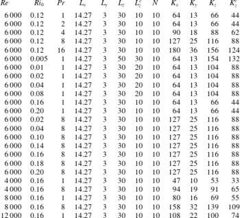
The DNS-based analysis of stratified turbulent flows to be discussed in the main body of this paper include those reported in Salehipour, Peltier & Mashayek (Reference Salehipour, Peltier and Mashayek2015) (with
 $\mathit{Re}=6000$
,
 $\mathit{Ri}_{0}=0.12$
and
 $\mathit{Pr}=1,2,4,8,16$
) as well as an additional series of new simulations which are all listed in table 1. In the subset of these simulations discussed in Salehipour et al. (Reference Salehipour, Peltier and Mashayek2015), the focus was upon variations in the molecular Prandtl number at a fixed Reynolds number of
 $\mathit{Re}=6000$
and a fixed minimum initial gradient Richardson number (at the inflection point) of
 $\mathit{Ri}_{0}=0.12$
. The new set of simulations includes various
 $\mathit{Ri}_{0}$
at a fixed
 $\mathit{Re}$
and
 $\mathit{Pr}$
(
 $\mathit{Re}=6000$
,
 $\mathit{Pr}=1,8$
) and various
 $\mathit{Re}$
at a fixed
 $\mathit{Ri}_{0}$
and
 $\mathit{Pr}~(\mathit{Ri}_{0}=0.16,\mathit{Pr}=1,8)$
. All these simulations have been performed using the modern spectral element code, Nek5000, developed at the Argonne National Laboratory (Fischer, Kruse & Loth Reference Fischer, Kruse and Loth2002; Fischer, Lottes & Kerkemeier Reference Fischer, Lottes and Kerkemeier2008). The governing Navier–Stokes equations are discretized using the weak Galerkin formulation by employing
 $N$
th-order Lagrange polynomial interpolants following the
 $P_{N}-P_{N-2}$
formulation of Maday, Patera & Rønquist (Reference Maday, Patera and Rønquist1990) for the velocity (
 $N$
) and pressure (
 $N-2$
) spaces respectively. In terms of the temporal discretization, a third-order semi-implicit operator-splitting method is employed (Maday et al.
Reference Maday, Patera and Rønquist1990; Fischer Reference Fischer1997). Besides higher-order accuracy, this code is ideally suited for our high-
 $\mathit{Re}$
, high-
 $\mathit{Pr}$
numerically demanding simulations due to its perfect scaling up to thousands of processors (we have successfully employed up to 65 536 cores on a BlueGene/Q machine). Table 1 also includes the streamwise (
 $L_{x}$
), spanwise (
 $L_{y}$
) and vertical (
 $L_{z}$
) extents of the computational domain as well as the number of elements in each direction (i.e.
 $K_{x},K_{y},K_{z}$
). The domain is periodic in the
 $x$
and
 $y$
directions, while the top and bottom boundaries are assumed to be free-slip and impermeable for velocity and insulated (zero density flux) for the density field. For further details concerning the numerical set-up, grid design, domain size, resolution requirements and initial perturbations the interested reader is referred to Salehipour et al. (Reference Salehipour, Peltier and Mashayek2015).
Details of the three-dimensional numerical experiments in which the total grid points is about
 $N^{3}K_{x}K_{y}K_{z}$
. Also,
 $L_{z}^{c}$
represents the height of a central region of the domain which is further refined with
 $K_{z}^{c}$
elements. Outside
 $L_{z}^{c}$
, the adjacent elements of the grid are gradually stretched by a factor of 1.25 %.

For all the figures to be presented in this paper, we have adopted a special annotation to differentiate between the simulations that have different
 $\mathit{Pr}$
and
 $\mathit{Ri}_{b}$
. All the runs at
 $\mathit{Pr}=1$
are marked by a circle (○) while those at
 $\mathit{Pr}=8$
are shown by a triangle (▵). Single runs at
 $\mathit{Pr}=2,4,16$
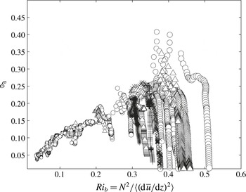
are also shown respectively by ×, + and ∗. Furthermore, the marker size was chosen to approximately represent the vertically averaged gradient Richardson number,
 $\mathit{Ri}_{b}$
, such that lower
 $\mathit{Ri}_{b}$
corresponds to smaller symbols. These distinctions are not intended to delineate these runs, but rather to facilitate our discussions to follow.
Unless otherwise stated explicitly, in all the results to be discussed in what follows the bulk measure of the gradient Richardson number,
 $\mathit{Ri}_{b}$
, will be calculated as
 $\mathit{Ri}_{b}=N^{2}/\langle (\text{d}\overline{u}/\text{d}z)^{2}\rangle$
(i.e. vertical shear is first squared and then vertically averaged) in which
 $N^{2}=-\mathit{Ri}_{0}\langle \text{d}\overline{{\it\rho}}/\text{d}z\rangle =\mathit{Ri}_{0}{\rm\Delta}{\it\rho}/L_{z}$
due to our non-dimensionalization. Appendix B compares this preferred form of
 $\mathit{Ri}_{b}$
with an alternative definition for
 $\mathit{Ri}_{b}$
in which shear is first vertically averaged over the shear layer and then squared. Based on all of the DNS cases, an empirical relationship between the two definitions is also suggested in appendix B, which may serve as a mapping function between these two forms of
 $\mathit{Ri}_{b}$
.
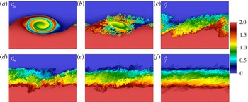
Figure 1 illustrates an example DNS analysis in which the density field for a case with
 $\mathit{Re}=6000$
,
 $\mathit{Pr}=8$
and
 $\mathit{Ri}_{0}=0.16$
is shown in different panels corresponding to different snapshots of time during flow evolution. Note that the time-dependent flow field undergoes various stages of evolution, beginning with the growth of the two-dimensional Kelvin–Helmholtz instability whose kinetic energy saturates at a time denoted by
 $t_{2d}^{s}$
in figure 1(a). The onset of the fully turbulent regime does not begin until
 $t_{f}^{o}>t_{2d}^{s}$
, at which time the kinetic energy of inherently three-dimensional flow components finally exceeds that of the two-dimensional flow (figure 1
c). For the time period of
 $t_{2d}^{s}<t<t_{f}^{o}$
(figure 1
b), three-dimensional secondary instabilities grow and facilitate the transition to turbulence. At a time
 $t_{3d}^{s}>t_{f}^{o}$
, three-dimensional kinetic energy has saturated relative to the two-dimensional flow component and thus there is hardly any visible signature of the original two-dimensional KH wave in the flow field (figure 1
d). We have realized that it is critical not to define
 $t_{3d}^{s}$
as the time when the kinetic energy of the three-dimensional flow is highest because this point may occur when the kinetic energy of the two-dimensional KH wave continues to overwhelm that of the induced three-dimensional turbulence and is therefore not associated with the fully turbulent phase. The period of sustained or decaying turbulence ends at a time denoted by
 $t_{f}^{e}$
, which we have chosen to define based on a threshold minimum
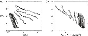
 $\mathit{Re}_{b}$
. The flow field begins to re-laminarize (figure 1
f), usually around
 $\mathit{Re}_{b}=20$
in agreement with previous suggestions in the literature (e.g. see Stillinger, Helland & Atta Reference Stillinger, Helland and Van Atta1983; Smyth & Moum Reference Smyth and Moum2000b
). For the purpose of all of the analyses to be discussed in this paper,
 $t_{f}^{e}$
is, rather, defined based on a threshold minimum value of
 $\mathit{Re}_{b}=1$
in order to also encompass the mixing properties of weakly turbulent flows with extremely low
 $\mathit{Re}_{b}$
. In addition, we will entirely focus upon the period of fully turbulent flow (i.e.
 $t_{3d}^{s}\leqslant t\leqslant t_{f}^{e}$
, depicted in figure 1
d–f) in order to calculate mixing efficiency as well as the scalar and momentum diffusivities.
Illustrations of density field evolution. Streamwise-vertical cross-section at the mid-point in the cross-stream
 $y$
direction for different time snapshots
 $t_{2d}^{s}$
,
 $t\in [t_{2d}^{s}\quad t_{f}^{o}]$
,
 $t_{3d}^{s}$
,
 $t\in [t_{3d}^{s}\quad t_{f}^{e}]$
and
 $t_{f}^{e}$
. For the definition of these times refer to the text.

In terms of the non-dimensional control parameters,
 $D_{p}$
(as introduced in § 2.2) may be rewritten as
 $D_{p}=\mathit{Ri}_{0}{\rm\Delta}{\it\rho}/(\mathit{Re}\mathit{Pr}L_{z})$
where
 $L_{z}$
is the vertical extent of the computational domain. In all the DNS cases tabulated in table 1,
 ${\rm\Delta}{\it\rho}=2$
,
 $L_{z}=30$
,
 $\mathit{Ri}_{0}\sim O(10^{-1}{-}10^{-2})$
,
 $\mathit{Pr}\sim O(10^{0}{-}10^{1})$
and
 $\mathit{Re}\sim O(10^{3}{-}10^{4})$
. Thus
 $D_{p}\sim O(10^{-9}{-}10^{-6})$
, which is two to five orders of magnitude smaller than the irreversible mixing,
 $\mathscr{M}$
, that is usually of order
 $\mathscr{M}\sim O(10^{-4})$
(also non-dimensional). During the final stages of the KH life cycle however, the flow begins to re-laminarize and turbulent mixing decays to zero (i.e.
 $\mathscr{M}\sim D_{p}\sim 0$
when
 $\mathit{Re}_{b}\sim O(10^{0}{-}10^{1})$
). This may seem to suggest that the revised formulation for
 $\widetilde{K}_{{\it\rho}}$
in (2.23) might not be applicable because (2.18) is not strictly satisfied when
 $\mathscr{M}\sim D_{p}$
. Nevertheless, since turbulent mixing is negligible during this stage in any event (i.e.
 $\mathscr{M}\sim 0$
), our proposed framework still holds and predicts that both mixing efficiency and diapycnal diffusivity would decay to zero.
4.2. Scalar diffusivity estimation: a comparative study
Different estimations of diapycnal diffusivity
 $K_{{\it\rho}}$
that are commonly employed in the literature will be compared here with the ‘correct’ value of scalar diffusivity
 $K_{{\it\rho}}^{\ast }$
. As discussed in § 2.3, the ‘correct’ formulation of
 $K_{{\it\rho}}^{\ast }$
was proposed in the context of the diascalar framework of WD96 which has been mathematically reformulated in this paper into the form of a more familiar ‘Osborn-like’ expression. Therefore
 $K_{{\it\rho}}^{\ast }$
may be considered to have been calculated based on either method.
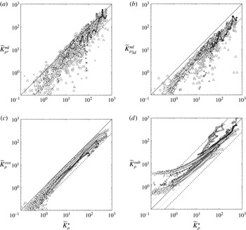
Figure 2 contains the individual comparisons made between each non-dimensional estimation of scalar diffusivity and
 $\widetilde{K}_{{\it\rho}}^{\ast }=K_{{\it\rho}}/{\it\kappa}$
. Figures 2(d) and 2(c) investigate the accuracy of the Osborn (Reference Osborn1980) (with
 $R_{f}=0.17$
or
 ${\it\gamma}=0.2$
, see (2.5)) and Osborn & Cox (Reference Osborn and Cox1972) (see (2.6)) models for estimating diapycnal diffusivity. As far as the mixing length model is concerned,
 $\widetilde{K}_{{\it\rho}}^{ml}$
in (2.1) has been calculated using two alternative assumptions for the perturbation density flux
 $\overline{{\it\rho}^{\prime }w^{\prime }}$
. Namely (i)
 $\widetilde{K}_{{\it\rho}^{\prime }}^{ml}$
in figure 2(a) involves the conventional Reynolds decomposition (
 $f=\overline{f}+f^{\prime }$
) whereas (ii)
 $\widetilde{K}_{{\it\rho}_{3d}}^{ml}$
in figure 2(b) employs a density flux that is only based on the inherently three-dimensional component of a triple Reynolds decomposition (
 $f=\overline{f}+f_{2d}+f_{3d}$
). Here
 $f$
denotes either density or vertical velocity fields and
 $\overline{f}$
isolates the horizontal mean from the
 $2d$
and
 $3d$
components which respectively represent the spanwise averaged and fully three-dimensional components of a flow field (refer to Caulfield & Peltier Reference Caulfield and Peltier2000 for precise definitions).
Comparing the accurate representation of scalar diffusivity
 $\widetilde{K}_{{\it\rho}}^{\ast }$
(2.7) or (2.23) with: (a) mixing length model (2.1) based on a full perturbation buoyancy flux
 $\widetilde{K}_{{\it\rho}^{\prime }}$
or (b) based on inherently three-dimensional buoyancy flux
 $\widetilde{K}_{{\it\rho}_{3d}}$
; (c) the Osborn–Cox model
 $\widetilde{K}_{{\it\rho}}^{cox}$
(2.6); and (d) the Osborn formula
 $\widetilde{K}_{{\it\rho}}^{osb}$
(2.5) (with
 $R_{f}=0.17$
). The dashed (dotted) lines show a factor of four (two) under/over-estimation. See figure 3 caption for description of symbols.

Figure 2 illustrates the fact that the models investigated herein are accurate only within a factor of approximately four. In general, there is a fundamental problem concerning the use of ‘turbulent’ density flux,
 $\overline{{\it\rho}^{\prime }w^{\prime }}$
, in the mixing length model in order to estimate the diapycnal diffusivity. Namely, the density flux in the usual vertical coordinate system would inevitably and improperly include reversible processes in the estimation of
 $K_{{\it\rho}}$
. For example, the direct field measurements of the instantaneous density flux
 $\overline{{\it\rho}^{\prime }w^{\prime }}$
(e.g. Moum Reference Moum1990; Fleury & Lueck Reference Fleury and Lueck1994) attest to the fact that the interpretation of such measurements is non-trivial since this flux becomes as frequently positive (down-gradient) as negative (counter-gradient). Furthermore, figure 16 in Mashayek & Peltier (Reference Mashayek and Peltier2013) shows negative values for
 $K_{{\it\rho}}$
derived on the basis of the use of (2.1) using
 $\overline{{\it\rho}^{\prime }w^{\prime }}$
, which is clearly unphysical. Due to its logarithmic scale, figure 2(a) does not show the negative values of
 $\widetilde{K}_{{\it\rho}^{\prime }}^{ml}$
, but the large scatter away from the correct estimation of diapycnal diffusivity should be seen as indicative of the same fundamental problem. Although use of a triple Reynolds decomposition to obtain
 $\overline{{\it\rho}_{3d}w_{3d}}$
is empirically seen to produce values for this flux which are strictly positive,
 $\widetilde{K}_{{\it\rho}_{3d}}^{ml}$
is still unable to capture the complete irreversible diapycnal flux
 ${\it\phi}_{d}$
as defined in (2.8) or (2.21) because there exists a clear offset between
 $\widetilde{K}_{{\it\rho}_{3d}}^{ml}$
and
 $\widetilde{K}_{{\it\rho}}$
which points to the fact that
 $\overline{{\it\rho}_{3d}w_{3d}}$
systematically underestimates
 ${\it\phi}_{d}$
.
Although the Osborn–Cox model also underestimates the actual scalar diffusivity in figure 2(c), it seems to provide the best estimates among the complete set of approximate models. Not only is
 $\widetilde{K}_{{\it\rho}}^{cox}$
(or the Cox number) close to the actual values of
 $\widetilde{K}_{{\it\rho}}^{\ast }$
(i.e.
 $0.25\widetilde{K}_{{\it\rho}}^{\ast }\leqslant \widetilde{K}_{{\it\rho}}^{cox}\leqslant \widetilde{K}_{{\it\rho}}^{\ast }$
), but it also correctly follows the trend in
 $\widetilde{K}_{{\it\rho}}^{\ast }$
(i.e. the independent series of data points are all individually aligned with the solid line of
 $\widetilde{K}_{{\it\rho}}^{cox}=\widetilde{K}_{{\it\rho}}^{\ast }$
). In fact, the Osborn–Cox estimate would be accurate (within an approximately
 $\pm 50\,\%$
offset), if it were multiplied by a factor of 2. This is based on figure 2(c) in which the DNS data encompass the line
 $\widetilde{K}_{{\it\rho}}^{cox}=0.5\widetilde{K}_{{\it\rho}}^{\ast }$
(dotted line in figure 2
c).
The Osborn model in figure 2(d), on the other hand, does not follow the trend in
 $\widetilde{K}_{{\it\rho}}^{\ast }$
. In fact,
 $\widetilde{K}_{{\it\rho}}^{osb}$
deviates noticeably from the line of
 $\widetilde{K}_{{\it\rho}}^{osb}=\widetilde{K}_{{\it\rho}}^{\ast }$
at both extreme limits of diapycnal diffusivity. This inaccuracy has been commonly remarked upon as being associated with the assumptions employed in the derivation of the Osborn formula (Mashayek, Caulfield & Peltier Reference Mashayek, Caulfield and Peltier2013; Mashayek & Peltier Reference Mashayek and Peltier2013), in addition to the accepted deviations of mixing efficiency from any canonical constant value (e.g. Ivey et al.
Reference Ivey, Winters and Koseff2008). Although geophysical flows do not obey the simplifying assumptions of Osborn (Reference Osborn1980), we showed in § 2.3 that for any Boussinesq stratified fluid with high
 $\mathit{Re}$
, an expression for
 $K_{{\it\rho}}$
similar to the Osborn formula is indeed accurate, provided that
 $\mathscr{E}$
replaces the flux Richardson number
 $R_{f}$
. It is worthwhile noting that, even if a ‘variable’ flux Richardson number were to be used in the Osborn model (2.5), there would still exist an inconsistency between
 $\widetilde{K}_{{\it\rho}}^{osb}$
and
 $\widetilde{K}_{{\it\rho}}^{\ast }$
due to an inherent inability of
 $R_{f}$
to isolate the diabatic process of irreversible mixing from the adiabatic process of reversible stirring (Peltier & Caulfield Reference Peltier and Caulfield2003; Tailleux Reference Tailleux2009). Nonetheless, the major discrepancy between
 $\widetilde{K}_{{\it\rho}}^{osb}$
and
 $\widetilde{K}_{{\it\rho}}^{\ast }$
in figure 2(d) should be ascribed to the assumption of constant mixing efficiency. The issue of constant versus variable mixing efficiency is a pressing one because, based on (2.23),
 $\widetilde{K}_{{\it\rho}}^{\ast }\propto \mathscr{E}/(1-\mathscr{E})$
which indicates that extreme variations of
 $\widetilde{K}_{{\it\rho}}^{\ast }$
will occur in the near vicinity of
 $\mathscr{E}=0$
. This implies that using
 $\mathscr{E}=0.17$
(or
 ${\it\Gamma}=0.2$
) would overestimate
 $\widetilde{K}_{{\it\rho}}^{\ast }$
by several orders of magnitude if the stratified shear flow is being mixed quite inefficiently (e.g. when the flow is either very weakly or highly stratified).
For the remainder of this paper, we will primarily employ the accurate formulation of diapycnal diffusivity
 $\widetilde{K}_{{\it\rho}}^{\ast }$
obtained from either (2.7) or (2.23). To simplify notation, we will drop the asterisk and simply refer to
 $\widetilde{K}_{{\it\rho}}$
as the diapycnal scalar diffusivity. The dimensionless notation (denoted by
 $\widetilde{K}$
) will be retained, which implies division by molecular diffusivity,
 ${\it\kappa}$
, and kinematic viscosity,
 ${\it\nu}$
, for
 $\widetilde{K}_{{\it\rho}}$
and
 $\widetilde{K}_{m}$
respectively.
4.3. Turbulent scalar diffusivity and mixing efficiency
Figure 3 compiles the data derived from all of the simulations whose characteristics have been tabulated in table 1 and illustrates the variations of
 $\widetilde{K}_{{\it\rho}}$
with respect to the buoyancy Reynolds number
 $\mathit{Re}_{b}={\it\varepsilon}_{k}/({\it\nu}N^{2})$
. The data points for each DNS experiment are associated with the fully turbulent phase of the flow evolution which belong to
 $t\in [\begin{array}{@{}cc@{}}t_{3d}^{s} & t_{f}^{e}\end{array}]$
. For the purpose of generating this figure (and the similar figures to be discussed in what follows), as noted in § 4.1 we have computed
 $t_{f}^{e}$
based on
 $\mathit{Re}_{b}=1$
in order to also include the re-laminarized flow whose turbulent diapycnal diffusivity approaches zero. It is important to mention that not all of the DNS runs have achieved
 $\mathit{Re}_{b}=O(10^{0}{-}10^{1})$
. Especially for the weakly stratified cases, in which the turbulence suppressing influence of the buoyancy force is considerably weaker than other more highly stratified situations, the turbulence persists for much longer periods (i.e.
 $t_{f}^{e}\gg t_{3d}^{s}$
). Thus in these cases, as will be illustrated later, the simulations require a much greater expenditure of computational resources in order to allow the full influence of the buoyancy effects to activate so as to significantly diminish the turbulence intensity.
Variation of non-dimensional diapycnal scalar diffusivity
 $\widetilde{K}_{{\it\rho}}=K_{{\it\rho}}/{\it\kappa}$
with the buoyancy Reynolds number
 $\mathit{Re}_{b}={\it\varepsilon}_{k}/{\it\nu}N^{2}$
.
 $\widetilde{K}_{{\it\rho}}$
has been calculated based on (2.7) due to WD96 or our proposed reformulation in (2.23). This figure illustrates a compilation of 24 DNS runs with various combinations of
 $\mathit{Re}$
,
 $\mathit{Ri}_{0}$
and
 $\mathit{Pr}$
as tabulated in table 1 and are all associated with the fully turbulent phase of the flow evolution as defined in the text for the KH ansatz; ○,
 $\mathit{Pr}=1$
; ×,
 $\mathit{Pr}=2$
; +,
 $\mathit{Pr}=4$
; ▵,
 $\mathit{Pr}=8$
;
 $\ast$
,
 $\mathit{Pr}=16$
. Bigger (smaller) markers are associated with higher (lower)
 $\mathit{Ri}_{b}$
. Time increases roughly as
 $\mathit{Re}_{b}$
decreases.

The magnitude of diapycnal diffusivity,
 $K_{{\it\rho}}$
, in the interior of lakes and oceans is typically of
 $O({\it\kappa})$
and
 $O(10^{2}{\it\kappa})$
respectively (Ivey et al.
Reference Ivey, Winters and Koseff2008). These values however increase to
 $O(10^{2}{\it\kappa})$
(for lakes) and
 $O(10^{4}{\it\kappa})$
(for oceans) as we approach abyssal regions with rough topography (Ledwell et al.
Reference Ledwell, Montgomery, Polzin, St. Laurent, Schmitt and Toole2000). In addition, there are other ‘hot spots’, such as coastal zones and equatorial near-surface currents, where
 $K_{{\it\rho}}$
may be as large. The range of our non-dimensionalized diapycnal diffusivity
 $\widetilde{K}_{{\it\rho}}=K_{{\it\rho}}/{\it\kappa}$
in figure 3 reaches
 $O(10^{3})$
due to the higher molecular Prandtl numbers of
 $O(10)$
investigated in this work. For instance, if we take the molecular diffusivity of temperature-stratified seawater as
 ${\it\kappa}_{T}=10^{-7}~\text{m}^{2}~\text{s}^{-1}$
, and its molecular Prandtl number to be
 $\mathit{Pr}=7$
, then the DNS results at
 $\mathit{Pr}=8$
in figure 3 suggest that the range of dimensional turbulent diapycnal diffusivity
 $K_{{\it\rho}}$
reaches approximately
 $K_{{\it\rho}}\approx 10^{-4}~\text{m}^{2}~\text{s}^{-1}$
, which lies within the range of estimated turbulent diffusivities in the ocean (Waterhouse et al.
Reference Waterhouse, MacKinnon, Nash, Alford, Kunze, Simmons, Polzin, St. Laurent, Sun, Pinkel, Talley, Whalen, Huussen, Carter, Fer, Waterman, Naveira Garabato, Sanford and Lee2014).
It is useful to compare our DNS results for
 $K_{{\it\rho}}$
with those reported in figure 1 of SKIF. Based on their numerical results, SKIF categorized the turbulent mixing into three regimes in terms of
 $\mathit{Re}_{b}$
: (i) a ‘molecular’ regime for
 $\mathit{Re}_{b}<7$
, (ii) an ‘intermediate’ regime corresponding to stationary turbulence for
 $7<\mathit{Re}_{b}<100$
and (iii) an ‘energetic’ regime for
 $\mathit{Re}_{b}>100$
. Note that the DNS results of SKIF are based on a constant value of
 $\mathit{Pr}=0.72$
whereas figure 3 includes DNS runs with various
 $\mathit{Pr}$
. Thus we have normalized
 $\widetilde{K}_{{\it\rho}}$
by
 $\mathit{Pr}$
in figure 4, thereby effectively plotting
 $K_{{\it\rho}}/{\it\nu}$
(where
 $K_{{\it\rho}}$
is dimensional) versus
 $\mathit{Re}_{b}$
. Despite the intrinsic differences between the geophysically relevant flows we are analysing (e.g. see Smyth et al.
Reference Smyth, Moum and Caldwell2001 for a discussion concerning such relevance) and the more highly constrained homogeneous problem of SKIF and their calculation methodology for
 $K_{{\it\rho}}$
(which is based on the mixing length model), there exist striking similarities between our figure 4 and their figure 1. In order to better highlight the similarities, figure 4 also includes the approximation of diapycnal diffusivity due to Osborn (Reference Osborn1980),
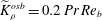 $\widetilde{K}_{{\it\rho}}^{osb}=0.2\,\mathit{Pr}\,\mathit{Re}_{b}$
, as discussed in § 2.1.2 (shown by a dashed line), as well as the line of best fit taken from SKIF for their ‘energetic’ regime, namely
 $\widetilde{K}_{{\it\rho}}=2\,\mathit{Pr}\,\mathit{Re}_{b}^{1/2}$
(shown by a solid line).
Variation of non-dimensional diapycnal scalar diffusivity
 $\widetilde{K}_{{\it\rho}}$
(after being normalized by
 $\mathit{Pr}$
) with
 $\mathit{Re}_{b}={\it\varepsilon}_{k}/{\it\nu}N^{2}$
for all of the DNS cases investigated. – – –, Osborn formula of
 $\widetilde{K}_{{\it\rho}}=0.2\,\mathit{Pr}\,\mathit{Re}_{b}$
(2.5); ——,
 $\widetilde{K}_{{\it\rho}}=2\,\mathit{Pr}\,\mathit{Re}_{b}^{1/2}$
best fit in SKIF. For symbol conventions, refer to figure 3.

Similar to SKIF, a transition to a noticeably different regime of turbulent mixing is also evident in our simulations at approximately
 $\mathit{Re}_{b}=O(10^{2})$
. However, unlike SKIF, our data that reside in the range of
 $7<\mathit{Re}_{b}<100$
are associated with dynamically evolving flow fields that bear minimal resemblance to ‘stationary’ turbulence (e.g. see our figure 1). In fact, our results show that the major difference between DNS cases whose
 $\mathit{Re}_{b}$
exceeds 100 and those below
 $\mathit{Re}_{b}\approx 100$
is associated with their stratification level. The onset of turbulence for the ‘weakly stratified’ simulations with the minimum initial Richardson numbers of
 $\mathit{Ri}_{0}=5\times 10^{-3}$
,
 $1\times 10^{-2}$
and
 $2\times 10^{-2}$
(at
 $\mathit{Pr}=1$
and
 $\mathit{Re}=6000$
), occurs well above
 $\mathit{Re}_{b}=100$
, while most of the other runs that are relatively more ‘strongly stratified’ belong to the regime with
 $\mathit{Re}_{b}<100$
. For these reasons, it is more instructive to denote the ‘intermediate’ and ‘energetic’ regimes of SKIF respectively as corresponding to ‘buoyancy-dominated’ and ‘shear-dominated’ mixing regimes based on the competing dominance of density stratification and velocity shear as characterized by
 $\mathit{Ri}_{b}$
. Furthermore, the ‘molecular’ regime in which molecular diffusion dominates the turbulent diffusion (i.e.
 $\widetilde{K}_{{\it\rho}}<1$
) seems to occur at
 $\mathit{Re}_{b}=O(10^{0})$
, with
 $\mathit{Re}_{b}=7$
as a reasonable characteristic value (in agreement with SKIF) for the transition from the ‘molecular’ regime to the ‘buoyancy-dominated’ regime.
None of the above transition points should be regarded as precise because a transition from one regime of mixing to another would be expected to occur smoothly. For example, Bouffard & Boegman (Reference Bouffard and Boegman2013) suggested a new
 $\mathit{Pr}$
-dependent regime between the ‘molecular’ and the ‘intermediate’ regimes of SKIF in which the diapycnal diffusivity varies with a different slope of
 $\mathit{Re}_{b}^{3/2}$
. Our DNS results also support this slight change in the slope for this limited range of
 $\mathit{Re}_{b}$
(especially for the higher-
 $\mathit{Pr}$
simulations). However, we believe that any careful attempt to estimate the variations of
 $\widetilde{K}_{{\it\rho}}/\mathit{Pr}$
in figure 4 in terms of a power-law relation (i.e.
 $\widetilde{K}_{{\it\rho}}/\mathit{Pr}\propto \mathit{Re}_{b}^{{\it\alpha}}$
) would essentially lead to a piecewise fragmentation of
 $\widetilde{K}_{{\it\rho}}$
as a function of
 $\mathit{Re}_{b}$
which would be of limited utility.
(a) Time variations of the buoyancy Reynolds number
 $\mathit{Re}_{b}={\it\varepsilon}_{k}/({\it\nu}N^{2})$
for all of the DNS cases investigated. (b) The interdependence of
 $\mathit{Re}_{b}$
and vertically averaged Richardson number
 $\mathit{Ri}_{b}=N^{2}/S^{2}$
for all of the DNS cases investigated. For symbol conventions, refer to figure 3.

Furthermore, a careful inspection of figure 4 indicates that at a fixed
 $\mathit{Re}_{b}$
, the gradient Richardson number of the flow (in a vertically averaged sense as defined in (1.2)) as well as the molecular Prandtl number
 $\mathit{Pr}$
also affect
 $\widetilde{K}_{{\it\rho}}/\mathit{Pr}$
. However, to a first order, the buoyancy Reynolds number is clearly the single most relevant dimensionless parameter that may be employed to characterize the turbulent mixing and its associated diffusivity. This conclusion extends the suggestions of SKIF regarding the importance of
 $\mathit{Re}_{b}$
in the categorization of mixing regimes, to a more geophysically relevant example of turbulent mixing. An important caveat to this, however, is that as a consequence of their focus upon the simplified model of homogeneous stratified sheared turbulence, SKIF did not capture the connection between
 $\mathit{Re}_{b}$
and
 $\mathit{Ri}_{b}$
in the transition from the ‘buoyancy-dominated’ to the ‘shear-dominated’ mixing regimes, to which we will return for further discussion in what follows.
The reason that we are not accounting for the effect of the molecular Prandtl number on
 $K_{{\it\rho}}$
in figure 4 is that our available DNS data are insufficient to allow the full characterization of its effect in both regimes. It was shown in Salehipour et al. (Reference Salehipour, Peltier and Mashayek2015) however that for the ‘buoyancy-dominated’ mixing regime, the irreversible mixing efficiency decreases as
 $\mathit{Pr}$
increases, due to the emergence of smaller-scale secondary instabilities through which the three-dimensional turbulence is injected directly into smaller scales. As a result, the downscale cascade of energy is accelerated and furthermore the entrainment of the higher-speed flow, characteristic of the flanks of the shear layer, into the mixing region is weakened and consequently the irreversible mixing becomes less efficient. Based on our discussion in § 2.3, because mixing efficiency decreases for higher values of
 $\mathit{Pr}$
, the diapycnal diffusivity is also expected to decrease, which is also manifested in figure 4. Nevertheless, characterizing the effect of
 $\mathit{Pr}$
on mixing efficiency in the ‘shear-dominated’ regime, where the suppressing effects of buoyancy are relatively weak, requires long time integrations of an already high-resolution DNS, which is excessively expensive. The long time integrations required for the DNS cases in the ‘shear-dominated’ regime may be inferred from figure 5(a) which illustrates the time evolution of
 $\mathit{Re}_{b}$
for all the simulations.
Variation of irreversible mixing efficiency
 $\mathscr{E}$
(2.22) with
 $\mathit{Re}_{b}={\it\varepsilon}_{k}/{\it\nu}N^{2}$
for all of the DNS cases investigated. – – –, The constant value of
 $R_{f}=1/6$
associated with
 ${\it\gamma}=0.2$
in the Osborn formula (2.5); ——,
 $R_{f}=1.5\mathit{Re}_{b}^{-1/2}$
best fit in SKIF. For symbol conventions, refer to figure 3.

Based on the reformulation of
 $K_{{\it\rho}}$
proposed in (2.23) (following WD96), the variation in scalar diffusivity as a function of
 $\mathit{Re}_{b}$
has to be associated with the inherent and intricate dependences of the mixing efficiency
 $\mathscr{E}$
(or flux coefficient
 ${\it\Gamma}$
) on the governing control parameters. It is therefore expected, based on mathematical grounds (and not length scale arguments), that for any stratified turbulent flow subject to the Boussinesq approximations and at sufficiently high
 $\mathit{Re}$
,
 $\widetilde{K}_{{\it\rho}}$
may vary linearly with
 $\mathit{Re}_{b}$
if and only if the mixing efficiency is independent of
 $\mathit{Re}_{b}$
. Likewise
 $\widetilde{K}_{{\it\rho}}$
would conceivably vary like
 $\mathit{Re}_{b}^{1/2}$
(or
 $\mathit{Re}_{b}^{3/2}$
) if and only if
 $\mathscr{E}$
or
 ${\it\Gamma}$
were to vary like
 $\mathit{Re}_{b}^{-1/2}$
(or
 $\mathit{Re}_{b}^{1/2}$
). In other words, a simple picture for
 $\mathscr{E}$
which emerges after considering these piecewise power-law expressions and the formulation for
 $K_{{\it\rho}}$
in (2.23), suggests that the mixing efficiency would be expected to increase within the lower range of
 $\mathit{Re}_{b}$
like
 $\mathscr{E}\propto \mathit{Re}_{b}^{1/2}$
, stay constant for some intermediate range of
 $\mathit{Re}_{b}$
and then decrease for higher values of
 $\mathit{Re}_{b}$
like
 $\mathscr{E}\propto \mathit{Re}_{b}^{-1/2}$
. Of course as mentioned previously for
 $K_{{\it\rho}}$
,
 $\mathscr{E}$
is expected to deviate from the above approximate view such that it would vary smoothly from one regime to the other.
Figures 6 and 7 illustrate the dependence of the irreversible mixing efficiency,
 $\mathscr{E}$
defined in (2.22), on respectively the buoyancy Reynolds number
 $\mathit{Re}_{b}$
, and the vertically averaged gradient Richardson number
 $\mathit{Ri}_{b}$
, again for the entire database of DNS experiments. Based on these figures,
 $\mathscr{E}$
varies (in an ensemble-averaged sense) non-monotonically with both
 $\mathit{Re}_{b}$
and
 $\mathit{Ri}_{b}$
, which agrees with previous DNS, experimental and observational investigations (Caulfield & Peltier Reference Caulfield and Peltier2000; Ivey et al.
Reference Ivey, Winters and Koseff2008; Bouffard & Boegman Reference Bouffard and Boegman2013; Mashayek et al.
Reference Mashayek, Caulfield and Peltier2013). The bulk Richardson number associated with the transition between ‘shear-dominated’ and ‘buoyancy-dominated’ mixing regimes in figure 7 occurs at approximately
 $\mathit{Ri}_{b}\sim 0.2$
(also see figure 5
b which illustrates the variations of
 $\mathit{Re}_{b}$
with
 $\mathit{Ri}_{b}$
). Note that this transition value appears to be independent of the
 $\mathit{Ri}_{b}$
definition as discussed in appendix B. Based on figure 7 (or figure 5
b), in the ‘buoyancy-dominated’ and ‘molecular’ regimes,
 $\mathit{Ri}_{b}$
remains almost constant as the turbulence ages (i.e. as the turbulence intensity measured by
 $\mathit{Re}_{b}$
decays). This is in clear contrast to the ‘shear-dominated’ regime in which
 $\mathit{Ri}_{b}$
increases as turbulence ages up to the transition value of about 0.2 after which it tends to stay constant. Note that the above observation concerning the characteristics of the ‘shear-dominated’ regime contradicts SKIF (e.g. see their figure 14a) who argued that
 $\mathit{Ri}_{b}$
cannot exclusively characterize diapycnal diffusivity in this regime. It should be emphasized that the DNS study of SKIF is designed such that the background shear and stratification are forced to remain constant throughout the flow evolution, whereas in our DNS study
 $\mathit{Ri}_{b}$
evolves freely (see e.g. figure 5
b).


In the ‘buoyancy-dominated’ regime, the mixing efficiency may not be characterized solely by
 $\mathit{Ri}_{b}$
because it becomes approximately constant while
 $\mathscr{E}$
decreases to zero. Nonetheless, it is particularly interesting to notice that the dependence of the mixing efficiency on
 $\mathit{Ri}_{b}$
is evident in the ‘shear-dominated’ regime (see figure 7). This implies that in the ‘shear-dominated’ regime,
 $\mathit{Re}_{b}$
and
 $\mathit{Ri}_{b}$
are no longer independent parameters and there could be a unique mapping between them. Such a mapping would be important because it could suggest that for the ‘shear-dominated’ mixing regime, simple parameterizations for the viscous subrange energy dissipation
 ${\it\varepsilon}_{k}$
may be obtained in terms of the Richardson number of the mean flow; a task which has long been attempted (e.g. see Large, McWilliams & Doney Reference Large, McWilliams and Doney1994). However, finding the unique relations between
 $\mathit{Re}_{b}$
and
 $\mathit{Ri}_{b}$
would require a much expanded set of DNS analyses of ‘shear-dominated’ mixing, which is beyond the scope of the current paper.
Variation of non-dimensional momentum diffusivity
 $\widetilde{K}_{m}=K_{m}/{\it\nu}$
with
 $\mathit{Re}_{b}={\it\varepsilon}_{k}/{\it\nu}N^{2}$
.
 $\widetilde{K}_{m}$
has been calculated based on our proposed formulation in (3.16) for all of the DNS cases investigated. For symbol conventions, refer to figure 3.

Similar to figure 8 but
 $\widetilde{K}_{m}$
is now normalized by
 $\mathit{Ri}_{b}=N^{2}/S^{2}$
.

4.4. The eddy diffusivity for momentum
Focusing next on the eddy diffusivity for momentum
 $K_{m}$
, figure 8 shows the variations of non-dimensional momentum diffusivity
 $\widetilde{K}_{m}=K_{m}/{\it\nu}$
with
 $\mathit{Re}_{b}$
for the complete set of DNS runs.
 $\widetilde{K}_{m}$
is calculated based on the representation proposed in (3.16) which distinguishes between the reversible and irreversible shear production fluxes. Note that
 $\widetilde{K}_{m}$
in (3.16) may be re-written as
 $\widetilde{K}_{m}=(1-\mathscr{E})^{-1}\mathit{Ri}_{b}\,\mathit{Re}_{b}$
to explicitly include the buoyancy Reynolds number,
 $\mathit{Re}_{b}$
. Normalizing
 $\widetilde{K}_{m}$
by
 $\mathit{Ri}_{b}$
would collapse the data onto an almost straight line as illustrated in figure 9 which points to the fact that
 $\widetilde{K}_{m}/\mathit{Ri}_{b}\approx \mathit{Re}_{b}$
for the entire range of
 $\mathit{Re}_{b}$
. This is not surprising considering the role of mixing efficiency in the formulation for
 $\widetilde{K}_{m}$
.
In contrast to the scalar diffusivity
 $\widetilde{K}_{{\it\rho}}$
in (2.23), which is proportional to
 $\mathscr{E}/(1-\mathscr{E})$
, the momentum diffusivity
 $\widetilde{K}_{m}$
in (3.16) is proportional to
 $1/(1-\mathscr{E})$
. This important difference implies that
 $K_{m}$
varies monotonically for the range of accepted mixing efficiencies associated with shear-induced stratified turbulence (i.e.
 $0\leqslant \mathscr{E}\leqslant 0.3$
). This should be contrasted with the dependence of
 $K_{{\it\rho}}$
on mixing efficiency, which undergoes abrupt variations in the vicinity of
 $\mathscr{E}=0$
. Therefore the accurate representation of mixing efficiency, whether it is defined as either the flux Richardson number
 $R_{f}$
or the mixing efficiency
 $\mathscr{E}$
, or even assumed to be constant at 0.17 or 0.2, would affect
 $K_{m}$
minimally while it might cause orders of magnitude difference in
 $K_{{\it\rho}}$
. As a result, for turbulent flows with relatively small values of
 $\mathscr{E}$
, the estimation of Crawford (Reference Crawford1982) for
 $K_{m}$
(reproduced in (3.2)) should be recognized to be as accurate as our proposed expression (3.16).
4.5. Turbulent Prandtl number
Numerical modelling of larger-scale fluid phenomena rely on subgrid-scale parameterizations to prescribe both
 $K_{{\it\rho}}$
and
 $K_{m}$
. It is often assumed that
 $\mathit{Pr}_{t}=K_{m}/K_{{\it\rho}}=1$
on the basis of the notion that, for a turbulent flow, the effective diffusivities of mass and momentum are identical (e.g. see the parameterization for tidally induced mixing proposed by Klymak et al.
Reference Klymak, Legg and Pinkel2010). A further example involves ocean general circulation models such as the Parallel Ocean Program (POP) (which is currently being employed as the ocean component of the Community Earth System Model (CESM1) of the US National Center for Atmospheric Research). In this model, the turbulent mixing associated with tidally induced internal waves in the ocean interior is parameterized following St. Laurent et al. (Reference St. Laurent, Simmons and Jayne2002) and Simmons et al. (Reference Simmons, Jayne, St. Laurent and Weaver2004), in which
 $K_{{\it\rho}}$
is assumed to diminish exponentially as a function of increasing height above the sea floor, with horizontal variations assumed to be related to the expected changes in tidal dissipation with longitude and latitude associated with bottom topography, and which also includes an assumption that the value of the flux coefficient is
 ${\it\gamma}=0.2$
as suggested in Osborn (Reference Osborn1980). The eddy viscosity
 $K_{m}$
is then determined on the basis of the assumption that the turbulent Prandtl number is equal to 10 (Danabasoglu et al.
Reference Danabasoglu, Bates, Briegleb, Jayne, Jochum, Large, Peacock and Yeager2012). The latter assumption appears to be inspired solely on the basis of the limited early observations of Peters, Gregg & Toole (Reference Peters, Gregg and Toole1988) as reviewed in Large et al. (Reference Large, McWilliams and Doney1994).
Figures 10 and 11 show the variations of
 $\mathit{Pr}_{t}=K_{m}/K_{{\it\rho}}$
as defined in (3.18) as a function of
 $\mathit{Re}_{b}$
and
 $\mathit{Ri}_{b}$
respectively. Similar to our argument for
 $K_{{\it\rho}}$
and thus
 $\mathscr{E}$
, inspection of figures 10 and 11 suggests that
 $\mathit{Pr}_{t}$
may be estimated, to first order, solely on the basis of
 $\mathit{Re}_{b}$
for all types of mixing regimes.
 $\mathit{Pr}_{t}$
decreases monotonically with
 $\mathit{Re}_{b}$
as illustrated in figure 10. In the ‘molecular’ regime, since the mixing efficiency and the scalar diffusivity approach zero while the momentum diffusivity remains finite,
 $\mathit{Pr}_{t}$
becomes extremely large of
 $O(10^{2})$
. However, in the ‘buoyancy-dominated’ regime,
 $\mathit{Pr}_{t}$
decreases to
 $O(10^{0})$
after which its decrease becomes modest such that in the ‘shear-dominated’ regime
 $\mathit{Pr}_{t}$
may be approximated by a value close to unity (
 $\mathit{Pr}_{t}\approx 0.8{-}1$
). While assuming
 $\mathit{Pr}_{t}=1$
seems to be more appropriate for the ‘shear-dominated’ mixing regime, the choice of
 $\mathit{Pr}_{t}=10$
is likely to be more relevant to the ‘molecular’ regime and values in between,
 $1\lesssim \mathit{Pr}_{t}\lesssim 10$
, are likely to belong to the ‘buoyancy-dominated’ regime. Unfortunately, the sensitivity of the larger-scale numerical models to the choice of
 $\mathit{Pr}_{t}$
has not been subjected to detailed analysis. As such, it is unclear whether a more refined characterization of
 $\mathit{Pr}_{t}$
(e.g. based on molecular
 $\mathit{Pr}$
or
 $\mathit{Ri}_{b}$
) would be warranted at the current stage of large-scale model development. What is clearly evident, however, is that the parameterizations embedded in larger scale numerical models should not simply rely on the assumption of a constant value of
 $\mathit{Pr}_{t}$
. They should instead attempt to identify the relevant mixing regime and therefore employ a dynamic representation of
 $\mathit{Pr}_{t}$
based on
 $\mathit{Re}_{b}$
. Because the maximum
 $\mathit{Re}_{b}$
in oceanic flows extends to
 $\mathit{Re}_{b}=O(10^{5})$
, further DNS analysis of weakly stratified turbulence will be necessary in order to develop an appropriate parameterization for
 $\mathit{Pr}_{t}$
.
Variation of turbulent Prandtl number
 $\mathit{Pr}_{t}=K_{m}/K_{{\it\rho}}$
with
 $\mathit{Re}_{b}={\it\varepsilon}_{k}/{\it\nu}N^{2}$
.
 $\mathit{Pr}_{t}$
has been calculated based on our proposed formulation in (3.18) for all of the DNS cases investigated. For symbol conventions, refer to figure 3.

5. Summary and conclusion
Diapycnal diffusivity,
 $K_{{\it\rho}}$
, is a means of characterizing the irreversible vertical mixing of density-stratified turbulence and plays a crucial role in estimating the amount of upwelling associated with the abyssal waters required for the closure of the meridional overturning circulation of the oceans (Wunsch & Ferrari Reference Wunsch and Ferrari2004). Yet, it seems that unambiguous and accurate representations of this quantity have not been employed in the subgrid-scale parameterizations embedded in the large-scale circulation models of the oceans or for the purpose of interpreting oceanic microstructure measurements. Rather, canonical models due to Osborn & Cox (Reference Osborn and Cox1972) or Osborn (Reference Osborn1980) have been favoured for such purposes despite their well-established limitations, apparently due to their simplicity. In this paper, we have reformulated the diascalar representation of
 $K_{{\it\rho}}$
due to WD96 into a more familiar ‘Osborn-like’ expression (see (2.23)) which essentially inherits the simplicity of the Osborn formula but avoids its limiting assumptions. The main difference however is that the correct representation of instantaneous mixing efficiency,
 $\mathscr{E}$
, should replace the flux Richardson number
 $R_{f}$
in the Osborn formula. Such a slight modification accurately distinguishes the irreversible process of mixing (at smallest scales) from the reversible process of stirring (at larger scales) as required for a correct representation of
 $K_{{\it\rho}}$
. Furthermore, the new formulation formally generalizes the length scale arguments of Ivey & Imberger (Reference Ivey and Imberger1991) and implies on mathematical grounds that
 $K_{{\it\rho}}$
must depend on
 $\mathit{Re}_{b}$
for a Boussinesq fluid at high Reynolds numbers.
Similar to figure 10 but showing the variations of
 $\mathit{Pr}_{t}$
with respect to
 $\mathit{Ri}_{b}=N^{2}/S^{2}$
.

Of equal importance for modelling purposes is an accurate representation of turbulent momentum diffusivity
 $K_{m}$
(e.g. turbulence closure schemes in the Reynolds-averaged Navier–Stokes (RANS) equations rely on
 $K_{m}$
as well as
 $K_{{\it\rho}}$
). This quantity is commonly calculated based on estimations of
 $K_{{\it\rho}}$
and the turbulent Prandtl number,
 $\mathit{Pr}_{t}=K_{m}/K_{{\it\rho}}$
, which is occasionally assumed to be unity. Nonetheless, reasonable definitions for
 $K_{m}$
and hence
 $\mathit{Pr}_{t}$
which distinguish between reversible and irreversible processes for any Boussinesq stratified fluid have apparently been previously unavailable in the literature. Therefore we have notionally decomposed the total shear production rate of TKE into reversible and irreversible components, and have argued that only the ‘irreversible’ component should be employed in the definition of
 $K_{m}$
(see (3.13)). We have defined this irreversible component to be manifested at smallest scales in terms of the rate of energy dissipation from both kinetic energy and available potentially energy reservoirs into the internal energy of the flow. For an incompressible Boussinesq fluid, this notional description of irreversible shear production can be interpreted as the sum of irreversible mixing and viscous dissipation (see (3.10)). We have derived alternative but otherwise identical formulae for
 $K_{m}$
in (3.16) and (3.17) after replacing the irreversible mixing term (
 $\mathscr{M}$
) by different expressions based on mixing efficiency or diapycnal diffusivity. This result extended the previous homogeneous formulation of Venayagamoorthy & Stretch (Reference Venayagamoorthy and Stretch2010) to any general incompressible Boussinesq flow with high Reynolds numbers. Similarly for
 $\mathit{Pr}_{t}=K_{m}/K_{{\it\rho}}$
, an adequately precise formulation has been proposed in (3.18).
In order to demonstrate the utility of the proposed formulations, we have employed a large set of DNS analyses to simulate the evolution of a Kelvin–Helmholtz instability and focused entirely on the three-dimensional turbulence that it engenders once the nonlinear wave ‘breaks’. The DNS experiments include high initial Reynolds numbers (mostly at
 $Re=6000$
) and a wide range of minimum initial Richardson numbers,
 $\mathit{Ri}_{0}$
, for fluids characterized by several different values of the molecular Prandtl number
 $\mathit{Pr}$
(mostly at
 $\mathit{Pr}=1,8$
). The reported simulations represent an unprecedented series of DNS runs in the literature of stratified turbulence due to the computationally intensive requirements for such analyses. These requirements are either imposed by the high resolution demands of high-
 $\mathit{Re}$
and high-
 $\mathit{Pr}$
simulations or by the long-time integrations of low-
 $\mathit{Ri}_{0}$
simulations. We have also commented on the differences between the results we have obtained for turbulence generated by the breaking Kelvin–Helmholtz wave process and those for an alternative common configuration that has often been employed previously in investigations of stratified turbulence, which is referred to as homogeneous stratified and sheared turbulence. In those studies the background shear and stratification are forced to remain constant throughout flow evolution and thus the BPE does not rise monotonically as a result of irreversible mixing. Furthermore, by using the new formulation for
 $K_{{\it\rho}}$
, we have proposed an expression in appendix A for calculating
 $\mathscr{E}$
in those studies instead of
 $R_{f}$
.
Our accurate calculations of
 $K_{{\it\rho}}$
have been compared with estimations based on the Prandtl mixing length theory, and both the Osborn–Cox and the Osborn formulae. Among these approximate models the Osborn–Cox formula was shown to provide the closest estimates, which could be further improved by introducing an ad hoc multiplicative factor of two. The major issue that arises by using a conventional Reynolds decomposition for representing the perturbation density flux in the mixing length model is that the irreversible representation of small-scale mixing becomes entangled with the reversible contributions, thus rendering the resulting estimates of diapycnal flux either negative on occasion or simply inaccurate. Even after employing a triple Reynolds decomposition, although the density flux seems to be positive-definite, the resulting diapycnal diffusivity systematically underestimates
 $K_{{\it\rho}}$
which may suggest that the full diapycnal flux
 ${\it\phi}_{d}$
includes other irreversible processes that are unaccounted for by the three-dimensional density flux alone.
Given the close similarity between our proposed expression for
 $K_{{\it\rho}}$
and that of the Osborn formula, the main problem with the way that this expression is currently being used relates to the assumption of a fixed mixing efficiency. This problem becomes particularly obvious in the limit of either low or high values of stratification (at a constant background shear) where the mixing efficiency is much lower than 0.2. Of course, the second issue, whose adverse impacts on estimating
 $K_{{\it\rho}}$
are not as large, concerns the fact that
 $R_{f}$
contains an inaccurate representation of irreversible mixing and thus leads to similar deficiencies, already mentioned for the mixing length model (in which the turbulent density flux was employed in lieu of the diapycnal flux). It is critical to emphasize that following the new formulation of
 $K_{{\it\rho}}$
, the stationary assumption (among other assumptions) made by Osborn (Reference Osborn1980) and also suggested by SKIF (in their intermediate range of
 $\mathit{Re}_{b}$
to recover the Osborn predictions of
 $K_{{\it\rho}}$
) is not required to arrive at a correct calculation of diapycnal diffusivity.
We have also investigated the dependence of
 $K_{{\it\rho}}$
,
 $K_{m}$
,
 $\mathscr{E}$
and
 $\mathit{Pr}_{t}$
on the buoyancy Reynolds number (a measure of turbulent intensity) defined as
 $\mathit{Re}_{b}={\it\varepsilon}_{k}/({\it\nu}N^{2})$
and raised the question as to whether this single parameter is able to uniquely characterize these important quantities. A compilation of all of our DNS data reinforces the previous categorizations of turbulent mixing based on
 $\mathit{Re}_{b}$
as first suggested by SKIF. Unlike SKIF, who force the background Richardson number to remain equal to its initial value, in the KH ansatz this parameter is free to evolve as the shear and density layers expand. Therefore in this context we have found that turbulent mixing may also be exclusively characterized by a measure of relative strength of the mean flow stratification and mean flow shear as, for example, captured by the gradient Richardson number,
 $\mathit{Ri}_{b}$
(in a vertically averaged bulk sense), for high values of
 $\mathit{Re}_{b}$
, implying a unique mapping between
 $\mathit{Ri}_{b}$
and
 $\mathit{Re}_{b}$
.
The period of flow evolution in the KH ansatz upon which we have focused begins with high values of
 $\mathit{Re}_{b}$
and continues with a gradual decay in turbulence intensity (and thus
 $\mathit{Re}_{b}$
) until the molecular diffusion dominates and turbulence has decayed. Within this period,
 $\mathit{Ri}_{b}$
may either remain constant or increase depending on the turbulent regime of mixing. High values of
 $\mathit{Re}_{b}\gtrsim O(10^{2})$
were only realized in weakly stratified simulations with
 $\mathit{Ri}_{b}\lesssim 0.2$
. On the other hand, the intermediate range of
 $\mathit{Re}_{b}\approx O(10^{1}{-}10^{2})$
occurred with
 $\mathit{Ri}_{b}\gtrsim 0.2$
. As a result, we have re-labelled the ‘intermediate’ and ‘energetic’ regimes of mixing in SKIF as ‘buoyancy-dominated’ and ‘shear-dominated’ mixing regimes respectively, based on the dominance of density stratification relative to velocity shear rather than the range of a single parameter (i.e.
 $\mathit{Re}_{b}$
). It is interesting to note that, most recently in the laboratory experiments on stratified turbulent shear flows down an inclined duct, Meyer & Linden (Reference Meyer and Linden2014) have also suggested a transition to a different regime of mixing at approximately
 $\mathit{Re}_{b}=100$
based on the length scales of the flow structures observed in their shadowgraph images. In addition, evidence for a different regime beginning at
 $\mathit{Re}_{b}\sim 100$
has also been found in isotropy statistics (Smyth & Moum Reference Smyth and Moum2000a
) and in differential diffusion studies (Smyth et al.
Reference Smyth, Nash and Moum2005).
Despite the inherent differences between our DNS study of inhomogeneously stratified shear-induced turbulence due to the breaking of a KH instability and the more idealized simulations of homogeneously stratified and sheared turbulence in SKIF (see appendix A regarding such differences), our figure 4 shares a striking similarity with figure 1 of SKIF. Based on this similarity, we may conjecture that at high Reynolds numbers, shear-driven stratified turbulence may be represented by a universal characteristic behaviour regardless of the details of the route to turbulence. This point must remain as a plausible speculation that deserves to be the subject of further investigation.
In the ‘shear-dominated’ regime as the turbulence ages and hence its intensity decays, mixing efficiency increases and concurrently
 $\mathit{Ri}_{b}$
increases. These characteristics are in contrast with those of the ‘buoyancy-dominated’ mixing in which the mixing efficiency declines as turbulent intensity decays and moreover
 $\mathit{Ri}_{b}$
stays relatively constant throughout the turbulent phase. In fact a DNS run with a relatively low
 $\mathit{Ri}_{0}$
begins its turbulent phase in the ‘shear-dominated’ regime, in which the mixing efficiency as well as
 $\mathit{Ri}_{b}$
continue to rise secularly until the mixing regime undergoes a transition at approximately
 $\mathit{Re}_{b}\sim O(10^{2})$
or
 $\mathit{Ri}_{b}\sim 0.2$
, after which the irreversible mixing efficiency declines until the flow re-laminarizes while
 $\mathit{Ri}_{b}$
stays constant. Thus mixing efficiency varies non-monotonically with both
 $\mathit{Re}_{b}$
and
 $\mathit{Ri}_{b}$
but in distinctly different ways. Furthermore, based on our DNS results, we have argued that to first order, both
 $K_{{\it\rho}}$
and
 $\mathscr{E}$
may be characterized by only a single parameter (e.g.
 $\mathit{Re}_{b}$
). Because in the ‘shear-dominated’ regime,
 $\mathit{Re}_{b}$
and
 $\mathit{Ri}_{b}$
seem to be closely related,
 $\mathit{Ri}_{b}$
could be equivalently employed for such a purpose in this regime only.
Insofar as the momentum diffusivity is concerned,
 $K_{m}$
varies monotonically with
 $\mathscr{E}$
because
 $K_{m}\propto 1/(1-\mathscr{E})$
, where
 $0\leqslant \mathscr{E}\leqslant 0.3$
in most shear-stratified flows. Therefore, so long as
 $\mathscr{E}$
is not close to unity,
 $K_{m}$
should be almost independent of the choice of mixing efficiency (whether assumed constant or variable, or represented by
 $\mathscr{E}$
or
 $R_{f}$
). In fact
 $K_{m}\approx Re_{b}\mathit{Ri}_{b}={\it\varepsilon}_{k}/({\it\nu}S^{2})$
seems to be a satisfactory approximation for the entire range of
 $\mathit{Re}_{b}$
and for all the DNS cases studied herein. This may be contrasted to the delicate dependence of
 $K_{{\it\rho}}$
on
 $\mathscr{E}$
(i.e.
 $K_{{\it\rho}}\propto \mathscr{E}/(1-\mathscr{E})$
). The above conclusion implies that the momentum diffusivity may be considered to be equivalent to the shear Reynolds number,
 $K_{m}\approx {\it\varepsilon}_{k}/({\it\nu}S^{2})$
, with the constant of proportionality being unity.
We have also shown that, to first order,
 $\mathit{Pr}_{t}$
may be approximated solely by
 $\mathit{Re}_{b}$
for all types of mixing regimes. Therefore, the range of
 $\mathit{Pr}_{t}$
critically depends on the mixing regime at which the turbulent is active. In the ‘molecular’ regime,
 $\mathit{Pr}_{t}$
becomes irrelevant since
 $K_{{\it\rho}}$
approaches zero. In the ‘buoyancy-dominated’ regime,
 $\mathit{Pr}_{t}$
is in the range
 $\mathit{Pr}_{t}\approx 1{-}5$
, while it asymptotes to
 $\mathit{Pr}_{t}\approx 0.8{-}1$
for larger values of
 $\mathit{Re}_{b}$
in the ‘shear-dominated’ regime.
Acknowledgements
We are grateful to B. Smyth and the anonymous reviewers whose constructive comments have further improved the paper. Computations were performed on the BG/Q supercomputer at the SciNet HPC Consortium of the University of Toronto. SciNet is funded by: the Canada Foundation for Innovation under the auspices of Compute Canada; the Government of Ontario; Ontario Research Fund – Research Excellence; and the University of Toronto. The research of W.R.P. at the University of Toronto is sponsored by NSERC Discovery Grant A9627.
Appendix A. A note on studies of homogeneous stratified turbulence
Idealized studies of turbulence in which the turbulent flow is assumed to be homogeneous (Batchelor Reference Batchelor1953), include sheared unstratified, stratified unsheared and stratified sheared turbulent flows (see Holt, Koseff & Ferziger Reference Holt, Koseff and Ferziger1992 for a review). In the case of homogeneous stratified and sheared turbulence, the background stratification and shear are both forced to remain time-invariant throughout the course of flow evolution. Here we intend to (i) clarify the relationship between the concept of irreversible mixing which is associated with a rise in the BPE in more realistic configurations and that in these idealized homogeneous studies, and furthermore (ii) propose a formulation for mixing efficiency
 $\mathscr{E}_{h}$
which could be employed instead of the flux Richardson number
 $R_{f}$
, again in the context of homogeneous stratified turbulence analyses.
It was noted in § 2.2 that for a closed system in which the mass flux across the bounding surfaces is zero (for example by assuming a large enough control volume which isolates the physical process that leads to turbulent mixing away from the boundaries), the surface flux terms in (2.14) would vanish (i.e.
 $\mathscr{F}_{adv}=\mathscr{F}_{diff}=0$
) and therefore the BPE would increase monotonically in time as a consequence of irreversible mixing. Nonetheless, in the studies of homogeneous stratified and sheared turbulence, because the vertical boundary conditions are chosen to be shear-periodic (Gerz, Schumann & Elghobashi Reference Gerz, Schumann and Elghobashi1989), the system is not closed and hence
 $\mathscr{F}_{adv}$
and
 $\mathscr{F}_{diff}$
are non-zero. In these studies (e.g. see Gerz et al.
Reference Gerz, Schumann and Elghobashi1989; Holt et al.
Reference Holt, Koseff and Ferziger1992; SKIF), since the BPE is kept constant in time (i.e.
 $\text{d}\mathscr{P}_{B}/\text{d}t=0$
), (2.14) becomes,
 $$\begin{eqnarray}\mathscr{M}_{h}=\mathscr{F}_{adv}+\mathscr{F}_{diff}-D_{p}.\end{eqnarray}$$
Note that the amount of irreversible mixing in these studies (denoted by
 $\mathscr{M}_{h}$
above) cannot be obtained by computing
 $\text{d}\mathscr{P}_{B}/\text{d}t$
, in contrast to the common practice for realistic flows in which a global adiabatic rearrangement of the density field (as described in Winters et al.
Reference Winters, Lombard, Riley and D’Asaro1995 and Caulfield & Peltier Reference Caulfield and Peltier2000) is required. Alternatively,
 $\mathscr{M}_{h}$
should be either directly calculated as per its definition in (2.17) or inferred indirectly from (A 1). Either way, it remains unclear how irreversible mixing
 $\mathscr{M}_{h}$
can be assumed to be simply equal to the buoyancy flux for the purposes of calculating
 $K_{{\it\rho}}$
as in SKIF. In their DNS study of homogeneous stratified and sheared turbulence, SKIF used the Prandtl mixing length model for calculating
 $K_{{\it\rho}}$
, thereby implicitly assuming that the buoyancy flux is equivalent to irreversible mixing (or likewise implicitly assuming that
 $R_{f}$
is equivalent to
 $\mathscr{E}$
), which necessarily resulted in some negative values for
 $R_{f}$
(see their figure 3).
Furthermore, in the same context of homogeneous stratified flows with a uniform background density gradient, it was shown by Venayagamoorthy & Stretch (Reference Venayagamoorthy and Stretch2006) that the Osborn–Cox model (2.6) becomes equivalent to the exact formulation of Winters–D’Asaro (2.7). Therefore on the basis of the analysis provided in § 2.3, these models must also be equivalent to our newly proposed formulation in (2.23). Thus, it is possible to infer the exact value of mixing efficiency indirectly by setting
 $\widetilde{K}_{{\it\rho}}^{cox}=\widetilde{K}_{{\it\rho}}^{\ast }$
which results in:
 $$\begin{eqnarray}{\it\Gamma}_{h}=\frac{1}{\mathit{Re}_{b}\mathit{Pr}}\left[\frac{\langle \overline{|\boldsymbol{{\rm\nabla}}{\it\theta}^{\prime }|^{2}}\rangle }{\langle (\text{d}\overline{{\it\theta}}/\text{d}z)^{2}\rangle }\right].\end{eqnarray}$$
Using (A 2), the accurate representation of mixing efficiency in homogeneous stratified turbulence,
 $\mathscr{E}_{h}$
, may be found as
 $\mathscr{E}_{h}={\it\Gamma}_{h}/(1+{\it\Gamma}_{h})$
. In fact this definition of
 $\mathscr{E}_{h}$
was motivated in Venayagamoorthy & Stretch (Reference Venayagamoorthy and Stretch2010) (their equation (2.10)) based on the original definition in Caulfield & Peltier (Reference Caulfield and Peltier2000), although it is confusingly defined as the flux Richardson number! It would be interesting nevertheless to compare
 $\mathscr{E}_{h}$
with the common definition of
 $R_{f}$
in the studies of homogeneous stratified turbulence (e.g. in SKIF) to investigate their inherent distinctions because we expect that
 $R_{f}$
systematically underestimates
 $\mathscr{E}_{h}$
.
Appendix B. Bulk measures of the gradient Richardson number
The bulk measure of the gradient Richardson number,
 $\mathit{Ri}_{b}$
, was introduced in (1.2) and has been employed consistently throughout this paper. A more common definition of this parameter in physical oceanography is, however, based on the vertical shear being first averaged over the shear layer thickness before being squared and is denoted as
 $Ri_{b}^{\dagger }$
here. These two definitions are compared below:
 $$\begin{eqnarray}\displaystyle & \displaystyle \mathit{Ri}_{b}=\frac{g/{\it\rho}_{0}\langle \text{d}\overline{{\it\rho}}/\text{d}z\rangle }{\langle (\text{d}\overline{u}/\text{d}z)^{2}\rangle }, & \displaystyle\end{eqnarray}$$
 $$\begin{eqnarray}\displaystyle & \displaystyle \mathit{Ri}_{b}^{\dagger }=\frac{g/{\it\rho}_{0}\langle \text{d}\overline{{\it\rho}}/\text{d}z\rangle _{{\it\delta}}}{\langle \text{d}\overline{u}/\text{d}z\rangle _{{\it\delta}}^{2}} & \displaystyle\end{eqnarray}$$
 $\langle f\rangle$
indicates vertical averaging over any arbitrary length scale while
 $\langle f\rangle _{{\it\delta}}$
specifies vertical averaging over
 ${\it\delta}$
, the evolving thickness of the stratified shear layer. This thickness is determined here as the difference between the highest and the lowest vertical positions at which
 $\text{d}\overline{{\it\rho}}/\text{d}z$
becomes greater than a threshold value of
 $10^{-3}$
. Furthermore,
 $\overline{f}$
denotes horizontal averaging. Note that (B 1) reproduces
 $\mathit{Ri}_{b}$
in (1.2) with
 $N^{2}=g/{\it\rho}_{0}\langle \text{d}\overline{{\it\rho}}/\text{d}z\rangle$
and
 $S^{2}=\langle (\text{d}\overline{u}/\text{d}z)^{2}\rangle$
.
The definition of
 $\mathit{Ri}_{b}$
in (B 1) has been preferred in this manuscript over that in (B 2) simply because it is consistent with the method that the volume average of other quantities that involve a ratio, such as
 $\mathscr{E}$
,
 $K_{{\it\rho}}$
or
 $K_{m}$
, is implemented, namely by averaging their numerator and denominator individually. However for completeness, figure 12 illustrates the interdependence of
 $\mathit{Ri}_{b}$
defined based on either of the foregoing definitions in (B 1) and (B 2). The dashed line represents the nonlinear least-squares fit which takes the following form:
 $$\begin{eqnarray}\mathit{Ri}_{b}=\frac{0.9\mathit{Ri}_{b}^{\dagger }}{0.8+\mathit{Ri}_{b}^{\dagger }}.\end{eqnarray}$$


The above relationship should serve as a transformation function to convert
 $\mathit{Ri}_{b}^{\dagger }$
to those that have been employed in generating figures 5(b), 7 and 11. It is worthwhile mentioning that, at the moment, it is very difficult to estimate either
 $\mathit{Ri}_{b}$
or
 $\mathit{Ri}_{b}^{\dagger }$
in both observations and large-scale general circulation models. This difficulty is indeed due to their coarsely resolved velocity estimates as well as the inherent inability to accurately measure the shear layer thickness.