







1. Introduction
Over many decades, scientists and engineers have devised analytical/numerical methods to study turbulence, which is omnipresent in nature. Prior to recent advancements in computationally intensive high-fidelity simulation methods resolving most of the scales in a problem, various linearization techniques were utilized to simplify the problem and target a specific solution regime. Some of these methods have been invented primarily to tackle practical flow problems that are otherwise intractable for fully resolved simulations, even on modern supercomputers. Therefore, these simplification frameworks are still relevant, either as an augment to computer simulations or, in some cases, as a stand-alone framework. In the present work, we utilize one such technique, the recently proposed generalized quasilinear approximation (GQLA) (Marston, Chini & Tobias Reference Marston, Chini and Tobias2016; Tobias & Marston Reference Tobias and Marston2017; Marston & Tobias Reference Marston and Tobias2023), to study a highly complex nonlinear turbulent fluid flow problem, the Rayleigh–Bénard convection (RBC).
Various forms of quasilinear-type approximation were first used to study convection- dominated flows (Malkus Reference Malkus1954; Ledoux, Schwarzschild & Spiegel Reference Ledoux, Schwarzschild and Spiegel1961; Spiegel Reference Spiegel1962; Herring Reference Herring1963). The systematic approach is to first decompose a flow field into a base/mean/large-scale ( $l$) component and a fluctuating/eddy/small-scale (
 $h$) component. Then, separate equations are derived for these two components of the flow. The physical consequence of this approach, a significant breakthrough, is the segregation of the nonlinear interactions between scales into three interactions (without considering the direction of energy propagation), namely the self-interaction among large-scale flow and small-scale eddies (
 $l$–
 $l$ and
 $h$–
 $h$ interactions), and interaction between the large- and small-scale flows (
 $l$–
 $h$ interaction). Typically, the
 $h$-component equation is linearized with respect to the
 $l$-component. Physically, this represents the exclusion of the eddy–eddy (
 $h$–
 $h$) interactions from the equation governing the eddies.
In addition to the omission of the  $h$–
 $h$ interaction, in a typical linearization exercise, the
 $l$–
 $h$ interaction is one-way only, i.e. the eddy (
 $h$)
 $\to$ base/mean (
 $l$) energy transfer is also removed. Quasilinear approximation (QLA), on the other hand, allows for the
 $h \to l$ energy transfer. In many flows, the eddy
 $\to$ base/mean energy transfer is necessary to describe sustained turbulence where the base state is linearly stable. For flow in a channel, the mean flow is often stable. The quasilinear (QL) model captures the sustained turbulence in such situations. The success of the QLA may be attributed to the retained
 $h \to l$ energy transfer route in its dynamics. The QL models vary based on how the eddy–eddy self-interaction is modelled, such as stochastic structural stability theory (Farrell & Ioannou Reference Farrell and Ioannou2003, Reference Farrell and Ioannou2012), direct statistical simulation (Marston, Conover & Schneider Reference Marston, Conover and Schneider2008; Tobias & Marston Reference Tobias and Marston2013), self-consistent approximation for linearly unstable flows (Mantič-Lugo, Arratia & Gallaire Reference Mantič-Lugo, Arratia and Gallaire2014) and restricted nonlinear model (Thomas et al. Reference Thomas, Lieu, Jovanović, Farrell, Ioannou and Gayme2014, Reference Thomas, Farrell, Ioannou and Gayme2015; Gayme & Minnick Reference Gayme and Minnick2019; Pausch et al. Reference Pausch, Yang, Hwang and Eckhardt2019). Recently, the GQLA has been proposed (Marston et al. Reference Marston, Chini and Tobias2016; Tobias & Marston Reference Tobias and Marston2017; Marston & Tobias Reference Marston and Tobias2023), which also includes the eddy–eddy interaction in a systematic manner. Instead of modelling the
 $h$–
 $h$ interaction, these researchers eliminated some nonlinear triad interactions from the fully nonlinear equation, yielding an approximation that preserves linear and quadratic conservation laws (Marston et al. Reference Marston, Chini and Tobias2016). The GQLA is an intermediate approximation between the QLA and the fully nonlinear direct numerical simulation (DNS).
The aforementioned approximations are generally intended to exploit the separation of energetic scales in a flow. In general, the eddy component of the flow has two contributions. First is the  $l$–
 $h$ interactions to modify the large-scale flow. The second contribution of these scales is to participate in a forward/inverse cascade via interaction with adjacent scales and eventually dissipate energy. In QLA, the emphasis is on modelling the former. The
 $h$–
 $h$ interaction is entirely omitted. The GQLA allows the latter by allowing a spectrally non-local energy transfer route, the
 $h \to l \to h$ triad interactions. Therefore, the success of QLA and GQLA for any system depends on the split in the total energy between these two interaction routes. The comparisons of the performance of the QLA and the GQLA have been tested in several flows where the
 $l$–
 $h$ interactions dominate: plane channel flow (Kellam Reference Kellam2019; Hernández, Yang & Hwang Reference Hernández, Yang and Hwang2022a,Reference Hernández, Yang and Hwangb), rotating Couette flow (Tobias & Marston Reference Tobias and Marston2017), jets on a spherical surface and
 $\beta$-plane (Marston et al. Reference Marston, Chini and Tobias2016), rotating thermal annulus (Tobias, Oishi & Marston Reference Tobias, Oishi and Marston2018), turbulence in homogeneous shear (Luo, Hernández & Hwang Reference Luo, Hernández and Hwang2023), etc. Because of the background shear in all these works, the non-modal growth is significant due to the large-scale–eddy (specifically
 $l \to h$ energy transfer) interactions. In these flows, the
 $h$–
 $h$ interactions are of lesser importance. In such scenarios, the GQLA has been shown to perform well, always providing improved results compared with the QLA.
In the present work, we obtain the GQLA of the RBC problem, which has been extensively studied because of its relevance to geophysical/astrophysical flows (Bodenschatz, Pesch & Ahlers Reference Bodenschatz, Pesch and Ahlers2000; Ahlers, Grossmann & Lohse Reference Ahlers, Grossmann and Lohse2009; Chillà & Schumacher Reference Chillà and Schumacher2012; Schumacher & Sreenivasan Reference Schumacher and Sreenivasan2020; Xia et al. Reference Xia, Huang, Xie and Zhang2023). In RBC, the fluid entrapped between two walls, one heated from the bottom and the other cooled at the top, is driven by buoyancy. The RBC flow is characterized by large superstructures (Pandey, Scheel & Schumacher Reference Pandey, Scheel and Schumacher2018; Stevens et al. Reference Stevens, Blass, Zhu, Verzicco and Lohse2018; Green et al. Reference Green, Vlaykov, Mellado and Wilczek2020; Krug, Lohse & Stevens Reference Krug, Lohse and Stevens2020) and small-scale turbulent fluctuations (Lohse & Xia Reference Lohse and Xia2010). Despite this apparent scale separation, a range of scales are involved and interact to sustain this highly nonlinear flow. In RBC, as the large-scale flow is intermittent, whose scale is set by the flow configuration and not by any mechanism inherent in the governing equations, the aforementioned scale-by-scale interaction mechanism, i.e. the forward or the inverse energy cascade, is the dominant functional role for the small scales in their interaction with the large scales. In this work, we explore the efficacy of the GQLA in approximating this scale-by-scale interaction route that is otherwise dominated by turbulent flows in the presence of background shear. The GQLA is expected to yield significant improvement over the QLA of RBC flow because of its capacity to capture the scale-by-scale forward and inverse cascade processes for intermediate and small scales by enabling the eddy–eddy interactions in a systematic manner. Here, we demonstrate that this is indeed the case.
1.1. Contributions
Although RBC flow is three-dimensional, it has been shown that the flow structures and the global transport properties, such as the Nusselt number and Reynolds number, of the two-dimensional RBC are very similar to their three-dimensional counterparts, at least in the high-Prandtl-number regime (Schmalzl, Breuer & Hansen Reference Schmalzl, Breuer and Hansen2004; Van Der Poel, Stevens & Lohse Reference Van Der Poel, Stevens and Lohse2013). In recent years, two-dimensional RBC has been widely studied in the literature (Van Der Poel et al. Reference Van Der Poel, Ostilla-Mónico, Verzicco and Lohse2014; Zhu et al. Reference Zhu, Stevens, Verzicco and Lohse2017, Reference Zhu, Mathai, Stevens, Verzicco and Lohse2018; Krug et al. Reference Krug, Zhu, Chung, Marusic, Verzicco and Lohse2018; Zhu et al. Reference Zhu, Stevens, Shishkina, Verzicco and Lohse2019; Wang, Goluskin & Lohse Reference Wang, Goluskin and Lohse2023; Samuel & Verma Reference Samuel and Verma2024). Because the computational requirement of the GQLA calculations is the same, if not more than that of DNSs and because of the aforementioned similarity of RBC flow in the high- $Pr$ regime, we restrict our analyses to two-dimensional RBC at a high Prandtl number,
 $Pr=10$. The Rayleigh number is fixed at
 $Ra = 10^8$. For this RBC flow, the GQLA provides different levels of approximation based on the threshold wavenumber (
 $k_0$) segregating the small- and large-scale flows – three approximation regimes are identified in the present work.
(i) In the first regime, hereafter called R1, closer to the QLA for low
 $k_0$, convection rolls are not captured by GQLA. This regime is demarcated by the condition $k_0 < k_{\hat {Q}}$, i.e. $k_{\hat {Q}}$, the dominant wavenumber for thermal driving, must belong to the fully nonlinear $l$-flow.
(ii) In the intermediate regime, henceforth called R2, also for low
$k_0 \ge k_{\hat {Q}}$, convection rolls are captured by GQLA, but the captured dynamics of the rolls is different from that of the fully nonlinear DNS.(iii) In the third GQLA regime, R3, GQLA can capture the fully nonlinear dynamics when
$k_0 \ge 2 k_{roll}$, where $k_{roll}$ is the wavenumber associated with the convection rolls.


Furthermore, in the present work, we utilize the general framework of QLA/GQLA to perform intrusive nonlinear interaction studies by including additional target triad interactions with respect to the baseline GQLA. This calculation is performed to reason GQLA's inability to capture convection rolls for  $k_0 < k_{\hat {Q}}$. We demonstrate that this is due to exclusion of the
 $h \to l\to l$ and
 $l \to l \to h$ interactions in GQLA; these interactions become especially important in approximating RBC flow by GQLA with low threshold wavenumbers as the flow is sensitive to biased initial conditions as demonstrated previously by Wang et al. (Reference Wang, Verzicco, Lohse and Shishkina2020).
2. Problem formulation
We consider a homogeneous single-phase fluid entrapped between two walls, one heated and the other cooled, with the gravity vector pointing towards the heated wall. The temperature difference between the walls is considered small enough so that density fluctuations are small and can be assumed to vary linearly with temperature (Sengupta, Bhaumik & Bose Reference Sengupta, Bhaumik and Bose2013). The flow is governed by the Oberbeck–Boussinesq equations (OBEs), which, in their non-dimensionalized form, are defined by the following set of equations for velocity,  $\boldsymbol {u}$, and temperature,
 $\theta$:
 \begin{gather} \boldsymbol{\nabla}\boldsymbol{\cdot} \boldsymbol{u} = 0, \end{gather}
 \begin{gather}\partial_t{\boldsymbol{u}} + \boldsymbol{u} \boldsymbol{\cdot}\boldsymbol{\nabla} \boldsymbol{u} ={-}\boldsymbol{\nabla} p +\sqrt{\frac{Pr}{Ra}} \nabla^2\boldsymbol{u} + \theta \boldsymbol{\hat{z}}, \end{gather}
 \begin{gather}\partial_t{\theta} + \boldsymbol{u} \boldsymbol{\cdot}\boldsymbol{\nabla} \theta = \frac{1}{\sqrt{Ra Pr}}\nabla^2 \theta . \end{gather}
The distance between the two walls,  $H$, is the length scale associated with the thermal energy input to the system. The time scale of the problem is the free-fall time scale denoted by
 $t_f = \sqrt {{H}/{\alpha g \Delta \theta }}$, where
 $g$ denotes the magnitude of acceleration due to gravity,
 $\alpha$ is the thermal expansion coefficient and
 $\Delta \theta = \theta _b - \theta _t$ is the temperature difference between the two plates. Consequently, the velocity scale
 $u_f = H/ t_f$ is used for non-dimensionalizing the velocity. In (2.2), the kinematic pressure
 $p$ also includes the gravitational force. Additionally, the temperature term in this equation arises from the temperature differential of the local fluid parcel with respect to a reference temperature. The non-dimensional parameters associated with the system are the Prandtl number,
 $Pr=\nu /\kappa$, defined as the ratio of the kinematic viscosity (
 $\nu$) and thermal diffusivity (
 $\kappa$), and the Rayleigh number,
 $Ra = {g\alpha \Delta \theta H^3}/{\nu \kappa }$, denoting the relative strength of thermal driving with respect to viscous dissipation.
We consider the two-dimensional RBC problem, where the horizontal and wall-normal components of coordinates and velocity are denoted by  $\boldsymbol {x}=(x, z)$ and
 $\boldsymbol {u} = (u, w)$, respectively. The two walls located at
 $z=0$ and
 $z=H$ are impermeable where Dirichlet boundary conditions are applied for both
 $\theta$ and
 $\boldsymbol {u}$. We consider only the no-slip boundaries,
 $\boldsymbol {u}=0$. The boundary conditions are
 $\boldsymbol {u} =0$ and
 $\theta =1$ at
 $z=0$, and
 $\boldsymbol {u} = \theta =0$ at
 $z=1$. In the horizontal directions, the size of our computational domain is
 $L_x$, where periodic boundary condition is applied for both
 $\theta$ and
 $\boldsymbol {u}$.
At a statistically stationary state, the thermal energy input to the system is balanced by the viscous dissipation and the heat transport by the thermal dissipation. The kinetic and thermal energy dissipation rates may be derived from the kinetic energy and thermal variance budget equations (Shraiman & Siggia Reference Shraiman and Siggia1990; Ahlers et al. Reference Ahlers, Grossmann and Lohse2009):
 \begin{gather} \langle w \theta \rangle = \frac{1}{\sqrt{RaPr}}(Nu - 1) = \langle \varepsilon \rangle = \left\langle \frac{1}{2} \sqrt{\frac{Pr}{Ra}}(\boldsymbol{\nabla} \boldsymbol{u} + \boldsymbol{\nabla} \boldsymbol{u}^T)^2 \right\rangle , \end{gather}
 \begin{gather}\langle \varepsilon_\theta \rangle = \left\langle \frac{1}{\sqrt{RaPr}} (\nabla \theta)^2 \right\rangle = \frac{1}{\sqrt{RaPr}}Nu . \end{gather}
In the above expressions,  $\langle \cdot \rangle$ indicates time and volume averaging and
 $\varepsilon$ and
 $\varepsilon _\theta$ represent viscous and thermal dissipation, respectively. The Nusselt number,
 $Nu$, is the dimensionless heat transport, which is an output of the system. For the RBC system, comparing
 $Nu$ predicted by the GQLA simulations with the DNS represents a simple performance measure for the approximation.
2.1. Generalized quasilinear approximation
In the GQLA, any variable  $\boldsymbol {v}$ is first decomposed into large- (
 $l$) and small-scale (
 $h$) components in spatial directions of translational symmetry. In the two-dimensional RBC problem, this decomposition may be applied in the periodic horizontal direction:
 \begin{gather} \boldsymbol{v} = \boldsymbol{v}_l + \boldsymbol{v}_h , \end{gather}
 \begin{gather}\boldsymbol{v}_l = \sum_{n={-}k_{0}}^{k_{0}}\hat{\boldsymbol{v}}_{n} \exp\left({{\rm i}\left(n \frac{2{\rm \pi}}{L_x}x \right)}\right) , \end{gather}
 \begin{gather}\boldsymbol{v}_h = \boldsymbol{v} - \boldsymbol{v}_l . \end{gather}
Here,  $\hat {\boldsymbol {v}}_{n}$ is the discrete Fourier mode for the integer wavenumber
 $n$. Parameter
 $L_x$ is the extent of the domain in the horizontal direction. The decomposition between the large- and small-scale components is performed with respect to the threshold integer wavenumber,
 $|k_0|$. With this decomposition in mind, for easy implementation, two projection operators may be defined which project any flow variable into the
 $l$ or
 $h$ subspace variables as follows (Hernández et al. Reference Hernández, Yang and Hwang2022a,Reference Hernández, Yang and Hwangb):
 \begin{equation} \mathcal{Q}_l[\boldsymbol{v}] = \boldsymbol{v}_l,\quad \mathcal{Q}_h[\boldsymbol{v}] = \boldsymbol{v}_h = \boldsymbol{v} - \boldsymbol{v}_l . \end{equation}
These operators satisfy the following properties:
 \begin{gather} \mathcal{Q}_l[{\cdot}] + \mathcal{Q}_h[{\cdot}] = \mathcal{I}[{\cdot}] , \end{gather}
 \begin{gather}\mathcal{Q}_l[\mathcal{Q}_l[{\cdot}]] = \mathcal{Q}_l[{\cdot}],\quad \mathcal{Q}_h[\mathcal{Q}_h[{\cdot}]] = \mathcal{Q}_h[{\cdot}] , \end{gather}
 \begin{gather}\mathcal{Q}_l[\mathcal{Q}_h[{\cdot}]] = \mathcal{Q}_h[\mathcal{Q}_l[{\cdot}]] = 0 . \end{gather}
Here, because the decomposition is based on Fourier modes, for the nonlinear terms, using this decomposition is unlike Reynolds decomposition,  $\mathcal {Q}_l[\mathcal {Q}_l[\boldsymbol {v}]\boldsymbol {v}] = \mathcal {Q}_l[\boldsymbol {v}_l\boldsymbol {v}] \neq \mathcal {Q}_l[\boldsymbol {v}]\mathcal {Q}_l[\boldsymbol {v}]$. Because of the linearity of the projection operators, the decomposition only directly impacts the nonlinear terms of the governing equations. For example, applying the decomposition and retaining the full nonlinearity, the
 $l$- and
 $h$-components of the nonlinear term in (2.2) are expressed as
 \begin{align} \mathcal{Q}_l[(\boldsymbol{u}\boldsymbol{\cdot}\boldsymbol{\nabla})\boldsymbol{u}] &= \underbrace{\mathcal{Q}_l[(\boldsymbol{u}_l\boldsymbol{\cdot}\boldsymbol{\nabla}) \boldsymbol{u}_l]}_{l \to l \to l} + \underbrace{\mathcal{Q}_l[(\boldsymbol{u}_h\boldsymbol{\cdot}\boldsymbol{\nabla}) \boldsymbol{u}_h]}_{h \to h \to l} \nonumber\\ &\quad +\underbrace{\mathcal{Q}_l[(\boldsymbol{u}_l\boldsymbol{\cdot}\boldsymbol{\nabla}) \boldsymbol{u}_h]}_{h \to l \to l} + \underbrace{\mathcal{Q}_l[(\boldsymbol{u}_h\boldsymbol{\cdot}\boldsymbol{\nabla}) \boldsymbol{u}_l]}_{l \to h \to l}, \end{align}
 \begin{align} \mathcal{Q}_h[(\boldsymbol{u}\boldsymbol{\cdot}\boldsymbol{\nabla})\boldsymbol{u}] &= \underbrace{\mathcal{Q}_h[(\boldsymbol{u}_l\boldsymbol{\cdot}\boldsymbol{\nabla})\boldsymbol{u}_h]}_{h \to l \to h} + \underbrace{\mathcal{Q}_h[(\boldsymbol{u}_h\boldsymbol{\cdot}\boldsymbol{\nabla})\boldsymbol{u}_l]}_{l \to h \to h} \nonumber\\ &\quad +\underbrace{\mathcal{Q}_h[(\boldsymbol{u}_l\boldsymbol{\cdot}\boldsymbol{\nabla})\boldsymbol{u}_l]}_{l \to l \to h} + \underbrace{\mathcal{Q}_h[(\boldsymbol{u}_h\boldsymbol{\cdot}\boldsymbol{\nabla})\boldsymbol{u}_h]}_{h \to h \to h} . \end{align}
In the above expressions, the terms on the right-hand side are indicative of different energy transfer routes between the Fourier modes in the  $l$- and
 $h$-subspaces through triadic wave interactions (Verma Reference Verma2019) (see the schematic in figure 1). For example, the last term on the right-hand side of (2.13) indicates nonlinear energy transfer between two Fourier modes belonging to the
 $l$-subspace (giver and receiver modes) via a mode in the
 $h$-subspace (mediator mode). The GQLA proceeds by dropping the two nonlinear terms in the bottom rows on the right-hand side of (2.13) and (2.14). Dropping the last term on the right-hand side of (2.14) results in the linearization of the small-scale (
 $h$-subspace) flow with respect to the large-scale (
 $l$-subspace) flow. The other three terms are dropped to allow for an exact closure for the
 $l$-subspace flow known as the generalized cumulant expansion (Marston & Tobias Reference Marston and Tobias2023). The linearized
 $h$-subspace flow provides the subgrid effect through the
 $\mathcal {Q}_l[(\boldsymbol {u}_h\boldsymbol {\cdot }\boldsymbol {\nabla })\boldsymbol {u}_h]$ term in (2.13). In a recent work (Maia & Cavalieri Reference Maia and Cavalieri2024), the
 $\mathcal {Q}_h[(\boldsymbol {u}_l\boldsymbol {\cdot }\boldsymbol {\nabla })\boldsymbol {u}_l]$ term was retained in the equation for the
 $h$-subspace flow. The
 $h$-subspace flow is then ‘driven’ by contributions from the
 $l$-subspace flow via this term. It was shown that the ‘driven GQLA’ model performs better than the standard GQLA in capturing the nonlinear dynamics.
A schematic depicting the  $h \to l \to h$ triad interaction between wavenumbers. Here, the giver (
 $g$), mediator (
 $m$) and receiver (
 $r$) wavenumbers are assumed to belong to the
 $h$-,
 $l$- and
 $h$-subspaces, respectively. The mediator mediates energy between the receiver and giver wavenumbers without any energy contribution (see Verma (Reference Verma2019) for detailed analysis).

After its application, the following GQLA of the OBEs is obtained for the governing equations for momentum and temperature stated in (2.2) and (2.3) for RBC:
 \begin{align} & \partial_t{\boldsymbol{u}}+ \mathcal{Q}_l[(\boldsymbol{u}_l \boldsymbol{\cdot}\boldsymbol{\nabla}) \boldsymbol{u}_l] + \mathcal{Q}_l[(\boldsymbol{u}_h \boldsymbol{\cdot}\boldsymbol{\nabla}) \boldsymbol{u}_h] + \mathcal{Q}_h[(\boldsymbol{u}_l \boldsymbol{\cdot}\boldsymbol{\nabla}) \boldsymbol{u}_h] + \mathcal{Q}_h[(\boldsymbol{u}_h \boldsymbol{\cdot}\boldsymbol{\nabla}) \boldsymbol{u}_l] \nonumber\\ &\quad ={-}\boldsymbol{\nabla} p + \sqrt{\frac{Pr}{Ra}} \nabla^2\boldsymbol{u} + \theta \boldsymbol{\hat{z}} , \end{align}
 \begin{align} \partial_t{\theta}+ \mathcal{Q}_l[\boldsymbol{u}_l \boldsymbol{\cdot}\boldsymbol{\nabla} \theta_l] + \mathcal{Q}_l[\boldsymbol{u}_h \boldsymbol{\cdot}\boldsymbol{\nabla} \theta_h] + \mathcal{Q}_h[\boldsymbol{u}_l \boldsymbol{\cdot}\boldsymbol{\nabla} \theta_h] + \mathcal{Q}_h[\boldsymbol{u}_h \boldsymbol{\cdot}\boldsymbol{\nabla} \theta_l] = \frac{1}{\sqrt{Ra Pr}}\nabla^2 \theta . \end{align}
Instead of writing down separate equations for the  $l$- and
 $h$-subspace wavenumbers, we prefer to use (2.15) and (2.16). This is because it is easier to implement the Dirichlet boundary conditions for temperature and velocity at the top walls if we choose to solve for the total flow fields and applying the GQLA by retaining only certain triadic interactions for the nonlinear terms. However, there are other ways to implement the GQLA (see e.g. Tobias & Marston Reference Tobias and Marston2017). Additionally, we note that, numerically, the GQLA is as expensive as if all nonlinear triadic interactions were retained. As is evident from the aforementioned discussion, only
 $l \to l\to l$,
 $h \to h\to l$,
 $h \to l \to h$ and
 $l \to h \to h$ interactions are retained while all other nonlinear interactions are discarded (see (2.13) and (2.14)).
The GQLA falls back to the QLA if all except the 0 wavenumber is retained in the  $h$-subspace (Thomas et al. Reference Thomas, Lieu, Jovanović, Farrell, Ioannou and Gayme2014; Farrell, Gayme & Ioannou Reference Farrell, Gayme and Ioannou2017; Pausch et al. Reference Pausch, Yang, Hwang and Eckhardt2019; Hernández & Hwang Reference Hernández and Hwang2020). Consequently, unlike QLA, GQLA retains possible triad interactions that support energy transfer between small scales via scattering through the large scales (the
 $h \to l \to h$ triad interaction). On the other hand, if all wavenumbers are included in the
 $l$-subspace retaining the full nonlinearity,
 $\boldsymbol {u}_h = p_h = \theta _h = 0$, and DNS is regained. Therefore, the GQLA is an intermediate approximation between the DNS and the QLA. However, note that the quasilinearization is performed only in the horizontal direction in the present work, while the wall-normal direction remains fully nonlinear.
2.2. Energy budget
To gauge the performance of the GQLA, we utilize the kinetic and thermal energy equations in the spectral space. For this purpose, we follow the methodology suggested by Hernández et al. (Reference Hernández, Yang and Hwang2022a,Reference Hernández, Yang and Hwangb). The one-dimensional continuous Fourier transform is first applied to (2.15) and (2.16),  $\boldsymbol {v}(t, x, z) = \int _{-\infty }^{\infty } \boldsymbol {\hat {v}} (t, k_x, z)\,{\rm d} k_x$. Then a dot product is taken between the variables in the corresponding equations and their complex conjugate,
 $\boldsymbol {\hat {v}}^*(t, k_x, z)$. This is followed by averaging in time and in the direction of statistical homogeneity if the Fourier transform is not performed in that direction (in the case of three-dimensional flow). The following kinetic energy balance equation is obtained in the spectral space:
 \begin{equation} \left \langle \frac{\partial \hat{e}(k_x, z)}{\partial t} \right \rangle = \hat{T}_t(k_x, z) + \hat{T}_v(k_x, z) + \hat{T}_p(k_x, z) - \hat{\varepsilon}(k_x, z) + \hat{Q}(k_x, z), \end{equation}
 \begin{align} \hat{T}_t(k_x, z) &= \left \langle \mbox{Re}\left\{ - \hat{u}_i^*(k_x, z) \left( \frac{\partial}{\partial x_j} ( \mathcal{Q}_l[\widehat{u_{l,i}u_{l,j}}(k_x, z)] + \mathcal{Q}_l[\widehat{u_{h,i}u_{h,j}}(k_x, z)] \right.\right.\right. \nonumber\\ &\quad \left.\left.\left.\vphantom{\frac{\partial}{\partial x_j}} + \mathcal{Q}_h[\widehat{u_{h,i}u_{l,j}}(k_x, z)] + \mathcal{Q}_h[\widehat{u_{l,i}u_{h,j}}(k_x, z)] ) \right) \right\} \right \rangle , \end{align}
 \begin{gather} \hat{T}_v(k_x, z) = \sqrt{\frac{Pr}{Ra}} \left[ \frac{\partial^2 \hat{e}(k_x, z)}{\partial z^2} \right], \end{gather}
 \begin{gather}\hat{T}_p(k_x, z) = \left \langle \mbox{Re}\left\{ -\mathrm{i}k_x\hat{u}^*(k_x, z)\hat{p}(k_x, z) - \hat{w}^*(k_x, z) \frac{\partial \hat{p}(k_x, z)}{\partial z} \right\} \right \rangle , \end{gather}
 \begin{gather}\hat{\varepsilon}(k_x, z) = \sqrt{\frac{Pr}{Ra}} \left \langle \left[k_x^2\hat{u}_i^*(k_x, z)\hat{u}_i(k_x, z) + \frac{\partial \hat{u}_i(k_x, z)}{\partial z} \frac{\partial \hat{u}_i^*(k_x, z)}{\partial z} \right] \right \rangle , \end{gather}
 \begin{gather}\hat{Q}(k_x, z) = \langle \mbox{Re}\{\widehat{u_z}^*(k_x, z)\hat{\theta}(k_x, z)\} \rangle . \end{gather}
In the above expressions,  $\hat {e}(k_x, z) = \frac {1}{2}\hat {u}_i(k_x, z)\hat {u}_i^*(k_x, z)$ is the kinetic energy of the flow. The terms on the right-hand side of (2.17) represent, respectively, the turbulent transport (
 $\hat {T}_t$), viscous transport (
 $\hat {T}_v$), pressure transport (
 $\hat {T}_p$), viscous dissipation (
 $\hat {\varepsilon }$) and thermal driving (
 $\hat {Q}$). The first three terms on the right-hand side only redistribute kinetic energy, while
 $\hat {Q}$ is the source and
 $\hat {\varepsilon }$ the sink of kinetic energy. The GQLA only affects the term
 $\hat {T}_t$, the source of this being the nonlinear advection term in (2.2). Note that, for DNS,
 \begin{equation} \hat{T}_t(k_x, z) = \left \langle \mbox{Re}\left\{ - \hat{u}_i^*(k_x, z) \frac{\partial}{\partial x_j} ( \widehat{u_iu_j}(k_x, z)) \right\} \right \rangle. \end{equation}
The thermal energy budget in the spectral space may be similarly written by taking the Fourier transform of (2.16) and then multiplying the transformed equation by  $\hat {\theta }^*(k_x,z)$:
 \begin{equation} \left \langle \frac{\partial \hat{e}_\theta(k_x, z)}{\partial t} \right \rangle = \hat{T}_{\theta, t}(k_x, z) + \hat{T}_{\theta, v}(k_x, z) - \hat{\varepsilon}_\theta(k_x, z), \\ \end{equation}
 \begin{align} \hat{T}_{\theta, t}(k_x, z) &= \left\langle \mbox{Re}\left\{ - \hat{\theta}^*(k_x, z) \left( \frac{\partial}{\partial x_j} ( \mathcal{Q}_l[\widehat{\theta_{l}u_{l,j}}(k_x, z)] + \mathcal{Q}_l[\widehat{\theta_{h}u_{h,j}}(k_x, z)] \right.\right.\right.\nonumber\\ &\quad \left.\left.\left.\vphantom{\frac{\partial}{\partial x_j}} + \mathcal{Q}_h[\widehat{\theta_{h}u_{l,j}}(k_x, z)] + \mathcal{Q}_h[\widehat{\theta_{l}u_{h,j}}(k_x, z)] )\right)\right\}\right \rangle , \end{align}
 \begin{gather} \hat{T}_{\theta, v}(k_x, z) = \frac{1}{\sqrt{RaPr}} \left[\frac{\partial^2 \hat{e}_\theta(k_x, z)}{\partial z^2}\right] , \end{gather}
 \begin{gather}\hat{\varepsilon}_\theta(k_x, z) = \frac{1}{\sqrt{RaPr}} \left \langle \left[k_x^2\hat{\theta}^*(k_x, z)\hat{\theta}(k_x, z) + \frac{\partial \hat{\theta}(k_x, z)}{\partial z} \frac{\partial \hat{\theta}^*(k_x, z)}{\partial z} \right] \right \rangle . \end{gather}
Here,  $\hat {e}_\theta (k_x, z) = \frac {1}{2}\hat {\theta }(k_x, z)\hat {\theta }^*(k_x, z)$ is the thermal energy. In a statistically stationary state, the thermal energy redistribution due to viscous transport (
 $\hat {T}_{\theta, v}$) and turbulent transport (
 $\hat {T}_{\theta, t}$) is balanced by thermal dissipation (
 $\hat {\varepsilon }_\theta$). Note that, for DNS,
 \begin{equation} \hat{T}_{\theta, t}(k_x, z) = \left \langle \mbox{Re}\left\{ - \hat{\theta}^*(k_x, z) \frac{\partial}{\partial x_j} ( \widehat{\theta u_j}(k_x, z)) \right\} \right \rangle. \end{equation}
The source of thermal energy is the temperature difference between the top and bottom plates, i.e. through the boundary condition; the sink is the dissipation term,  $\hat {\varepsilon }_\theta$ in (2.27).
2.3. Scale-to-scale energy transfer
The GQLA only suppresses some of the nonlinear interactions in the OBEs. It is therefore pertinent to investigate the effect of these manipulations on the overall nonlinear processes that are essential for sustenance of the system retaining full nonlinearity. For this purpose, we quantify the scale-to-scale energy transfer (Verma Reference Verma2019; Böning et al. Reference Böning, Wulff, Dietrich, Wicht and Christensen2023) by considering the nonlinear interaction terms in the OBEs with/without applying the GQLA. Both kinetic energy and thermal energy transfer are considered.
The process for obtaining the transfer functions quantifying the scale-to-scale energy transfer is as follows (Favier, Silvers & Proctor Reference Favier, Silvers and Proctor2014). First, the Fourier transform is performed for the components of the velocity and temperature fields. Then, corresponding to each physical length scale/wavenumber  $\pm \boldsymbol {k}$, inverse transform is performed, equating to zero the Fourier coefficients corresponding to all other wavenumbers:
 \begin{gather} \boldsymbol{u}_{\boldsymbol{k}}(\boldsymbol{x}, t) = \hat{\boldsymbol{u}}(\boldsymbol{k}, t) \exp({{\rm i}\boldsymbol{k}\boldsymbol{\cdot}\boldsymbol{x}}) , \end{gather}
 \begin{gather}\theta_{\boldsymbol{k}}(\boldsymbol{x}, t) = \hat{\theta}(\boldsymbol{k}, t)\exp({{\rm i}\boldsymbol{k}\boldsymbol{\cdot}\boldsymbol{x}}) . \end{gather}
In this way, a flow field in physical space is obtained corresponding to each physical length scale. Then the transfer functions  $T(\boldsymbol {k}, \boldsymbol {q})$ quantifying the scale-to-scale kinetic energy transfer and
 $T_\theta (\boldsymbol {k}, \boldsymbol {q})$ quantifying the scale-to-scale thermal energy transfer are computed by averaging the following expressions in both time and volume. The integrands on the right-hand side of (2.31) and (2.32) are essentially the turbulent transport terms in the kinetic and thermal energy budget equations, respectively, arising from the nonlinear advection terms of the OBEs after applying the GQLA:
 \begin{align} T(\boldsymbol{k}, \boldsymbol{q}) &={-}\int_V \boldsymbol{u}_{\boldsymbol{k}} \boldsymbol{\cdot} ( \boldsymbol{u} \boldsymbol{\cdot}\boldsymbol{\nabla} \boldsymbol{u}_{\boldsymbol{q}} - \mathcal{Q}_l[\boldsymbol{u}_l \boldsymbol{\cdot}\boldsymbol{\nabla} \boldsymbol{u}_{h, \boldsymbol{q}}] - \mathcal{Q}_l[\boldsymbol{u}_h \boldsymbol{\cdot}\boldsymbol{\nabla} \boldsymbol{u}_{l, \boldsymbol{q}}] \nonumber\\ &\quad - \mathcal{Q}_h[\boldsymbol{u}_l \boldsymbol{\cdot}\boldsymbol{\nabla} \boldsymbol{u}_{l, \boldsymbol{q}}] - \mathcal{Q}_h[\boldsymbol{u}_h \boldsymbol{\cdot}\boldsymbol{\nabla} \boldsymbol{u}_{h, \boldsymbol{q}}] )\,{\rm d} V , \end{align}
 \begin{align} T_\theta(\boldsymbol{k}, \boldsymbol{q}) &={-}\int_V \theta_{\boldsymbol{k}} ( \boldsymbol{u} \boldsymbol{\cdot}\boldsymbol{\nabla} \theta_{\boldsymbol{q}} - \mathcal{Q}_l[\boldsymbol{u}_l \boldsymbol{\cdot}\boldsymbol{\nabla} \theta_{h, \boldsymbol{q}}] - \mathcal{Q}_l[\boldsymbol{u}_h \boldsymbol{\cdot}\boldsymbol{\nabla} \theta_{l, \boldsymbol{q}}] \nonumber\\ &\quad -\mathcal{Q}_h[\boldsymbol{u}_l \boldsymbol{\cdot}\boldsymbol{\nabla} \theta_{l, \boldsymbol{q}}] - \mathcal{Q}_h[\boldsymbol{u}_h \boldsymbol{\cdot}\boldsymbol{\nabla} \theta_{h, \boldsymbol{q}}] ) \,{\rm d} V . \end{align}
In the above expressions, the mediator wavenumber  $\boldsymbol {p}=\boldsymbol {k}-\boldsymbol {q}$, and therefore is not included. For the DNS, only the first terms on the right-hand side of (2.31) and (2.32) are required to be computed. The transfer functions are anti-symmetric with respect to
 $\boldsymbol {k}=\boldsymbol {q}$, i.e.
 $T(\boldsymbol {k}, \boldsymbol {q}) = -T(\boldsymbol {q}, \boldsymbol {k})$ and
 $T_\theta (\boldsymbol {k}, \boldsymbol {q})=-T_\theta (\boldsymbol {q}, \boldsymbol {k})$. Additionally, for
 $T(\boldsymbol {k}, \boldsymbol {q}) > 0$ and
 $T_\theta (\boldsymbol {k}, \boldsymbol {q}) > 0$, then a positive amount of energy is transferred from wavenumber
 $\boldsymbol {q}$ to
 $\boldsymbol {k}$.
2.4. Numerical simulations
We chose to perform the calculations for  $[Ra, Pr]=[10^8, 10]$. The grid resolution requirements are moderate for this flow (Wang et al. Reference Wang, Verzicco, Lohse and Shishkina2020). The computational domain and grid resolution of the present simulations are the same as those used by Wang et al. (Reference Wang, Verzicco, Lohse and Shishkina2020) for this
 $[Ra, Pr]$ combination. The aspect ratio of the computational domain is
 $\varGamma = L_x/H = 8$, with
 $H=1$ between the two walls resolved by
 $2048\times 256$ grid points in the horizontal and vertical directions, respectively. The simulations were performed with different initial conditions from those prescribed by Wang et al. (Reference Wang, Verzicco, Lohse and Shishkina2020).
In their direct simulations, Wang et al. (Reference Wang, Verzicco, Lohse and Shishkina2020) found that the statistically stationary state of the RBC flow for  $[Ra, Pr]=[10^8, 10]$ converged to either an eight- or a six-convection-roll state based on the initial roll state. In the DNS performed herein yielding the eight-roll state, a temperature field consisting of random perturbations superimposed on the linear conductive profile was prescribed along with
 $\boldsymbol {u}=0$ as the initial condition. The initial condition for the GQLA simulations reported in the main text is the statistically stationary eight-convection-roll state from the DNS; hereafter this initial condition is called DNS-8. In addition, because of the flow's sensitivity to initial conditions, GQLA simulations are also reported in the Appendix with the same initial condition as the DNS. In the rest of the paper, this initial condition is referred to as ‘random’. In some GQLA cases, specifically in the low-
 $k_0$ regime, results heavily depend on the initial condition used. However, based on earlier study of multiple states by Wang et al. (Reference Wang, Verzicco, Lohse and Shishkina2020), this is not surprising. Here, our motivation is to study the efficacy of GQLA in approximating the RBC flow, and, therefore, the flow's dependence on initial conditions is only superficially discussed as needed. It turns out that the GQLA regimes remain consistent for the two initial conditions.
The OBEs/GQLA of the OBEs as in (2.15) and (2.16) were solved using a pseudo-spectral code that uses the Dedalus partial differential equation solving framework (Burns et al. Reference Burns, Vasil, Oishi, Lecoanet and Brown2020). A Fourier expansion in the horizontal  $x$ direction and the Chebychev expansion in the vertical
 $z$ direction were used for spatial discretization. For dealiasing, we utilize the ‘3/2’ rule. The equations were integrated in time by the third-order four-stage combination of a diagonally implicit Runge–Kutta scheme and an explicit Runge–Kutta scheme (RK443 timestepper). Because we only performed two-dimensional simulations, it was possible to store time snapshots at a time interval of one free-fall time unit over a period of about 600 free-fall time units for post-processing once a statistically stationary state was reached in the simulations.
The specifics of all the simulations initiated with the DNS-8 condition are tabulated in table 1 (for a similar table for the simulations with the random condition, see table 4 in the Appendix). For a GQLA simulation, the threshold integer wavenumber  $k_0$ segregating the
 $l$- and
 $h$-subspace flows is listed. We have named the simulations, especially the GQLA simulations based on this parameter indicating the level of approximation.
Details of direct and GQLA simulations. The initial condition for the GQLA simulations is the statistically stationary state obtained in the eight-roll-state DNS (hereafter called DNS-8 condition). Parameter  $\delta _\theta$ represents the thermal boundary-layer thickness obtained using the slope method and
 $r_f$ indicates the number of convection rolls yielded in a statistically stationary state in each simulation.

The thermal boundary-layer thickness,  $\delta _\theta$, Nusselt number,
 $Nu$, and time- and volume-averaged momentum dissipation,
 $\langle \varepsilon \rangle$, are also reported for these simulations in table 1. The value of
 $Nu$ reported by Wang et al. (Reference Wang, Verzicco, Lohse and Shishkina2020) for the eight-roll-state DNS is 27.69. This is in good agreement with the DNS reported herein. The thermal boundary layer thickness,
 $\delta _\theta /H \approx 0.018$, is obtained from the DNS calculation using the slope method. For all the cases listed in table 1 for the DNS-8 initial condition, the steepest profile for
 $\langle \theta \rangle$ is obtained for the GQLA-0 case, i.e. for the QLA, for which
 $\delta _\theta /H \approx 0.0093$.
The  $Nu$ and
 $\langle \varepsilon \rangle$ predictions of the GQLA simulations are larger than those of the DNS. The highest values are predicted for the GQLA-0 case, i.e. the QLA simulation. This supports the hypothesis that the QLAs provide an upper bound for the heat transfer in convection-dominated flows (Marston & Tobias Reference Marston and Tobias2023). Additionally, it becomes apparent from the tabulated results that the convergence of the GQLA with the DNS is non-monotonic.
The number of convection rolls yielded in the simulations once a statistically stationary state was reached is listed as  $r_f$ in table 1. The
 $k_0$ regime is also indicated for the GQLA simulations. For
 $k_0 \ge 8$,
 $r_f$ yielded in GQLA simulations is the same as the initial roll state from DNS, i.e. 8. The GQLA yields
 $r_f=6$ for
 $8 > k_0 \ge 4$, different from the initial eight-roll state. No convection rolls are yielded for GQLA-3 and QLA cases, i.e. for GQLA with
 $k_0 < 4$ (R1 GQLA regime).
3. Results
In the following subsections, we compare the GQLA simulation results with those of the DNSs. At first, flow visualizations are presented, followed by turbulent statistics. Then, relevant terms in the kinetic and thermal energy balance equations in the spectral space as in (2.17) and (2.24) are discussed. This is followed by quantifying the effect of omitting some of the nonlinear scale interactions in the GQLA. To this end, we use the transfer functions quantifying the scale-to-scale kinetic and momentum energy transfer as in (2.31) and (2.32).
3.1. Flow visualizations, spectra and statistics
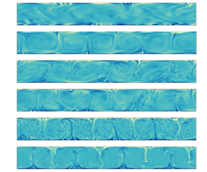
The flow structures are shown in figure 2 by plotting the contours of  $\theta$ at an instant when the flow is statistically stationary. Evidently, no convection rolls are obtained for
 $k_0<4$. Starting from an eight-roll initial state, the GQLA-4 case converges to the six-roll state. Six convection rolls are also obtained for the GQLA-6 case. However, the flow structures are not as explicit as in the GQLA-4 case, and the dynamics of the rolls in GQLA-6 appears to be different from that obtained for GQLA-4. For
 $k_0\ge 8$, eight convection rolls are obtained; for these cases, the converged state is the same as the initial roll state. Contours from the GQLA-128 and DNS cases are qualitatively identical. Among these cases, GQLA-3 belongs to the GQLA regime R1, while the GQLA cases with
 $k_0 \ge 6$ belong to the GQLA regime R3. The GQLA case with
 $k_0=4$ belong to the intermediate GQLA regime, R2.
Contours of instantaneous  $0 \le \theta \le 1$ from the simulations: (a) GQLA-3; (b) GQLA-4; (c) GQLA-6; (d) GQLA-8; (e) GQLA-24; (f) GQLA-64; (g) GQLA-128; (h) DNS. The initial condition for the GQLA simulations is the statistically stationary state in the eight-roll DNS as in (h).

Figure 3 shows the amplitude spectra of  $\theta$ in decibel (dB) units for some chosen cases listed in table 1. The spectra are shown in the (
 $k_x, z/H$) plane, where
 $k_x$ is the integer wavenumber in the horizontal direction; the spectra are plotted up to half-height between the two walls. A logarithmic scale is used for the ordinate to show the spectra clearly both inside the boundary layer and in the bulk. For a reference,
 $\delta _\theta$ is marked for the DNS. The
 $k_0$ is indicated for the GQLA simulations by the vertical dashed lines. Highest amplitude is obtained at
 $k_x=4$ for the DNS at all heights; a second peak is also obtained at
 $k_x=8$. For the GQLA-3 case, deep inside the thermal boundary layer, the peak amplitude is obtained at
 $k_x=3$ which shifts to
 $k_x=4$ close to the edge of the thermal boundary layer. The second peak is obtained at
 $k_x=4$ and at
 $k_x=7$ inside the thermal boundary layer and at the edge of it, respectively, and at
 $k_x=8$ in the bulk for case GQLA-3. For the GQLA-4 case, the highest peaks are obtained at
 $k_x=3$ and 7, inside the thermal boundary layer, and at
 $k_x=7$ and 3 in the bulk, respectively. Wavenumbers associated with the convection rolls
 $k_{roll}=k_x=3$ and 4 correspond to the wavelengths of rolls for the six- and eight-roll states, respectively. As is discussed later, the peak at
 $k_x=4$ corresponds to the peak thermal driving wavelength for most of the cases, except for the GQLA-4 case for which
 $k_x=3$ is the peak thermal driving wavelength. On the other hand, for the GQLA-6 case, the dominant and second most dominant peaks are obtained at
 $k_x=6$ and 3 inside the thermal boundary layer, and at
 $k_x=3$ and 6 in the bulk, respectively. A sudden drop in amplitude of the spectra between the
 $l$- and
 $h$-subspace wavenumbers across
 $k_x=k_0$ and
 $k_x=k_0+1$ is evident for
 $k_0 \ge 24$ at all wall-normal locations. Interestingly, the
 $h$-subspace becomes redundant for case GQLA-64.
Amplitude spectra of  $\theta$ in dB (
 $20\log _{10}({A_\theta }/{A_{\theta, ref}})$) with
 $A_{\theta, ref}=0.01$ unit plotted in the (
 $k_x, z/H$) plane from chosen simulations. The vertical dashed lines show the threshold wavenumber
 $k_0$ for the GQLA. The horizontal dashed line in (
 $a$) marks the thickness of the thermal boundary layer,
 $\delta _\theta$. Corresponding
 $k_0$ regimes are also indicated for the GQLA simulations.

While performing the GQLA of turbulent channel flow based on the streamwise wavenumber, Hernández et al. (Reference Hernández, Yang and Hwang2022a) found that for high  $k_0$,
 $h$-subspace wavenumbers yield the 0 solution. They attributed this property to the convergence of the solution of the linearized
 $h$-subspace equations to the Lyapunov vector associated with the leading Lyapunov exponent of the linear operator. For QLA/GQLA, the leading Lyapunov exponent from the linearized
 $h$-subspace equations must be zero (Farrell & Ioannou Reference Farrell and Ioannou2012). It could be possible that in the current GQLA of the two-dimensional RBC problem for high
 $k_0=64$, the trivial solution is obtained for the
 $h$-subspace wavenumbers because of the convergence of the solution of the linearized
 $h$-subspace wavenumbers to the Lyapunov vector associated with the Lyapunov exponent of the linear operator that approaches 0 with increasing
 $k_0$.
Overall, the amplitudes of the  $l$-subspace wavenumbers from the GQLA simulations clearly overshoot the DNS. The most dominant wavenumbers in the spectra are: the integer wavenumber corresponding to the size of the convection rolls (
 $k_{roll}$), the dominant wavenumber for thermal driving (
 $k_{\hat {Q}}$ which in most
 ${\rm cases}=k_{roll}$ except the GQLA-3 case) and the wavenumber completing the triad with the these two wavenumbers.
In figure 3, for GQLA cases with low  $k_0 \le 24$, a second wavenumber range with non-negligible energy at high wavenumbers for
 $k_x \ge 30$ can be noticed. Figure 4 shows the premultiplied amplitude spectra of
 $\theta$, i.e.
 $({2{\rm \pi} k_x}/{L_x})|\hat {\theta }(k_x, z/H)|$ (here,
 $\hat {\theta }(k_x, z/H)$ is the amplitude of the Fourier mode
 $k_x$ at a distance
 $z/H$ from the lower wall) for the same cases shown in figure 3 in the (
 $k_x, z/H$) plane. A range of scales having non-negligible energy at the edge of the thermal boundary layer and extending up to the bulk region of the flow is evident for the DNS. The result obtained for the current
 $[Ra, Pr]$ combination is in agreement with the DNS results reported by Blass et al. (Reference Blass, Verzicco, Lohse, Stevens and Krug2021) and Berghout, Baars & Krug (Reference Berghout, Baars and Krug2021). This range of energetic scales shrinks for the GQLA. As the thermal boundary layer is thinner for the GQLA simulations, the wall-normal location for this patch shifts closer to the wall for the GQLA. However, the peak for this energetic range is correctly captured by the GQLA at
 $k_x \sim 100$. As this range is also obtained by the GQLA with low
 $k_0 \le 8$ for which this range belongs to the linearized
 $h$-subspace flow, the energy accumulation at these scales may be attributed to the linear instability (the flow is linearly unstable for all scales up to
 $k_x \sim 200$). Additionally, the accumulated energy in GQLA is larger compared to DNS possibly due to the suppressed energy cascade routes due to the omitted triad interactions in GQLA resulting in accumulation of energy extracted by the linear instability for
 $h$-subspace wavenumbers. As is evident from the plot for the GQLA-64 case, the linear instability mechanism by itself is insufficient for sustaining the small scales belonging the
 $h$-subspace for this case.
Premultiplied amplitude spectra of  $\theta$ plotted in the (
 $k_x, z/H$) plane from the GQLA simulations initiated with the statistically stationary solution from DNS. The vertical dashed lines show the threshold wavenumber
 $k_0$ for the GQLA. The horizontal dashed line in (a) marks the thickness of the thermal boundary layer,
 $\delta _\theta$. Corresponding
 $k_0$ regimes are also indicated for the GQLA simulations.

The wall-normal profiles of the mean and turbulent statistics for some chosen eight-roll initial state simulations are shown in figure 5. The profiles for the mean temperature,  $\langle \theta \rangle$, are shown in figure 5(a); to clearly show the thermal boundary layer, a zoomed-in view of the profiles close to the lower wall is shown. Profiles for all the GQLA cases are in reasonably good agreement with the profile from the DNS. For the cases shown in the figure, the steepest profile is obtained for the GQLA-3 case supporting the maximum heat transport between the plates.
Wall-normal profiles of mean flow and Reynolds stresses from the GQLA simulations: (a)  $\langle \theta \rangle$; (b)
 $\langle u'u' \rangle$; (c)
 $\langle w'w' \rangle$; (d)
 $\langle \theta '\theta ' \rangle$. Corresponding
 $k_0$ regimes are also indicated for the GQLA simulations.

The Reynolds stresses due to the horizontal velocity ( $\langle u'u'\rangle$), wall-normal velocity (
 $\langle w'w'\rangle$) and temperature (
 $\langle \theta '\theta '\rangle$) fields are presented in figure 5(b–d), respectively. To clearly show the comparison among the considered cases close to the near-wall peak, in figure 5(d), a zoomed-in view is shown close to the lower plate. Clearly, GQLA overpredicts the Reynolds stresses, specifically for low
 $k_0$. Overpredictions by the GQLA-3 case for
 $\langle w'w'\rangle$ and
 $\langle \theta '\theta '\rangle$ are largest with respect to the DNS. However, GQLA-4 significantly overpredicts
 $\langle u'u'\rangle$ relative to the GQLA-3 case. From both flow structures shown in figure 2 and the statistics presented in figure 5, addition of the important integer wavenumber
 $k_x=4$ in the
 $l$-subspace for GQLA-4 compared with GQLA-3 significantly improves the prediction capability of the GQLA. This is discussed later in more detail. Statistics predicted by the GQLA are remarkably good even for low threshold wavenumbers (
 $k_0\ge 6$). The plots for the Reynolds stresses also show that the convergence of the GQLA to the DNS is non-monotonic.
3.2. Kinetic energy budget
In this section, we discuss the capability of the GQLA in approximating the different terms in the kinetic energy budget equation in (2.17). The calculations for the budget equations in this section and the next are performed once a statistically stationary state is reached in each simulation.
The kinetic energy input to the system is via the thermal driving term,  $\hat {Q}(k_x, z)$, in (2.22). The contours of this quantity are plotted in the
 $(k_x, z/H)$ plane in figure 6 for some chosen cases. Except for the GQLA-3 case, for all other cases, the dominant horizontal wavenumber for the thermal driving (
 $k_{\hat {Q}}$) is the same as the wavenumber associated with the convection-roll wavelength (
 $k_{roll}$) in each simulation; for GQLA-3, no convection roll was obtained (see figure 2). A broad range of wavenumbers contribute towards the thermal driving. For the DNS, for a small range of wavenumbers just outside the thermal boundary layer
 $\hat {Q}<0$ indicating persistent negative correlation between
 $\theta '$ and
 $w'$ there. Interestingly, for the GQLA-3 case, the dominant wavenumber
 $k_{\hat {Q}}=4$ belongs to the
 $h$-subspace. Inside the thermal boundary layer,
 $\hat {Q}<0$ for
 $k_x=3$ for this case. On the other hand, for the GQLA-4 case, the dominant wavenumber is
 $k_{\hat {Q}}=3=k_{roll}$, and not
 $k_x=4$ which belongs to the fully nonlinear
 $l$-subspace. Inside the thermal boundary layer,
 $\hat {Q}<0$ for very large horizontal structures with
 $k_x=2, 3$, and 4 for this case. This also indicates a different underlying dynamics for GQLA-4 compared with DNS. Additionally, in the region between the thermal boundary layer and the bulk, a bulge is obtained in
 $\hat {Q}$ for the energetic high-wavenumber range depicted in figure 4 (
 $200 \ge k_x \ge 30$); this bulge is more significant for GQLA with low
 $k_0 \le 8$. Term
 $\hat {Q}$ suddenly drops off across
 $k_x = k_0$ for the GQLA-24 case; for GQLA-64,
 $\hat {Q} \approx 0$ for the
 $h$-subspace wavenumbers. Despite this sudden dropping off across
 $k_0$, contours for the GQLA cases with
 $k_0 \ge 24$ show good agreement with contours from DNS, including the aforementioned energetic high-wavenumber range with
 $k_x \ge 30$, and also the wavenumber patches where
 $\hat {Q}<0$.
Thermal driving,  $\hat {Q}$, as expressed in (2.22) plotted in the (
 $k_x, z/H$) plane for some chosen cases listed in table 1. The vertical dashed lines show the threshold wavenumber
 $k_0$ for the GQLA simulations. The horizontal dashed line in (a) marks the thickness of the thermal boundary layer,
 $\delta _\theta$, from DNS. Corresponding
 $k_0$ regimes are also indicated for the GQLA simulations.

Contours of the turbulent transport,  $\hat {T}_t$, are plotted in the (
 $k_x, z/H$) plane and shown in figure 7 for the same cases as in figure 6. As previously mentioned, GQLA only directly affects this nonlinear transport term. Clearly, for both the DNS and GQLA, this term is dominant in the bulk, specifically, outside the thermal boundary layer. Also for this term, the dominant wavenumber is
 $k_{roll}$, except for the GQLA-3 case. Parameter
 $\hat {T}_t \ge 0$ for
 $k_{roll}$ for the DNS, except close to the mid-plane between the plates. Nonlinear transport is negative outside the thermal boundary layer for high wavenumbers in figure 7(a) for the DNS, i.e. kinetic energy is transported by small scales away from the bulk; this property is emulated by the GQLA, even for low
 $k_0$. This demonstrates the efficacy of the GQLA in incorporating the scattering mechanism among the
 $h$-subspace wavenumbers. For GQLA cases with
 $k_0 \le 8$, for most of the low wavenumbers
 $k_x \le k_0$,
 $\hat {T}_t < 0$ specifically outside the thermal boundary layer. This indicates, for low
 $k_0$, that large-scale velocity fluctuations also transport kinetic energy away from the bulk, which is in contrast to the results from the DNS and GQLA simulations with
 $k_0 \ge 24$. This also indicates that although the GQLA could capture the convection rolls for
 $k_0 \ge 4$, the dynamics underlying the GQLA simulations with low
 $k_0$ is not the same as that of the DNS. As shown in figure 2, the GQLA simulations with
 $k_0 < 8$ yielded six convection rolls irrespective of the applied initial condition with eight convection rolls and the GQLA with
 $k_0 \ge 8$ in this RBC flow regime.
Turbulent transport,  $\hat {T}_t$, as expressed in (2.18) plotted in the (
 $k_x, z/H$) plane for some chosen cases listed in table 1. The vertical dashed lines show the threshold wavenumber,
 $k_0$, for the GQLA simulations. The horizontal dashed line in (
 $a$) marks the thickness of the thermal boundary layer,
 $\delta _\theta$, from DNS. Corresponding
 $k_0$ regimes are also indicated for the GQLA simulations.

In the results for the kinetic energy budget in this section, both the amplitudes of thermal driving,  $\hat {Q}$, and dissipation,
 $\hat {\varepsilon }$ (not shown here), are higher for the GQLA simulations compared with the DNS. This is mainly because the GQLA dynamics inhibits the cascade of energy by removing some of the triadic interactions entrapping more energy at small wavenumbers, specifically belonging to the
 $l$-subspace. Consequently,
 $\hat {Q}$ is larger at these wavenumbers. In a statistically stationary state, energy input to the system must also be dissipated. As a result, dissipation is also enhanced at low wavenumbers. At increasing levels of the approximation, i.e. for lower
 $k_0$, this effect is more and more pronounced (this can be verified from table 1). Average dissipation,
 $\langle \varepsilon \rangle$, is maximum for
 $k_0=0$, i.e. for the QLA. As a consequence, transport is also enhanced.
Based on  $A_\theta$ plotted in figure 3, and the contours of
 $\hat {Q}$ and
 $\hat {T}_t$ plotted in figures 6 and 7, respectively, the most important wavenumber is
 $k_{\hat {Q}}$ (which is equal to
 $k_{roll}$ for most cases except GQLA-3) which must belong to the
 $l$-subspace wavenumbers for the GQLA to be able to capture the convection rolls. This criterion demarcates the first GQLA regime, R1. In DNS, the convection rolls both extract and dissipate the most energy, as well as transporting the most amount of energy through nonlinear advection. Energy extraction and nonlinear transport are predominantly in the bulk, while the dissipation is highest at the wall where it is concentrated in the low wavenumbers. All these quantities are reasonably predicted by GQLA with
 $k_0 \ge 6$, i.e. in R3. In this GQLA regime,
 $k_0 \ge 2 k_{roll}$, and the fully nonlinear dynamics captured in DNS may be emulated by the restricted nonlinear interactions in GQLA for the
 $k_{roll}$ state under consideration.
3.3. Thermal energy budget
The nonlinear turbulent transport,  $\hat {T}_{\theta, t}$, is the only term in the governing equation for
 $\hat {e}_\theta$ that is directly affected by the GQLA. The contours of
 $\hat {T}_{\theta, t}$ are plotted in the (
 $k_x, z/H$) plane in figure 8 for the same cases as in figures 6 and 7. In contrast to the similar term,
 $\hat {T}_t$ in the kinetic energy budget equation (2.17) which was dominant at the edge of the thermal boundary layer and in the bulk,
 $\hat {T}_{\theta, t} > 0$ throughout the wavenumber range shown, at the edge and inside the thermal boundary layer for all the cases shown. In the bulk, the sign of
 $\hat {T}_t$ is arbitrary. Clearly, turbulent transport of thermal energy is most pronounced at the edge of the thermal boundary layer, and reduces significantly close to the wall and in the bulk, and also at high wavenumbers. The dominant wavenumber in all the cases is the wavenumber
 $k_{roll}$ corresponding to the convection-roll wavelength, except for the GQLA-3 case, for which wavenumbers in the triad
 $k_x=[3, 4, 7]$ are the most active in transporting thermal energy via turbulent fluctuations. For all these cases with
 $k_{roll}$ as the dominant wavenumber,
 $\hat {T}_t(k_x=k_{roll}, z/H) < 0$ for a patch just outside the thermal boundary layer; the convection rolls transport thermal energy away from the bulk and inside the thermal boundary layer. Along with
 $k_{roll}$, high transport is also obtained for the wavenumber corresponding to its harmonic,
 $2k_{roll}$, for the DNS and GQLA cases with
 $k_0 \ge 24$. For the GQLA-4 and GQLA-6 cases, a range of wavenumbers alongside
 $k_{roll}$ is active throughout the thermal boundary layer for
 $k_x \le k_0$. The GQLA cases with
 $k_0 \ge 6$ show a significant drop in
 $|\hat {T}_{\theta, t}|$ across
 $k_0$; for the GQLA-64 case, the
 $h$-subspace wavenumbers are inactive. For all GQLA simulations, the high-wavenumber energetic range at the edge of the thermal boundary layer depicted in figure 4 are also active in transporting thermal energy via turbulent fluctuations. In contrast to the DNS, a wider range of wavenumbers are highly active for all the GQLA simulations.
Nonlinear turbulent transport,  $\hat {T}_{\theta, t}$, as expressed in (2.25) plotted in the (
 $k_x, z/H$) plane for some chosen cases listed in table 1. The vertical dashed lines show the threshold wavenumber,
 $k_0$, for the GQLA simulations. The horizontal dashed line in (a) marks the thickness of the thermal boundary layer,
 $\delta _\theta$, from DNS. Corresponding
 $k_0$ regimes are also indicated for the GQLA simulations.

The inferences drawn for the thermal energy balance are also similar to the thermal driving and dissipation of kinetic energy. The GQLA overpredicts the thermal transport and dissipation (not shown here) compared with the DNS. The overshoot is larger for lower  $k_0$, and largest for
 $k_0=0$, i.e. QLA. Suppression of select nonlinear interactions inhibits cascades that eventually result in dissipation at smaller scales. In contrast, for low
 $k_0$, thermal transport
 $\hat {T}_{\theta, t}$ and dissipation
 $\widehat {\varepsilon _\theta }$ are enhanced at low wavenumbers. As a consequence, heat transport between the two plates is also enhanced;
 $Nu$ increases with a decrease in
 $k_0$ (see table 1).
For both momentum and thermal energy balance, the dominant wavenumber for thermal driving ( $k_{\hat {Q}}$, which in most cases equals
 $k_{roll}$ except for case GQLA-3) dominates transport and dissipation. In addition, for all the GQLA cases except for GQLA-64, a second range of wavenumbers in the
 $h$-subspace (
 $k_x \ge 30$) show enhanced thermal transport and dissipation. A large range of wavenumbers are linearly unstable (
 $k_x < 200$) gaining energy irrespective of the restrictions imposed on nonlinear interactions in the approximation. This is possibly due to the suppression of possible dissipation routes in GQLA, as only the
 $h\to l \to h$ and
 $l \to h \to h$ interactions allow transport of thermal energy to/from higher wavenumbers for dissipation; so, linearly unstable wavenumbers are forced to dissipate more energy rather than cascading the energy down to higher wavenumbers.
3.4. Scale-to-scale energy transfer
To quantify the efficacy of the GQLA in emulating the processes resolved by the fully nonlinear direct simulation, we utilize the scale-to-scale energy transfer functions in (2.31) and (2.32), respectively, for kinetic and thermal energy transfers in all possible triads formed with the horizontal wavenumber,  $k_x$. For any integer threshold wavenumber,
 $k_0$, a phase diagram showing different regions of the plots for
 $T(k_{x, r}, k_{x, g})$ or
 $T_\theta (k_{x, r}, k_{x, g})$ contributed by various triad interactions due to wavenumbers chosen from either the
 $l$- or
 $h$-subspace is shown in figure 9. As in expressions (2.13) and (2.14), there are
 $2^3 = 8$ possible triad interactions among arbitrarily chosen wavenumbers from the two subspaces. The abscissa and ordinate show the receiver wavenumber,
 $k_{x,r}$, and the giver wavenumber,
 $k_{x,g}$, respectively. Note that a linear scale is assumed for the axes. The contour plot should be antisymmetric with respect to
 $k_{x,r} = k_{x,g}$. On either side of this line, the eight possible interactions are marked. The triad interactions dropped in the GQLA are coloured red. Once a spectral decomposition of the flow fields is assumed with respect to a threshold wavenumber,
 $k_0$, this phase diagram will help identify the different triad interactions contributing towards the contours for the transfer functions irrespective of the restrictions imposed on the nonlinear interactions.
Phase diagram of the transfer functions  $T(k_{x, r}, k_{x, g})$ and
 $T_\theta (k_{x, r}, k_{x, g})$ showing different triad interactions involved in scale-to-scale energy transfer. Note that the axes are shown for a linear scale. The triad interactions shown in red are dropped in GQLA.

3.4.1. Kinetic energy transfer
Contours of the transfer function for kinetic energy,  $T(k_{x, r}, k_{x, g})$, are shown in figure 10 for the DNS and some chosen GQLA simulations initiated with the DNS-8 condition. For the GQLA simulations, along both axes,
 $k_{x,r} = k_{x,g} = k_0$ are marked by dashed lines to clearly show the demarcation between the
 $l$- and
 $h$-subspace wavenumbers. For the DNS, on either side of
 $k_{x,r} = k_{x,g}$, contours of
 $T$ indicate two distinct regions of activity in the phase diagram. One of those is along the convection-roll wavenumber,
 $k_{roll} = k_{x, r} = k_{x, g} = 4$, indicating kinetic energy transfer from/to this wavenumber, from all other wavenumbers. Wavenumber
 $k_x = 4$ receives energy from
 $k_x < 8$, and provides energy to
 $k_x \ge 8$, with maximum energy transfer from
 $k_x=4 \to 8$. The other is due to the curved patches on either side of
 $k_{x,r} = k_{x,g}$ (due to logarithmic scales being used for the axes) starting at
 $k_{x,r} = k_{x,g}= 5$ and extending up to very high wavenumbers over more than a decade. This patch clearly identifies a scale-by-scale inverse energy cascade. The triads contributing to this inverse cascade process include the wavenumbers
 $k_x = [k_{x, r}, k_{x, g}, k_{roll}=4 ]$; the convection rolls act as the mediator (Verma Reference Verma2019) in a given triad.
Transfer function  $T(k_{x, r}, k_{x, g})$ showing the scale-to-scale kinetic energy transfer from some chosen cases listed in table 1. Function
 $T(k_{x, r}, k_{x, g}) \ge 0$ for kinetic energy transfer from integer wavenumber
 $k_{x, g} \to$
 $k_{x, r}$ and vice versa. The horizontal and vertical dashed lines correspond to the threshold integer wavenumber,
 $k_0$, for the GQLA simulations. Corresponding
 $k_0$ regimes are also indicated.

With the results from the DNS for comparison, and keeping in mind figure 9 (note that the axes in the current plots use a logarithmic scale), we analyse the results obtained from the GQLA simulations. As the GQLA-3 case does not yield convection rolls, the first energy transfer process to/from  $k_{roll}$ is absent for this case; possibly because of the omission of the
 $h \to l \to l$ and
 $l \to l \to h$ interactions in GQLA, the dominant wavenumber associated with thermal driving,
 $k_x=4$, is unable to directly transfer kinetic energy to potential roll-forming wavenumbers for this case – more on this later. For the same reason, the other process, i.e. the inverse energy cascade obtained in the DNS, is damaged for this case. On the other hand, the GQLA-4 case includes the dominant thermal driving wavenumbers
 $k_x=3$ and 4 within the fully nonlinear
 $l$-subspace, facilitating easy energy transfer from these wavenumbers. The wavenumber
 $k_x=3=k_{roll}$ for this case gains energy from similar wavenumbers, i.e. from
 $k_x < 9$, and provides energy to
 $k_x \ge 10$. The inverse cascade mechanism is also very clear from figure 10(c); the triads involved in the inverse cascade process include
 $k_x = [k_{x, r}, k_{x, g}, k_{roll}=3]$ – the convection rolls acting as the mediator. This energy transfer process is captured by the GQLA even for a low
 $k_0=4$ as in the DNS. Possibly the efficient capturing of this process results in the GQLA-4 case being able to capture the convection rolls. Note, however, that the dominant energy transfer from
 $k_x = k_{roll} \to 2 k_{roll}$ is blocked for this case due to the omission of the
 $l \to l \to h$ (and also
 $h \to l \to l$) triad interaction in GQLA.
The GQLA-6 case on the other hand includes the dominant wavenumber for thermal driving in the fully nonlinear  $l$-subspace. However, it allows for the dominant
 $k_x = k_{roll} \to 2 k_{roll}$ energy transfer route from the rolls. The inverse kinetic energy cascade, although captured, is weak for this case. Similar observations can be made for the GQLA case with
 $k_0 = 24$: the
 $l$-subspace wavenumbers successfully capture both energy transfer processes and sustain the convection rolls. The
 $l$-subspace wavenumbers by themselves are able to emulate the DNS results for the GQLA-64 case. As is also the case for DNS and GQLA-4, for all of these three GQLA simulations (
 $k_0 \ge 6$), the dominant inverse cascade is mediated by the convection rolls. As can be found from figure 9, the inverse cascade process is maintained by the
 $h \to l \to h$ triad interaction especially for low
 $k_0$.
3.4.2. Thermal energy transfer
The transfer function,  $T_\theta$, quantifying the thermal scale-to-scale energy transfer is presented by plotting the contours in the
 $(k_{x, r}, k_{x, g})$ plane in figure 11 for the same cases shown in figure 10. For the DNS, a clear forward cascade process is identifiable by noting the dominant patches either side of and hugging the line
 $k_{x, r}=k_{x, g}$. As was the case for the kinetic energy transfer, the mediator for this process is also
 $k_{roll}=4$ for the DNS. Extraction of
 $T_\theta (k_{x, g}; k_{x, r} = k_{roll}=4$) shows that the maximum thermal energy is transferred from
 $k_x=0 \to 4$ (not included due to the use of logarithmic scale for the axes). Furthermore,
 $3 \le T_\theta (k_{x, g} \le 5; k_{x, r}=4) \ge 0$; however, a large amount of thermal energy is transferred from
 $k_{roll}=4 \to 2k_{roll} = 8$. Except for the dominant thermal energy transfer from
 $k_{x,g}=0 \to k_{x,r}=4$, none of these important processes can be identified for the GQLA-3 case. For the GQLA-4 case, however, the dominant thermal energy transfer is from
 $k_{x,g}=3 \to k_{x,r}=0$, i.e. from the convection rolls to the horizontally invariant length scale. Importantly, instead of the forward cascade, an inverse thermal energy cascade due to the
 $h \to l \to h$ triad interaction, and mediated by
 $k_x=3$, the convection-roll wavenumber for this case, is evident in contrast to the DNS.
Transfer function  $T_\theta (k_{x, r}, k_{x, g})$ showing the scale-to-scale thermal energy transfer from some chosen cases listed in table 1. Function
 $T_\theta (k_{x, r}, k_{x, g}) \ge 0$ for thermal energy transfer from integer wavenumber
 $k_{x, g} \to$
 $k_{x, r}$ and vice versa. The horizontal and vertical dashed lines correspond to the threshold integer wavenumber,
 $k_0$, for the GQLA simulations. Corresponding
 $k_0$ regimes are also indicated.

The results for the GQLA simulations in the R3 regime with  $k_0 \ge 6$ are more akin to the DNS. The wavenumbers associated with the convection rolls for the GQLA cases and the DNS are the same,
 $k_x=4$, in this GQLA regime except for
 $k_0=6$ for which
 $k_{roll}=3$. For all these three cases, the maximum scale-to-scale thermal energy transfer takes place between
 $k_x = 0 \to k_{roll}$. Also for these cases, the forward thermal energy cascade is clearly identifiable, which is mediated by the wavenumber
 $k_x=4$. A milder inverse cascade process alongside the patch indicating the forward cascade is also evident for the GQLA-6 case. In the low-wavenumber end, the cascade process is maintained by the
 $l \to l \to l$ self-interacting triad for the
 $l$-subspace for the GQLA-24 case. For the GQLA-64 case, the whole flow is sustained by the fully nonlinear
 $l$-subspace triad interactions. All GQLA simulations, especially with low
 $k_0$, clearly demonstrate the utility of the inclusion of the
 $h \to l \to h$ triad interaction in capturing the forward thermal energy cascade process. For all three cases,
 $|T_\theta |$ is larger for the GQLA simulations, especially for the
 $l$-subspace wavenumbers, compared with the DNS; the overprediction reduces with increasing
 $k_0$. The correct capture of the energy transfer processes, the cascade processes and dominant energy transfer
 $k_{roll} \to 2k_{roll}$ demarcate the R3 GQLA regime; this is obtained for
 $k_0 \ge 6$ for the DNS-8 initial condition.
3.5. Discussion
The transfer functions (figures 10 and 11) from the direct simulation reveal the involved energy transfer processes. One of the important energy transfer processes is the direct kinetic energy transfer to/from the convection rolls. The maximum amount of thermal energy is first transferred from  $k_x=0 \to k_{\hat {Q}}$, the dominant wavenumber for thermal driving of momentum. For all GQLA cases except GQLA-3 (for which no convection rolls are obtained),
 $k_{roll} = k_{\hat {Q}}$ (see figures 2 and 6–8); the thermal energy in convection rolls then directly drives the momentum field through
 $\hat {Q}$ in (2.17).
The energy transfers to/from  $k_{roll}$ (including thermal energy transfer from wall to
 $k_{roll}$) must be correctly captured for the success of the GQLA, especially at low
 $k_0$. This is because, for low
 $k_0$, as
 $k_x=0$ always belongs to the fully nonlinear
 $l$-subspace in QLA/GQLA, potential convection-roll-forming wavenumbers should also belong to this subspace (in which case,
 $k_{roll} = k_{\hat {Q}}$ condition is satisfied) for efficient transfer of energy to/from the convection rolls via the
 $l \to l \to l$ triad interaction. For this reason, while GQLA-4 yielded convection rolls, GQLA-3 did not. While for GQLA-4,
 $k_{\hat {Q}}=3=k_{roll} < k_0$, for GQLA-3,
 $k_{\hat {Q}}=4 > k_0$ in figure 6. This condition demarcates the boundary between the R1 and R2 GQLA regimes: GQLA can capture convection rolls for
 $k_0 \ge k_{\hat {Q}}$. In addition,
 $h \to l \to l$ and
 $l \to l \to h$ triad interactions are excluded in GQLA hindering transfer of energy to/from the wavenumbers that can potentially yield convection rolls especially for low
 $k_0$ – this is further elaborated in § 4.
The second process is the scale-by-scale energy transfer, an inverse kinetic energy cascade and a forward thermal energy cascade in DNS. This process is also mediated by the convection rolls. In GQLA, these processes are captured by the  $h \to l \to h$ triad interactions by the
 $h$-subspace wavenumbers. The involved triads include the donor and receiver wavenumbers separated by
 $k_{roll}$. This process was found to be very important for GQLA simulations with low
 $k_0 <6$, i.e. in the R1 and R2 regimes of GQLA. For example, this process is strong and contributes significantly towards sustenance of the convection rolls in case GQLA-4. Inverse thermal and kinetic energy cascades are obtained for both GQLA-3 (in the R1 regime) and GQLA-4 (in the R2 regime).
Based on the transfer functions calculated for the DNS, the largest amount of energy is always transferred from  $k_{roll} \to 2k_{roll}$. In the case
 $k_0 \ge 2k_{roll}$, such as for
 $k_0 \ge 6$, captured GQLA dynamics is similar to the fully nonlinear dynamics. This condition demarcates the third and final R3 GQLA regime. In this regime, dominant energy transfer processes, namely the energy transfer to/from the convection rolls, and the inverse kinetic energy cascade process and the forward thermal energy cascade process are faithfully captured by GQLA, and as a consequence is able to replicate the fully nonlinear dynamics. Specifically, the cascade processes are captured by the
 $h \to l \to h$ triad interaction for the
 $h$-subspace wavenumbers, especially for low
 $k_0$.
In the intermediate GQLA regime, i.e. R2, for  $2k_{roll} > k_0 \ge k_{\hat {Q}}$,
 $k_{roll}=3$ always belongs to the
 $l$-subspace for GQLA simulations with
 $k_0 < 6$. For GQLA-4, the wavenumber
 $k_x = 8 > k_0$ (corresponding to
 $2k_{roll}$ for the eight-roll state) which cannot receive any energy because of the omission of the
 $h \to l \to l$ and
 $l \to l \to h$ triad interactions in GQLA. However,
 $2k_{roll} = 6$ (for the six-roll state) can receive energy for GQLA simulations with
 $6 > k_0 \ge 4$; in this regime,
 $2k_{roll} > k_0 \ge k_{\hat {Q}}$ is thus satisfied and the eight-roll state cannot be yielded. The nonlinear dynamics captured in this GQLA regime is different from that of the fully nonlinear DNS. For example, plots both for
 $T(k_x, z/H)$ in figure 10(c) and for
 $T_\theta (k_x, z/H)$ in figure 11(c) show inverse cascade processes for kinetic and thermal energies for the
 $h$-subspace wavenumbers for the GQLA-4 case. However, for DNS, only the scale-to-scale kinetic energy transfer process involves an inverse cascade process, while for the thermal energy, a forward cascade process is obtained. Although we note that the transfer functions are volume-averaged results as in (2.31) and (2.32), in figure 6, the thermal driving of momentum inside the thermal boundary layer for the GQLA-4 case at the convection-roll wavenumber
 $\hat {Q}(k_x=k_{roll}=3)< 0$ in contrast to the DNS. From the contour plots of
 $\theta '$ and
 $w'$, these correspond to regions of plume ejection at the two walls.
The results presented herein, especially the kinetic and thermal energy balance presented in figures 6–8, and the scale-to-scale energy transfer functions in figures 10 and 11 provide some reasoning behind GQLA's non-monotonic convergence with DNS for RBC: based on the choice of  $k_0$, certain processes may be hindered or facilitated that dictate the formation and sustenance of the convection rolls, cascading (and consequently dissipation), etc. For example, the dominant thermal energy transfer to/from
 $k_x=k_{roll}$ may be hindered based on the choice of
 $k_0$, or dominant energy transfer from
 $k_{roll} \to 2 k_{roll}$ as in DNS may be hindered or entirely removed in GQLA for low
 $k_0 < 6$.
4. Nonlinear scale interaction studies
With the decomposition of a flow field into  $l$- and
 $h$-subspace components, the GQLA framework may be utilized as an intrusive tool to study the influence of different nonlinear triad interactions arising in the fully nonlinear equations. Instead of dropping the terms as in GQLA, target interaction terms may be included/dropped to study the influence of the chosen interactions on the approximated nonlinear dynamics. In this section, we use this methodology to study the influence of some of the nonlinear triad interactions in (2.13) and (2.14). One should be careful, however, in choosing the interactions to be suppressed. For example, in our work, we retain/drop interactions such that for a given triad, both the receiver and giver wavenumbers are able to exchange energy with each other, i.e. for a triad
 $k_x = [\alpha, \beta, \gamma ]$, energy transfer routes
 $\alpha \to \beta \to \gamma$ and
 $\gamma \to \beta \to \alpha$ are both included/omitted in the experiment.
The intrusive simulation performed herein is intended to understand the influence of the omitted triad interactions in GQLA-3 (in general, for  $k_0 < k_{\hat {Q}}$) that are responsible for its inability to capture the convection rolls for the DNS-8 initial condition. For the GQLA-3 case initiated with the DNS-8 condition,
 $k_{\hat {Q}} = k_x = 4 > 3 = k_0$. Here, we study if the inclusion of the
 $h \to l \to l$ and
 $l \to l \to h$ interactions yields the convection rolls in a trial simulation with
 $k_0=3$ (convection rolls were only obtained for
 $k_0 \ge 4$). We also consider an additional GQLA-3 calculation for which the initial condition is the same as DNS (see the Appendix for all GQLA simulations initiated with this initial condition). Comparison of results from this simulation with T-3 and GQLA-3 cases initiated with the DNS-8 condition illustrates the influence of the initial condition. We note that the conclusions drawn are dependent on the choice of
 $k_0$; however, we also emphasize that the inferences are valid below the chosen limit of
 $k_0$.
Table 2 tabulates triad interactions included/discarded in the intrusive calculation and compared with the GQLA simulation. A direct simulation includes all the eight triad interactions listed. In case T-3, in addition to the four triadic interactions included in the standard GQLA, we also include the  $hll$ (
 $h \to l \to l$) and
 $llh$ (
 $l \to l \to h$) interactions for the
 $l$- and
 $h$-subspace wavenumbers, respectively. The different initial conditions for these simulations are also listed.
Triad interactions included/discarded in the additional simulations. Here,  $\alpha \beta \gamma$ indicates the
 $\alpha \to \beta \to \gamma$ triad interaction.

4.1. Flow visualizations, statistics and spectra
Contours of  $\theta$ showing the flow structures are shown in figure 12 for the intrusive calculation. The flow structures from the T-3 simulation are somewhat similar to those of the GQLA-4 case shown in figure 2(c) – six large-scale convection rolls are obtained along with other large-scale fluctuations. The inclusion of the two additional interactions indeed results in the formation of rolls for low
 $k_0=3$, and the resultant approximation is akin to GQLA with
 $k_0=4$. The obtained state is different from the initial roll state, and is akin to the R2 GQLA regime (
 $2k_{roll} > k_0 \ge k_{\hat {Q}}$). On the other hand, the GQLA-3 calculation with the random initial condition also yields six convection rolls in figure 18(b) (see the Appendix), and the dynamics of the convections rolls is similar to that obtained for GQLA-4 with the DNS-8 initial condition.
Contours of instantaneous  $0 \le \theta \le 1$ from the intrusive calculation listed in table 2: case T-3 initiated with the DNS-8 condition.

Table 3 tabulates  $\delta _\theta$,
 $Nu$,
 $\langle \varepsilon \rangle$ and
 $r_f$ – the number of convection rolls yielded at a statistically stationary state for these additional calculations. Parameter
 $\delta _\theta$ obtained for the trial approximation T-3 is larger than for the baseline GQLA-3 case. Additionally, inclusion of the two additional interactions significantly alters
 $Nu$ and
 $\langle \varepsilon \rangle$; both these quantities reduce compared with the baseline GQLA-3 simulation with the DNS-8 initial condition and are closer to the results obtained from DNS (see table 1). It must be noted that, because of
 $k_0=3$ being low, only a handful of additional triads (six additional triads for each of the two interactions) are included in the approximation for the T-3 case. Interestingly, in spite of using the same GQLA with the same
 $k_0$, GQLA-3 with the random initial condition yields
 $Nu$ and
 $\langle \varepsilon \rangle$ closer to the DNS compared with both the T-3 case and the baseline GQLA-3 initiated with the DNS-8 condition highlighting the influence of the initial condition of the simulations in this RBC regime (Wang et al. Reference Wang, Verzicco, Lohse and Shishkina2020).
Details of the additional calculations.

Wall-normal profiles of  $\langle \theta \rangle$, and the Reynolds stresses corresponding to
 $u$- and
 $w$-components and
 $\theta$ are shown for case T-3 along with the baseline GQLA-3 case both initiated with the DNS-8 condition, and compared with GQLA-3 initiated with the random condition in figure 13. Zoomed-in views are presented for
 $\langle \theta \rangle$ and
 $\langle \theta '\theta ' \rangle$ profiles only close to the lower wall in figures 13(a) and 13(d), respectively. The
 $\langle \theta \rangle$ profile is steeper for the baseline GQLA-3 case. Both T-3 and GQLA-3 with random initial condition cases overshoot and undershoot
 $\langle \theta \rangle = 0.5$ in the bulk, respectively, for
 $z/H \le 0.5$ and
 $z/H \ge 0.5$. Both these cases yield much better predictions for the
 $u$- and
 $w$-components of the Reynolds stress compared with its baseline GQLA-3 in figures 13(b) and 13(c). Also, the Reynolds stress due to
 $\theta '$ close to the lower wall in figure 13(d) shows that both these cases provide much better predictions compared with the baseline GQLA-3 initiated with the DNS-8 condition. The overall predictions are slightly better for the T-3 case compared with GQLA-3 with random initial condition possibly because of the inclusion of the additional triads for the T-3 case.
Wall-normal profiles of mean flow and Reynolds stresses from the additional calculations compared with the corresponding baseline GQLA simulations with different initial conditions: (a)  $\langle \theta \rangle$; (b)
 $\langle u'u' \rangle$; (c)
 $\langle w'w' \rangle$; (d)
 $\langle \theta '\theta ' \rangle$.

Despite the use of a biased initial condition, additional triadic interactions included for the T-3 case enables it to transition from the initial eight-roll state dominated by  $k_x=4$ to the six-roll state dominated by
 $k_x=3$. This is probably possible due to the included
 $h \to l \to l$ triad interactions which allows it to drain energy from the
 $k_x=4 \to 3$ which is not included for the baseline GQLA-3 case also initiated with the biased DNS-8 condition. The GQLA-3 case initiated with the random condition is not influenced by this bias. Because the statistically stationary states yielded for the T-3 case and the GQLA-3 case initiated with the random condition are very similar, in the rest of our discussion in this section we use T-3 as the representative case for comparison between the GQLA and trial approximation.
The amplitude spectra of  $\theta$ and
 $A_\theta$ and the premultiplied spectra are shown in figure 14 for the T-3 case in the (
 $k_x, z/H$) plane. The T-3 case yields a peak corresponding to the six-roll state obtained for this case, i.e. for
 $k_{roll}=k_x=3$ at all
 $z/H$ locations shown; a second peak is also obtained for
 $k_x=6$ close to the wall, which becomes the primary peak at the outer edge of the thermal boundary layer. A second range of wavenumbers accumulating high energy is also obtained in the premultiplied spectra for
 $k_x \ge 30$ which peaks close to
 $k_x \sim 150$.
Spectra of  $\theta$: (a)
 $A_\theta$ in dB (
 $20\log _{10}({A_\theta }/{A_{\theta, ref}})$) unit with
 $A_{\theta, ref}=0.01$; (b) premultiplied spectra plotted in the (
 $k_x, z/H$) plane from the T-3 case. The vertical dashed lines mark the threshold wavenumber,
 $k_0$.

4.2. Kinetic and thermal energy budget
The thermal driving of the momentum due to the  $\theta$ field,
 $\hat {Q}$, is plotted in the (
 $k_x, z/H$) plane for the T-3 case in figure 15(a). The dominant wavenumber for
 $\hat {Q}$,
 $k_{\hat {Q}}=k_x=3$ for case T-3 – the wavenumber associated with the convection rolls. Driving
 $\hat {Q} < 0$ at the dominant wavenumber,
 $k_x=3$ for
 $z/H \le 0.03$, within the thermal boundary layer. This property is consistent with the GQLA simulations with
 $6 > k_0 \ge 4$ for the DNS-8 condition, i.e. in the R2 regime, for which six convection rolls were also obtained (e.g. plot for
 $\hat {Q}$ for the GQLA-4 case in figure 6c). The second dominant wavenumber corresponds to
 $k_x=6$. At this wavenumber
 $\hat {Q} \ge 0$ within the thermal boundary layer, and
 $\hat {Q} < 0$ outside the thermal boundary layer, in a considerable region in the bulk,
 $0.35 \ge z/H \ge 0.08$.
(a) Thermal driving,  $\hat {Q}$, and (b) nonlinear turbulent transport of momentum,
 $\hat {T}_t$, as expressed in (2.22) plotted in the (
 $k_x, z/H$) plane for the T-3 case. The vertical dashed lines show the threshold wavenumber,
 $k_0$.

Momentum/heat transported by the flow, denoted by  $\hat {T}_t$ and
 $\hat {T}_{\theta, t}$ in the kinetic/thermal energy budget equations in (2.17) and (2.24), respectively, is directly affected by the case-specific approximation. The contours for these quantities are shown in figures 15(b) and 16 for the T-3 case in the (
 $k_x, z/H$) plane. Momentum transport is mainly in the bulk, while the thermal transport mainly takes place at the edge of the thermal boundary layer. The results are significantly improved compared with the baseline GQLA-3 case. Compared with the GQLA-3 case with DNS-8 condition in figures 7(b) and 8(b), the main noticeable difference is that the transport is dominated by the wavenumber corresponding to the convection rolls in this case, i.e.
 $k_{roll}=3$. Similar to the GQLA-3 case, the amplitudes of these quantities are overpredicted for this case compared with DNS at low wavenumbers.
Nonlinear turbulent transport of thermal energy,  $\hat {T}_{\theta, t}$, plotted in the (
 $k_x, z/H$) plane for the T-3 case. The vertical dashed line marks the threshold wavenumber,
 $k_0$.

Although not shown herein, the spectral distributions of kinetic energy dissipation,  $\hat {\varepsilon }$, and thermal energy dissipation,
 $\hat {\varepsilon }_\theta$, also show similar properties. Both
 $\hat {\varepsilon }$ and
 $\hat {\varepsilon }_\theta$ are largest at the wall for the wavenumber corresponding to the convection roll (
 $k_x=3$) for the T-3 case followed by the second peak at
 $k_x=6$. Both
 $\hat {\varepsilon }$ and
 $\hat {\varepsilon }_\theta$ slowly drop up to
 $k_x \sim 30$;
 $\hat {\varepsilon }$ plateaus up to
 $k_x \sim 100$ followed by sharp drop-off. On the other hand,
 $\hat {\varepsilon }_\theta$ sharply rises again for
 $k_x > 30$ inside the thermal boundary layer; a secondary peak is obtained at
 $k_x\sim 110$ followed by drop-off.
4.3. Scale-to-scale energy transfer
The scale-to-scale kinetic energy transfer is presented in figure 17(a) by plotting the transfer function,  $T(k_{x, r}, k_{x, g})$, for the T-3 case. Function
 $T(8 \le k_{x, r} \le 14, k_{x, g}=3, ) > 0$, implying that kinetic energy is transferred from the convection rolls with
 $k_{x, g}=3 \to 8 \le k_{x, r} \le 14$; the largest amount of energy is transferred to
 $k_{x, r}=9=3k_{roll}$ which belongs to the
 $h$-subspace. Scales similar to the convection rolls, i.e.
 $k_{x, g} < 5$, provide energy to the convection rolls
 $k_{x, r}=k_{roll}=3$. Part of these direct kinetic energy transfers to/from the convection rolls (among
 $3 \le k_x \le 6$) is facilitated by the inclusion of the two additional triad interactions (
 $hll$ and
 $llh$) for this case. These interactions are therefore paramount for allowing the transition from the initial eight-roll state to the statistically stationary six-roll state for this case. The small scales also transfer energy to the rolls. The scale-by-scale inverse energy cascade at high wavenumbers obtained for the DNS case in figure 10(a) is captured for this case by the
 $h$-subspace wavenumbers up to
 $k_x \sim 10$, beyond which a forward cascade is obtained. The amplitude of the transfer function is also in good agreement with the DNS. Clearly, the results for this case are much improved compared with the baseline GQLA-3 case.
Transfer functions: (a)  $T(k_{x, r}, k_{x, g})$ showing the scale-to-scale kinetic energy transfer and (b)
 $T_\theta (k_{x, r}, k_{x, g})$ showing the scale-to-scale thermal energy transfer from the T-3 simulation. The horizontal and vertical dashed lines correspond to the threshold wavenumber,
 $k_0$.

Contours of instantaneous  $0 \le \theta \le 1$ from the GQLA simulations initiated with the random condition: (a) GQLA-0; (b) GQLA-3; (c) GQLA-4; (d) GQLA-6; (e) GQLA-8; (f) GQLA-12; (g) GQLA-16; (h) GQLA-24.

The transfer function for the thermal scale-to-scale energy transfer,  $T_\theta (k_{x, r}, k_{x, g})$, for the T-3 case is shown in figure 17(b). Inclusion of the
 $hll$ and
 $llh$ triad interactions facilitates the transfer of thermal energy to/from
 $k_{roll} = 3$, which gains most of its energy directly via thermal driving; the highest thermal energy transfer takes place from
 $k_{x, g}=3 \to k_{x, r}=6=2k_{roll}$. This route is absent for the baseline GQLA-3 in figure 11(b). The forward thermal energy cascade for the
 $h$-subspace wavenumbers is captured in the T-3 case, unlike in GQLA-3. This emphasizes the importance of resolving both the energy transfer processes in approximations for successful capturing of the convection rolls.
Finally, it should be noted that the motivation behind this section is to explore whether the GQLA model can be improved by testing specific nonlinear interactions. While energy conservation is certainly an important aspect, our primary aim here was to identify potential improvements in the model's performance. By isolating specific interactions, we sought to determine whether such refinements could lead to a more accurate representation of the system. However, we recognize the importance of energy conservation and plan to investigate this aspect more thoroughly in future studies. A detailed examination of energy dynamics will be critical for further validating and refining the GQLA model, and we are committed to addressing this in our ongoing research.
5. Conclusions
In this work, the GQLA is applied to the two-dimensional planar RBC problem. Application of a spectral decomposition with respect to a threshold wavenumber,  $k_0$, to quadratic nonlinear terms such as in the OBEs results in eight terms representing all the nonlinear triad interactions between the large-scale (l) and small-scale (h) flows, as in (2.13) and (2.14). In GQLA, some triad interactions are dropped; however, it retains the
 $h \to l \to h$ scattering that allows for the small-scale flow to interact among itself mediated by the large-scale flow (Marston et al. Reference Marston, Chini and Tobias2016), which improves its prediction capability compared with the QLA. The current work explores the GQLA's ability to capture the scale-by-scale energy transfer processes in a RBC flow using its restricted nonlinearity.
For the flow considered herein,  $[Ra, Pr ]= [10^8, 10 ]$, in a computational domain with an aspect ratio of
 $8$, at least two decades of wavenumbers (up to integer wavenumber,
 $k_x \sim 200$) are linearly unstable, and these scales extract energy irrespective of the GQLA, as shown in the spectra (figures 3 and 4). Two initial conditions are tested as the flow is sensitive to initial conditions (Wang et al. Reference Wang, Verzicco, Lohse and Shishkina2020). In one, the statistically stationary state with eight convection rolls from the direct simulation was used as the initial condition (DNS-8) for the GQLA simulations. In the other, random perturbations are superimposed on a linear conductive temperature profile with
 $\boldsymbol {u}=0$ (Appendix). Irrespective of the initial conditions, three approximation regimes are identified for the GQLA based on the threshold integer wavenumber (
 $k_0$) segregating the large- (l) and small-scale (h) flow (see figures 2 and 18). In the first low-
 $k_0$ regime, R1, the GQLA is unable to capture the convection rolls for
 $k_0 < k_{\hat {Q}}$, where
 $k_{\hat {Q}}$ is the dominant wavenumber for thermal driving of the flow (see figure 6). The limit demarcating this regime for the present flow is
 $k_0 < 4$ for the DNS-8 initial condition (see table 1). In the third
 $k_0$ regime for
 $k_0 \ge 2k_{roll}$, called R3 herein, the GQLA can replicate the fully nonlinear dynamics (see figures 10 and 11) and can capture the flow's dependence on the initial roll state. The R3 GQLA regime for the present flow is obtained for
 $k_0 \ge 2k_{roll} = 6$ for both initial conditions. In the intermediate GQLA regime, called R2 herein, for
 $2k_{roll} > k_0 \ge k_{\hat {Q}}$, although the GQLA can capture the convection rolls, the nonlinear dynamics captured is different from that of the fully nonlinear flow. In this limit with
 $6 > k_0 \ge 4$, GQLA always yielded six convection rolls as the statistically stationary state for the current flow. This RBC flow yields multiple convection-roll states based on initial conditions of the simulations. Both eight-roll and six-roll states have been reported by Wang et al. (Reference Wang, Verzicco, Lohse and Shishkina2020). Whether the different GQLA dynamics in the R2 and R3 regimes can explain the existence of the multiple states remains an open question.
The R1 regime with  $k_0 < k_{\hat {Q}}$ is characterized by large
 $Nu$ – heat transport is maximum for QLA, i.e. GQLA with
 $k_0=0$. In the R2 regime, as the convection rolls are captured,
 $k_{roll}=k_{\hat {Q}}$, and
 $Nu$ drops and tends towards
 $Nu$ obtained from DNS. Additionally, the GQLA can capture the energy cascade processes mediated by the convection rolls with some success. These processes are maintained by the
 $h$-subspace wavenumbers in this GQLA regime and may be attributed to the
 $h \to l \to h$ triad interaction (compare figures 9, 10 and 11). However, in this low-
 $k_0$ regime, due to the exclusion of the
 $h \to l \to l$ and
 $l \to l \to h$ triad interactions in GQLA, the dominant energy transfer from
 $k_{roll} \to 2k_{roll}$ is blocked. In the final GQLA regime (R3) with
 $k_0 \ge 2k_{roll}$, the energy transfers to/from the convection rolls are also effectively captured. Based on the choice of
 $k_0$ in this regime, the energy cascade processes may be entirely captured by the
 $l$-subspace wavenumbers via the
 $l \to l \to l$ interaction (for high
 $k_0$) or captured in portions by both the
 $l$- and
 $h$-subspace wavenumbers (low to moderate
 $k_0$) via the
 $l \to l \to l$ and
 $h \to l \to h$ interactions, respectively.
Turbulent statistics shown in figure 5 significantly improve even for low  $k_0$ in the R3 GQLA regime. However, in all three GQLA regimes, the spectra and terms contributing to balancing the kinetic and thermal energy budgets in (2.17) and (2.24) are overpredicted for the
 $l$-subspace wavenumbers (e.g. figures 3 and 6–8). In these figures, a high-wavenumber range (
 $200 > k_x \ge 30$) gains energy via linear instability of these scales in all GQLA simulations and is appreciably active. Overshoot in both the
 $l$-subspace wavenumbers and the energetic high-wavenumber range may be attributed to the suppression of select nonlinear interactions, which inhibits cascades that eventually results in dissipation. For the present flow,
 $h$-subspace wavenumbers cannot sustain themselves and become redundant for GQLA with high
 $k_0 \ge 64$.
Additional calculation was performed utilizing the framework underlying the GQLA of decomposing a flow field into large- and small-scale motions and altering select nonlinear triad interactions. The inclusion of the  $h \to l \to l$ and
 $l \to l \to h$ triad interactions with respect to the baseline GQLA with
 $k_0=3$ in this intrusive calculation was intended to understand the GQLA's inability to capture the convection rolls in the first
 $k_0$ regime for the current flow. The initial condition was the statistically stationary eight-roll state obtained in DNS. In this experimental case T-3, six convection rolls were obtained once a statistically stationary state was reached akin to the R2 GQLA regime, establishing the argument that the exclusion of the
 $h \to l \to l$ and
 $l \to l \to h$ triad interactions in GQLA hinders nonlinear transitions in state in the R1 regime. Obtained flow statistics significantly improved for this case compared with the baseline GQLA-3 with the DNS-8 initial condition. Apart from
 $k_{roll} = 3$, high energy was also obtained at
 $2k_{roll}$ due to the additional interactions. The transfer functions plotted in figure 17 show that this case effectively capture both energy transfer processes: the dominant energy transfer to/from the convection rolls, and the scale-by-scale inverse kinetic energy cascade, and forward thermal energy cascade.
Funding
We gratefully acknowledge financial support from the Max Planck Society, the German Research Foundation (DFG) from grants 521319293, 540422505 and 550262949 and the Daimler and Benz foundation. We also thank the HPC systems of Max Planck Computing and Data Facility (MPCDF) for the allocation of computational time.
Declaration of interests
The authors report no conflict of interest.
Data availability statement
The data that support the findings of this study are available upon reasonable request.
Appendix. Initial condition dependence
Wang et al. (Reference Wang, Verzicco, Lohse and Shishkina2020) demonstrated that the RBC flow for  $[Ra, Pr]=[10^8, 10]$ used in the current study exhibits multiple convection roll states depending on the initial condition of the simulations. They obtained eight or six convection rolls for aspect ratio
 $\varGamma = 8$. In the results presented so far, an eight-roll-state initial condition (DNS-8) obtained from the statistically converged flow field from DNS was used for the GQLA simulations. In the results presented herein we use a ‘random’ initial condition as was used for the DNS: a
 $\theta$ field consisting of random perturbations superimposed on the linear conductive profile along with
 $\boldsymbol {u} = 0$. So, we call this initial condition ‘random’. Here we show that the GQLA regimes obtained for the random initial condition are consistent with those obtained for the DNS-8 initial condition.
Table 4 tabulates the boundary-layer thickness,  $\delta _\theta$, Nusselt number,
 $Nu$, and time- and volume-averaged momentum dissipation,
 $\langle \varepsilon \rangle$. The number of convection rolls (
 $r_f$) yielded in the simulations at statistically stationary states is also listed. The flow structures for these GQLA simulations are shown by plotting the instantaneous contours of
 $\theta$ in figure 18. Except for GQLA-3 and GQLA-8 cases, all other cases show good agreement with the same quantities reported for the DNS-8 condition in table 1 and figure 2. Interestingly, GQLA-3 yields six convection rolls unlike for the DNS-8 initial condition for which no rolls were obtained. Capturing the convection rolls results in a significantly reduced
 $Nu$ and
 $\langle \varepsilon \rangle$, and a slightly larger
 $\delta _\theta$ for the random condition compared with the DNS-8 condition for GQLA-3. The dominant wavenumber for thermal driving for this case is
 $k_{\hat {Q}}=3$ for the random condition (not shown here) compared with
 $k_{\hat {Q}}=4$ for the DNS-8 condition. Clearly, the different initial conditions are the primary reason for the large differences noted for the two GQLA-3 cases compared. The GQLA-3 case initiated with the random condition is not influenced by the bias inherent in the DNS-8 initial condition, and converges to a roll state satisfying
 $k_0 \ge k_{\hat {Q}}$, i.e. in the R2 regime of GQLA.
Details of GQLA simulations initiated with the random condition:  $\delta _\theta$ represents the thermal boundary-layer thickness obtained using the slope method and
 $r_f$ indicates the number of convection rolls yielded at a statistically stationary state.

On the other hand, for GQLA-8, six (eight) convection rolls are obtained for the random (DNS-8) initial condition. This results in a thinner thermal boundary layer and a reduced  $Nu$ for the random initial condition compared with the DNS-8 initial condition. Wavenumber
 $k_0 \ge 6$ is representative of the R3 GQLA regime (because
 $k_0=6 \ge 2k_{roll}=6$ for this case). In contrast, GQLA-24 for the random initial condition yields eight convection rolls as in the DNS. Interestingly, GQLA-12 and GQLA-16 yield eight and six convection rolls, respectively, again highlighting the non-monotonic nature of GQLA's convergence to DNS with increasing
 $k_0$, and also the flow's sensitivity to initial conditions. Clearly, all these three cases also belong to the R3 regime of GQLA.
The flow statistics are shown for the GQLA cases initiated with the random condition in figure 19. Comparing with figure 5, GQLA-4 yields similar statistics irrespective of the initial condition indicating that this belongs to the same approximation regime, R2. The GQLA-3 case (also belonging to the R2 GQLA regime) yields consistent statistics when compared with GQLA-4 for the random condition in contrast to the DNS-8 condition. Excellent agreement with DNS for one-dimensional statistics is obtained for GQLA-6, GQLA-8, GQLA-16 and GQLA-24. The flow statistics diverge with respect to the DNS for GQLA-12 considering that this case also yields eight convection rolls for the random initial condition. Clearly, GQLA's convergence with DNS is non-monotonic with increase in  $k_0$ for both the initial conditions used in this work. Overall, in the absence of the initial condition bias for the random initial condition, statistics obtained from GQLA are more consistent compared with the DNS-8 condition for this flow.
Wall-normal profiles of mean flow and Reynolds stresses from the GQLA simulations initiated with the random condition: (a)  $\langle \theta \rangle$; (b)
 $\langle u'u' \rangle$; (c)
 $\langle w'w' \rangle$; (d)
 $\langle \theta '\theta ' \rangle$. Corresponding GQLA
 $k_0$ regimes are also indicated.

For a random initial condition, the GQLA yields six convection rolls for  $k_0 \le 8$. On the other hand, for the DNS-8 initial condition, GQLA yields six convection rolls in the R2 regime (
 $k_0 < 2 k_{roll} =6$), and depending on the initial roll state, yields eight convection rolls for
 $k_0 \ge 8$ in the R3 regime of GQLA. Whether the capturing of the six convection rolls for the DNS-8 condition by the GQLA in the R2 regime or in the R3 regime for
 $k_0=6$ (and also for
 $k_0=8$ for the random condition) is related to the existence of the multiple states remains an open question. Furthermore, the ability of the GQLA to capture both six and eight convection rolls depending on the approximation regime (restriction in nonlinearity) indicates that nonlinear triadic scale interactions could play an important role in the emergence of the multiple states.


 Open access

