


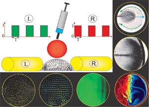

1. Introduction
With the advent of miniaturization, droplet-based microfluidics, which is ubiquitous in protein crystallization, biosensor, immunoassays, DNA-replication, cell-based assays, biomolecular extractions -- to name a few -- has emerged as an effective approach for precise manipulation of a discrete volume of fluid samples and analytes in recent years (Tice et al. Reference Tice, Song, Lyon and Ismagilov2003; Mary, Studer & Tabeling Reference Mary, Studer and Tabeling2008; Berry, Alarid & Beebe Reference Berry, Alarid and Beebe2011; Zhang et al. Reference Zhang, Park, Liu, Tsuan, Yang and Wang2011; Bogojevic et al. Reference Bogojevic, Chamberlain, Barbulovic-Nad and Wheeler2012; White et al. Reference White, Heyries, Doolin, VanInsberghe and Hansen2013; Shamsi et al. Reference Shamsi, Choi, Ng and Wheeler2014). One promising application of droplet-based microfluidics finds huge relevance to the micromixing technology, typically used in on-chip biochemical and biological analysis. The paradigm of droplet-based micromixing can be classified into two different types, namely open surface and closed surface micromixing. Open surface droplet-based micromixing offers a few advantages over the closed surface microfluidic environment, such as simple fabrication, free from any blockage such as bubble clogging (Greenspan Reference Greenspan1978; Smith Reference Smith1995; Long et al. Reference Long, Shetty, Solomon and Larson2009; Tam et al. Reference Tam, von Arnim, Mckinley and Hosoi2009; Pournaderi & Pishevar Reference Pournaderi and Pishevar2014; Lin et al. Reference Lin, Li, Lin, Shu, Wang, Zhang, Yang, Liu and Xu2017). It may be mentioned here that droplet-based mixing in the open surface microfluidic platform can be accomplished by using two approaches viz., the passive approach and the active approach. The passive approach entirely depends on the molecular diffusion between the phases to be mixed and can be tuned by altering the surface morphology (for example, a patterned wettability controlled surface) towards achieving the desired controllability of the mixing (Xing, Harake & Pan Reference Xing, Harake and Pan2011; de Groot et al. Reference de Groot, Veserat, Berthier, Beebe and Theberge2016). While the active approach, which is more prevalent due to its reconfigurable flexibility, primarily relies on external force fields such as an electric field, magnetic field, acoustic waves and light energy for manoeuvring the flow velocities inside the droplet domain (Shang, Cheng & Zhao Reference Shang, Cheng and Zhao2017; Meng & Colonius Reference Meng and Colonius2018; Singh, Das & Das Reference Singh, Das and Das2018; Behera, Mandal & Chakraborty Reference Behera, Mandal and Chakraborty2019; Grassia Reference Grassia2019).
Of all these active approaches, utilization of the magnetic field has evolved as a promising technology in the paradigm of droplet-based mixing in microfluidic platforms, attributed primarily to its inherent advantageous features. A few of such notable features include biocompatibility, ease of incorporation, low cost, less invasive, no induction heating, precise manipulation of the contact line and many more (Nguyen Reference Nguyen2012; Huang et al. Reference Huang, Li, Yang, Li, Li, Yang and Xu2017; Zhang & Nguyen Reference Zhang and Nguyen2017; Liu et al. Reference Liu, Li, Li, Yang, Li, Lu, Li and Xu2018). It is worth mentioning here that researchers have exploited the flexibility of magnetic field driven flow manipulation in the open surface microfluidic framework to achieve controlled mixing in small fluid volumes (Biswal & Gast Reference Biswal and Gast2004; Franke et al. Reference Franke, Schmid, Weitz and Wixforth2009; Lee et al. Reference Lee, van Noort, Lee, Zhang and Park2009; Martin, Shea-Rohwer & Solis Reference Martin, Shea-Rohwer and Solis2009; Roy et al. Reference Roy, Sinha, Chakraborty, Ganguly and Puri2009; Sing et al. Reference Sing, Schmid, Schneider, Franke and Alexander-Katz2010; Vilfan et al. Reference Vilfan, Potočnik, Kavčič, Osterman, Poberaj, Vilfan and Babič2010). A ferrofluid is a colloidal suspension of nanoparticles in a non-magnetic carrier medium (Rosensweig Reference Rosensweig1984; Odenbach Reference Odenbach2002). The nanoparticles are usually stabilized by the surfactants such that they exhibit continuum behaviour in the presence of a strong magnetic field. Due to the superparamagnetic nature of the nanoparticles, this typical fluid has attracted significant attention from the scientific community because of its promising potential in the area of magnetofluidic based applications (Ganguly, Sen & Puri Reference Ganguly, Sen and Puri2004; Afkhami et al. Reference Afkhami, Renardy, Renardy, Riffle and St Pierre2008, Reference Afkhami, Tyler, Renardy, Renardy, St Pierre, Woodward and Riffle2010; Mahendran & Philip Reference Mahendran and Philip2012; Rowghanian, Meinhart & Campàs Reference Rowghanian, Meinhart and Campàs2016; Qiu et al. Reference Qiu, Afkhami, Chen and Feng2018; Vieu & Walter Reference Vieu and Walter2018; Shyam et al. Reference Shyam, Mehta, Mondal and Wongwises2019, Reference Shyam, Asfer, Mehta, Mondal and Almutairi2020a; Shyam, Mondal & Mehta Reference Shyam, Mondal and Mehta2020b). More precisely, the rapid response of the nanoparticles to the magnetic field offers tremendous flexibility in stirring/mixing related applications in lab-on-a-chip devices/systems (Wang et al. Reference Wang, Zhe, Chung and Dutta2008; Tsai et al. Reference Tsai, Liou, Kuo and Chen2009; Zhu & Nguyen Reference Zhu and Nguyen2012; Kitenbergs et al. Reference Kitenbergs, Tatulcenkovs, Erglis, Petrichenko, Perzynski and Cebers2015; Hejazian, Phan & Nguyen Reference Hejazian, Phan and Nguyen2016; Nouri, Zabihi-Hesari & Passandideh-Fard Reference Nouri, Zabihi-Hesari and Passandideh-Fard2017). Applications of the magnetic field ensure the development of instability at the liquid--liquid interface due to the magnetic susceptibility mismatch, and the consequence of this phenomenon results in an enhanced mixing (Zhu & Nguyen Reference Zhu and Nguyen2012). The flow instability gets further intensified under the influence of the time-periodic magnetic field owing to the various involved spatio-temporal scales. It may be mentioned here that, in this context, a few researchers have explored the implications of the time-periodic magnetic field for the mixing characteristics between two fluids as well (Wang et al. Reference Wang, Zhe, Chung and Dutta2008; Wen et al. Reference Wen, Yeh, Tsai and Fu2009). The time-periodic magnetic field perturbs the flow domain by ensuring a transient interactive force through magnetophoresis, which, in turn, enhances the mixing between the fluids appreciably.
Albeit that several underlying issues of the magnetic field modulated micromixing analysis have been well explored (see Wang et al. Reference Wang, Zhe, Chung and Dutta2008; Roy et al. Reference Roy, Sinha, Chakraborty, Ganguly and Puri2009; Tsai et al. Reference Tsai, Liou, Kuo and Chen2009; Wen et al. Reference Wen, Yeh, Tsai and Fu2009; Zhu & Nguyen Reference Zhu and Nguyen2012; Gao et al. Reference Gao, Beerens, van Reenen, Hulsen, de Jong, Prins and den Toonder2015; Hejazian et al. Reference Hejazian, Phan and Nguyen2016; Munaz et al. Reference Munaz, Kamble, Shiddiky and Nguyen2017; Nouri et al. Reference Nouri, Zabihi-Hesari and Passandideh-Fard2017; Kumar et al. Reference Kumar, Hejazian, From, Saha, Sauret, Gu and Nguyen2019), the phenomenon of magnetophoresis, which is effectively used in manipulating microflows, in the context of droplet-based micromixing has been sparsely studied. It may be mentioned here that, in the paradigm of droplet-based mixing, the rotating magnetic field has been used in a synergetic way to augment the mixing appreciably (Roy et al. Reference Roy, Sinha, Chakraborty, Ganguly and Puri2009; Gao et al. Reference Gao, Beerens, van Reenen, Hulsen, de Jong, Prins and den Toonder2015; Munaz et al. Reference Munaz, Kamble, Shiddiky and Nguyen2017). The rotation of the magnetic field leads to the generation of rotating magnetic chains, which further promotes the mixing phenomena inside the droplet domain following the magnetoconvection effect (Roy et al. Reference Roy, Sinha, Chakraborty, Ganguly and Puri2009). Although a rotating magnetic field ensures a significant augmentation of mixing in the droplet domain, its application in practice complicates the design as well as the fabrication process of the open surface droplet-based micromixer. This aspect, to be precise, limits the applicability of the rotating magnetic field in the area of open surface micromixing platform. The droplet-based micromixing under the influence of the time-dependent magnetic actuation could be an interesting proposition, attributed to the rich physical interplay of the various spatio-temporal scales involved, as well as to its immense consequences for efficient mixing following flow instabilities. This aspect has not been studied in the literature to date.
In this work, we experimentally explore a new method of generating strong convection inside a ferrofluid droplet under the modulation of a time-periodic magnetic field. We place the ferrofluid droplet (base droplet) in between two alternatively acting electromagnets. We show that the transiences in nanoparticles induce a magneto-convective flow, which, in turn, promotes the mixing of the base droplet with the non-magnetic miscible sister droplet being injected from the top. We demonstrate that the intermittent motion of the magnetic nanoparticles under the influence of the time-dependent magnetic actuation triggers the flow instabilities to a significant extent. This phenomenon eventually brings about sufficient agitation in the bulk liquid of the droplet, leading to an enhanced mixing. Also, we numerically simulate the flow and concentration fields in the droplet domain under the influence of a magnetic field for a qualitative understanding of the mixing characteristics.
In what follows, we divide this study into three sections. In the first section, we explore the internal convective characteristics of the ferrofluid droplet in the presence of a magnetic field with the help of bright-field visualization. In the intermediate section, following the micro-particle image velocimetry (μPIV) measurement technique, we explore the internal hydrodynamics of the bulk liquid inside the droplet in the presence of a magnetic field. In the final section of this article, we explore the implication of this augmented advective force for the ferrofluid droplet mixing with another non-magnetic droplet.
2. Materials and methods
2.1. Fluid characterization and substrate preparation
The preparation of the ferrofluid solution is an involved procedure. The first step of this procedure is the synthesis of the iron oxide (Fe3O4) nanoparticles. For the present analysis, we use co-precipitation method for the chemical synthesis of Fe3O4 from an aqueous mixture of Fe+3/Fe+2 (2 : 1). For the sake of conciseness in the presentation, we do not discuss here the remaining steps. The interested readers may refer to the recent works from our group for a detailed discussion of the stages involved in this process (Shyam et al. Reference Shyam, Asfer, Mehta, Mondal and Almutairi2020a,Reference Shyam, Mondal and Mehtab,Reference Shyam, Yadav, Gawade, Mehta, Mondal and Asferc). Figure 1(a) shows the magnetization curve of the prepared ferrofluid solution. The magnetization curve of the ferrofluid solution was generated with the help of a vibrating sample magnetometer (VSM). The saturation magnetization of the ferrofluid solution was found to be around  $120\;\textrm{A}\;{\textrm{m}^{ - 1}}$. The inset at the left-top corner of figure 1(a) shows the distribution of the size of the nanoparticles. In contrast, the inset at the right-bottom corner shows the absolute zeta potential of the ferrofluid solution, as was measured by DelsaNano-C. The average size of the nanoparticles was found to be approximately
 $50 \pm 2\;\textrm{nm}$, whereas the measured value of absolute zeta potential of the ferrofluid solution was approximately
 $53\;\textrm{mV}$. Note that this typical value of the zeta potential is suggestive of an electrostatically stable solution (Xu Reference Xu2002).
(a) Plot depicts the magnetization curve of the prepared ferrofluid sample, as was measured by VSM. The left-hand side inset illustrates the variation of the magnetic nanoparticle size distribution. The right-hand side inset shows the variation of the zeta potential of the ferrofluid solution. The volume fraction of the magnetic nanoparticles in the base fluid was around  $0.1\%$. (b) Plot illustrates the static contact angle of a sessile ferrofluid droplet on the treated PDMS substrate.

Microscopic glass slides (Make: Struers) of  $1.1\;\textrm{mm}$ thickness and 27 × 46 mm2 in size were used as a substrate. The glass slides were coated with a thin cured polydimethylsiloxane (PDMS) layer to prepare the final hydrophobic substrate. The PDMS solution was prepared by mixing silicone elastomer (Make: SYLGARD 184) with a curing agent in the ratio of 10:1. The solution was de-gasified in a vacuum chamber. The degassed solution was then poured on to the glass substrate and coated by a spin coater (Make: Apex instruments) at 3400 r.p.m. for 50 s. The spinning effect results in a thin as well as uniform deposition of PDMS layer on the substrate. The prepared glass substrate was then placed on a hot air oven for around 3 hours at a constant temperature of
 $80\,^\circ \textrm{C}$. The ferrofluid solution forms a contact angle of
 ${\theta _{ferrofluid}}\sim 63^\circ $ on the PDMS substrate. The magnetic nanoparticles are coated with surfactant (Lauric acid) essentially to prevent any interparticle agglomeration in the ferrofluid solution. Note that the coated surfactant layer lowers the contact angle of the ferrofluid solution to the aforementioned value, as witnessed in figure 1(b) mentioned above.
2.2. Magnetic forcing actuation set-up
For the application of magnetic fields, we fabricate two electromagnets by winding 26 SWG enamel coated copper wires (~40 turns per cm) over 6 mm diameter 100 mm long iron cores. We place the electromagnets at a distance of around 0.25 mm from the periphery of the droplet. An electric current of required strength from a DC power source (Make: Aplab) is supplied to the electromagnets for their activation. We integrate an in-house developed circuit in the power supply line to provide the pulse current to the electromagnets. The pulsed current establishes the time-dependent operation (right: ‘ON’/left: ‘OFF’ and vice versa) of the fabricated electromagnets. Note that the time-dependent operation ensures alternate actuation of the electromagnets at a predefined specific instant of time. In the present study, we keep the magnetic field flux density constant at  $\bar{B} = 400\;\textrm{G}$, while the actuation frequency varies from
 $\; f = 0.3\;\textrm{to}\;5\;\textrm{Hz}$. In the supplementary material and movies of this paper, which are available at https://doi.org/10.1017/jfm.2021.245, we have provided the distribution of the magnetic field generated by the electromagnet inside the droplet domain (refer to § 1 of the supplementary material). To obtain the spatial variation of the applied forcing, we numerically simulate the magnetic field distribution of the fabricated electromagnet using COMSOL Multiphysics®.
2.3. Experimental set-up and the working principle
We show, in figure 2(a), the complete methodology of the experiments conducted in this study through a series of schematic depictions. We now briefly discuss the experimental procedure for the sake of completeness and ease in the understanding of the readers. A ferrofluid droplet of volume  $1\;\mathrm{\mu }\textrm{l}$ is placed on the treated PDMS substrate using a digital microdroplet dispenser (Make: Tarsons). We perturb the ferrofluid droplet by a time-dependent magnetic actuation originating from two axially aligned electromagnets (cf. figure 2a). The controlled magnetic perturbations generate internal convections inside the droplet. The imposed magnetic actuation strength for approximately
 $40\;\textrm{s}$ leads to the formation of a chain-like structure of nanoparticles inside the ferrofluid droplet (discussed in detail in § 3 of the supplementary materials). Following this event of chain formation, a water droplet containing fluorescent dye (0.05 g of Rhodamine 6G in 20 ml of De-Ionized water) of equal volume is injected onto the ferrofluid droplet with the help of a microdroplet dispenser. We use a Hall probe digital gaussmeter (Make SES instruments) to measure the strength of the applied magnetic field. Note that we perform all experiments for base magnetic field strength,
 $\bar{B} = 400\;\textrm{G}$. Also, care has been taken during experiments to isolate the droplet from the convection currents of the surrounding air such that no shear-induced mixing takes place.
(a) Schematic representation of the working mechanism of the proposed microfluidic platform for rapid and efficient droplet mixing. A fluorescent water droplet is injected from top to a sessile ferrofluid droplet under the actuation of a time-dependent magnetic field. The sequence of operation of the electromagnet is shown in the top left corner of the figure. When the left magnet is in the ON-state, the right magnet remains in the OFF-state and vice versa. The volume of the sessile ferrofluid droplet and the injected droplet (water + Rhodamine dye) are maintained at  $1\;\mathrm{\mu }\textrm{l}$. All the involved symbols are defined on the top right-hand side of the figure. (b) Shows the motion of the fluorescent seeded particles in the presence and absence of the magnetic field. The white-coloured arrow shows the direction of the bulk fluid flow inside the droplet.

Figure 3 shows the schematic of the experimental set-up. As already discussed, the present experimental study is divided into three primary parts: the bright-field visualization, the μPIV analysis and the micro laser-induced fluorescence (μLIF) investigation. Also, we numerically simulate the mixing process of the present problem, primarily to attain qualitative insights into the underlying phenomena. It is worth mentioning here that the intricate details captured from the simulations cooperate in explaining the experimental results for a better understanding of the flow physics of interest. In the bright-field visualization, white light from the mercury lamp illuminates the droplet flow field. We observe the transmitted white light from the bottom of the substrate with the help of a  $10 \times $ (magnification) objective lens having a numerical aperture (NA) of
 $0.24$. In the bright-field visualization, we perceive the motion of the magnetic nanoparticles (MNPs) in the presence of a time-dependent magnetic field. We use an objective lens of higher magnification of
 $20 \times$ to capture the chain-like cluster of the magnetic nanoparticles. (The formation of chain-like cluster is an important event associated with the internal hydrodynamics of the ferrofluid drop. This feature has been elaborated in the results and discussion part of this article in greater detail.)
Schematic of the experimental set-up along with its components. The experimental set-up is used to conduct the bright-field visualization, μPIV analysis and μLIF investigation in the droplet domain. All the components are described in the text.

We perform μPIV investigation for the quantification of the internal flow hydrodynamics of the droplet. The μPIV experimental set-up consists of three main components: (a) an inverted microscope (Leica: DM IL LED), (b) a monochromatic light source and (c) a camera. The ferrofluid droplet is seeded with  $1\;\mathrm{\mu }\textrm{m}$ diameter fluorescent microspheres (Make: Molecular Probes Inc.) with a dilution of
 $1\,:\,1000$ (V/V). The fluorescent particles (also referred to as ‘seeding particles’) ensure an acceptably low noise level under the present illumination conditions. In figure 2(b), we show the distribution of the fluorescent particles in the droplet domain both in the presence and absence of a magnetic field. We keep the droplet–electromagnet assembly over the stage of the inverted microscope, and the droplet is illuminated by monochromatic light. An epifluorescent prism filter is used on the optical path to eliminate the background light. Double images are captured per realization in such a way that the seeding particles move approximately 1/4 the size of the interrogation window. For the calculation of the instantaneous velocity vector field of the present set-up, we use a cross-correlation algorithm (Utami, Blackwelder & Ueno Reference Utami, Blackwelder and Ueno1991). An interrogation window of size 64 × 64 pixels2, and a 50 % overlap between each window is used. We use PIVLab to analyse the captured images for the assessment of the velocity field (Thielicke & Stamhuis Reference Thielicke and Stamhuis2014). Before using the cross-correlation algorithm, we take the raw μPIV images in ImageJ software to obtain the overlapped images (Schneider, Rasband & Eliceiri Reference Schneider, Rasband and Eliceiri2012). Note that the process of overlapping ensures an increased number of seeding particles per interrogation window, resulting in an easy peak detection (during the cross-correlation algorithm).
We appeal to the μLIF investigation for the quantification of the underlying mixing phenomena between the base (ferrofluid) and sister (de-ionized water with fluorescent dye) droplets. The μLIF experimental set-up is similar to the μPIV configuration, i.e. having an inverted microscope, a monochromatic light source and a camera. For the present task (μLIF investigation), the sessile ferrofluid droplet domain is illuminated by the fluorescent light, and the water droplet (containing fluorescent dye) is subsequently injected from the top with the help of a microdroplet dispenser (Make: Tarsons). From the beginning of the water droplet injection, we start recording the distribution of the water droplet inside the ferrofluid droplet domain. The visualization of the ferrofluid droplet with the DI-water (with fluorescent dye) via μLIF is recorded with excitation and emission wavelengths of  $530\;\textrm{nm}$ and
 $575\;\textrm{nm}$, respectively. During μLIF, raw images of 1920 × 1200 pixel2 of the ferrofluid droplet with DI-water are captured and transferred to computer for further processing. The recorded images are subsequently converted to the grey scale format. For the elimination of noise from the captured images, we subtract the intensity histogram of the base reference image from all the subsequent recorded images for a particular experiment. Following this, we calculate the deviation of the pixel intensity in the droplet region, as given by,
 \begin{equation}I^{\prime} = 1 - \sqrt {(1/N)\sum\limits_1^N {[{{(P - \bar{P})}^2}/{{\bar{P}}^2}]} } ,\end{equation}
where  $P$ is the intensity, which varies from
 $0$ to
 $256$, while the mean pixel value
 $(\bar{P})$ is given by
 \begin{equation}\bar{P} = (1/N)\mathop \sum \limits_1^N P,\end{equation}
where  $N$ represents the number of pixels. Initially, when the droplet is in the unmixed state,
 $I^{\prime} = {I_0}$ and at the final stage of mixing,
 $I^{\prime} = {I_\infty }$. Thus, the mixing index calculated experimentally
 $({\bar{I}_e})$ is normalized as
 \begin{equation}{\bar{I}_e} = \frac{{I^{\prime} - {I_0}}}{{{I_\infty } - {I_0}}};0( = \textrm{Unmixed}\;\textrm{state}) \lt {\bar{I}_e} \lt 1( = \textrm{mixed}\;\textrm{state}).\end{equation}
During experiments, we ensure to maintain the temperature and the humidity inside the laboratory at  $25 \pm 0.5\,^\circ \textrm{C}$ and
 $67 \pm 1\%$, respectively. The calculated value of the Bond number
 $(Bo)$ is found to be less than one. However, the magnetic bond number is calculated as
 $B{o_m} = {\mu _0}{H^2}R/\gamma $ where
 ${\mu _0},\; H,\; R\;\textrm{and}\;\gamma $ represents the magnetic permeability of vacuum, magnetic field intensity, radius of the droplet and the interfacial tension, respectively. For the present case
 $B{o_m} \gt 1$, which signifies the dominance of the magnetic force on the droplet domain. For ensuring repeatability, we perform each experiment four times using the same sample. It is worth mentioning here that the maximum uncertainties involved in each run do not exceed
 $8\%$.
3. Results and discussion
The ferrofluid droplet flow domain consists of a magnetic part and a non-magnetic part. The magnetic nanoparticles (MNPs) constitute the magnetic part, while the non-magnetic part comprises of the bulk carrier liquid. As already mentioned, we explore the motion of the MNPs by bright-field investigations, while the μPIV measurement quantifies the bulk flow motion. The movement of the nanoparticles under the influence of the applied magnetic field alters the flow dynamics inside the ferrofluid droplet domain, which in turn, changes the concentration field and results in better mixing. We also numerically simulate the magneto-convective flow and its effect on the concentration field. We will next discuss systematically the underlying issues of the flow dynamics in the presence of a magnetic field (time periodic) in the forthcoming sections.
3.1. Droplet Internal hydrodynamics
3.1.1. Bright-field visualization
In figure 4(a,b), we show the movement of the MNPs when a time-dependent magnetic field of frequency  $\; f = 0.3\;\textrm{Hz}$ perturbs the ferrofluid droplet domain. A magnetic field frequency of
 $0.3\;\textrm{Hz}$ implies that the time period of the particular magnetic forcing cycle is of
 $3.333..s$. Note that, out of the total cycle time
 $({\sim} 3.333..s)$; the right magnet remains in ON state for
 $1.666..s$, while the left magnet is in the ON state for another
 $1.666..s$. This process is repeated in the time-periodic forcing environment. Since both the electromagnets are aligned along the diametrical direction of the droplet, we show in figure 4(a,b) the snapshots for the cases when the right magnet is active. Needless to say, the MNP motion will exhibit qualitative similar kinetics even when the left magnet is turned on to the active state, albeit the direction of the MNP motion would change. Figure 4(a) demonstrates the bright-field visualization of the motion of the MNPs at various temporal instants. Note that zero
 $^{\prime}0^{\prime}\;\textrm{ms}$ denotes the state when the right magnet is switched ON. The MNPs, on the realization of the applied magnetic force, start migrating towards the active magnet (right magnet). Precise observation of figure 4(a) shows that the MNPs move in the droplet flow field following the formation of a cluster having a head and a long tail. The head of the cluster moves towards the active magnet (right magnet) upon piercing through the carrier liquid. This typical piercing action of the cluster (of MNPs), in turn, generates advection inside the bulk liquid of the ferrofluid droplet. Note that the direction of induced fluid motion due to this piercing action of the MNPs is seen to be in the opposite direction to the cluster's motion (as shown by green arrows in figure 4a). The cluster (of MNPs), on reaching the vicinity of the active magnets, strikes the triple contact line, following which it undergoes deformation and in process rearranges itself according to the prevailing magnetic force environment. Subsequently, the MNPs agglomerate and realign in a chain-like formation. This chain-like cluster of the MNPs breaks down as the inactive magnet (the left magnet for the present configuration) returns to its active phase, and the motion of the deagglomerated MNPs continues in a similar manner towards the active magnet (left at the prevailing situation). We have reported similar motion of the MNPs in the presence of a time-dependent magnetic field in a recent research article from our group (Shyam et al. Reference Shyam, Mondal and Mehta2020b). This typical fashion of movement of the MNPs inside the droplet domain, i.e. with head and tail, is encountered only at low frequency. At higher frequencies, such a motion of the MNPs is not observed. We will discuss this non-intuitive behaviour, i.e. the frequency-dependent motion of MNPs, in the latter part of this section in greater detail.
(a) Snapshots depict the motion of the MNPs inside the ferrofluid droplet domain at various temporal instances when perturbed by the time-dependent magnetic field frequency  $(f)$ of
 $0.3\;\textrm{Hz}$. The blue-coloured arrows indicate the direction of the MNPs. The green-coloured arrows show the direction of the motion of the bulk carrier fluid. The images are recorded at a microscope magnification of
 $10 \times$. (b) Snapshots illustrate the spatio-temporal motion of the migrating MNPs near the magnetically active triple contact line. The images are recorded at a higher microscope magnification of
 $20 \times$.

To further understand the arrangement of the MNPs near the triple contact line area of the active magnet, we make an effort in figure 4(b) to demonstrate the flow field captured with a higher magnification of  $20 \times$. A closer observation of figure 4(b) shows that the head of the clustered MNPs undergoes deformation on striking the active triple contact line (at around
 $120\;\textrm{ms}$). As a result of this deformation, we observe the re-alignment of the MNPs in tune with the applied magnetic force field, leading to the development of a chain-like cluster. Note that an individual MNP acts as a dipole in the presence of the applied magnetic field, which, in effect, leads to the development of the chain-like cluster formation. It is worth mentioning here that this chain-like cluster formation is primarily due to the interparticle dipole--dipole interaction existing between the MNPs in the presence of a magnetic field (which is also known as the magnetic interaction energy), as given by
 ${I_m}(ij) ={-} [3(({m_i} \cdot {r_{ij}})({m_j} \cdot {r_{ij}})/r_{ij}^5) - {m_i}{m_j}/r_{ij}^3]$, where
 ${r_{ij}} = {r_i} - {r_j}$ is the distance between the
 ${i_{th}}$ and
 ${j_{th}}$ nanoparticles having magnetic moments
 ${m_i}$ and
 ${m_j}$ respectively (Mendelev & Ivanov Reference Mendelev and Ivanov2004).
In figure 5, we show the spatio-temporal variation of the MNPs inside the droplet domain when perturbed by a time-dependent magnetic field of four different frequencies  $f = 0.3\;\textrm{Hz},1\;\textrm{Hz},3\;\textrm{Hz}\;\textrm{and}\;5\;\textrm{Hz}$ respectively. On actuation of the magnetic cycle, the MNPs migrate towards the active electromagnet following the typical cluster-like formation, as already explained in the preceding discussions, i.e. a head moves in the forward direction followed by a long tail. However, this distinctive motion (of MNPs) in a clustered fashion is limited to the lower frequencies, i.e. for
 $f = 0.3\;\textrm{Hz}\;\textrm{and}\;1\;\textrm{Hz}$. At a higher frequency of the magnetic field,
 $\; \; f = 3\;\textrm{Hz}\;\textrm{and}\;5\;\textrm{Hz}$, the presence of neither the head nor the tail (of the MNPs) could be traced in the domain, as can be seen from figure 5. In addition to that, a distinct chain-like cluster formation is also not observed at a relatively higher frequency (precisely
 $f = 5\;\textrm{Hz}$ case). We would like to discuss another interesting observation on the non-dimensional time
 $({t^\ast })$ taken by the MNP cluster to reach the triple contact line nearer the active electromagnet as follows. The non-dimensional time
 $({t^\ast })$ is defined as the ratio of instantaneous time to the time period for which an individual magnet remains in the ON state
 $(T)$, specifically,
 ${t^\ast } = t/T$. At low frequency, the MNPs could reciprocate between the two magnetically active zones, as can be seen from figure 5. However, at higher frequencies, the MNPs are unable to reach the magnetically active zones, as observed in figure 5. In order to figure out the underlying physical reasoning behind this observation, we look at the effects of the advective time scale of the MNPs and the magnetic perturbation time scale of the electromagnet. The advective time scale
 ${t_u} = d/{U_{MNP}}$, where U MNP refers to the average velocity of the MNP cluster, refers to the time taken by the MNPs to travel the characteristics length, i.e. the droplet diameter
 $(d)$, at a particular strength of the actuation force. While the perturbation time scale
 $({t_m} = 1/2f)$ implies the time over which an individual magnet remains in the ON stage. For the calculation of the advective time scale, we tracked the motion of the cluster of MNPs in the presence of a magnetic field. The images were recorded at 300 frames per second, and the nanoparticle cluster was tracked with help of ImageJ plugin Trackmate® (Schneider et al. Reference Schneider, Rasband and Eliceiri2012). Averages of multiple readings ranging over numerous cycles of the applied time-dependent magnetic field were taken for calculation of the velocity of the cluster (of MNPs). Following which the average velocity
 $({U_{MNP}})$ of the MNPs was found to be around
 $11\;\textrm{mm}\;{\textrm{s}^{ - 1}}$. Based on this average velocity, the advective time scale
 $({t_u} = d/{U_{MNP}})$ of the MNPs is found to be around
 $0.13\;\textrm{s}$. On the other hand the magnetic perturbation time scale,
 ${t_m} = 1/2f$ becomes
 $1.667\;\textrm{s}$,
 $0.5\;\textrm{s}$,
 $0.1667\;\textrm{s}$ and
 $0.1\;\textrm{s}$ for the
 $0.3\;\textrm{Hz}$,
 $1\;\textrm{Hz}$,
 $3\;\textrm{Hz}$ and
 $5\;\textrm{Hz}$ cases, respectively. Moreover, the viscous time scale
 $({t_\upsilon } = {d^2}/\upsilon )$ of the flow is around
 $2.5\;\textrm{s}$. Since, the viscous time scale is greater than both the advective and perturbation time scales for all the cases under consideration, the viscous force acts as a flow suppressing agent for all the investigated cases throughout the magnetic field cycle.
Plot depicts the motion of the MNPs under the influence of magnetic field frequency of  $0.3\;\textrm{Hz},1\;\textrm{Hz},3\;\textrm{Hz}\;\textrm{and}\;5\;\textrm{Hz}$, respectively, for the various time instances of functioning of the electromagnet. The white-coloured arrows indicate the direction of the MNP motion, and the red-coloured arrows show the direction of the bulk flow. Here, ‘AB’ denotes the position between which the MNPs reciprocate at
 $f = 5\;\textrm{Hz}$.
 ${t^\ast } = t/T$, where t is the instantaneous time and T is the time of operation of an individual magnet.

This is due to the imbalance between the advective and magnetic perturbation time scale  $({t_u} \lt {t_m})$, at lower frequencies of the magnetic field, particularly for
 $0.3\;\textrm{Hz}$ and
 $1\;\textrm{Hz}$, the MNPs could reciprocate between the two magnetically active zones, as can be seen from figure 5. In contrast, for a relatively higher frequency, i.e. for
 $f = 5\;\textrm{Hz}$ case, the advective time scale of the MNPs is higher as compared to the magnetic perturbation time scale. As a consequence, the MNPs could not reciprocate between the two magnetically active zones. However, at the magnetic field frequency of
 $3\;\textrm{Hz}$, the advective time scale is almost balanced by the perturbation time scale
 $({t_u}\sim {t_m})$. Quite notably, at this frequency, the MNPs travel in the most effective way, i.e. they could reciprocate between the two magnetically active zones with minimal viscous suppression, as will be revealed in the succeeding discussion (see movie 1 given in the supplementary information section for a clearer insight). This particular motion of the MNPs at the magnetic field frequency of
 $3\;\textrm{Hz}$ has a huge implication for the internal convection of the bulk carrier fluid flow, as well as for the subsequent mixing. We will discuss this part in the forthcoming sections.
3.1.2. The μPIV investigation
We have seen in the previous section that the advective time scale  $({t_u})\; $ of the MNPs becomes almost balanced by the perturbation time scale
 $({t_m})$ of the electromagnet when the magnetic field frequency is maintained at
 $f = 3\;\textrm{Hz}$. This balance between the two active time scales (precisely
 ${t_u}\;\textrm{and}\;{t_m}$) signifies that the MNPs move between the two magnetically active regions in the most effective possible manner. It is worth mentioning here that this effective movement of MNPs ensures substantial disturbances in the bulk fluid domain, as discussed next. In figure 6, we show the variation of the velocity vectors of the bulk fluid flow inside the ferrofluid droplet domain obtained at different temporal instants of the magnetic actuation cycle with a frequency maintained at
 $f = 3\;\textrm{Hz}$. As we have already observed from the bright-field visualization, on the actuation of the electromagnets, the motion of the MNPs leads to the development of a counter-flow in the bulk carrier fluid. This typical agitation of the bulk flow is the consequence of the piercing action of the MNPs on the carrier fluid, as discussed before. Due to this piercing action of the MNPs, a high-pressure zone is created ahead of the MNP cluster, leading to the development of low pressure behind it. As a consequence of the spatial pressure gradient in the droplet domain, the bulk liquid moves from the high-pressure zone to the low-pressure zone. Following this phenomenon, we observe in figure 6 the bulk flow motion in the opposite direction of the MNP motion. Note that figure 6 indicates the temporal instances when the droplet flow field has already attained its periodic steady state in the presence of the time-dependent magnetic field. It is to be mentioned here that
 ${t^\ast } = {0^ + }$ denotes the state when the magnet has just been switched ON, while
 ${t^\ast } = 0.25:0.5:0.75$ represents the subsequent intermediate stages. As such,
 ${t^\ast } = {0^ + }$ denotes the temporal instant when the MNPs just realize the presence of the magnetic force from the other end. Similarly, the direction of the motion of the bulk carrier fluid also changes at
 ${t^\ast } = {0^ + }$. Consequently, we observe a low magnitude of the velocity at this stage, as witnessed in figure 6. At
 ${t^\ast } = 0.5$, a relatively higher velocity is observed in the droplet domain and the attributable physical reasoning is discussed as follows: the head of the moving MNPs on striking the triple contact line of the magnetically active zone generates a tremendous amount of agitation in the droplet fluid domain (Reynolds number
 $(Re) = (\rho \cdot U_{MNP} \cdot D/\eta) \sim 10^{-1}$, U denotes the fluid velocity), resulting in higher velocities therein. Following this impact (of the MNPs with the triple contact line in the magnetically active region), the MNPs rearrange themselves according to the applied magnetic force field. As the MNPs start rearranging themselves, the viscous force of the bulk liquid subsequently dissipates the generated disturbances in the carrier fluid. Primarily due to this reason, we observe a spontaneous drop in the ferrofluid droplet flow velocity at
 ${t^\ast } = 0.75$, as can be seen in figure 6. Similar characteristics can be observed even when the right magnet is turned into the ‘ON’ state, barring the fact that the fluid motion is in the opposite direction to the scenarios pertinent to the left magnet case.
Plot depicts the bulk flow motion inside the droplet at various times of operation of the magnetic field, when the frequency of the magnetic field is maintained at  $3\;\textrm{Hz}$. The total time of operation of an individual magnet is divided into four parts, with each individual time step denoting an increment of
 $T/4$, where ‘T’ represents the time of operation of an individual magnet, i.e.
 $T = 1/2f$. Here,
 ${L_{ON}}\;\textrm{and}\;{R_{ON}}$ signify the state when the left electromagnet and the right electromagnet is active, respectively. The white-coloured arrows indicate the direction of the bulk liquid flow motion.

To obtain a clearer insight into this distinctive variation in the bulk flow velocity magnitude in the ferrofluid droplet domain, we plot figure 7(a). Note that figure 7(a) shows the variation of  $\phi $, which is given as
 \begin{equation}\; \phi = \; \frac{U}{{{U_{{0^ + }}}}}, \end{equation}
where U refers to the strength of the velocity inside the droplet domain and  ${U_{{0^ + }}}$ implies the strength of the flow field at
 ${t^\ast } = {0^ + }$. The strength of the velocity
 $(U)$ was calculated by the root mean square of all the velocity vectors along the
 $X\text{--}Y$ plane, and given as
 \begin{equation}U = \frac{1}{{N \times M}}\sum_{i = 1,j = 1}^{N,M} \sqrt {u{{(i,j)}^2} + v{{(i,j)}^2}}. \end{equation}
(a) Plot illustrates the temporal variation of  $\phi $ for various magnetic field frequencies. The black-coloured arrow identifies the critical frequency of the applied magnetic field at which maximum disturbances are produced in the droplet domain. (b) The bar graph depicts the variation of
 ${U_m}$ for the various magnetic field frequencies.

Here, N and M refer to the number of grid points in the X and Y directions, respectively. Note that  $u(i,j)\;\textrm{and}\;v(i,j)$ refers to the instantaneous X and Y directional velocities. From the observation made in the context of the bright-field investigation, we can recall that the movement of MNPs towards the magnet induces fluid motion inside the droplet. However, the MNPs, on reaching further downstream, impact the triple contact line nearer the active magnet, which in turn creates a bulk disturbance in the carrier liquid. This disturbance, however, decays with time because of the effective viscosity of the carrier fluid. Keeping these inferences in mind, we would like to discuss the temporal variation of
 $\phi $ for the magnetic field frequencies of
 $0.3\;\textrm{Hz}$,
 $1\;\textrm{Hz}$,
 $3\;\textrm{Hz}$ and
 $5\;\textrm{Hz}$, respectively, as plotted in figure 7(a). For all the frequencies except for
 $f = 5\;\textrm{Hz}$,
 $\phi $ exhibits a positive (+ve) slope initially, and on reaching its peak value, it encounters a negative (−ve) slope. When the magnetic field frequency is maintained at
 $f = 5\;\textrm{Hz}$, an almost constant slope is encountered. It is worth mentioning here that, even within the uncertainty region, a steady increase in
 $\phi $ for
 $f = 5\;\textrm{Hz}$ is distinctly visible from figure 7(a). Also, we report another important observation from figure 7(a) which is that, for the
 $f = 3\;\textrm{Hz}$ case, the
 $\phi $ curve demonstrated maximum value.
The positive (+ve) slope signifies the rise in the bulk flow velocity, while a negative (–ve) slope of  $\phi $ signifies a decrease in bulk flow velocity in the droplet domain. As discussed before, when the electromagnet is actuated, the MNPs move towards the magnetically active zone. As a consequence of these disturbances, we observe a positive (+ve) slope of
 $\phi $ during the initial temporal instants of the actuation cycle in figure 7(a). Next, when the moving MNPs impact the triple contact line near the active magnet region, tremendous agitation is produced in the droplet flow field. At this point, we observe a peak velocity in the droplet domain, as witnessed in figure 7(a). Once the velocity reaches a peak value, the viscous effect of the fluid dissipates the agitated flow velocity to the surrounding fluid, primarily attributed to the higher magnitude of the viscous time scale of the flow. It may be added here that the viscous time scale
 $({t_\upsilon }\sim 2.5\;\textrm{s})$ of the flow is greater than all the perturbation time scales
 $({t_m})$ under consideration in the present investigation. Notably, as a consequence of this dissipating effect, following this peak value, we observe a negative (–ve) slope of
 $\; \phi \; $ in figure 7(a).
From the above discussion, it is clear that the viscous force acts as the suppressing agent for the agitation being developed in the flow field. Notably, we have also observed the presence of a critical frequency  $(f = 3\;\textrm{Hz})$ at which the magnetic perturbation time scale almost balances the advective time scale of the MNPs. Following this balance between the dominant time scales, the suppression rate of the agitation intensity is largely reduced. As a result, we observe augmented flow velocity throughout the magnetic cycle for the
 $\,f = 3\;\textrm{Hz}$ case, which is supported by
 $\phi \gt 1$ in figure 7(a). Conversely, for the cases of
 $f = 0.3\;\textrm{Hz}$ and
 $f = 1\;\textrm{Hz}$, the magnetic perturbation time scale becomes more significant than the advective time scale. Because of the dominating effect of the perturbation time scale, the disturbances initiated in the domain almost diminish at the end of the magnetic field cycle. Consequently, we observe in figure 7(a) the value of
 $\phi $ to be lower than one
 $(\phi \lt 1)$ towards the end of the magnetic field cycle. When the magnetic field frequency
 $(f)$ is maintained at
 $5\;\textrm{Hz}$, the advective time scale
 $({t_u})$ becomes higher than the perturbation time scale. It is important to mention here that, because of this difference in involved time scales, the MNPs cannot fully impact both the triple contact lines of the droplet at the magnetically active region. This temporal effect leads to a reduction in the spatial dispersion of the MNPs in the flow domain. Thus, at this frequency, the motion of the MNPs is highly localized, as seen in figure 5 (see movie 1 given in the supplementary information section for a clearer insight). Notably, as a consequence of this phenomenon, we encounter a constant slope for the
 $5\;\textrm{Hz}$ case in figure 7(a).
In figure 7(b), we show the variation of mean velocity  $(\; {U_m})$ in the droplet domain for a particular cycle of operation of the magnetic field. For the sake of completeness, here we define
 ${U_m}$ as given by,
 \begin{equation}{U_m} = \frac{{\displaystyle\int_t^{t + T} U(t)\,\textrm{d}t}}{T},\end{equation}
where ‘ $T$’ denotes the time for which an individual magnet is remaining in its ON state.
From the preceding discussion, this frequency  $(f = 3\;\textrm{Hz})$ serves as the critical frequency
 $(\,{f_{cr}})$ at which maximum advection and minimum dissipation of the fluid velocity takes place in the droplet flow field. Primarily because of this reason, we encounter a high value of
 ${U_m}$ for
 $f = 3\;\textrm{Hz}$, as can be seen from figure 7(b). Whereas for lower frequencies
 $(\textrm{particularly},\;\textrm{for}\;f = 0.3\;\textrm{Hz}\;\textrm{and}\;f = 1\;\textrm{Hz})$, since the perturbation time scale is very large as compared to the advective time scale
 $({t_u} \lt {t_m})$, the disturbances created in the flow domain by the moving MNPs become well dissipated in the field. As a result of this, we observe lower values of
 ${U_m}$ in figure 7(b). From the ongoing discussion, it may be inferred that, for frequencies higher than critical frequencies, i.e.
 ${t_u} \gt {t_m}$, the motion of MNPs is highly localized, thereby creating confined disturbances in the bulk liquid domain. Due to this limited disturbance, a lower value of
 $\; {U_m}$ is encountered at this frequency (cf. figure 7b).
In order to gain further insights into the underlying flow dynamics, we undertake an effort to predict the circulation produced inside the droplet flow field. In doing so, we calculate the vorticity  $({{\omega_z}} )$ of the velocity field as,
 \begin{equation}{\omega _z} = \boldsymbol{\nabla } \times \bar{u}.\end{equation}
In figure 8, we show the variation of the vorticity contours in the ferrofluid droplet flow field calculated from experimental observations, under the influence of various magnetic field frequencies. Two oppositely directed vortices are clearly observed for all the investigated cases. Quite intuitively, the magnitude of vorticity is maximum for the  $3\;\textrm{Hz}$ case in comparison to all other cases under consideration. This behaviour is in agreement with our previously made observation on the development of maximum augmentation in velocity (cf. figure 8) in the droplet flow field at
 $f = 3\;\textrm{Hz}$.
Plot depicts the temporal variation of the vorticity contours for the various magnetic field frequencies of  $0.3\;\textrm{Hz},\;1\;\textrm{Hz},\;3\;\textrm{Hz}$ and
 $5\;\textrm{Hz}$, respectively. The red-coloured arrows indicate the streamlines of the flow. The plot shows the vorticity flow field when the right magnet is in the ON state.

3.2. Insignificant role of negative magnetophoresis: an experimental observation
We have observed from the preceding discussions that the seeding particles (refer to § 2.3 for more information) follow the bulk flow inside the droplet in the presence of a magnetic field during the μPIV measurements (readers are referred to § 3.1.2 for a detailed understanding of the bulk flow motion). This observation is an indication of the inconsequential role played by the negative magnetophoretic force on the seeded particles’ motion. In an effort to substantiate the insignificant role played by negative magnetophoresis pertinent to the present configuration, a fluorescent-dye experiment is carried out in which a small amount of dye is allowed to mix with the sessile ferrofluid droplet (having no seeded particles), as shown in figure 9. The prime intention of using the fluorescent dye is to ascertain the bulk flow direction (fluorescent dye follows the bulk flow motion) in the fluid domain. The details of the experimental methodology adopted for the fluorescent-dye experiment is appropriately explained in § 5 of the supplementary materials.
Snapshots depict the motion of the MNPs and the fluorescent dye at various temporal instances when perturbed by the time-dependent magnetic field frequency  $(f)$ of
 $0.3\;\textrm{Hz}$. The red-coloured arrows indicate the direction of the MNPs. The white-coloured arrows show the direction of the motion of the fluorescent dye. The blue-coloured arrows point towards the chain-like cluster formation. The images are recorded at a microscope magnification of
 $10 \times$.

Figure 9 depicts the temporal instances when the dye is just discharged inside the droplet, and the two alternatively acting electromagnets perturb the ferrofluid droplet at  $f = 0.3\;\textrm{Hz}$ (interested readers may refer to movie 6 in the supplementary materials for detailed insights into the underlying phenomenon). It can be clearly observed from figure 9 that the fluorescent dye moves in the direction opposite to that of the MNPs. Equivalently, this observation is suggestive of the bulk fluid movement in the opposite direction to the MNP motion. Thus, it can be established that the oppositely directed motion of the seeded particles (manifested by the counter flow motion of the carrier liquid) as observed during the μPIV investigation (already demonstrated in § 3.1.2) is a consequence of the incompressibility constraint of the droplet flow field. The role played by the negative magnetophoretic force on the seeded particles’ motion is negligible and is, therefore, ignored in the present study. It may be mentioned here that we have also performed a scaling analysis (which is detailed in § 6 of the supplementary material) and found the ratio of the negative magnetophoretic force
 $({F_{MNP}})$ and the drag force
 $({F_D})$ acting on a seeded particle to be
 $O({10^{ - 5}})$. This small magnitude signifies a negligible role of the negative magnetophoresis in the ferrofluid flow domain at this particular magnetic field flux density
 $(\bar{B} = 400\; G)$. The conclusion is consistent with the inferences drawn in the referred literature wherein it has been argued that the deflection of non-magnetic particles as a result of negative magnetophoresis can be minimized using a diluted ferrofluid and low strength of the applied magnetic field (Zhu et al. Reference Zhu, Lichlyter, Haidekker and Mao2011).
3.3. Droplet mixing characteristics: experimental investigation
From the discussion made in the preceding section, it is apparent that the manipulation of internal convections inside the ferrofluid droplet is possible by careful manoeuvring of the MNPs’ movement. In this section, we explore the role of these convections on the underlying mass transfer between two droplets. The experimental methodology adopted for the mixing process is already described in the materials and methods section.
In the absence of any external force, mixing between the two droplets occurs solely due to molecular diffusion. However, the influence of a magnetic field in the paradigm of mixing dynamics at the microfluidic scale leads to a completely different scenario (Zhu & Nguyen Reference Zhu and Nguyen2012; Hejazian et al. Reference Hejazian, Phan and Nguyen2016). Quite notably, the mixing dynamics becomes further amplified in the presence of a time-dependent magnetic field. The amplification is primarily due to the substantial convection produced in the droplet flow domain under the influence of a time-dependent magnetic field. The time-periodic magnetic actuation leads to the flow instability, which, in turn, enhances subsequent mixing following the augmented convection in the droplet flow field. Note that the intensity of this augmented convection (which is referred to as ‘agitation’ in this study) is directly related to the frequency of the applied magnetic field, attributed primarily to its considerable effect on the flow instability. As such, because of this frequency modulated agitation, the underlying mixing between two droplets is enhanced in the present scenario.
In figure 10, we show the distribution of the fluorescein intensity in the flow domain of the mixed droplet at different temporal instants. We must mention here that in the fluorescent visualization mode, the fluorescent-dye droplet (i.e. DI-water with fluorescent dye) appears greenish in colour and the ferrofluid droplet appears black in colour. It is important to mention here that a fully mixed state will have a uniform darkish green intensity distribution throughout the droplet flow field. Note that  $\bar{T}$ represents the non-dimensional mixing time and is defined as
 $\bar{T} = t/{T_0}$, where t is the instantaneous time and
 ${T_0}$ is the total time of mixing between the two droplets in the absence of the magnetic field. In the presence of a magnetic field, the susceptibility mismatch between the two fluid leads to the development of flow instability at the liquid--liquid interface. As a result of this instability and its subsequent effect on bulk flow convection, the overall mixing time between the two droplets is reduced substantially. From figure 10, we can see that the inhomogeneity in the fluorescence distribution gradually reduces with time. A closer observation of figure 10 is suggestive of a better mixing for the
 $f = 3\;\textrm{Hz}$ case, as realized by a uniform fluorescein field in the domain even at earlier temporal instants
 $\bar{T} = 0.05\;\textrm{and}\;0.14$.
Fluorescein distribution inside the droplet flow field at various time instances of the mixing processes for the magnetic field applied frequencies of 0.3 Hz, 1 Hz, 3 Hz and  $5\;\textrm{Hz}$, respectively. Here,
 $\bar{T}$ represents the non-dimensionalized mixing time given as
 $\bar{T} = t/{T_0}$ where, t is the instantaneous time and
 ${T_0}$ is the total time of mixing between the two droplets in the absence of a magnetic field.

Since the severe agitation in the flow field leads to an enhancement in mixing, this observation (fluorescein field for  $f = 3\;\textrm{Hz}$) is in support of our argument of an augmented flow velocity (which is the effect of severe agitation) for
 $f = 3\;\textrm{Hz}$ as discussed before. Thus, it can be argued that the mixing phenomena taking place inside the droplet flow field are a strong function of the frequency of the applied magnetic field (see movies 2–5, given in the supplementary information section). To further substantiate the mixing phenomena occurring between two droplets (precisely, between two fluids) as demonstrated in figure 10, we focus on the distribution of the fluorescence intensity at
 $\bar{T} = 0.14$ in figure 11. The pixel intensities are divided between ‘
 $0$’ to ‘
 $255$’ (as represented by the colour bar of figure 11). With ‘
 $0$’ indicating ferrofluid and ‘
 $255$’ denoting fluorescent dye. A fully mixed state will have a pixel intensity of around ‘
 $127$’, i.e. mid of the two extremities (since droplets of equal volume are mixed). Thus, the closer the droplet flow domain is to the intensity value of ‘
 $127$’, the closer it is to achieving a fully mixed state. We can clearly visualize from figure 11(c) an almost uniform fluorescein distribution (pixel intensity value of around
 ${\sim} 100$) inside the droplet flow field when the magnetic field frequency is maintained at
 $f = 3\;\textrm{Hz}$. On the other hand, substantial inhomogeneity exists in the droplet domain for the cases of
 $f = 0.3\;\textrm{Hz},1\;\textrm{Hz}\;\textrm{and}\;5\;\textrm{Hz}$.
Representative distribution of the fluorescence intensity at  $\bar{T} = 0.14$ for magnetic field frequencies of (a)
 $f = 0.3\;\textrm{Hz}$, (b)
 $f = 1\;\textrm{Hz}$, (c)
 $f = 3\;\textrm{Hz}$ and (d)
 $f = 5\;\textrm{Hz}$. The colour bar shows the pixel intensity ranging from
 $0$ to
 $255$.

It is established by now that the perturbation frequency  $(f)$ of the magnetic field plays a dominant role in the magnetofluidic mixing of the micro-droplet. In figure 12, we show the variation of the mixing index
 $({\bar{I}_e})$ versus the non-dimensionalized mixing time,
 $\bar{T}( = t/{T_0})$ for all the perturbing frequencies considered in this study. The plot in figure 12 shows that, for
 $\; \bar{T} = 0.25$, the mixing index
 $({\bar{I}_e})$ varies as
 $0.62$,
 $0.94$,
 $0.99$ and
 $0.58$ (highlighted by encircled points) for the magnetic field actuation frequencies of
 $0.3\;\textrm{Hz},1\;\textrm{Hz},3\;\textrm{Hz}$ and
 $5\;\textrm{Hz}$, respectively. This particular insight signifies that rapid mixing is possible when the magnetic field frequency
 $(f)$ is maintained at
 $3\;\textrm{Hz}$. The inset of figure 12 shows the fast Fourier transform (FFT) of the mixing index data. These FFT values justify that the applied magnetic field frequency is the dominant perturbing force acting in the droplet domain.
Plot depicts the temporal variation of the mixing index  $({\bar{I}_e})$ of the droplet flow field for the magnetic field applied frequencies of
 $0.3\;\textrm{Hz}$,
 $1\;\textrm{Hz}$,
 $3\;\textrm{Hz}$ and
 $5\;\textrm{Hz}$. The insets depict the FFT of the mixing index for all the cases under consideration. The black-coloured dotted circle highlights the peak of the FFT curve. The blue-coloured circle identifies the mixing index
 $({\bar{I}_e})$ at
 $\bar{T} = 0.25$.

In the preceding discussion, we have identified the presence of a critical frequency at which the time of the complete mixing process of the two droplets is minimum. Thus, the interactive role of the involved time scales, viz., the advective, perturbation and diffusive time scales in the mixing process is non-trivial, as apparent from the ongoing discussion. We have previously seen that the advective and perturbation time scales are almost equal for the  $\; f = 3\;\textrm{Hz}$ case. Therefore, the minimum time for a complete mixing in the present scenario should be for the
 $\; f = 3\;\textrm{Hz}$ case. In figure 13, we show the variation of the overall non-dimensionalized mixing time
 $(\bar{T})$ between the two droplets for the various frequencies of the perturbing magnetic field (i.e. the time required for the flow domain to reach,
 ${\bar{I}_e} = 1$, refer to (2.3) for the definition of
 ${\bar{I}_e}$). The curve in figure 13 exhibits an initial negative (−ve) slope, and after reaching a critical value, it encounters a positive slope (+ve). As such, the curve in figure 13 can be divided into regime I and regime II, respectively. In regime-I, with an increase in the frequency of the perturbing magnetic field, the overall mixing time between the two droplets reduces. While in regime-II, an increase in frequency of the magnetic field from the critical one, increases the mixing time between the droplets. The critical frequency is encountered at the transition point from regime 1 to regime 2. At the critical frequency
 $({f_{cr}})$, the candidate fluids encounter a minimum mixing time. This minimum mixing time is primarily due to the aggravated agitations the droplet domain experiences at the critical frequency (cf. inset of figure 13). The dimensional mixing time
 $({T_0})$ between the two fluids in the absence of any external field is around
 $140\;\textrm{s}$. However, at the critical frequency, the overall mixing time is reduced by almost
 $80\%$, as can be observed from figure 13.
Plots depict the experimental variation of the overall mixing time between the two droplets for the various perturbing magnetic field frequencies  $(f)$. The black-coloured hollow circle
 $({\rm O})$ indicates the experimental droplet mixing time at a particular frequency. The critical frequency is identified by the dotted red-coloured circle. Regime-I indicates the zone in which the mixing time is inversely related to the magnetic field frequency. Regime-II indicates the zone in which the droplet mixing time is directly related to the frequency of the magnetic field. The inset shows the velocity distribution inside the ferrofluid droplet domain for all the magnetic field perturbing frequencies.

3.4. Droplet mixing characteristics: numerical perspective
In the present work, we have used bright-field visualization, μPIV and μLIF to comprehensively explore the droplet mixing characteristics. However, the adopted experimental methodologies have their limitations in observing the flow instabilities in the concentration flow field of the droplet. In addition to that, the designed circuit of the electromagnet has its restrictions in generating a magnetic field with a very high frequency. Primarily for these reasons, numerical simulations are conducted in COMSOL Multiphysics® to explore the concentration field of the mixed droplet at higher frequencies.
3.4.1. Methods
We perform in this study two-dimensional numerical simulations using COMSOL Multiphysics®. The two-dimensional computational domain is basically a slice of the three-dimensional system taken at a depth of  $50\;\mathrm{\mu }\textrm{m}\; $ above the substrate (it is worth mentioning here that the experimental recordings were carried out
 $50\;\mathrm{\mu }\textrm{m}$ above the substrate). Note that the droplet coalescence phenomena between the ejected droplet (fluorescent water dye) and the sessile droplet (ferrofluid droplet) depends on the gravity time scale
 ${\sim} h/\sqrt {g{D_e}} $, and the coalescence viscous time scale
 ${\sim} {h^2}/\upsilon $, where
 $h,{D_e},g$ and
 $\upsilon $ denotes the height of the sessile droplet, diameter of the ejected droplet, acceleration due to gravity and kinematic viscosity of ferrofluid, respectively. The gravity time scale and the viscous time scale for the present study pertaining to the coalescence of the two droplets are found to be around
 $O({10^{ - 3}})\;\textrm{s}$ and
 $O({10^{ - 1}})\;\textrm{s}$, respectively, whereas the minimum mixing time scale in the presence of a magnetic field was around
 $O({10^1})\;\textrm{s}$. Since the gravity time scale and the coalescence viscous time scale are much lower in comparison to the mixing time scale (even in the presence of a time-dependent magnetic field), it is convenient to assume that the two fluids have coalesced completely before undergoing any significant mixing between them. In effect, this means that, after coalescence but before mixing, we have a water drop containing dye surrounded by a ferrofluid drop. Also, we must mention that experimental determination of the area fraction of individual fluids at that particular measurement plane, i.e.
 $50\;\mathrm{\mu }\textrm{m}$ from the substrate, is an extremely challenging task and demands a separate investigation approach altogether. Ideally for numerical simulations, initial conditions (for concentration and fluid flow field) of the two fluids should match with the corresponding experimental values at that measurement plane (i.e.
 $50\;\mathrm{\mu }\textrm{m}$ from the substrate). However, as mentioned before, accurate mapping of the initial conditions from the experiments into the numerical framework is indeed a difficult task, attributed primarily due to the limitations of the present experimental methodology adopted in this analysis. Particularly for this reason, we have assumed in our numerical simulation that the two fluids have equal area fractions in the overall computational domain, as shown by figure 14. We refer to figure 14(b), showing the schematic of the computational domain, which is treated now as being two-dimensional. The computational domain consists of the sessile droplet (the base droplet), the sister droplet (DI-water with fluorescent dye) and the two time-dependent magnets and has two concentric circles, the inner one being the fluorescent water and the outer one being ferrofluid, as can be observed from figure 14(b) (both circles have equal area). This particular arrangement of the two fluids mimics the experimental scenario as such the central position is taken over by the fluid which is injected from the top (the fluorescent DI water), whereas the outer position is occupied by the sessile droplet (the ferrofluid). The continuity and the Navier–Stokes equations for unsteady, viscous and incompressible fluid flows are given by
 \begin{gather}\frac{{\partial \rho }}{{\partial t}} + \boldsymbol{\nabla }\boldsymbol{\cdot }(\rho \bar{u}) = 0,\end{gather}
 \begin{gather}\frac{{\partial (\rho \bar{u})}}{{\partial t}} + (\rho \bar{u}\boldsymbol{\cdot }\boldsymbol{\nabla })\bar{u} ={-} \boldsymbol{\nabla }P + \boldsymbol{\nabla }\boldsymbol{\cdot }\{ \eta (\boldsymbol{\nabla }\bar{u} + \boldsymbol{\nabla }{\bar{u}^T})\} + \bar{F},\end{gather}
where  $\rho $ is the density
 $(\textrm{kg}\;{\textrm{m}^{ - 3}})$ of the fluid,
 $\bar{u}$ is the velocity field
 $(\textrm{m}\;{\textrm{s}^{ - 1}})$,
 $\eta $ is the viscosity of the fluid
 $(\textrm{Pa}\textrm{.s})$ and
 $\bar{F}$ is the volume force in
 $\textrm{(N}\;{\textrm{m}^{ - \textrm{3}}}\textrm{)}$. The advection--diffusion equation governing the mass transfer phenomena in the droplet domain (modelling framework) is given by,
 \begin{equation}\frac{{\partial C}}{{\partial t}} + (\bar{u}\boldsymbol{\cdot }\boldsymbol{\nabla }C) = \boldsymbol{\nabla }\boldsymbol{\cdot }\{ D\boldsymbol{\nabla }C\} ,\end{equation}
where C is the non-dimensional concentration of the fluid, and D is the diffusion coefficient of the ferrofluid  $\textrm{(}{\textrm{m}^\textrm{2}}\;{\textrm{s}^{ - 1}}\textrm{)}$. The ferrofluid is allotted a scalar concentration value of
 $C = 1$, while the fluorescent DI-water is allotted a scalar concentration of
 $C = 0$ (Wen et al. Reference Wen, Liang, Chen and Fu2011; Zhou & Surendran Reference Zhou and Surendran2020). We calculate the magnetic field acting on the droplet flow domain by solving the Maxwell equations as given by (Griffiths Reference Griffiths2017)
 \begin{gather}\boldsymbol{\nabla }\boldsymbol{\cdot }\bar{B} = 0,\end{gather}
 \begin{gather}\boldsymbol{\nabla } \times \bar{H} = 0,\end{gather}
where  $\bar{B}$ is the magnetic flux density and
 $\bar{H}$ is the intensity of the magnetic field. The magnetic flux density
 $(\bar{B})$ is given by (Griffiths Reference Griffiths2017)
 \begin{equation}\bar{B} = {\mu _0}(\bar{H} + \bar{M}),\end{equation}
(a) Schematic representation of the coalescence phenomena between the fluorescent water droplet (ejected) and the ferrofluid droplet (sessile). The experimental measuring plane is  $50\;\mathrm{\mu }\textrm{m}$ from the bottom substrate, as indicated by the dotted yellow ellipse. (b) Schematic of the simulated two-dimensional computational domain. Here, L and R indicate the left and right magnets, respectively. (Schematic is drawn not to scale.)

where  ${\mu _0} = 4{\rm \pi} \times {10^{ - 7}}\;\textrm{H}\;{\textrm{m}^{ - 1}}$ is the permeability of vacuum and
 $\bar{M}$ is the magnetization vector. Note that
 $\bar{F}\; $ in (3.6) is the force that comprises of the gravity force
 $({\bar{F}_g})$, interfacial tension
 $({\bar{F}_s})$ and the magnetic force
 $({\bar{F}_m})$. The gravity force is neglected since the Bond number is less than one
 $( \lt 1)$. The interfacial tension can also be ignored since the fluids are miscible. Therefore,
 $\bar{F}\; $ is equivalent to
 ${\bar{F}_m}$. The magnetic force
 $({\bar{F}_m})$ is calculated from (Strek Reference Strek2008)
 \begin{equation}{\bar{F}_m} = (\bar{M}\boldsymbol{\cdot }\boldsymbol{\nabla })\bar{B}.\end{equation}
The mixture magnetization,  $\bar{M}$ is assumed to vary linearly with the ferrofluid concentration. The magnetization is
 $\bar{M}(C)$, i.e.
 $\bar{M} = {\bar{M}_0}C$, where
 ${\bar{M}_0}$ is the magnetization of the original ferrofluid (Zakinyan & Dikansky Reference Zakinyan and Dikansky2011; Zhou & Surendran Reference Zhou and Surendran2020). Note that
 ${\bar{M}_0}$ is modelled as
 ${\bar{M}_0} = \chi \bar{H}$, where
 $\chi $ is the magnetic susceptibility and
 $\bar{H}$ is the magnetic field intensity (Wen et al. Reference Wen, Liang, Chen and Fu2011). This particular assumption is valid for cases where the magnetization of the flow domain is below the saturation magnetization, which is the case for the present study as well (cf. figure 1a) (Saadat, Shafii & Ghassemi Reference Saadat, Shafii and Ghassemi2020). Using
 $\bar{B} = \boldsymbol{\nabla } \times \bar{A}$ in (3.13), the component of the magnetic force
 $({\bar{F}_m})$ in the X and Y directions, respectively, can be written as (Wen et al. Reference Wen, Liang, Chen and Fu2011; Nouri et al. Reference Nouri, Zabihi-Hesari and Passandideh-Fard2017)
 \begin{gather}{F_{m,x}} = \frac{{C\chi }}{{{\mu _0}\mu _r^2}}\left[ {\frac{{\partial {A_z}}}{{\partial y}} \cdot \frac{{{\partial^2}{A_z}}}{{\partial x\partial y}} + \frac{{\partial {A_z}}}{{\partial x}} \cdot \frac{{{\partial^2}{A_z}}}{{\partial {x^2}}}} \right],\end{gather}
 \begin{gather}{F_{m,y}} = \frac{{C\chi }}{{{\mu _0}\mu _r^2}}\left[ {\frac{{\partial {A_z}}}{{\partial x}} \cdot \frac{{{\partial^2}{A_z}}}{{\partial x\partial y}} + \frac{{\partial {A_z}}}{{\partial y}} \cdot \frac{{{\partial^2}{A_z}}}{{\partial {y^2}}}} \right],\end{gather}
where  $\bar{A}$ is the magnetic vector potential
 $({\rm Wb} \ {\rm m}^{-1})$,
 ${\mu _r}$ is the relative permeability of the magnet. The advective--diffusion process will alter the density and viscosity of the mixture in a time-dependent magneto-convective flow. Therefore, the density and viscosity of the fluid need to be modelled as a function of the concentration flow field (Wen et al. Reference Wen, Liang, Chen and Fu2011; Zhou & Surendran Reference Zhou and Surendran2020)
 \begin{gather}{\rho _{mix}} = C{\rho _f} + (1 - C){\rho _w},\end{gather}
 \begin{gather}{\eta _{mix}} = {\eta _f}{e^{R(1 - C)}},\end{gather}
where,
 \begin{equation}R = \ln ({\eta _w}/{\eta _f}),\end{equation}
where the subscripts  $mix,f\;\textrm{and}\;w$ stand for mixture, ferrofluid and water, respectively. Similarly the effective density
 $({\rho _f})$ and viscosity
 $({\eta _f})$ of the ferrofluid can be calculated as (Brinkman Reference Brinkman1952),
 \begin{gather}{\rho _f} = \psi {\rho _{MNP}} + (1 - \psi ){\rho _w},\end{gather}
 \begin{gather}{\eta _f} = {\eta _w}\left( {\frac{1}{{{{(1 - \psi )}^{2.5}}}}} \right),\end{gather}
where  $\psi $ is the volume fraction of MNPs in the ferrofluid solution. Note that, in the present work, the ferrofluid is treated as a pure fluid, while its density and viscosity as calculated from (3.16) and (3.17) are used in the numerical computation. The numerical mixing index
 $({\bar{I}_n})$ is calculated using the following equation (Wang et al. Reference Wang, Zhe, Chung and Dutta2008; Wen et al. Reference Wen, Liang, Chen and Fu2011),
 \begin{equation}{\bar{I}_n} = 1 - \frac{{\displaystyle\int_0^R {\displaystyle\int_0^{2{\rm \pi}} {|C - {C_{n\infty }}|r\,\textrm{d}r\,\textrm{d}\theta } } }}{{\displaystyle\int_0^R {\displaystyle\int_0^{2{\rm \pi}} {|{C_{n0}} - {C_{n\infty }}|r\,\textrm{d}r\,\textrm{d}\theta } } }},\end{equation}
where  ${C_{n0}}$ and
 ${C_{n\infty }}$ are the computed concentrations of the droplet domain at the initial and final temporal instances. As such, the initial unmixed state has
 ${\bar{I}_n} = 0$, while the final mixed state has
 ${\bar{I}_n} = 1$.
In the numerical simulations, the boundary and the initial conditions are as follows: for the momentum equation, a no-slip condition is maintained at the outer boundary of the droplet. For the mass transport equation, a no-flux condition is applied at the outer boundary of the droplet and continuity in flux at the interface of the two droplets. As already mentioned before, the ferrofluid is allotted a scalar concentration value of  $C = 1$, while the fluorescent DI-water is allotted a scalar concentration of
 $C = 0$. For the magnetic field simulations, the magnetic insulation boundary condition
 $(n \times \bar{A} = 0)$ is applied at the surrounding air (readers are referred to § 1 of the supplementary material for a description of this boundary condition) (Griffiths Reference Griffiths2017; Nouri et al. Reference Nouri, Zabihi-Hesari and Passandideh-Fard2017; Saadat et al. Reference Saadat, Shafii and Ghassemi2020). To solve the complex two-way coupled nonlinear governing equations (3.5)–(3.9), we have used the computational framework of COMSOL Multiphyscis®. We employ the in-built laminar flow transport of diluted species and the magnetic field interface to solve the coupled advection--diffusion phenomena. Also, Newton iterations are executed and the multifrontal massively parallel sparse direct (MUMPS) solver has been implemented for the linear algebraic system deriving from the finite-element formulation. The second-order backward differentiation formula has been used for temporal discretization. The time step strategy is as such that each individual magnetic cycle is divided into 20 steps, to capture all the intricate physics. Also, it is ensured that simulations start at a very small initial time step of
 ${10^{ - 8}}\;\textrm{s}$. A fixed tolerance value of
 ${10^{ - 6}}$ is specified as the convergence criterion for solving the governing equations for the numerical simulations.
3.4.2. Mixing Insights
In figure 15, we compare the simulated results of the mixing index  $({\bar{I}_n})$ with our experimental data
 $({\bar{I}_e})$ in the absence of any external magnetic forcing. A good match between the experimentally observed and numerically calculated mixing indices justifies the reliability of our experiments. The inset of figure 15 shows the instantaneous numerical and experimental evolutions of the droplet concentration field. The present numerical modelling framework, albeit two-dimensional, is benchmarked with the experimental data and can be used as a tool to extract insight into the underlying physics of droplet mixing phenomena.
Plot benchmarks the experimentally calculated mixing index  $({\bar{I}_e})$ with that of the numerically calculated mixing index
 $({\bar{I}_n})$, in the absence of an external magnetic field. Here,
 ${T^\ast } = t/{T_0}$, where
 ${T_0}$ is the total time of mixing of the droplet. The inset shows the snapshots of the temporal evolution of the concentration flow field of the droplet.

We have discussed the flow instability of the two fluids (miscible) and argued its effect on the underlying mixing in the preceding section. It is worth mentioning here that the instability is induced in the droplet flow domain due to the magnetic susceptibility mismatch between the two fluids. These disparities in the effective magnetization ensure an increase in the overall interfacial area leading to the development of ‘finger-like’ fronts, as can be observed from figure 16(a). Note that the ‘finger-like’ fronts appearing in the droplet domain are an indicative feature of the onset of flow instability. We show in figure 16(a) the temporal evolution of the concentration field for various perturbing frequencies. Although the prime aim of the present endeavour is not to critically analyse the instability picture, we have discussed the ‘finger-like’ fronts being developed at the interface during magnetic perturbation for a broader understanding of the mixing dynamics in the present scenario. It is worth mentioning here that the instability picture, as discussed above, is not a numerical artefact; instead, the appearance of the ‘finger-like’ structures is the consequence of the mismatch of the magnetic susceptibility of two fluids. Readers are referred to the supplementary material part § 2 of this paper, wherein a detailed analysis of the concentration field with a finer grid size is presented to support this conjecture.
(a) Concentration distribution inside the droplet flow field at various temporal instances of the droplet mixing process for the magnetic field applied frequencies of  $0.3\;\textrm{Hz},1\;\textrm{Hz},3\;\textrm{Hz},5\;\textrm{Hz},10\;\textrm{Hz}\;$ and
 $20\;\textrm{Hz}$ respectively. The red- and white-coloured arrows identify the finger-like front developed in the droplet domain due to the magnetization differences between the two fluids. (b) Plots depict the temporal evolution of the experimental and numerical variation of the concentration flow field when the magnetic field frequency is maintained at
 $3\;\textrm{Hz}$.

With the alteration in the frequency of the magnetic field, the distinctive spatial variation of the concentration field is apparent. Note that, in the present numerical scenario, since the area fraction of the two droplets is the same, the final uniform mixed solution should have a concentration value of  $0.5$. A closer inspection of figure 16(a) reveals that the numerical results showing a uniform distribution of the concentration field for
 $f = 3\;\textrm{Hz}$ are in coherence with the experimental observations, as demonstrated in figure 10, i.e. earlier attainment of uniform mixing for
 $f = 3\;\textrm{Hz}$, in comparison to other magnetic field frequencies.
We observe a spatio-temporal variation of concentration  $(C)$ in the droplet domain, as apparent from figure 16(a). However, at
 $f = 20\;\textrm{Hz}$ (which is a relatively higher perturbing frequency pertaining to this analysis), the temporal variation of the concentration in the droplet domain is found to be negligibly small. This typical behaviour is primarily due to the fact that, at a very high perturbing frequency (i.e.
 $f = 20\;\textrm{Hz}$), the magnetic perturbation time scale is very low as compared to the advective time scale of the flow, i.e.
 ${t_m} \ll {t_U}$. As a result, at such high frequencies, the motion of the MNPs is highly localized. Consequently, under the application of very high magnetic field frequencies, the induced perturbation could not be fully propagated in the droplet domain considered in this study, and the flow/concentration field behaves as if it is acted upon by two magnets under steady operation. Figure 16(b) compares the spatio-temporal evolution of the concentration field captured from experimental observation vis-à-vis numerical simulation, at the critical frequency of
 $3\;\textrm{Hz}$. Consistency in the concentration flow field between the experimental and numerical results, as observed in figure 16(b), justifies the reliability of the modelling framework developed in this analysis.
4. Concluding remarks
In summary, we report the experimental investigations of the mixing dynamics of a ferrofluid droplet with a non-magnetic droplet under the influence of a time-dependent magnetic field. We show that the intermittent motion of MNPs under the external forcing induces a magneto convective flow inside the ferrofluid droplet. By performing the bright-field visualizations, we obtain a qualitative understanding of the MNP motion inside the ferrofluid droplet, while μPIV investigation is carried out for quantification of the bulk flow dynamics inside the domain. As observed, the flow convection inside the ferrofluid droplet becomes augmented in the presence of a time-dependent magnetic field. We numerically simulate the flow dynamics inside the ferrofluid droplet domain and capture the existence of flow instability, which initiates the mixing in the present problem. A mismatch of the magnetic susceptibility of the two fluids, together with the viscosity contrast, triggers the mixing in the convective mixing regime. A critical frequency is observed at which the internal convection inside the droplet is amplified in the presence of a magnetic field. At this critical frequency, the advective time scale of the flow is balanced by the magnetic perturbation time scale. This balance ensures optimal reciprocation of the MNPs in between the two magnetically active zones. At a lower frequency, the residence time of the MNPs at a particular magnetically active zone increases, ensuring that the agitated energy of the bulk flow is dissipated by the viscous energy of the flow. At a higher frequency, the MNPs are unable to reach the magnetically active zone, thereby restricting the agitation developed in the bulk flow to a particular limit. Since the agitation developed in the droplet domain is maximum at the critical frequency, the time of complete mixing between the two droplets becomes minimum at this frequency. We show that the critical frequency obtained from the experimental observations is in good agreement with the numerical results. At the critical frequency, the overall mixing time between the two droplets is reduced by almost 80 % when compared with the base case, i.e. no applied magnetic field. We believe the proposed technique will enable numerous biomicrofluidic and lab-on-a-chip based applications towards achieving efficient mixing in a less invasive way.
Supplementary material and movies
Supplementary material and movies are available at https://doi.org/10.1017/jfm.2021.245.
Acknowledgements
S.S. and P.K.M. acknowledge the experimental facilities of Microfluidics and Microscale Transport Processes Laboratory in the Mechanical Engineering Department at IIT Guwahati. The authors acknowledge the CIF, IIT Guwahati, for the support in the characterization of ferrofluid. The authors would also like to express their gratitude towards the anonymous reviewers for their insightful suggestion which helped in improving the quality of the manuscript.
Declaration of interests
The authors report no conflict of interest.



