



1. Introduction
Suspensions of axisymmetric (or quasi-axisymmetric) particles are ubiquitous in natural and industrial applications, including plankton dynamics in the ocean (Guasto, Rusconi & Stocker Reference Guasto, Rusconi and Stocker2012; Marchioli et al. Reference Marchioli, Bhatia, Sardina, Brandt and Soldati2019), micro-plastic sea-water contamination (Ross et al. Reference Ross2021), red-blood cell dynamics (Goldsmith Reference Goldsmith1996), paper production processes (Lundell, Söderberg & Alfredsson Reference Lundell, Söderberg and Alfredsson2011), drag reduction in pipelines and naval applications (Hoyt Reference Hoyt1972) and particle-reinforced composites (Bao, Hutchinson & McMeeking Reference Bao, Hutchinson and McMeeking1991). A description of these systems is particularly challenging, as their rheology strongly depends on the relative orientation of the particles within the flow. Nevertheless, as long as these particles are shorter than the smallest relevant flow scale, the theory of Jeffery (Reference Jeffery1922) represents the most common approach to their modelling (Paschkewitz et al. Reference Paschkewitz, Dubief, Dimitropoulos, Shaqfeh and Moin2004; Gustavsson et al. Reference Gustavsson, Jucha, Naso, Lévêque, Pumir and Mehlig2017; Voth & Soldati Reference Voth and Soldati2017).
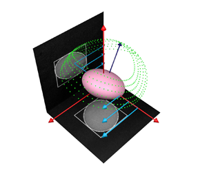
In the absence of inertial and Brownian forces, Jeffery (Reference Jeffery1922) found that the axis of revolution of an axisymmetric rigid particle suspended in a simple shear flow rotates along one of an infinite one-parameter family of closed periodic orbits, known as Jeffery orbits, depicted in figure 1. The time change in orientation is given by the equation for the unit vector  $\boldsymbol {n}$ parallel to the axis of revolution
 \begin{equation} \dot{\boldsymbol{n}} = \boldsymbol{\varOmega} \boldsymbol{\cdot} \boldsymbol{n} + \frac{r^2-1}{r^2+1} [ \boldsymbol{E} \boldsymbol{\cdot} \boldsymbol{n} - \boldsymbol{n} (\boldsymbol{n} \boldsymbol{\cdot} \boldsymbol{E} \boldsymbol{\cdot} \boldsymbol{n})], \end{equation}
where  $r=\ell / a$ is the particle aspect ratio with
 $\ell$ the particle half-length and
 $a$ its radius. The orientation changes fully with the rate of rotation of the flow,
 $\boldsymbol {\varOmega }$, and only by a fraction
 $(r^2-1)/(r^2+1)$ of the rate of strain of the flow,
 $\boldsymbol {E}$. Note that the second term within square parentheses on the right-hand side of (1.1) is just meant to keep
 $|\boldsymbol {n}|=1$. Considering the uniform shearing motion defined by
 $(\dot {\gamma } y, 0,0)$, where
 $\dot {\gamma }$ is the flow shear rate, the orientation of the particle axis of revolution is described by the azimuthal and polar angles,
 $\phi$ and
 $\theta$, shown in figure 1. The Jeffery orbits are of the form (with
 $t = 0$ when
 $\phi = 0$)
 $$\begin{gather} \tan \phi = \frac{1}{r} \tan \left[ \frac{\dot \gamma t}{r + (1/r)}\right], \end{gather}$$
 $$\begin{gather}\tan \theta = \frac{Cr}{(\cos^2 \phi + r^2 \sin^2 \phi)^{1/2}}, \end{gather}$$
where the constant of integration  $C$ is known as the orbit constant. The period of rotation is
 $T_{J}=2{\rm \pi} (r + 1/r)/ \dot {\gamma }$. The rotational motions consist of infinitely many possible spherical ellipses, limited by a tumbling orbit in the
 $(x,y)$ plane on the equator of the sphere
 $(C=\infty )$ and a spinning orbit aligned with the vorticity
 $z$-axis on the pole of the sphere
 $(C=0)$.
Representation of five different Jeffery orbits for a spheroid of aspect ratio  $r=10$. The azimuthal and polar angles,
 $\phi$ and
 $\theta$, are displayed as yellow dashed lines. The trajectories followed by one of the spheroid extremities are obtained by integrating equation (1.1) in time and displayed as dotted lines on the surface of a sphere of radius equal to the particle half-length
 $\ell$. The orbit constant
 $C$ increases across the represented orbits following the dashed arrow, from
 $C=0$ in the
 $z$ axis-aligned log-rolling orbit to
 $C=\infty$ in the tumbling orbit in the (
 $x$,
 $y$) plane. See Figure1.avi in folder Figure_1 in supplementary materials available at https://doi.org/10.1017/jfm.2023.1007 for animations.

Since their formulation, many experimental studies have reported Jeffery orbits for spheroids as well as for other axisymmetric particles such as fibres having  $r \gg 1$ and disks having
 $r\ll 1$ (see e.g. Taylor Reference Taylor1923; Binder Reference Binder1939; Forgacs & Mason Reference Forgacs and Mason1959; Goldsmith & Mason Reference Goldsmith and Mason1962a; Karnis, Goldsmith & Mason Reference Karnis, Goldsmith and Mason1966; Moses, Advani & Reinhardt Reference Moses, Advani and Reinhardt2001; Einarsson et al. Reference Einarsson, Mihiretie, Laas, Ankardal, Angilella, Hanstorp and Mehlig2016). Interestingly, fibres were observed to rotate with a period comparable to that of spheroids with a lower particle aspect ratio (Trevelyan & Mason Reference Trevelyan and Mason1951). Subsequent experiments with disks (Goldsmith & Mason Reference Goldsmith and Mason1962b) and high-aspect-ratio fibres (Anczurowski & Mason Reference Anczurowski and Mason1968) highlighted the shape equivalence existing between spheroidal and cylindrical particles, which could be estimated precisely, moving from a simple linear proportionality (Burgers Reference Burgers1938; Trevelyan & Mason Reference Trevelyan and Mason1951) to a semi-empirical asymptotic theory (Cox Reference Cox1971) and finally to a data-driven formula (Harris & Pittman Reference Harris and Pittman1975). Note that also fore–aft symmetrical particles that possess a discrete rotation symmetry and certain mirror symmetries but do not have a continuous rotation symmetry obey Jeffery's theory, just with different shape parameters, as shown in the seminal paper by Bretherton (Reference Bretherton1962) and more recently by Fries, Einarsson & Mehlig (Reference Fries, Einarsson and Mehlig2017).
In contrast to the case of a suspension of spheres (Einstein Reference Einstein1906, Reference Einstein1911), the first modification to the viscosity of a suspension of spheroids is indeterminate in the limit of the derivation of Jeffery (Reference Jeffery1922), as the particles exist in a dynamical state depending only on their initial orientation and without steady-state preferential orientation. To solve this indeterminacy, Jeffery himself was the first to suggest that spheroids would eventually align with the local vorticity, driven by the terms neglected in his calculations, namely flow and particle inertia. Taylor (Reference Taylor1923) experimentally confirmed this conjecture, whereas different conclusions were later reached by Saffman (Reference Saffman1956), who concluded that small particle inertia breaks the Jeffery orbits for nearly spherical particles, showing that log rolling is stable for nearly spherical prolate particles and unstable for nearly spherical oblate particles. In the following years, few experiments explored the influence of inertia on Jeffery orbits. Preliminary efforts characterised the phenomenon in terms of a slow variation of orbit constant  $C$ among consecutive rotations for negligible particle Reynolds number (Goldsmith & Mason Reference Goldsmith and Mason1962b; Stover & Cohen Reference Stover and Cohen1990). Karnis, Goldsmith & Mason (Reference Karnis, Goldsmith and Mason1963) found that fibres and disks suspended in circular tubes at particle Reynolds numbers
 $Re_p \sim 10^{-4}$ would eventually rotate in the tumbling (
 $C=\infty$) and spinning (
 $C=0$) orbits, respectively. Yet, to the best of our knowledge, no experimental study has produced a rigorous characterisation of the influence of inertia on the Jeffery orbits.
Instead, weak inertial effects have been thoroughly addressed in a number of theoretical works, from Subramanian & Koch (Reference Subramanian and Koch2005, Reference Subramanian and Koch2006) and Einarsson et al. (Reference Einarsson, Candelier, Lundell, Angilella and Mehlig2015a,Reference Einarsson, Candelier, Lundell, Angilella and Mehligb) to Dabade, Marath & Subramanian (Reference Dabade, Marath and Subramanian2016) and Marath & Subramanian (Reference Marath and Subramanian2017, Reference Marath and Subramanian2018). In particular, Subramanian & Koch (Reference Subramanian and Koch2005) examined the inertial effects on fibre motion in simple shear flow, focusing on the slender-body limit (infinite aspect ratio). In this limit, they were able to derive the fibre orbit equations up to  ${{O}}(Re_p)$, where
 $Re_p$ is the Reynolds number based on the fibre length. Their findings were later reproduced both by Einarsson et al. (Reference Einarsson, Candelier, Lundell, Angilella and Mehlig2015a,Reference Einarsson, Candelier, Lundell, Angilella and Mehligb), who exploited asymptotic perturbation theory to extend to small shear Reynolds numbers the range of validity of the equation originally proposed by Saffman for spheroidal particles with arbitrary aspect ratio, and later by Dabade et al. (Reference Dabade, Marath and Subramanian2016), who also analysed inertial effects in terms of modifications to the Jeffery orbit constant. A common conclusion reached by these independent studies is that the most striking effect of fluid and/or particle inertia is to lift the degeneracy of the infinitely many stable Jeffery orbits. This leads to a drift in the trajectory followed by the particles, which are driven towards a limiting stable orbit through consecutive rotations. Prolate spheroids are only pushed towards the tumbling orbit (
 $C = \infty$), whereas the situation is more complex for oblate spheroids which are attracted to either the sole spinning orbit (
 $C = 0$) or both the vorticity-aligned (
 $C = 0$) and the tumbling (
 $C = \infty$) orbits, depending on whether their aspect ratio is larger or smaller than a critical value of approximately 0.14 (Einarsson et al. Reference Einarsson, Candelier, Lundell, Angilella and Mehlig2015b; Dabade et al. Reference Dabade, Marath and Subramanian2016). Interestingly, Marath & Subramanian (Reference Marath and Subramanian2017) also suggested a second-order effect of inertia on the period of rotation, while Rosén et al. (Reference Rosén, Einarsson, Nordmark, Aidun, Lundell and Mehlig2015) discussed the influence of flow confinement over the stability of the tumbling and spinning orbits.
The problem has been also tackled numerically. Several studies based on the lattice-Boltzmann method have considered prolate and oblate spheroids in the near-sphere limit (Qi & Luo Reference Qi and Luo2003; Huang et al. Reference Huang, Yang, Krafczyk and Lu2012; Mao & Alexeev Reference Mao and Alexeev2014). Simulations offer the advantage of easily separating between fluid and particle inertia, characterised by the particle Reynolds number  $Re_p=\rho _f \ell ^2 \dot {\gamma }/\mu$ and the Stokes number
 $St = \rho _p \ell ^2 \dot {\gamma }/\mu = Re_p \rho _p / \rho _f$, respectively, where
 $\rho _p$ is the density of the particle,
 $\rho _f$ that of the fluid and
 $\mu$ the dynamic viscosity. By exploring a wide parameter space (
 $0 < Re_p < 300$ and
 $0 < St < 1200$) for spheroids with moderate aspect ratio
 $2 \leq r \leq 6$, these authors found a good agreement with the theoretical findings of Dabade et al. (Reference Dabade, Marath and Subramanian2016) and Einarsson et al. (Reference Einarsson, Candelier, Lundell, Angilella and Mehlig2015a) at
 $Re_p \sim 10$, but also the emergence of other stable rotation states (spinning, inclined spinning, inclined tumbling or kayaking) for different combinations of increasing particle and flow inertia (Rosén et al. Reference Rosén, Einarsson, Nordmark, Aidun, Lundell and Mehlig2015). Interestingly, these simulations and previous experiments by Zettner & Yoda (Reference Zettner and Yoda2001) reported an increase of the period of rotation with flow inertia, proportional to
 $(Re_{p,cr}-Re_p)^{-0.5}$, where
 $Re_{p,cr}$ is a critical particle Reynolds number above which the considered particles were observed to stop rotating.
In this manuscript, we present the results of an experimental investigation on the rotational dynamics of neutrally buoyant spheroidal and cylindrical particles (both prolate and oblate) subjected to simple shearing flows in the small-inertia regime ( $Re_p= St \lesssim 1$). Since particles and fluid have the same density, we cannot distinguish between specific particle inertia effects and fluid-inertia effects. As we will show, however, our findings are valid regardless of the specific phase that is responsible for the observed inertial bias. The experimental methods are described in § 2. The particles and fluids used are described in § 2.1. The custom-built shearing cell is presented in § 2.2. The multi-view shape-reconstruction method used to obtain direct measurements of the particle orientation is introduced in § 2.3 with details of the data processing in § 2.4 and analysis in § 2.5. The experimental results are presented in § 3. Typical evolutions of the orbits for both oblate and prolate particles are shown in § 3.1. The period of rotation is examined in § 3.2, where a thorough analysis of the equivalence in shape between spheroids and cylinders is proposed. The drift through successive orbits owing to the effect of inertia is analysed in § 3.3 and compared with the asymptotic theories: first in terms of the time variation of the particle orientation vector,
 $\boldsymbol {n}$, (Einarsson et al. Reference Einarsson, Candelier, Lundell, Angilella and Mehlig2015b) and then as the discrete variation of orbit constant,
 $\Delta C$, against
 $C$ (Dabade et al. Reference Dabade, Marath and Subramanian2016). Concluding remarks are drawn in § 4.
2. Experimental methods
2.1. Particles and fluids
Some typical cylindrical and spheroidal particles considered in this study are displayed in figure 2. Their shape is determined by taking multiple pictures with a Hirox RH-2000 digital microscope with a resolution of 221 pixels per mm. Then, 10 measurements are manually made using the software ImageJ to produce a statistical characterisation of their length,  $2 \ell$, and diameter,
 $2a$, and consequently of their aspect ratio,
 $r$, as reported in table 1, where the characteristics of all the particles used are listed. Particles are separated into three different batches according to their production method. The first batch (batch I) comprises two low-aspect-ratio fibres (CYL2, CYL10) and all the (oblate and prolate) spheroids. These particles are produced out of UV-sensitive resin using a stereolithography-3D printer with a resolution of 25
 $\mathrm {\mu }$m and have an estimated density of 1200 kg m
 $^{-3}$. The second batch (batch II) includes two fibres cut from a fishing line and having an estimated density of 1160 kg m
 $^{-3}$. Finally, the last batch (batch III) contains all the disks obtained by laser cutting of rigid Plexiglas sheets having a density of 1180 kg m
 $^{-3}$. Cylinders and spheroids coming from batches I and III are further polished using sandpaper after production: for the former, this is done manually to preserve their sharp edges; for the latter, this is undertaken inside a custom sand-paper box shaken at 1000 rpm by a (Hauschild DAC 150.1 FVZ) speed mixer. Since the typical values of the Young's modulus
 $E$ of the three materials is of the order of a few gigaPascals, the ratio between viscous and elastic forces
 $\mathbb {B} = 8 {\rm \pi}\mu \dot {\gamma } \ell ^4/ (E a^4 {\rm \pi}/4)$ is vanishingly small (
 $\mathbb {B} \sim 10^{-5}$) and the particles do not deform within the flow (Du Roure et al. Reference Du Roure, Lindner, Nazockdast and Shelley2019).
Some typical particles used in the experiments: (a) top view of the disk ‘CYL005’ cut by laser cutter; (b) side view of the spheroidal particle ‘ELL3’; (c) side view of the spheroidal particle ‘ELL06’; (d) side view of the fibre ‘CYL20’ manually cut from fishing line. The yellow dashed curves in panels (a), (b) and (c) represents the circularity of the given ideal shapes.

Characteristics of all the particles used in the experiments. Columns from left to right: code name, shape, mean aspect ratio  $r$, half-length
 $\ell$, radius
 $a$, confinement ratio
 $\kappa$ and identification of the production method.

The fluids used in the experiments are prepared by mixing pure water and citric acid until the solution meets the estimated density of the selected particle. The density of the fluid  $\rho _f$ is sampled by means of a highly accurate (Anton Paar) densimeter with an estimated uncertainty of 4 kg m
 $^{-3}$. Experiments are performed at imposed shear rate
 $\dot {\gamma }$ and the fluid density is constrained to match that of the particle (
 $\rho _p=\rho _f$), yielding
 $Re_p = St$, with
 $Re_p$ and
 $St$ defined in § 1. This implies that inertia is mainly controlled by tuning the fluid viscosity
 $\mu$. This is achieved by adding a certain percentage of Ucon oil
 $^{\rm TM}$ to the solution, which increases its viscosity from that of pure water up to
 $\sim$1 Pa s proportionally to its concentration in our experiments, while also slightly decreasing its density.
2.2. Shearing cell
The shearing cell apparatus is displayed in panel (a) of figure 3. It is located in a room at a controlled temperature of  $23\pm 1\,^{\circ }{\rm C}$ and consists of a small tank (500 mm long, 40 mm wide and 90 mm deep) with 10 mm thick transparent walls on the long sides which have been adapted from the previous work of Metzger & Butler (Reference Metzger and Butler2012). Two metallic cylinders of diameter 20 mm hang from the lid of the tank and are equipped with polylactic acid cylindrical supports that increase their diameter to
 $L_y = 27$ mm. One is free to rotate and the other is coupled to a transmission shaft through a rolling bearing. A transparent belt is kept under tension between the two cylinders, similarly to the photographic roll used in film cameras. It is cut into a rectangular sheet from a 0.1 mm thick flexible Mylar
 $^{\rm TM}$ film and has its extremities kept together by metal staplers. Laser-cut holes in its upper edge enable a gear wheel glued to the rotating cylinder to grip the belt. A rotating motor powered by a DC power supply is connected to the transmission shaft through a drive belt to rotate the gear wheel and drive the transparent belt inside the cell in an infinite loop at constant velocity. The belt is 70 mm tall, extending from nearly the bottom of the shear cell to approximately 15 mm above the free surface.
(a) Picture of the experimental set-up, where the tank filled with fluid between the two sides of the transparent plastic belt is visible (1), together with the rotating motor and the motion transmission system (2) and the two cameras, looking at the  $(x,y)$ flow-gradient plane (3) and at the
 $(x,z)$ flow-vorticity plane (4). (b) Sketch of the output given by the dual-camera video-recording system. The reference frame is defined at the centre of the particle. The azimuthal and polar angles,
 $\phi$ and
 $\theta$, as well as the projected angle,
 $\lambda$, and the three components of the axis-aligned bounding box,
 $\boldsymbol {B}$, are also represented. The two recorded frames are displayed on the corresponding flow-gradient and flow-vorticity planes, to appreciate the contrast between the particle projections and the background as well as the detected particle contours and axis-aligned bounding boxes.

The fluid within the two parallel sides of the belt is submitted to a confined linear shear where the neutral zero-velocity line lies between the two moving walls. The absolute system of reference is defined as  $x$ being the flow direction,
 $y$ the gradient direction and
 $z$ the vorticity direction, parallel to gravity. In our experiments, the origin is always set at the initial position of the particle placed by hand at the centre of the shear flow. The confinement ratio of the particles is defined as the ratio between the particle length and the distance between the two sides of the transparent belt as
 $\kappa = 2\ell / L_y$ (Zettner & Yoda Reference Zettner and Yoda2001). Mean values of the confinement ratio are reported in table 1. These values are similar to that considered in the simulations by Rosén et al. (Reference Rosén, Einarsson, Nordmark, Aidun, Lundell and Mehlig2015), namely
 $\kappa =0.2$. Based on the results of these simulations, a limited confinement effect on some statistical observables may be expected. This is discussed in more detail in §§ 3.3 and 4.
The shearing flow is examined by shedding light onto three different  $(x,y)$ planes at different depths and using particle image velocimetry (PIV). These sections are chosen at least 10 mm below the free surface and above the small unconfined fluid layer laying at the bottom of the cell to characterise a confined region of
 $\sim$30 mm depth where to operate the experiments. The viscosity of the fluid
 $\mu$ is characterised by accurate rheological measurements with an error of
 $0.001$ Pa s on the measurements fully taking into account the real uncertainties. The PIV measurements of the shear rate are performed only for two low and high values of viscosity, as reported in table 2. Then, the effective shear rate for each experiment is estimated by linear interpolation between these two measurements, once the fluid properties have been fixed and its density matched to that of the given particle. Secondary circulations are naturally present in such confined flow and can be characterised by finely tuning the parameters of the PIV. They appear to be insignificant when compared with the mean shear. Also, no significant variation of the shear rate is observed across the depth of the region of interest in the shear cell. To summarise, we observe a linear shear rate in a three-dimensional region the sizes of which are determined by the width of the camera field in the flow direction (
 $L_x = 140$ mm), by the distance between the two inner sides of the transparent plastic belt in the gradient direction (
 $L_y = 27$ mm) and by the depth of the different PIV measurements in the vorticity direction (
 $L_z = 30$ mm).
Shear rate measurements for two low and high values of viscosity. Mean values and uncertainties are calculated over 500 velocity fields obtained by particle image velocimetry. The effective shear rates for the other fluids used are obtained by linear interpolation once the fluid characteristics have been finely tuned to match the density of the particles. It is possible to appreciate the small increase of the shear rate  $\dot {\gamma }$ with increasing viscosity
 $\mu$.

2.3. Measurements
A multi-view video recording system is deployed in the experiments, as shown in panel (b) of figure 3. Jeffery orbits are three-dimensional, but given the axisymmetric nature of the particles, the number of variables that specify the orientation reduces to two. Therefore, measurements of the particle spin were not performed. The objective of this multi-view system is to provide a three-dimensional reconstruction of the orientation of each particle given by its direction vector  $\boldsymbol {n}$. Whereas three or more particle projections would permit a direct resolution (Eberly Reference Eberly1999), we are limited to two complementary images of the axisymmetric particle which are post-processed to reconstruct the orientation as explained in § 2.4.
The cameras are two Allied Prosilica GX1910 cameras, with a resolution of  $1920 \times 1080$ pixels. Both cameras are equipped with a Nikon Micro-Nikkor 55 mm f2.8 objective, imaging the shear cell from a distance of approximately half a metre with a resolution of 20 pixels per mm. As they have their axes perpendicular, these cameras provide two complementary images: one of the flow-vorticity plane and the other of the flow-gradient plane, as seen in figure 3(a). Considering that the depth of field is enhanced to an estimated value of 3 cm, we verified that distortion and diffraction phenomena are negligible by measuring a checker-board patterned object in the flow volume of interest inside the shear cell. The two cameras are controlled by an in-house developed Matlab script.
Experiments are performed as follows. After having filled the cell with the density matched fluid and started shearing, a single particle is manually positioned at the centre of the camera fields, as close as possible to the neutral plane in the middle of the shearing flow. The particle is pre-sheared for a short time to avoid any influence of the positioning operation on its dynamics. Note that, when repeated, this positioning method results in randomly varying initial orientations despite all the care that can be taken. Then, the recording of the two videos is started and the cameras are synchronised by a manually activated light signal. The recording is stopped before the particle leaves the camera fields. Experiments are typically repeated between 5 and 10 times for a given particle at each particle Reynolds number, as reported in table 3. Typically, at least two complete periods of rotation must be observed in order to validate the run. This requirement happened to be rather challenging for the most slender particles.
For each particle type used in the experiments (first column), the particle Reynolds number,  $Re_p$, the number of runs,
 $n_{runs}$, and the mean duration of the shearing normalised by the (experimentally measured) mean period of rotation,
 $\overline {\Delta t_{run}} / T$, are provided.

2.4. Image processing
Each recorded video is processed by an in-house developed Python script based on the Canny method (Canny Reference Canny1986), implemented using the OpenCV library (Bradski Reference Bradski2000). The script performs a simple detection routine based on the contrast between the background and the object to be detected. After having reduced the camera field to a small square section of size  $4 \max (\ell,a) \times 4 \max (\ell,a)$ around the particle, Gaussian blur and manual threshold filters are applied to reduce the noise and improve the contrast by smoothing out possible defects of the transparent plastic belt. At this point, there is a strong intensity gradient between the particle and the background. Identifying this gradient using the Canny edge filter provides the closed contour of the given particle. A least-squared optimisation method yields the orientation angle (fitEllipse function of the OpenCv library), while the extent of the contour in the aligned directions leads to the estimation of its minimum two-dimensional axis-aligned bounding box (boundingRect function of the OpenCv library). By axis-aligned bounding box (AABB hereinafter), we mean the smallest rectangle (parallelepiped when generalising to three dimensions) that is tangent to the particle projection (particle in three dimensions). The three measurements are stored and the script analyses the videos frame by frame. The accuracy of the proposed particle detection method has been evaluated against 8100 virtual images of randomly oriented disks and fibres, with a resolution of 7 pixels over the smallest particle dimension. We found that the Euclidean norm error between theoretical and measured AABBs is below 4 pixels, while the absolute error on the measured angle rarely reached a value above
 $2^{\circ }$.
Two lists of positions, orientations and AABB components of the particle projections onto the flow-gradient and in the flow-vorticity planes in time are the result of the post-processing of each experiment made by the Python script. Then, by a suitable re-scaling, it is possible to combine the information collected by the two cameras and produce three-dimensional measurements of the translation and rotation of the particles. The procedure is non-trivial for the estimation of the orientation of each particle because, as displayed in figure 3, while the particle projection in the  $(x,y)$ plane provides the azimuthal angle
 $\phi$, the projection in the
 $(x,z)$ plane determines the angle
 $\lambda$, which only corresponds to
 $\theta$ in the flow-aligned positions. Therefore, given the possibility of producing long lists of three-dimensional AABBs by knowing the particle orientation vector, we choose a data-driven method to regress the orientation of the particle by a two-camera view system. As detailed in Appendix A, we deploy a simple deep learning model, implemented using Tensorflow and trained over synthetic data, to perform a three-variable regression and estimate the particle orientation vector
 $\boldsymbol {n}$ from the experimentally measured three-dimensional AABBs.
2.5. Data analysis
The data processing of § 2.4 provides the orientation of the axisymmetric particle. This is the key information needed when constructing the Jeffery orbits, discussed in § 3.1, and obtaining the time evolution of the three components of  $\boldsymbol {n}$, discussed in § 3.3. There are two other important quantities: the period of rotation and the orbit constant, described below and used in §§ 3.2 and 3.3, respectively.
Since experimental runs can last up to several particle rotations, the measured projected angles,  $\phi$ and
 $\lambda$, can be interpreted as time series and characterised by Fourier analysis. The Fourier transform of the angular signals can be computed. As a typical example, the power spectra of ten experimental runs are plotted against the frequency in figure 4 for the fibre CYL10. This figure shows that the signal power is coherently resonating around a characteristic frequency, calculated as the frequency
 $f_{max}$ of the peak of each power spectrum. The period of rotation of the given particle,
 $T$, is then estimated as the inverse of this frequency. Measurements are then collected over several runs for a sound statistical characterisation, choosing between the angles
 $\phi$ and
 $\lambda$ according to a minimum squared error criterion. Averages are computed and uncertainties are estimated as standard deviations over all the experimental runs at a given
 $Re_p$.
Power spectra of the two projected angles (a)  $\phi$ and (b)
 $\lambda$, for 10 different experimental runs for the fibre CYL10 of aspect ratio
 $r=9$ at
 $Re_p=0.08$. The insets in each panel show the maximum peak frequency vs the considered runs.

The components of the reconstructed particle orientation vector  $\boldsymbol {n}$ can provide the azimuthal and polar angles, defined as
 $$\begin{gather} n_1 = \sin(\phi)\sin(\theta), \end{gather}$$
 $$\begin{gather}n_2 = \cos(\phi)\sin(\theta), \end{gather}$$
 $$\begin{gather}n_3 = \cos(\theta). \end{gather}$$
Equation (1.3) can then be fitted over the reconstructed values of  $\phi$ and
 $\theta$ to estimate the orbit constant
 $C$ of the given Jeffery orbits, as displayed in figure 5. This is done by a nonlinear least squares minimisation (curvefit function of the Scipy Python library) over an observation window manually centred around each flow-aligned position and with total width comparable to half the period of rotation, producing two separate orbit constant measurements for each Jeffery orbit. Orbit constant variations
 $\Delta C$ are then calculated as discrete differences over one period of rotation. This choice is motivated by a classical approach to the analysis of periodic dynamical systems (Glendinning Reference Glendinning1994), according to which the flow of the orbit constant
 $C$ is obtained by its discrete variations between flow-aligned positions over one period
 $T$. Recalling the orbit coordinates
 $\tau$ and
 $C$ introduced by Leal & Hinch (Reference Leal and Hinch1971), this is equivalent to dropping the temporal dependency of the system (
 $\tau$) and focusing only on the evolution of its phase (
 $C$), similarly to what done in Dabade et al. (Reference Dabade, Marath and Subramanian2016). Therefore, the intensity of the orbit variation
 $\Delta C$ has a sign indicating the direction of the orbit constant motion, i.e. positive when towards the tumbling orbit (
 $C=\infty$) and negative when towards the spinning orbit (
 $C=0$), and a value the magnitude of which quantifies the stability of a given Jeffery orbit (more unstable orbits will experience stronger variations).
Time evolution of the reconstructed angle  $\theta =\arccos n_3$ (black circles). The fitted forms of (1.3) are also plotted as solid lines. The different colours correspond to the estimated values of the orbit constant
 $C$ reported in the legend. The quantity
 $\Delta C$ represents the variation of the orbit constant in each of the measurements.

3. Experimental results
3.1. Jeffery orbits
Typical experimental Jeffery orbits for a fibre of aspect ratio  $r=9$, for an oblate spheroid of aspect ratio
 $r=0.6$ and for the disk of aspect ratio
 $r=0.1$ are shown in figure 6(a,b), (c,d) and (e,f), respectively. The coloured dots represent the intersection of the axis given by the orientation vector
 $\boldsymbol {n}$ with the half-sphere of radius
 $\ell$ for the prolate particles and
 $a$ for the oblate particles, respectively. The location of the intersection was captured during three different experimental runs for each panel and reconstructed as detailed in § 2.4. The corresponding Jeffery orbits at zero inertia are also displayed as solid black lines. They were obtained by integration of (1.1) using the first flow-aligned orientation of each experimental run as initial condition.
Experimental Jeffery orbits at two Reynolds numbers for the fibre CYL10 (top-row panels), the spheroid ELL06 (middle-row panels) and the disk CYL01 (bottom-row panels): (a) fibre,  $r=9.0$,
 $Re_p=0.08$; (b) fibre,
 $r=9.0$,
 $Re_p=1.0$; (c) spheroid,
 $r=0.6$,
 $Re_p=0.02$; (d) spheroid,
 $r=0.6$,
 $Re_p=0.43$; (e) disk,
 $r=0.1$,
 $Re_p=0.05$; (f) disk,
 $r=0.1$,
 $Re_p=1.32$. The particles considered in this figure are shown in the vorticity-aligned position with their orientation vector
 $\boldsymbol {n}$ highlighted in cyan. The coloured dots represent the intersections of the axis given by the orientation vector
 $\boldsymbol {n}$ with the half-sphere of radius
 $\ell$ for the prolate particles and
 $a$ for the oblate particles, respectively. The corresponding Jeffery orbits are also displayed as solid black lines and were obtained by integrating (1.1) from an initial condition given by the first flow-aligned orientation of each experiment. See movies in folder Figure_6_Jeffery_Orbits_animations in supplementary materials for animations.

At low inertia, i.e. for the fibre of panel (a) at  $Re_p=0.08$, the spheroid of panel (c) at
 $Re_p=0.02$ and the disk of panel (e) at
 $Re_p=0.05$, there is no significant change between the successive rotations for runs with different initial conditions, i.e. different orbit constants. The experimental orbits are in good agreement with the theoretical Jeffery orbits, represented by the black spherical ellipses.
As inertia becomes finite, i.e. for the fibre of panel (b) at  $Re_p=1$, the spheroid of panel (d) at
 $Re_p=0.43$ and the disk of panel (f) at
 $Re_p=1.32$, the picture slightly changes. The experimental orbits are still spherical ellipses, but they depart from the zero-inertia orbits as their shapes evolve between successive rotations.
For the fibre of panel (b), the orbits are expanding towards the tumbling orbit ( $C=\infty$) on the equator of the sphere, i.e. in the
 $(x,y)$ flow-gradient plane. It is worth mentioning that the orbits are not equally unstable as the fibre experiences a stronger drift when describing intermediate orbits (run 13) than when close to the rolling (run 14) and tumbling (run 3) cycles.
The oblate particles are also drifting through consecutive orbits, but their behaviour is more complex as two limiting stable orbits exist. As shown in panel (d), the spheroid can either drift to a tumbling orbit ( $C=\infty$) in the plane of shear (run 10) or to a spinning orbit (
 $C=0$), i.e. aligning its orientation vector with the direction of vorticity,
 $z$ (runs 5 and 8). It is interesting to note that the two orbits closer to the pole of the half-sphere (runs 5 and 8) are attracted toward the spinning orbit (
 $C=0$) while the other orbit, which is starting with a much larger orbit constant (run 10), is drawn toward the tumbling orbit (
 $C=\infty$) on the equator of the half-sphere. A similar description holds for the disk of panel (f), which exhibits both consecutive rotations in the tumbling orbit (
 $C=\infty$, run 2) and a systematic drift towards the spinning orbit (
 $C=0$, runs 1 and 9).
A comment is in order regarding the separation between consecutive rotations, which appears larger for the more slender particles, i.e. the fibre with  $r=9$ of panel (b) and the disk with
 $r=0.1$ of panel (f), than in the case of the spheroid with
 $r=0.6$ of panel (d).
3.2. Period of rotation
The dimensionless period of rotation,  $T\dot {\gamma }/2 {\rm \pi}$, of the axisymmetric particles is displayed against particle aspect ratio,
 $r$, in figure 7. The main panel (a) shows all the results obtained for both prolate and oblate particles, while the two smaller panels distinguish between (b) prolate and (c) oblate shapes and focus on the asymptotic limits. The data are obtained by averaging over all the available experiments for all particle Reynolds number (
 $Re_p \lesssim 1$), meaning that we choose in these plots not to take into account any possible influence of inertia on the period of rotation. Such influence will be addressed later at the end of this section. The data are displayed as empty rectangles for cylindrical particles and circles for spheroidal particles and explore a moderate range of aspect ratios (
 $0.05\lesssim r \lesssim 21$). They complement the previous experimental results of Anczurowski & Mason (Reference Anczurowski and Mason1968) for disks and fibres (empty grey diamonds) as well as one prolate spheroid (solid grey
 $\times$), and those of Harris & Pittman (Reference Harris and Pittman1975) for fibres with higher aspect ratio (empty brown pluses), also reported in the figure.
Period of rotation,  $T$, of the axisymmetric particles against the particle aspect ratio
 $r$. The period is made dimensionless using the shear rate
 $\dot {\gamma }$ and normalised by a factor
 $2 {\rm \pi}$. (a) Both prolate and oblate, (b) prolate and (c) oblate particles. The experimental values are displayed as coloured rectangles (cylindrical particles) and circles (spheroidal particles). Each point is the average over all the available experiments for all particle Reynolds numbers (
 $Re_p \lesssim 1$). The theories of Jeffery (Reference Jeffery1922) and Burgers (Reference Burgers1938), the semi-empirical correlation of Cox (Reference Cox1971) and the empirical expression of Harris & Pittman (Reference Harris and Pittman1975) are displayed as a solid black line, a dotted cyan line, a dashed blue line and a dash-dotted pink line, respectively. The experiments of Anczurowski & Mason (Reference Anczurowski and Mason1968) are displayed as empty grey diamonds (cylinders) and one solid
 $\times$ (spheroid), while the data of Harris & Pittman (Reference Harris and Pittman1975) correspond to empty brown plus symbols. See supplementary materials for the directory of the figure including the data and the Jupyter notebook, https://multimediafluids.uam.elogim.com/S0022112023010078/JFM-Notebooks/files/fig7/fig7.ipynb.

The present measurements for the period of spheroidal particles span over two decades of  $r$ around
 $r=1$, extending over the experimental dataset of Anczurowski & Mason (Reference Anczurowski and Mason1968). Their agreement with the theory of Jeffery (Reference Jeffery1922),
 $T_{J} \dot {\gamma } =2{\rm \pi} (r + 1/r)$, displayed as a solid black curve, is excellent. We remark here that the expression just given can be written as
 $2{\rm \pi} /T_J = (\dot {\gamma } /2) \sqrt {1-\varLambda ^2}$ if the Bretherton constant, or shape parameter,
 $\varLambda = (r^2 -1) / (r^2+1)$ is used. In contrast, the measured period of cylindrical particles systematically lies below the Jeffery curve, meaning that the period of a cylinder is always smaller than that of the corresponding spheroid at the same
 $r$. This difference is minimal around
 $r=1$ and increases with increasing slenderness or flatness but not in the same manner. Interestingly, a shorter period of rotation is measured for the disks than for the fibres, as is clearly evidenced by comparing the prolate CYL20 (
 $r=20.5$) and the oblate CYL005 (
 $r=0.05$). These data are in good agreement with those available in the literature (Anczurowski & Mason Reference Anczurowski and Mason1968; Harris & Pittman Reference Harris and Pittman1975).
Since the pioneering work of Trevelyan & Mason (Reference Trevelyan and Mason1951), it has been suggested that an equivalent aspect ratio,  $r_{eq}$, can be found for cylindrical particles to recover the Jeffery period. In particular,
 $r_{eq}$ can be computed from
 $T \dot {\gamma }=2{\rm \pi} (r_{eq} + 1/r_{eq})$ using the measured period of rotation for
 $T$. Different expressions have been proposed for
 $r_{eq}$. In an earlier work for the case of fibres, Burgers (Reference Burgers1938) showed that the disturbance caused by a cylinder of axis ratio
 $r$ will be reproduced by a spheroid of
 $r_{eq}=0.74\,r$, an expression which would eventually diverge at high
 $r$ as well as underestimate the period of rotation in the near-sphere limit. Our measurements for
 $10\lesssim r\lesssim 20$ show good agreement with this proposed equivalence. Later on, by fitting his asymptotic theory to the measurements of Anczurowski & Mason (Reference Anczurowski and Mason1968), Cox (Reference Cox1971) provided an expression for slender cylinders as
 $r_{eq} = 1.24\,r /\sqrt {\log {r}}$. Our data are in good agreement with this formula for
 $r > 5$. Then, Harris & Pittman (Reference Harris and Pittman1975) proposed an unweighted least square log–log fit over their measurements for slender rods leading to
 $r_{eq} = 1.14\,r / r^{0.156}$. They found that Cox's semi-empirical prediction was an overestimate in the asymptotic limit and their power-law function of
 $r$ showed an excellent agreement with all the considered experimental measurements available at that time. This empirical correlation provides an excellent match with our present data for both prolate and oblate cylinders. It is even accurately predicting the additional measurements with the thinnest disk (CYL005, red rectangle in figure 7).
To conclude this section, we move to the influence of inertia on the period of rotation. Figure 8 shows the period of rotation,  $T$, normalised by the Jeffery period,
 $2{\rm \pi} (r_{eq} + 1/r_{eq})/ \dot {\gamma }$, against the particle Reynolds number,
 $Re_p$. The data are now averaged over experimental runs at the same
 $Re_p$ for each particle. While
 $r_{eq}$ is equal to the aspect ratio
 $r$ for the spheroidal particles, its value for the cylindrical particles is determined by solving
 $T \dot {\gamma }=2{\rm \pi} (r_{eq} + 1/r_{eq})$ using their measured period of rotation,
 $T$, at each
 $Re_p$. For both prolate and oblate particles, there is a good collapse of the data around unity, corresponding to the Jeffery period. The data are scattered within
 $\pm 20\,\%$ but do not indicate any systematic trend with increasing inertia. We can conclude that inertia does not affect significantly the period of rotation,
 $T$, for
 $Re_p \lesssim 1$, at least within the range of aspect ratios considered in our study. For much longer (very slender) fibres, some alignment might be observed in the presence of small inertia, as the findings of Subramanian & Koch (Reference Subramanian and Koch2005) seem to suggest, the same being possible for very thin disks, as suggested by the results of Rosén et al. (Reference Rosén, Einarsson, Nordmark, Aidun, Lundell and Mehlig2015).
Period of rotation,  $T$, of the axisymmetric particles against the particle Reynolds number,
 $Re_p$ for: (a) fibres and prolate spheroids and (b) disks and oblate spheroids. The period is now normalised by the Jeffery period,
 $2{\rm \pi} (r_{eq} + 1/r_{eq})/ \dot {\gamma }$. The dotted black line corresponds thus to the Jeffery period within this normalisation. The experiments are displayed as coloured rectangles (cylindrical particles) and circles (spheroidal particles) with the same colour code for the aspect ratios as in figure 7. See supplementary materials for the directory of the figure including the data and the Jupyter notebook, https://multimediafluids.uam.elogim.com/S0022112023010078/JFM-Notebooks/files/fig8/fig8.ipynb.

3.3. Drift
Having previously looked at the general behaviours of the Jeffery orbits in figure 6, we now examine in detail the influence of inertia on the time evolution of each component of the orientation vector  $\boldsymbol {n}$. Figures 9–11 display the three components of
 $\boldsymbol {n}$ in the flow (
 $n_1$), gradient (
 $n_2$) and vorticity (
 $n_3$) directions against the dimensionless time,
 $t\dot {\gamma }$. For clarity of presentation, we have chosen to focus the discussion on a subset of three runs for a typical fibre and a disk at a small but finite
 $Re_p$ and at a larger
 $Re_p$ as well as for an oblate spheroid at a sole moderate
 $Re_p$. We also compare our results with the asymptotic theory of Einarsson et al. (Reference Einarsson, Candelier, Lundell, Angilella and Mehlig2015a) as detailed in § B.1. It is important to stress that, while the theory considers an unbounded system, there is some degree of confinement in the experiments (
 $\kappa \approx 0.2$) which may affect the stability of the orbits (Rosén et al. Reference Rosén, Einarsson, Nordmark, Aidun, Lundell and Mehlig2015). Confinement effects are further discussed in § 4.
Let us first examine the influence of inertia on the dynamics of the fibre with aspect ratio  $r=9$ in figure 9. The general tendency is that the fibre drifts out of the vorticity axis towards the tumbling orbit in the plane of shear, as evidenced by the systematic decrease of
 $n_3$ with successive oscillations. This effect is stronger for intermediate particle orientations, see runs 5 and 8 of panel (a) and runs 13 of panel (b), whereas it may appear somehow irregular for vorticity-aligned orbits, see run 2 of panel (a) and run 14 of panel (b). At small
 $Re_p=0.15$, there is a good agreement between the theory and the experiments, see figure 9(a), suggesting that the range of application of the asymptotic theory of Einarsson et al. (Reference Einarsson, Candelier, Lundell, Angilella and Mehlig2015a) can be extended to finite values of
 $Re_p \sim O(10^{-1})$ in the case of the fibres. The agreement is inevitably lost at larger values, e.g.
 $Re_p \sim O(1)$. At such
 $Re_p$, a faster drift toward the tumbling orbit is systematically obtained as compared with the experiments, as can be seen from figure 9(b), in particular for the case of run 13.
Evolution of the components of the orientation vector  $\boldsymbol {n}$, displayed as vertically aligned panels for 3 typical runs against the dimensionless time
 $t\dot {\gamma }$, for the fibre CYL10 with aspect ratio
 $r=9$ and confinement ratio
 $\kappa =0.19$: (a)
 $Re_p=0.15$; (b)
 $Re_p=1.0$. Comparison with the theory of Einarsson et al. (Reference Einarsson, Candelier, Lundell, Angilella and Mehlig2015a), presented in § B.1 is also given as black dashed lines. See supplementary materials for the directory of the figure including the data and the Jupyter notebook, https://multimediafluids.uam.elogim.com/S0022112023010078/JFM-Notebooks/files/fig9/fig9.ipynb.

The discussion is now repeated for the disk with aspect ratio  $r=0.05$ in figure 10. Most of the runs show a tendency for the disk to drift towards the vorticity axis, i.e. to move towards the spinning orbit where the particle lays flat in the flow-gradient plane. However, a few runs (with carefully tuned initial conditions) show disks that are just tumbling with their axis in the plane of shear. This confirms that, unlike prolate particles (which are always driven towards the sole limiting tumbling orbit), oblate particles can drift towards two different orbits, the spinning or the tumbling orbits, depending upon their initial orientations. Whereas the theory of Einarsson et al. (Reference Einarsson, Candelier, Lundell, Angilella and Mehlig2015a) successfully predicts the existence of two limiting orbits, it gives a much stronger overestimation of the drift through consecutive orbits for disks than for fibres, even for the smallest values of
 $Re_p$ studied. This seems to imply that the range of application of the asymptotic theory is more limited in the oblate case than in the prolate case. This is clear in figure 10(a) for
 $Re_p=0.24$, but becomes even more evident in figure 10(b) for
 $Re_p=0.80$. At this larger
 $Re_p$, the theory predicts a rapid shift towards aligned positions while the experiments still show rotational behaviours.
Evolution of the components of the orientation vector  $\boldsymbol {n}$, displayed as vertically aligned panels for 3 typical runs against the dimensionless time
 $t\dot {\gamma }$, for the disk CYL005 with aspect ratio
 $r=0.05$ and confinement ratio
 $\kappa =0.19$: (a)
 $Re_p=0.24$; (b)
 $Re_p=0.8$. Comparison with the theory of Einarsson et al. (Reference Einarsson, Candelier, Lundell, Angilella and Mehlig2015a), presented in § B.1 is also given as black dashed lines. See supplementary materials for the directory of the figure including the data and the Jupyter notebook, https://multimediafluids.uam.elogim.com/S0022112023010078/JFM-Notebooks/files/fig10/fig10.ipynb.

Finally, we consider the oblate spheroid ELL06 with  $r=0.6$ at moderate
 $Re_p=0.43$ in figure 11. At first glance, no remarkable difference emerges with regards to the slender disk CYL005, displayed in figure 10. This spheroid either tumbles in the plane of shear (run 10) or slowly drifts to the spinning orbit (runs 8 and 5). However, in addition to the already discussed discrepancy of the drift, there is a notable difference between the theory of Einarsson et al. (Reference Einarsson, Candelier, Lundell, Angilella and Mehlig2015a) and the experiments regarding the dynamics of this nearly spherical oblate spheroid. For this type of particle, the asymptotic theory only predicts the drift to an attracting spinning orbit at
 $Re_p \ll 1$. This is further discussed in connection to confinement effects in § 4.
Evolution of the components of the orientation vector  $\boldsymbol {n}$, displayed as vertically aligned panels for 3 typical runs against the dimensionless time
 $t\dot {\gamma }$, for the oblate spheroid ELL06 with aspect ratio
 $r=0.6$ and confinement ratio
 $\kappa =0.17$ at particle Reynolds number
 $Re_p=0.43$. Comparison with the theory of Einarsson et al. (Reference Einarsson, Candelier, Lundell, Angilella and Mehlig2015a), presented in § B.1 is also given as black dashed lines. See supplementary materials for the directory of the figure including the data and the Jupyter notebook, https://multimediafluids.uam.elogim.com/S0022112023010078/JFM-Notebooks/files/fig11/fig11.ipynb.

As previously mentioned in § 1, the separation between the two limiting orbits for the oblate particles is predicted to depend on their initial orientations but also on their aspect ratio (Einarsson et al. Reference Einarsson, Candelier, Lundell, Angilella and Mehlig2015b; Dabade et al. Reference Dabade, Marath and Subramanian2016). To examine this difference in drift more closely and avoid the ambiguity of an arbitrary initial condition, we calculate the change in the orbit constant in a single Jeffery period as done in Dabade et al. (Reference Dabade, Marath and Subramanian2016). As detailed in § 2.5, this implies the fitting of our experimental measurements to estimate the local values of the orbit constant  $C$ before taking discrete differences
 $\Delta C$ over each period of rotation. The results are shown in figure 12, where the normalised change in the orbit constant in a single period,
 $Re_p^{-1}\Delta C/(C^2+1)$, is plotted against the normalised orbit constant
 $C/(C+1)$ for all the experiments. Measurements referring to different values of
 $Re_p$ are identified by different colours. The values
 $C/(C + 1) = 0$ and
 $C/(C + 1) = 1$ correspond to the spinning and tumbling modes, respectively. Following Dabade et al. (Reference Dabade, Marath and Subramanian2016), to keep the drift finite in the near-sphere limit, the normalisation for
 $\Delta C$ also uses a factor depending on the particle eccentricity:
 $\xi _0 = \sqrt {1/(1-1/r^2)}$ for the prolate particles and
 $\xi _0 = \sqrt {1/(1-r^2)}$ for the oblate particles.
Discrete variation of the orbit constant over one period,  $\Delta C$, against the orbit constant
 $C$. Results refer to the following particle types (characterised by different colours for the varying
 $Re_p$): (a) disk CYL005 (
 $r=0.05$ and
 $\kappa =0.19$); (b) disk CYL009 (
 $r=0.1$ and
 $\kappa =0.11$); (c) disk CYL01, (
 $r=0.11$ and
 $\kappa =0.21$); (d) spheroid ELL06,
 $r=0.56$ and
 $\kappa =0.17$); (e) spheroid ELL3, (
 $r=2.67$ and
 $\kappa =0.19$); (f) fibre CYL10, (
 $r=9.01$ and
 $\kappa =0.19$). The drift is normalised to keep its value finite in the near-sphere limit as in Dabade et al. (Reference Dabade, Marath and Subramanian2016), thus yielding a better comparison with their theory (black dashed line and black solid line in the slender limit). The predicted critical orbit constant
 $C^* = \sqrt {35}$, i.e.
 $C^*/(C^*+1) \simeq 0.86$, separating the basins of attraction in the slender disk limit is also displayed as a dash-dotted grey line (Dabade et al. Reference Dabade, Marath and Subramanian2016). Data are collected over all the available experiments at a given
 $Re_p$ (up to 10 runs), measuring the orbit constant and its variation as described in § 2.5. See supplementary materials for the directory of the figure including the data and the Jupyter notebook, https://multimediafluids.uam.elogim.com/S0022112023010078/JFM-Notebooks/files/fig12/fig12.ipynb.

Figure 12 displays results for the following cases: the thinnest disk with  $r=0.05$ in panel (a), two disks having similar
 $r$ but two different confinement ratios in panels (b) (
 $r=0.1, \kappa =0.1$) and (c) (
 $r=0.11, \kappa =0.2$) and a thicker oblate spheroid with
 $r=0.56$ in panel (d). Also included are the results for two prolate particles: a prolate spheroid with
 $r=2.7$ in panel (e) and a slender fibre with
 $r=9$ in panel (f). These data are compared with the theoretical prediction of Dabade et al. (Reference Dabade, Marath and Subramanian2016) considering both particle and fluid inertia (
 $St=Re_p$ in the present neutrally buoyant case) as detailed in § B.2.
Despite the rather large scatter of the data, there are some clear trends and qualitative agreements with theoretical predictions. Prolate particles experience positive increments of the orbit constant, which drive them towards tumbling motion ( $C=\infty$, namely
 $C/(C+1)=1$), while oblate particles experience negative variations as they are mostly attracted to the vorticity-aligned orbit (
 $C=0$, namely
 $C/(C+1)=0$). Moreover, as revealed from the scales of the ordinate axes, the drift intensity
 $\Delta C$ increases with the aspect ratio
 $r$, as more slender objects experience more unstable Jeffery orbits.
The oblate particles not only drift towards the spinning orbit but also to the tumbling orbit, as evidenced by the clustering of points around zero and slightly above for orbit constants  $C \gtrsim \sqrt {35}$, namely
 $C/(C+1) \gtrsim 0.86$, as computed by Dabade et al. (Reference Dabade, Marath and Subramanian2016), see panels (a) to (c). This is in stark contrast with the strong incline taken by the fibre of aspect ratio
 $r=9$ in panel (f) when leaving the spinning orbit (
 $C/(C+1)=0$) which is unstable for this prolate particle.
An interesting behaviour is observed in panel (d) for the oblate spheroid with  $r=0.6$, a value well above the predicted critical aspect ratio of approximately
 $0.14$ for which only drift toward the spinning motion is anticipated. As evidenced in figure 11, this particle is still experiencing tumbling and spinning orbits, in contradiction to theoretical predictions. The critical orbit constant seems also to have moved as positive increments of orbit constant are observed at
 $C \lesssim \sqrt {35}$, i.e.
 $C/(C+1) \lesssim 0.86$, in particular for the higher
 $Re_p$. Similar behaviour is observed for the disk with
 $r_{eq}=0.18$ in panels (b) and (c), which correspond to different confinements. This may suggest a wider region of attraction for the tumbling mode.
The influence of confinement is clearly visible between panels (b) and (c), where are shown two disks at a comparable  $r \approx 0.1$ but differing confinement ratios,
 $\kappa =0.11$ and
 $\kappa = 0.21$. The smaller disk is in better agreement with the theory than the large disk, having a twofold increase of confinement ratio, where the drift is less intense than that predicted by Dabade et al. (Reference Dabade, Marath and Subramanian2016) for an unconfined viscous shear flow.
Finally, we address the scaling of the drift intensity with the particle Reynolds number. Clearly, experiments at higher particle Reynolds number ( $Re_p \approx 1$) do not collapse with those at smaller
 $Re_p$. Despite the large scatters, this is particularly evidenced in panels (a,c,d) for oblate objects, where the intensity of the drift is weaker for the larger
 $Re_p$. This suggests a saturation effect above a certain inertial threshold.
4. Concluding remarks
We have examined the rotation of axisymmetric particles suspended in a simple shear flow when inertia is progressively increased up to particle Reynolds number  $Re_p \simeq 1$. A custom-built shearing cell and a multi-view reconstruction method have been used to obtain direct measurements of the orientation and period of rotation of ideal bodies such as spheroids but also bodies of practical interest such as cylinders with different aspect ratios. This system is rather flexible and is amenable to studying the alignment of small bodies with different shapes in simple shearing flows.
The first important result is that the axisymmetric particles still rotate with the Jeffery period in this small-inertia regime. Our results also complement the data available in the literature (Anczurowski & Mason Reference Anczurowski and Mason1968; Harris & Pittman Reference Harris and Pittman1975) and provide a connection with those of Zettner & Yoda (Reference Zettner and Yoda2001) at higher  $Re_p$, showing that the period of rotation of a cylinder is smaller than that of a spheroid with the same aspect ratio. An equivalent spheroidal aspect ratio can be inferred to recover the Jeffery period in the case of cylinders. Our results show that the empirical expression of Harris & Pittman (Reference Harris and Pittman1975) remains the best prediction for this equivalent aspect ratio, which we were able to validate over one further decade of slender oblate particles compared with available literature results.
The second major output is that we observe an irreversible drift across Jeffery orbits towards attracting limiting cycles. This drift is due to weak inertial effects, and its occurrence confirms, at least qualitatively, the asymptotic theories of Einarsson et al. (Reference Einarsson, Candelier, Lundell, Angilella and Mehlig2015b) and Dabade et al. (Reference Dabade, Marath and Subramanian2016). It is important to stress before proceeding to any comparison below that these theories are meant to be valid for  $Re_p\ll 1$ as well as at infinite distance from walls. Clearly, some deviations between their predictions and experimental results begin to appear as one moves away from their range of validity as discussed below.
Our measurements indicate that prolate particles are uniquely driven towards a tumbling motion in the flow-gradient plane regardless of their initial orientation and aspect ratio. For small but finite  $Re_p$, i.e. typically up to
 ${O}(10^{-1})$ in our experiments, there is a good quantitative agreement with the theories. For larger
 $Re_p$, i.e. of
 ${O}(1)$ in our experiments, a saturation of the phenomenon is observed and the asymptotic theories predict a faster drift toward the tumbling orbit. This is expected since these theories are strictly valid only for
 $Re_p\ll 1$ and cannot be expected to describe the dynamics at an
 $Re_p$ of order unity or larger, as also discussed in Rosén et al. (Reference Rosén, Einarsson, Nordmark, Aidun, Lundell and Mehlig2015).
In stark contrast to prolate particles, which only possess a single attracting orbit, oblate particles are observed to drift towards two different orbits, the spinning orbit or the tumbling orbit, depending upon their initial orientation. Whereas the theories of Einarsson et al. (Reference Einarsson, Candelier, Lundell, Angilella and Mehlig2015b) and Dabade et al. (Reference Dabade, Marath and Subramanian2016) do predict the existence of two limiting orbits, their overestimation of the drift through consecutive orbits is more severe and even seen for small  $Re_p$ of
 ${O}(10^{-1})$, as also discussed in Rosén et al. (Reference Rosén, Einarsson, Nordmark, Aidun, Lundell and Mehlig2015) when the theory is compared with direct numerical simulations (DNS) results. This may suggest that the predictive capabilities of the theories in the small-inertia regime are more limited for oblate particles and that their range of application at finite
 $Re_p$ is narrower than for prolate particles. We remark here that part of the observed overestimation may be ascribed to unavoidable confinement effects (Rosén et al. Reference Rosén, Einarsson, Nordmark, Aidun, Lundell and Mehlig2015), which tend to lower the drift intensity and thus introduce a small bias in the experimental measurements. Again, it seems that these effects do affect more the oblate particles.
There is a notable discrepancy between the experiments and the predictions of Einarsson et al. (Reference Einarsson, Candelier, Lundell, Angilella and Mehlig2015b) and Dabade et al. (Reference Dabade, Marath and Subramanian2016) regarding the stability of the tumbling orbit for oblate particles. A bifurcation toward a single stable spinning orbit above a critical aspect ratio of approximately  $0.14$ is not observed, suggesting a wider basin of attraction for the tumbling mode in the experiments for small
 $Re_p$ of
 ${O}(10^{-1})$ up to
 ${O}(1)$. The time-resolved simulations of Rosén et al. (Reference Rosén, Einarsson, Nordmark, Aidun, Lundell and Mehlig2015) having a confinement of
 $\kappa =0.2$ have shown a bifurcation between stable and unstable tumbling for a critical aspect ratio of approximately 0.13 at
 $Re_p=1$, in fair agreement with the prediction 0.14 of the asymptotic theories. Rosén et al. (Reference Rosén, Einarsson, Nordmark, Aidun, Lundell and Mehlig2015) even tracked the bifurcation for larger
 $Re_p$, showing that it can survive up to
 $Re_p=5$, see the bifurcation diagram of their figure 4. Our experimental results for similar confinement (
 $\kappa =0.2$) and even those with smaller confinement (
 $\kappa =0.1$) still exhibit stable tumbling modes. While this finding is intriguing, it seems reasonable to assume that it cannot be attributed to confinement.
Overall, our results indicate that inertia plays a significant role in breaking the indeterminacy of the Jeffery orbits for the prolate particles, while we still observe the existence of two limiting orbits for the oblate particles. This finding has deep consequences for the steady-state rheology of suspensions of axisymmetric particles in a viscous dilute regime, i.e. when particle–particle interactions are negligible. Indeed, prolate particles will eventually drift toward the tumbling orbit, aligning asymptotically with the mean flow direction. Conversely, the effective viscosity of a suspension of oblate particles will always depend on their initial orientation and regardless of their aspect ratio, i.e. not only in the lower near-sphere limit ( $0.14< r<1$) as predicted by Dabade et al. (Reference Dabade, Marath and Subramanian2016). Of course, hydrodynamic and direct particle–particle interactions come into play and change the picture as soon as semi-dilute and concentrated suspensions are considered (Butler & Snook Reference Butler and Snook2018).
A final comment is in order about the importance of including the effect of both the fluid and particle inertia in the numerical calculation of the rotational dynamics of axisymmetric particles suspended in complex flows, e.g. turbulent flows. In a turbulent flow, the modified rotation rate (see (B1)) might affect the distribution of particle orientations (Sheikh et al. Reference Sheikh, Gustavsson, Lopez, Lévêque, Mehlig, Pumir and Naso2020). In homogeneous isotropic turbulence, axisymmetric prolate (respectively oblate) particles were seen to align with (respectively perpendicular to) the local vorticity vector, following the local flow stretching in a mostly spinning (respectively tumbling) rotational state (Byron et al. Reference Byron, Einarsson, Gustavsson, Voth, Mehlig and Variano2015; Ni et al. Reference Ni, Kramel, Ouellette and Voth2015). Accounting for the inertial torques would strengthen the influence of the local stretching, even if one might argue under which conditions the inertial contribution becomes relevant given the intermittent nature of the flow. One may indeed need to compare the drift time (of the typical order of a few periods of rotation) with the typical time of the flow velocity fluctuations. The picture is even more complex in bounded turbulence, where the strong near-wall shear causes axisymmetric particles to follow the local flow stretching but aligns the vorticity vector in the spanwise direction (Zhao & Andersson Reference Zhao and Andersson2016). In this case, inertial torques could especially modify the orientation statistics of oblate particles, which tend to align normal to the wall, with possible consequences for drag reduction (Wang, Xu & Zhao Reference Wang, Xu and Zhao2021).
Supplementary material and movies
Supplementary material, movies and Computational Notebook files are available at https://doi.org/10.1017/jfm.2023.1007. Computational Notebooks can also be found online at https://multimediafluids.uam.elogim.com/S0022112023010078/JFM-Notebooks.
Acknowledgements
We thank N.K. Marath and G. Subramanian for providing detailed information on their calculation for the drift of oblate spheroids.
Funding
D.D.G. acknowledges the Universitá Italo-Francese, Bando Vinci 2021, cap. 2, progetto C2-257 ‘Fibre flessibili in flusso turbolento ad elevato numero di Reynolds” for the generous funding.
Declaration of interests
The authors report no conflict of interest.
Appendix A. Three-dimensional particle orientation estimation
A.1. Three-dimensional AABB calculation for cylinders and spheroids
In this section we briefly describe the geometrical relations that provide the AABB  $\boldsymbol {B}$ for cylindrical and spheroidal particles, having imposed their orientation vector
 $\boldsymbol {n}$. The relation is straightforward for cylinders, whose projection corresponds to the sum of a line and two capping circles (Quilez Reference Quilez2016). The eccentricity
 $e$ of these two circles is defined as
 \begin{equation} e = a \boldsymbol{\cdot} \sqrt{1-\boldsymbol{n}\boldsymbol{\cdot} \boldsymbol{n}} . \end{equation}
Given the centre points of the capping circles,  $\boldsymbol {p_a}$ and
 $\boldsymbol {p_b}$,
 $\boldsymbol {B}$ is obtained by maximising the only possible orientation extension
 \begin{equation} \boldsymbol{B} = \max ((\boldsymbol{p_a}+e),(\boldsymbol{p_b}+e)) - \min ((\boldsymbol{p_a}-e),(\boldsymbol{p_b}-e) ) . \end{equation}
Performing the same calculation for spheroidal particles is slightly more complex, in view of the lack of sharp edges. A generic spheroid that can only rotate but not translate may be represented as a diagonal matrix. If the spheroid is initially aligned with the  $z$ axis such that its orientation vector is
 $\boldsymbol {n} = (0,0,1)$, then the matrix reads as follows:
 \begin{equation} \bar{\mathbf{O}} =\begin{bmatrix} a^{{-}2} & 0 & 0 \\ 0 & a^{{-}2} & 0 \\ 0 & 0 & (a \cdot r)^{{-}2} \\ \end{bmatrix} . \end{equation}
Neglecting the spin, any generic orientation attained by the spheroid can be determined by a combination of the two polar angles  $\phi$ and
 $\theta$
 \begin{equation} \boldsymbol{n}= (\sin{\phi}\sin{\theta}, \cos{\phi}\sin{\theta}, \cos{\theta} ) . \end{equation}
It is straightforward to build a rotation matrix that correlates the initial orientation of the spheroid to the new one through equation (A4). Therefore, the quadratic form of the spheroid will also be rotated according to the new orientation as follows:
 \begin{equation} \bar{\boldsymbol{Q}} = \bar{\boldsymbol{R}} \boldsymbol{\cdot} \bar{\boldsymbol{O}} \boldsymbol{\cdot} \bar{\boldsymbol{R}}^T . \end{equation}
Given the matrix  $\bar {\boldsymbol {Q}}$, in Appendix A.3 we demonstrate that taking the square root of the diagonal components of its inverse yields the halved sides of the AABB
 \begin{equation} \boldsymbol{B}_i = 2 \boldsymbol{\cdot} \sqrt{{\bar{\boldsymbol{Q}}_{i,i}}^{{-}1}} . \end{equation}
The procedure just described is repeated over  $360 \times 360 = 129\,600$ possible combinations of values of
 $\phi$ and
 $\theta$, in order to discretise any possible orientation in the first quadrant of the three-dimensional Cartesian system. This results in a resolution of
 $0.25^{\circ }$ for each angle. Calculations are scripted in Python to generate extended data sets of AABBs and their corresponding orientation vectors. The corresponding scripts are provided in the supplementary materials.
A.2. Orientation reconstruction by multi-variable regression
The relation between the AABB  $\boldsymbol {B}$ and the particle orientation vector
 $\boldsymbol {n}$ is nonlinear and known in a closed form only for the inverse transformation. Therefore, to solve the direct transformation, we choose a data-driven approach.
A deep learning model is trained using synthetic data generated geometrically, as described in the previous section. The model is implemented as a neural network in TensorFlow (Abadi Reference Abadi2015), and performs a multi-variable regression, where the input is an experimentally measured AABB and the output is the corresponding orientation vector  $\boldsymbol {n}$. Hidden dense layers are made of 256 fully connected weights, introducing nonlinearity through the relu activation function. Typically, one hidden layer would be sufficient for the regression of the most slender shapes, however, three layers seem preferable to be able to deal also with the nearly spherical objects, e.g. the spheroid ELL06. Normalisation of the Euclidean norm of the output orientation vector
 $\boldsymbol {n}$ is finally ensured by a dedicated lambda layer. The model is compiled and normally trained over at least 20 epochs by minimising a custom loss function (CLF), which calculates the Euclidean norm of the difference between the true and predicted values of the orientation vector
 $\boldsymbol {n}$
 \begin{equation} {\rm CLF} = \sqrt{\sum_{i=1}^{3} ( \boldsymbol{n}_{true,i} - \boldsymbol{n}_{pred,i} )^2 }. \end{equation}
In addition, the CLF strongly penalises any prediction yielding non-physical, lower-than-zero values for the orientation vector components. The chosen optimisation method is Adam, which is a randomised batched gradient descent method. A random  $20\,\%$ splitting of the data set between training and testing samples is selected for the training. As displayed in figure 13, the regression for a fibre of aspect ratio
 $r=9.01$ (CYL10) is highly reliable and yields precise estimations of the three components of the orientation vector
 $\boldsymbol {n}$. It is important to stress that the lack of availability of previously measured similar experiments prevents us from further testing the model. The Python script used to estimate the particle orientation vector
 $\boldsymbol {n}$ from its AABBs is provided in the supplementary materials.
Predicted values against true values of the orientation vector  $\boldsymbol {n}$ obtained applying the deep learning model described in Appendix A.2 to a fibre with aspect ratio
 $r=9.01$ (CYL10): (a)
 $n_1$ along
 $x$, (b)
 $n_2$ along
 $y$, (c)
 $n_3$ along
 $z$.

A.3. Relation between the AABB of a spheroid and the principal diagonal terms of its matrix of coefficients
Given a generic  $n$-dimensional hyper-spheroid
 $\mathcal {E}$
 \begin{equation} \mathcal{E} = \{ x \in \mathbb{R}^n\, |\, (x - c)^T Q^{{-}1}(x - c) \leq 1 \} , \end{equation}
where  $c \in \mathbb {R}^n$ is the vector defining the centre of the spheroid and
 $Q$ is a positive definite matrix of coefficients, and writing
 $g(x)=(x - c )^T Q^{-1}(x - c )$, the vector field orthogonal to the shell of the spheroid is
 \begin{equation} \boldsymbol{\nabla} g(x) = 2 Q^{{-}1} (x - c). \end{equation}
Considering the  $i$th axis and the corresponding projection matrix
 $P_i = e_i e_i^T$, the orthogonal vector field
 $\boldsymbol {\nabla } g(x)$ and its projection
 $P_i \boldsymbol {\nabla } g(x)$ will satisfy the condition
 \begin{equation} \boldsymbol{\nabla} g(x) = P_i \boldsymbol{\nabla} g(x) , \end{equation}
at the two points where the spheroid  $\mathcal {E}$ touches the (smallest) bounding box, namely the smallest AABB. The above condition is equivalent to
 \begin{equation} (I_n - P_i) \underbrace{Q^{{-}1} (x-c)}_{{\equiv} y} = 0_n , \end{equation}
where the entry  $y_i$ will be the only non-zero value, i.e.
 $y = t e_i$, or
 $x = c + t Q e_i$. Intersecting this line with the boundaries of the spheroid,
 $t$ can be obtained as follows:
 \begin{equation} t^2 = (e_i^T Q e_i)^{{-}1} = q_{ii}^{{-}1} , \end{equation}
where  $q_{ii}$ is the
 $i$th entry of the inverse of the matrix
 $Q$. Therefore, the shell of the
 $i$th projection of the spheroid will touch the smallest AABB at the following two points:
 \begin{equation} x_i = c_i \pm \frac{1}{\sqrt{q_{ii}}} e_i^T Q e_i = c_i \pm \frac{q_{ii}}{\sqrt{q_{ii}}} = c_i \pm \sqrt{q_{ii}}. \end{equation}
Appendix B. Comparison with small-inertia theories
B.1. Model of Einarsson et al. (Reference Einarsson, Candelier, Lundell, Angilella and Mehlig2015a)
Einarsson et al. (Reference Einarsson, Candelier, Lundell, Angilella and Mehlig2015a) characterised the influence of inertia on Jeffery orbits as additional terms to (1.1), which then reads as
 \begin{align} \dot{\boldsymbol{n}} &= \boldsymbol{\varOmega} \boldsymbol{\cdot} \boldsymbol{n} + \frac{r^2-1}{r^2+1} [ \boldsymbol{E} \boldsymbol{\cdot} \boldsymbol{n} - \boldsymbol{n} (\boldsymbol{n} \boldsymbol{\cdot} \boldsymbol{E} \boldsymbol{\cdot} \boldsymbol{n})] + \beta_1 ( \boldsymbol{n} \boldsymbol{\cdot} \boldsymbol{E} \boldsymbol{\cdot} \boldsymbol{n} ) \mathbb{P}(\boldsymbol{E}\boldsymbol{\cdot} \boldsymbol{n})\nonumber\\ &\quad + \beta_2 ( \boldsymbol{n}\boldsymbol{\cdot} \boldsymbol{E} \boldsymbol{\cdot} \boldsymbol{n} ) \boldsymbol{\varOmega} \boldsymbol{\cdot} \boldsymbol{n} + \beta_3 \mathbb{P} (\boldsymbol{\varOmega} \boldsymbol{\cdot}\boldsymbol{E}\boldsymbol{\cdot} \boldsymbol{n}) + \beta_4 \mathbb{P} (\boldsymbol{E} \boldsymbol{\cdot} \boldsymbol{E} \boldsymbol{\cdot} \boldsymbol{n}) , \end{align}
where  $\mathbb {P} (\boldsymbol {x}) = \boldsymbol {x} - (\boldsymbol {n} \boldsymbol {\cdot } \boldsymbol {x}) \,\boldsymbol {n}$ is an operator that projects components in the
 $\boldsymbol {n}$-direction. The first two terms on the right-hand side of (B1) correspond to the original Jeffery equation while the last four terms, each containing a scalar coefficient
 $\beta _i$, are the inertia-related terms. The coefficients
 $\beta _i$ are functions of the particle aspect ratio, provided graphically in figure 2 of Einarsson et al. (Reference Einarsson, Candelier, Lundell, Angilella and Mehlig2015b) for
 $Re_p = St$ and reported here in figure 14 for the CYL10 case, using the equivalent aspect ratio for cylinders. Equation (B1) is integrated in time using the odeint function of the Scipy Python library. The initial conditions are provided by the first flow-aligned orientation measured in the CYL10 experimental run. The Python script used to solve for (B1) is provided in the supplementary materials.
The  $\beta _i$ coefficients of (B1) as given in figure 2 of Einarsson et al. (Reference Einarsson, Candelier, Lundell, Angilella and Mehlig2015b). As an example, for the fibre CYL10, the coefficients
 $\beta _i$ are chosen at the intersection between the dotted vertical line at
 $r_{eq}= 7.4$ with the respective curves.

B.2. Model of Dabade et al. (Reference Dabade, Marath and Subramanian2016)
Dabade et al. (Reference Dabade, Marath and Subramanian2016) characterise the inertia-driven drift from the Jeffery orbits through consecutive rotations by means of discrete variations of the orbit constant  $\Delta C$ in a single Jeffery period. For particle inertia, this is given in their (5.19) in terms of the eccentricity:
 $\xi _0 = \sqrt {1/(1-1/r^2)}$ for the prolate and
 $\xi _0 = \sqrt {1/(1-r^2)}$ for the oblate particles. The eccentricity parameter
 $\xi _0$ is calculated using the physical particle aspect ratio,
 $r$, for the spheroids and the equivalent particle aspect ratio,
 $r_{eq}$, for the cylinders, obtained by averaging over all the available experiments. Then, the integrals
 $I_i,J_i$ are provided in Appendix C, while the prolate
 $F_i^p,G_i^p$ coefficients come from their (5.7)–(5.12). Following Dabade et al. (Reference Dabade, Marath and Subramanian2016) to obtain the oblate coefficients, one needs first to multiply the prolate coefficients by the squared length-scale to obtain their dimensional form. Then the transformation prolate-to-oblate must be applied (
 $\xi _0 <->i (\xi _0^2-1)^{0.5}$), before returning to dimensionless variables by dividing by the squared length scale, as described below (5.12) of Dabade et al. (Reference Dabade, Marath and Subramanian2016). The fluid-inertia drift is still obtained from (5.19), where
 $St$ is replaced by
 $Re_p$ and the
 $F_i^f,G_i^f$ coefficients are given in (6.1)–(6.8). The Python script used to calculate the discrete orbit variation
 $\Delta C$ as in Dabade et al. (Reference Dabade, Marath and Subramanian2016) is provided in the supplementary materials.



