1. Introduction
The upper ocean is host to energetic flows at scales smaller than the order 100 km mesoscale eddies. Sharp surface fronts associated with strong along-front currents are generated in high-resolution numerical simulations (e.g. Capet et al. Reference Capet, McWilliams, Molemaker and Shchepetkin2008b ; Klein et al. Reference Klein, Hua, Lapeyre, Capet, Le Gentil and Sasaki2008) and are observed in the wintertime midlatitude ocean (Shcherbina et al. Reference Shcherbina, D’Asaro, Lee, Klymak, Molemaker and McWilliams2013; Callies et al. Reference Callies, Ferrari, Klymak and Gula2015). These submesoscale flows at scales 1–100 km are associated with large vertical fluxes of both physical and biogeochemical tracers that have been argued to regulate the oceanic heat and carbon uptake in global warming scenarios (Capet et al. Reference Capet, McWilliams, Molemaker and Shchepetkin2008b ; Klein & Lapeyre Reference Klein and Lapeyre2009; Ferrari Reference Ferrari2011; Lévy et al. Reference Lévy, Iovino, Resplandy, Klein, Madec, Tréguier, Masson and Takahashi2012; Mahadevan Reference Mahadevan2014). Current global ocean models do not resolve submesoscale flows, so these fluxes must be represented by parameterizations that should be based on physical understanding.
Despite the attention received by submesoscale flows in both the theoretical and observational oceanographic communities, the dynamics that generates them remains a topic of debate. Two mechanisms have been proposed: mesoscale-driven surface frontogenesis (Lapeyre & Klein Reference Lapeyre and Klein2006; Roullet et al. Reference Roullet, McWilliams, Capet and Molemaker2012) and baroclinic mixed-layer instabilities (Boccaletti, Ferrari & Fox-Kemper Reference Boccaletti, Ferrari and Fox-Kemper2007). It is important to understand the differences between these two mechanisms, because they produce – as we shall see – distinct submesoscale flow characteristics and vertical fluxes.
The essential physics of mesoscale-driven surface frontogenesis can be understood with quasi-geostrophic (QG) dynamics (Stone Reference Stone1966a ). A mesoscale strain field sharpens lateral buoyancy gradients at the surface more effectively than in the interior of the ocean. An ageostrophic circulation develops in response to the increasing lateral buoyancy gradient, as described by the omega equation (e.g. Hoskins, Draghici & Davies Reference Hoskins, Draghici and Davies1978). In the interior, this circulation acts to weaken the lateral buoyancy gradient: light water downwells on the dense side and dense water upwells on the light side of the gradient. At the surface, however, the vertical velocity must vanish and the ageostrophic circulation cannot counteract the increase in lateral buoyancy gradient – the mesoscale strain field is left unopposed to create strong submesoscale surface fronts.
Mixed-layer instabilities, on the other hand, can energize submesoscale flows by releasing available potential energy stored in large- and mesoscale buoyancy gradients in the surface mixed layer. The weak stratification in deep wintertime mixed layers allows baroclinically unstable modes to rapidly amplify (Haine & Marshall Reference Haine and Marshall1998). Much like deep mesoscale modes in the ocean interior (e.g. Gill, Green & Simmons Reference Gill, Green and Simmons1974), these mixed-layer modes slide dense water under light water, but their horizontal scale is 1–10 km and they grow on time scales of order 1 day (Boccaletti et al. Reference Boccaletti, Ferrari and Fox-Kemper2007).
The presence of a seasonal cycle in submesoscale turbulence suggests that baroclinic mixed-layer instabilities are an important aspect of upper-ocean dynamics. Both modelling (Mensa et al. Reference Mensa, Garraffo, Griffa, Özgökmen, Haza and Veneziani2013; Sasaki et al. Reference Sasaki, Klein, Qiu and Sasai2014) and observations (Callies et al. Reference Callies, Ferrari, Klymak and Gula2015) show that submesoscale turbulence is energized in winter and suppressed in summer. Mixed-layer instabilities are expected to undergo a strong seasonal cycle, following the seasonal cycle of the mixed-layer depth and the associated mixed-layer potential energy. Mesoscale-driven surface frontogenesis, on the other hand, is not expected to vary seasonally, because mesoscale eddies do not undergo a strong seasonal cycle (cf. Qiu Reference Qiu1999; Qiu & Chen Reference Qiu and Chen2004). A full understanding of how submesoscale turbulence is energized by baroclinic mixed-layer instabilities, however, is not as well established as that of mesoscale-driven surface frontogenesis.
The simplest model capturing the essence of mesoscale-driven surface frontogenesis is the surface QG model (Blumen Reference Blumen1978; Held et al. Reference Held, Pierrehumbert, Garner and Swanson1995). It assumes an infinitely deep ocean with constant stratification and vanishing interior QG potential vorticity (PV),
 $$\begin{eqnarray}q={\rm\nabla}^{2}{\it\psi}+\frac{\partial }{\partial z}\left(\frac{f^{2}}{N^{2}}\frac{\partial {\it\psi}}{\partial z}\right)=0,\end{eqnarray}$$
where
 $q$
is the PV,
 ${\it\psi}$
is the geostrophic streamfunction,
 $f$
is the (constant) Coriolis frequency and
 $N$
is the buoyancy frequency. The streamfunction is related to the horizontal flow by
 $\boldsymbol{u}=(-\partial {\it\psi}/\partial y,\partial {\it\psi}/\partial x)$
. The evolution of the flow is completely determined by the lateral advection of buoyancy at the surface, which represents the no-normal-flow boundary condition (i.e. the vertical advection of the background stratification vanishes),
 $$\begin{eqnarray}\frac{\partial b}{\partial t}+\text{J}({\it\psi},b)=0,\end{eqnarray}$$
where
 $b=f\partial {\it\psi}/\partial z$
is buoyancy and
 $$\begin{eqnarray}\text{J}({\it\psi},b)=\frac{\partial {\it\psi}}{\partial x}\frac{\partial b}{\partial y}-\frac{\partial {\it\psi}}{\partial y}\frac{\partial b}{\partial x}\end{eqnarray}$$
is the Jacobian operator. The surface buoyancy supplies the boundary condition for the elliptic problem (1.1). Straining by mesoscale eddies creates sharp buoyancy gradients associated with strong flows at the surface. Filamentary instabilities eventually lead to fully-turbulent dynamics (Held et al.
Reference Held, Pierrehumbert, Garner and Swanson1995). Kolmogorov-like dimensional arguments (Kolmogorov Reference Kolmogorov1941) predict that the fully-turbulent surface kinetic and potential energy spectra scale like
 $K_{k_{h}}=P_{k_{h}}\sim {k_{h}}^{-5/3}$
in a submesoscale inertial range in which surface potential energy
 $b^{2}/N^{2}$
is cascaded to small scales (Blumen Reference Blumen1978) –
 $k_{h}$
is the horizontal wavenumber. This prediction implies that the gradients of velocity and buoyancy (i.e. fronts), whose spectra scale like
 ${k_{h}}^{2}K_{k_{h}}$
and
 ${k_{h}}^{2}P_{k_{h}}$
, are stronger at small submesoscales (large
 $k_{h}$
) than at large submesoscales (small
 $k_{h}$
). The forward cascade of surface potential energy occurs in conjunction with an inverse cascade of surface kinetic energy fed by the release of potential energy through slumping fronts (Capet et al.
Reference Capet, Klein, Hua, Lapeyre and McWilliams2008a
). The submesoscale energy generated by surface QG turbulence is surface trapped: modes decay exponentially in the vertical, with small-scale modes decaying more rapidly than large-scale modes (e.g. Scott Reference Scott2006). (Heuristic extensions of surface QG ideas have been developed to infer interior flows from surface properties (Lapeyre & Klein Reference Lapeyre and Klein2006). These extensions are diagnostic in nature and do not attempt to describe the evolution of the flow or make predictions for submesoscale energy levels. We therefore limit our discussion of surface QG dynamics to the case with zero interior PV.)
If non-QG dynamics is taken into account, ageostrophic advection of buoyancy further accelerates frontogenesis and potentially leads to frontal collapse, the formation of true discontinuities in buoyancy (Hoskins & Bretherton Reference Hoskins and Bretherton1972). In this case, the submesoscale energy spectrum is modified to
 $E_{k_{h}}\sim {k_{h}}^{-2}$
(Boyd Reference Boyd1992) and the decay in the vertical direction becomes less rapid (Badin Reference Badin2012). An additional modification of the dynamics by non-QG effects is that the release of potential energy leads to near-surface restratification (Hakim, Snyder & Muraki Reference Hakim, Snyder and Muraki2002; Lapeyre, Klein & Hua Reference Lapeyre, Klein and Hua2006). This effect is neglected in QG dynamics, where stratification is fixed. Non-QG surface frontogenesis also induces a finite forward flux of kinetic from small submesoscales (order 1 km) to dissipation scales, which is not present in QG dynamics (Capet et al.
Reference Capet, McWilliams, Molemaker and Shchepetkin2008b
,Reference Capet, McWilliams, Molemaker and Shchepetkin
c
; Klein et al.
Reference Klein, Hua, Lapeyre, Capet, Le Gentil and Sasaki2008; Molemaker, McWilliams & Capet Reference Molemaker, McWilliams and Capet2010). Despite these omissions, surface QG turbulence predicts many of the characteristics found in primitive equation simulations of mesoscale-driven surface frontogenesis (e.g. Klein et al.
Reference Klein, Hua, Lapeyre, Capet, Le Gentil and Sasaki2008). Our working hypothesis is thus that surface QG turbulence adequately captures the leading-order dynamics of the balanced flow in mesoscale-driven surface frontogenesis.
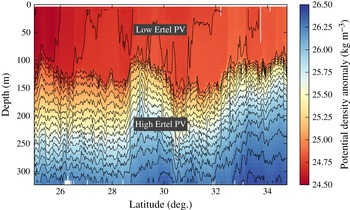
The upper ocean does not have a nearly constant PV, however, contrary to what is assumed in surface QG turbulence. Instead, a weakly-stratified mixed layer typically overlies a strongly-stratified thermocline (figure 1). There is a sharp step-like increase in stratification at the base of the mixed layer, corresponding to a step-like increase in background PV. This PV jump is dynamically important, because it supports edge waves that have the potential to interact with surface edge waves and thus produce a baroclinic instability in the mixed layer (e.g. Haine & Marshall Reference Haine and Marshall1998). This linear instability is to leading order captured by an Eady model with a rigid interface at the base of the mixed layer (Eady Reference Eady1949). Corrections due to ageostrophic effects and a moveable interface at the mixed-layer base can be computed (Stone Reference Stone1966b ; Boccaletti et al. Reference Boccaletti, Ferrari and Fox-Kemper2007), but for typical wintertime conditions, the instability scale and growth rate are qualitatively captured by Eady’s QG model. When baroclinic mixed-layer instabilities grow to finite amplitude, turbulent scale interactions distribute energy across scales. Because of the rotational constraint, they transfer energy preferentially to larger scales. This nonlinear dynamics has been studied in idealized mixed-layer models, where baroclinic mixed-layer instabilities grow on a prescribed front (e.g. Boccaletti et al. Reference Boccaletti, Ferrari and Fox-Kemper2007; Fox-Kemper, Ferrari & Hallberg Reference Fox-Kemper, Ferrari and Hallberg2008).
Potential temperature section from the wintertime eastern subtropical North Pacific. The data were obtained using a conductivity–temperature–depth sensor towed on a sawtooth profile along
 $140^{\circ }\,\text{W}$
as part of the Spice experiment on 28 January–2 February, 1997. For more information on the data, see Ferrari & Rudnick (Reference Ferrari and Rudnick2000).

In the real ocean, baroclinic mixed-layer instabilities occur in the presence of an energetic mesoscale eddy field, so mixed-layer modes can grow on mesoscale buoyancy gradients and can be sheared by mesoscale strain fields. Realistic submesoscale-permitting models capture this dynamics (e.g. Mensa et al. Reference Mensa, Garraffo, Griffa, Özgökmen, Haza and Veneziani2013; Sasaki et al. Reference Sasaki, Klein, Qiu and Sasai2014), but the models’ complexity makes it hard to distil the essence of the dynamics and even these simulations only marginally resolve many submesoscale phenomena. In this article, we explore submesoscale dynamics by formulating a QG model that allows both mixed layer and thermocline instabilities. This simple model of submesoscale turbulence energized by baroclinic mixed-layer instabilities captures salient features of wintertime observations of submesoscale flows. If the mixed layer in this model is eliminated, the submesoscale dynamics reverts to surface QG turbulence, which allows a straightforward comparison of the two mechanisms that can energize submesoscale turbulence.
We use QG scaling to formulate the dynamics of the model, which requires small Rossby and Froude numbers (e.g. Pedlosky Reference Pedlosky1987). Typical mesoscale Rossby and Froude numbers are on the order
 $0.1$
and increase slowly with wavenumber if the submesoscales are energetic, reaching order 1 at scales of order 1 km (Callies et al.
Reference Callies, Ferrari, Klymak and Gula2015). While the QG approximation does not apply anymore at these small scales, the QG system can be expected to capture the leading-order dynamics over the 10–100 km range.
A major limitation of QG dynamics in representing mixed-layer instabilities is that QG scaling does not allow for restratification. The weak mixed-layer stratification will be fixed in our QG model, whereas in reality there is a competition between restratification and atmospherically forced mixed-layer turbulence, which tends to keep the mixed layer deep and unstratified. The assumption is that the slower balanced dynamics described by the QG model develops on top of this background state, which is maintained by fast small-scale turbulence. A full description of mixed-layer dynamics will eventually need to consider the interplay of the fast and slow dynamics, a topic we hope to address in a future study (cf. Hamlington et al. Reference Hamlington, Van Roekel, Fox-Kemper, Julien and Chini2014). We take up the discussion of how other non-QG effects may alter the dynamics toward the end of the article.
As described above, our inquiry into the dynamics of a weakly-stratified mixed layer coupled to a strongly-stratified thermocline is motivated by the study of the submesoscale upper ocean. The model we present and the dynamics we describe, however, have relevance for the atmosphere as well, where a weakly-stratified troposphere is capped by a strongly-stratified stratosphere (e.g. Eady Reference Eady1949). The dynamics may also apply to the atmospheres of gas giants (e.g. Seiff et al. Reference Seiff, Kirk, Knight, Young, Mihalov, Young, Milos, Schubert, Blanchard and Atkinson1998) or other geophysical fluids that have layers of different stratification.
We formulate the model and give some physical intuition for its behaviour in § 2. In § 3, we investigate the linear dynamics of the model to understand its stability properties. This linear dynamics is suggestive of the fully-nonlinear turbulent dynamics that we address in § 4, where we analyse the energy spectra and fluxes for cases with and without baroclinic mixed-layer instabilities. We compare the results to observations in § 5 and conclude in § 6.
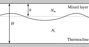
Schematic of the model set-up in a vertical–horizontal plane. There are rigid surfaces at
 $z=0$
and
 $z=-H$
and a deformable interface at the mean depth
 $z=-h$
, separating layers of constant stratification,
 $N_{m}$
in the mixed layer and
 $N_{t}$
in the thermocline.

2. Model formulation
Consider two layers with constant stratification and constant mean shear on an
 $f$
-plane, so that each layer has constant PV (figure 2). The upper layer represents the mixed layer, which has a mean depth
 $h$
, stratification
 $N_{m}$
, and mean zonal shear
 ${\it\Lambda}_{m}$
that is in thermal wind balance with the mean meridional buoyancy gradient
 $-f{\it\Lambda}_{m}$
. The lower layer represents the thermocline and has stratification
 $N_{t}$
and mean zonal shear
 ${\it\Lambda}_{t}$
that is in thermal wind balance with the mean meridional buoyancy gradient
 $-f{\it\Lambda}_{t}$
. The total depth is
 $H$
. The layers are coupled through a deformable interface; flat rigid boundaries are assumed at both the surface and the bottom. The presence of a rigid bottom at the base of the thermocline is not realistic, but we will show that the bottom layer still captures the key thermocline physics relevant to our study. A weakly-stratified abyssal layer could be included but is omitted for simplicity, because it does not significantly affect the surface submesoscale dynamics of interest here. The approximation that the stratification is discontinuous at the base of the mixed layer is appropriate at horizontal scales larger than the deformation radius
 $Nd/f$
associated with the transition depth
 $d$
between the mixed layer and the thermocline (Smith & Bernard Reference Smith and Bernard2013). The transition at the base of the mixed layer is typically quite sharp (figure 1), so this deformation radius is much smaller than the submesoscales we are interested in here.
The assumption of a uniform PV within the two layers greatly simplifies the dynamics. PV conservation within the layers is trivial, as in the classic Eady (Reference Eady1949) problem. The flow in the interior of the layers is obtained by solving (1.1), with the boundary conditions supplied by the distribution of buoyancy at the surface and bottom and by matching conditions at the interface between the mixed layer and the thermocline.
In QG, the buoyancy anomaly
 $b$
is governed by the horizontal advection of buoyancy anomalies by the geostrophic flow and by the vertical advection of the background buoyancy field,
 $$\begin{eqnarray}\frac{\partial b}{\partial t}+\text{J}({\it\psi},b)+wN^{2}=0.\end{eqnarray}$$
At the surface and bottom, where the vertical velocity
 $w$
vanishes, buoyancy anomalies are conserved under horizontal advection and (2.1) reduces to (1.2). To ensure that pressure is continuous at the interface, we require that the streamfunction
 ${\it\psi}$
is continuous. Mass conservation requires that the vertical velocity
 $w$
also is continuous. These conditions are applied at
 $z=-h$
, consistent with QG scaling. The conservation equations for buoyancy just above the interface at
 $z=-h$
,
 $$\begin{eqnarray}\frac{\partial b^{+}}{\partial t}+\text{J}({\it\psi}_{1},b^{+})+wN_{m}^{2}=0,\quad b^{+}=f\frac{\partial {\it\psi}}{\partial z}(-h^{+}),\end{eqnarray}$$
and just below the interface,
 $$\begin{eqnarray}\frac{\partial b^{-}}{\partial t}+\text{J}({\it\psi}_{1},b^{-})+wN_{t}^{2}=0,\quad b^{-}=f\frac{\partial {\it\psi}}{\partial z}(-h^{-}),\end{eqnarray}$$
can then be combined to eliminate
 $w$
, where
 ${\it\psi}_{1}$
denotes the streamfunction at
 $z=-h$
. This gives a conservation law for the quantity
 $$\begin{eqnarray}{\it\theta}_{1}=f\left(\frac{b^{+}}{N_{m}^{2}}-\frac{b^{-}}{N_{t}^{2}}\right),\end{eqnarray}$$
which is simply advected by the horizontal flow at the interface,
 $$\begin{eqnarray}\frac{\partial {\it\theta}_{1}}{\partial t}+\text{J}({\it\psi}_{1},{\it\theta}_{1})=0.\end{eqnarray}$$
It should be noted that this does not ensure that buoyancy is continuous at
 $z=-h$
. Instead, there is an implied interface displacement and buoyancy is continuous across the displaced interface. The displacement is small and, consistent with QG scaling, the matching conditions are applied at
 $z=-h$
.
The quantity
 ${\it\theta}_{1}$
is nothing but the integrated PV associated with the interface displacement, as can be verified by integrating
 $$\begin{eqnarray}q={\rm\nabla}^{2}{\it\psi}+f\frac{\partial }{\partial z}\left(\frac{b}{N^{2}}\right)\end{eqnarray}$$
across the interface. (The relative vorticity term vanishes because
 ${\it\psi}$
is continuous across the interface.) While there are no PV anomalies within the two layers, the displacement of the interface between the layers induces a PV anomaly that, according to (2.5) and consistent with QG dynamics, is advected by the geostrophic flow at
 $z=-h$
. The conservation equation (2.5) has been used to study the dynamics of the tropopause, which is similarly an interface between the weakly stratified fluid in the troposphere and the strongly stratified fluid in the stratosphere (Eady Reference Eady1949; Rivest, Davis & Farrell Reference Rivest, Davis and Farrell1992; Juckes Reference Juckes1994; Held et al.
Reference Held, Pierrehumbert, Garner and Swanson1995).
The two-layer model can equivalently be interpreted as consisting of three PV sheets:
 $$\begin{eqnarray}q={\it\theta}_{0}{\it\delta}(z)+{\it\theta}_{1}{\it\delta}(z+h)+{\it\theta}_{2}{\it\delta}(z+H),\end{eqnarray}$$
where
 ${\it\delta}$
is Dirac’s delta function and
 ${\it\theta}_{0}=-fb/N_{m}^{2}$
at
 $z=0$
,
 ${\it\theta}_{2}=fb/N_{t}^{2}$
at
 $z=-H$
and
 ${\it\theta}_{1}$
at
 $z=-h$
is given in (2.4). PV is advected by the geostrophic flow, so
 $$\begin{eqnarray}\frac{\partial {\it\theta}_{j}}{\partial t}+\text{J}({\it\psi}_{j},{\it\theta}_{j})=0,\end{eqnarray}$$
where
 $j=0,1,2$
and
 ${\it\psi}_{j}$
is the streamfunction at the level corresponding to
 ${\it\theta}_{j}$
. This formulation is simply an extension of Bretherton’s (Reference Bretherton1966) representation of boundary conditions to include an interior PV sheet due to the deflection of an interface between layers of different stratification.
Note that even though
 ${\it\theta}_{1}$
is only advected by the geostrophic flow, this does not imply that
 $w=0$
at the interface, much like the fact that interior PV anomalies in the QG system are only advected by the geostrophic flow does not imply that
 $w=0$
. The vertical velocity is implicit in the dynamics and can be solved for using the omega equation (e.g. Hoskins et al.
Reference Hoskins, Draghici and Davies1978).
To complete the dynamics, we require an inversion relation that allows us to obtain the streamfunctions
 ${\it\psi}_{j}$
from the conserved quantities
 ${\it\theta}_{j}$
. For simplicity, we consider a doubly-periodic domain and express the inversion relation as a linear equation for Fourier coefficients of the variables
 ${\it\theta}_{j}$
and
 ${\it\psi}_{j}$
:
 $$\begin{eqnarray}\hat{{\bf\theta}}=\unicode[STIX]{x1D647}\hat{{\bf\psi}},\quad {\bf\theta}=({\it\theta}_{0},{\it\theta}_{1},{\it\theta}_{2})^{\text{T}},\quad {\bf\psi}=({\it\psi}_{0},{\it\psi}_{1},{\it\psi}_{2})^{\text{T}}.\end{eqnarray}$$
where Fourier transforms are denoted by carets. The matrix
 $\unicode[STIX]{x1D647}$
, which depends on the zonal and meridional wavenumbers
 $k$
and
 $l$
, is determined by solving
 $$\begin{eqnarray}-\!{k_{h}}^{2}\hat{{\it\psi}}+\frac{\partial }{\partial z}\left(\frac{f^{2}}{N^{2}}\frac{\partial \hat{{\it\psi}}}{\partial z}\right)=0\end{eqnarray}$$
in each layer, where
 $k_{h}=(k^{2}+l^{2})^{1/2}$
is the magnitude of the horizontal wavenumber vector. The first column of
 $\unicode[STIX]{x1D647}$
is determined by setting
 $\hat{{\bf\psi}}=(1,0,0)^{\text{T}}$
, solving (2.10) for
 $\hat{{\it\psi}}(z)$
and subsequently calculating
 ${\it\theta}_{0}$
,
 ${\it\theta}_{1}$
and
 ${\it\theta}_{2}$
. Repeating for
 $\hat{{\bf\psi}}=(0,1,0)^{\text{T}}$
and
 $\hat{{\bf\psi}}=(0,0,1)^{\text{T}}$
gives
 $$\begin{eqnarray}\unicode[STIX]{x1D647}=fk_{h}\left(\begin{array}{@{}ccc@{}}\displaystyle -\frac{\coth {\it\mu}_{m}}{N_{m}} & \displaystyle \frac{\text{csch}\,{\it\mu}_{m}}{N_{m}} & 0\\ \displaystyle \frac{\text{csch}\,{\it\mu}_{m}}{N_{m}} & \displaystyle -\frac{\coth {\it\mu}_{m}}{N_{m}}-\frac{\coth {\it\mu}_{t}}{N_{t}} & \displaystyle \frac{\text{csch}\,{\it\mu}_{t}}{N_{t}}\\ \displaystyle 0 & \displaystyle \frac{\text{csch}\,{\it\mu}_{t}}{N_{t}} & \displaystyle -\frac{\coth {\it\mu}_{t}}{N_{t}}\end{array}\right),\end{eqnarray}$$
where
 ${\it\mu}_{m}=N_{m}k_{h}h/f$
and
 ${\it\mu}_{t}=N_{t}k_{h}(H-h)/f$
are non-dimensional wavenumbers. This
 $3\times 3$
matrix can easily be inverted.
This model can be generalized to an arbitrary number of layers of constant stratification and shear, which may be a useful way to approximate more realistic stratification and shear profiles. This is discussed in appendix A. The model can also be extended to include a density jump at the interface, as is sometimes present at the base of the mixed layer. The formulation is given in appendix B. Here we consider only the case of a continuous density profile, which is simpler and captures the essential physics of the submesoscale ocean.
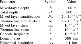
Parameters used throughout this article unless otherwise noted. These are typical of the wintertime midlatitude ocean.
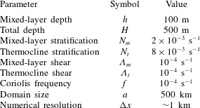
To build intuition for the dynamics of the model, we illustrate the vertical structure of the flow associated with anomalies of
 ${\it\theta}_{j}$
at the surface, the interface and the bottom. Here and throughout the article, we use the parameters given in table 1, which are typical of the wintertime midlatitude ocean. (The values listed imply a mixed-layer Richardson number of
 $N_{m}^{2}/{\it\Lambda}_{m}^{2}=400$
, which is larger than the order-1 Richardson numbers typically considered (e.g. Boccaletti et al.
Reference Boccaletti, Ferrari and Fox-Kemper2007). The relatively large Richardson number is the result of a relatively weak shear, which is chosen such that realistic energy levels are reached in the nonlinear simulations described below. QG dynamics overestimates the baroclinic growth rate for small Richardson numbers (Stone Reference Stone1966b
), which would result in unrealistically strong mixed-layer instabilities if a larger shear was chosen. It should also be noted that the leading-order QG dynamics can be rescaled to different Richardson numbers.) At the largest scales, for
 ${\it\theta}_{j}$
anomalies with wavelength
 ${\it\lambda}=1000~\text{km}$
or
 $k_{h}\ll f/N_{t}H$
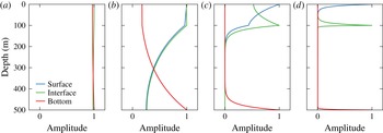
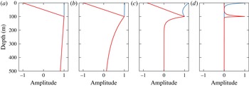
, the flow is nearly depth independent, irrespective of which level the anomaly is at (figure 3
a). Around the thermocline deformation radius, at
 ${\it\lambda}=100~\text{km}$
or
 $k_{h}\sim f/N_{t}H\ll f/N_{m}h$
, flow anomalies significantly decay in the thermocline, while the flow is nearly uniform across the mixed layer (figure 3
b). Surface (
 ${\it\theta}_{0}$
) and interface (
 ${\it\theta}_{1}$
) anomalies still induce significant flow at the bottom and vice versa. Around the mixed-layer deformation radius, at
 ${\it\lambda}=10~\text{km}$
or
 $k_{h}\sim f/N_{m}h\gg f/N_{t}H$
, surface (
 ${\it\theta}_{0}$
) and interface (
 ${\it\theta}_{1}$
) anomalies induce very little flow at the bottom and vice versa (figure 3
c). The flow now varies significantly across the mixed layer, but surface anomalies (
 ${\it\theta}_{0}$
) still induce significant flow at the interface and vice versa. At
 ${\it\lambda}=1~\text{km}$
or
 $k_{h}\gg f/N_{m}h$
, all levels are decoupled:
 ${\it\theta}_{j}$
anomalies on any one of the levels induce very little flow at the other levels (figure 3
d).
Vertical structure of streamfunction amplitude associated with anomalies of
 ${\it\theta}_{0}$
(surface),
 ${\it\theta}_{1}$
(interface) and
 ${\it\theta}_{2}$
(bottom). Shown are the vertical profiles for
 ${\it\theta}_{j}$
anomalies with different horizontal wavenumbers
 $k_{h}=2{\rm\pi}/{\it\lambda}$
. The wavelength
 ${\it\lambda}$
is given in the respective panel title: (a) 1000 km wavelength; (b) 100 km wavelength; (c) 10 km wavelength; (d) 1 km wavelength.

The dependence of the vertical flow structure on the horizontal scale of the anomalies illuminates the qualitative dynamics of the model. At the largest scales, the flow is essentially depth independent and follows two-dimensional dynamics. At scales
 $k_{h}\sim f/N_{t}H$
, around the thermocline deformation radius, surface or interface anomalies can interact with bottom anomalies, allowing phase locking and a thermocline instability. At scales
 $k_{h}\sim f/N_{m}h$
, around the mixed-layer deformation radius, surface and interface anomalies can interact, enabling an instability in the mixed layer. Bottom anomalies, on the other hand, are decoupled, so there is no thermocline instability at these scales. At the smallest scales, all three levels are independent and follow surface QG dynamics.
3. Linear stability analysis
We now analyse the linear stability of the model formulated above. This linear analysis reveals the nature of the instabilities that fuel the nonlinear turbulence, which we describe in the next section.
Blumen (Reference Blumen1979) analysed short-wave instabilities in the atmosphere using a model consisting of two coupled constant-PV layers. He performed a linear stability analysis equivalent to what will be presented here. For completeness, we repeat the analysis in the context of upper ocean dynamics to emphasize the aspects most relevant for the nonlinear regime.
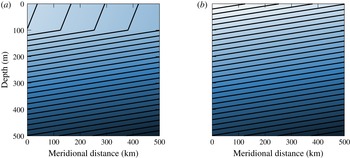
Mean buoyancy structure in the meridional–vertical plane for (a) the full model and (b) the thermocline-only model. The contours show isopycnals; light shading indicates more buoyant fluid.

We consider the linear stability of normal-mode perturbations to a zonal flow with constant vertical shear
 ${\it\Lambda}_{m}$
in the mixed layer and
 ${\it\Lambda}_{t}$
in the thermocline (figure 4). The linearized conservation equation for the perturbations from this mean state, written in Fourier space, is
 $$\begin{eqnarray}\frac{\partial \hat{{\bf\theta}}}{\partial t}+\text{i}k\unicode[STIX]{x1D650}\hat{{\bf\theta}}+\text{i}k{\it\bf\Gamma}\hat{{\bf\psi}}=0,\end{eqnarray}$$
where the mean zonal flows and mean meridional PV gradients at the respective levels are represented by the diagonal elements of the matrices
 $\unicode[STIX]{x1D650}$
and
 ${\it\bf\Gamma}$
:
 $$\begin{eqnarray}\displaystyle & \unicode[STIX]{x1D650}=\text{diag}(0,-{\it\Lambda}_{m}h,-{\it\Lambda}_{m}h-{\it\Lambda}_{t}(H-h)), & \displaystyle\end{eqnarray}$$
 $$\begin{eqnarray}\displaystyle & {\it\bf\Gamma}=\text{diag}(f^{2}{\it\Lambda}_{m}/N_{m}^{2},-f^{2}{\it\Lambda}_{m}/N_{m}^{2}+f^{2}{\it\Lambda}_{t}/N_{t}^{2},-f^{2}{\it\Lambda}_{t}/N_{t}^{2}). & \displaystyle\end{eqnarray}$$
 $\hat{{\bf\psi}}$
and obtain an equation for the
 $\hat{{\bf\theta}}$
coefficients only,
 $$\begin{eqnarray}\frac{\partial \hat{{\bf\theta}}}{\partial t}+\text{i}k\unicode[STIX]{x1D650}\hat{{\bf\theta}}+\text{i}k{\it\bf\Gamma}\unicode[STIX]{x1D647}^{-1}\hat{{\bf\theta}}=0.\end{eqnarray}$$
Substituting
 $\hat{{\bf\theta}}=\tilde{{\bf\theta}}\text{e}^{-\text{i}{\it\omega}t}$
, with complex frequency
 ${\it\omega}$
, turns this equation for
 $\hat{{\bf\theta}}$
into the eigenvalue problem
 $$\begin{eqnarray}(\unicode[STIX]{x1D650}+{\it\bf\Gamma}\unicode[STIX]{x1D647}^{-1})\tilde{{\bf\theta}}=c\tilde{{\bf\theta}},\end{eqnarray}$$
where the eigenvalue is
 $c={\it\omega}/k$
. The real part of
 $c$
is the zonal phase speed; the imaginary part gives the growth rate
 ${\it\sigma}=k\,\text{Im}c$
.
Being a third-order system, (3.5) can be solved analytically, but the solutions are rather complicated and give little useful insight. We instead explore the characteristics of the solutions numerically for the set of parameters given in table 1. We then explain the stability properties and parameter dependencies by considering special limit cases.
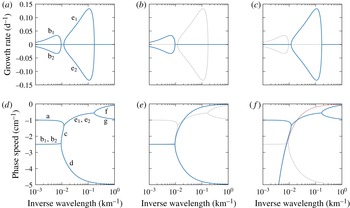
Linear stability analysis of the model equations. (a) Growth rates and (d) phase speeds of the full model, (b) growth rates and (e) phase speeds of the thermocline-only model, (c) growth rates and (f) phase speeds of the mixed-layer-only model. Growth rates and phase speeds are shown in blue; the growth rates and phase speeds of the full model are overlaid for reference in grey. The phase speed of a surface edge wave is given in faint red in (f).

3.1. Full model
We start by considering the growth rate
 ${\it\sigma}$
as a function of horizontal wavenumber. The eigenvalue problem (3.5) only depends on
 $k_{h}=(k^{2}+l^{2})^{1/2}$
, so the eigenvalue
 $c$
is a function of
 $k_{h}$
only. For a given
 $k_{h}$
, the maximum growth rate
 ${\it\sigma}=k\,\text{Im}c$
hence occurs at
 $l=0$
. We therefore only consider disturbances with no meridional dependence.
Plotting the growth rate
 ${\it\sigma}$
as a function of zonal wavenumber
 $k$
reveals that there are two lobes of instability: one at the mesoscale and one at the submesoscale (figure 5
a, branches ‘b’ and ‘e’). The maximum growth rates occur at zonal wavelengths of approximately 160 km (mesoscale) and 9 km (submesoscale). The two lobes can overlap, for example if the mixed layer is deeper or if a density jump at the base of the mixed layer is included (not shown). The submesoscale instability has a peak growth rate much larger than the mesoscale instability. The growth rates are similar to what Boccaletti et al. (Reference Boccaletti, Ferrari and Fox-Kemper2007) found in a linear QG stability analysis of a realistic mean state of the wintertime eastern subtropical North Pacific. The magnitudes are slightly smaller here, because the shear is slightly weaker. But the similarity of the instabilities supports that this model, despite being highly idealized, captures the essential physics of mesoscale and submesoscale instabilities. Whether it also captures the essential physics in the nonlinear regime will be discussed in §§ 4–6.
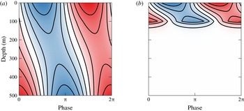
The mesoscale and submesoscale instabilities have very different vertical structures, as also noted by Boccaletti et al. (Reference Boccaletti, Ferrari and Fox-Kemper2007). The perturbation streamfunctions – derived from the eigenvectors of (3.5) – show that the fastest-growing mesoscale mode is deep and spans the entire water column (figure 6 a), whereas the fastest-growing submesoscale mode is almost completely confined to the mixed layer, with only weak penetration into the thermocline below 100 m depth (figure 6 b). Both modes exhibit the familiar pattern of baroclinically unstable modes with streamfunction perturbations tilted into the shear, as is necessary to extract potential energy from the mean flow.
Further insight into the dynamics of the model can be gained by considering the propagation speeds of the linear modes in conjunction with their growth rates (figure 5 a,d). Being a third-order system, the model has three normal modes at each wavenumber. In both lobes of instability, the growing modes are conjugate to decaying modes, which have the same phase speeds. This is the familiar phase locking of counter-propagating waves in baroclinic instability (branches ‘b’ and ‘e’). In these unstable wavenumber ranges, there is an additional neutral mode (branches ‘a’ and ‘d’). At wavenumbers with no instability, all three modes have distinct phase speeds – no phase locking occurs. We will discuss the dynamics of the various branches by considering approximations to the full model.
Perturbation streamfunction of the most unstable (a) mesoscale (160 km) and (b) submesoscale (9 km) modes of the full model. Red and blue shading represents positive and negative values, respectively.

3.2. Thermocline only
We start by examining the deep mesoscale instability of the full model. As discussed in the model formulation (§ 2), the mesoscale modes are deep and only slightly modified by the presence of the mixed layer. We can understand the mesoscale instability by eliminating the mixed layer altogether and considering a thermocline-only model (figure 4
b). This amounts to setting
 $h=0$
(or
 $N_{m}=N_{t}$
and
 ${\it\Lambda}_{m}={\it\Lambda}_{t}$
) in the full model. In this limit, the model reduces to one layer with the dynamics controlled by buoyancy advection at the surface and bottom only – the classic Eady (Reference Eady1949) model. The inversion matrix (2.11) reduces to
 $$\begin{eqnarray}\unicode[STIX]{x1D647}=fk_{h}\left(\begin{array}{@{}cc@{}}\displaystyle -\frac{\coth {\it\mu}_{t}}{N_{t}} & \displaystyle \frac{\text{csch}\,{\it\mu}_{t}}{N_{t}}\\ \displaystyle \frac{\text{csch}\,{\it\mu}_{t}}{N_{t}} & \displaystyle -\frac{\coth {\it\mu}_{t}}{N_{t}}\end{array}\right),\end{eqnarray}$$
and the matrices representing the mean flow are
 $$\begin{eqnarray}\displaystyle & \unicode[STIX]{x1D650}=\text{diag}(0,-{\it\Lambda}_{t}H), & \displaystyle\end{eqnarray}$$
 $$\begin{eqnarray}\displaystyle & {\it\bf\Gamma}=\text{diag}(f^{2}{\it\Lambda}_{t}/N_{t}^{2},-f^{2}{\it\Lambda}_{t}/N_{t}^{2}). & \displaystyle\end{eqnarray}$$
 $$\begin{eqnarray}c=-\frac{{\it\Lambda}_{t}H}{2}\pm \frac{\text{i}{\it\Lambda}_{t}H}{{\it\mu}_{m}}\left({\it\mu}_{t}\coth {\it\mu}_{t}-1-\frac{{\it\mu}_{t}^{2}}{4}\right)^{1/2},\end{eqnarray}$$
where
 ${\it\mu}_{t}=N_{t}k_{h}H/f$
is the non-dimensional wavenumber (Eady Reference Eady1949).
The solution (3.9) shows that this thermocline-only model has a baroclinic instability near the thermocline deformation radius
 $N_{t}H/f$
. The maximum growth rate
 ${\it\sigma}=0.31f{\it\Lambda}_{t}/N_{t}$
occurs at
 ${\it\mu}_{t}=1.6$
and
 $l=0$
, which corresponds to a zonal wavelength
 ${\it\lambda}=3.9N_{t}H/f$
. The growth curve for this thermocline-only model approximates the mesoscale lobe of the full model very well (figure 5
b). The short-wave cutoff in the Eady model at
 ${\it\lambda}=2.6N_{t}H/f$
nearly coincides with the short-wave cutoff of the mesoscale instability in the full model. The phase speed of the phase-locked waves
 $-{\it\Lambda}_{t}H/2$
very nearly matches the phase speed of the unstable mesoscale mode of the full model (figure 5
e). The split at the short-wave cutoff into surface and bottom modes also features in the full model. In the thermocline-only model, these surface and bottom modes are very nearly Eady edge waves that do not sense the other boundary. The bottom mode of the thermocline-only model very nearly matches that of the full model (branch ‘d’). The surface mode of the thermocline-only model traces out branch ‘c’ of the full model, but then the full model transitions to dynamics associated with the mixed layer that are not present in the thermocline-only model.
This comparison shows that the mesoscale instability of the full model very nearly follows Eady dynamics. The presence of the mixed layer only modifies the characteristics of the instability slightly. At submesoscales, on the other hand, the thermocline-only model has surface QG dynamics, as opposed to the mixed-layer dynamics of the full model.
3.3. Mixed layer only
Turning our attention to the submesoscale instability, we note that the submesoscale instability peaks around the deformation radius of the mixed layer
 $N_{m}h/f$
. Based on the discussion in the model formulation (§ 2) and the vertical structure of this instability (figure 6
b), we anticipate that this instability arises from the interaction between anomalies at the surface and at the interface between mixed layer and thermocline.
In a first attempt to isolate the submesoscale instability, we disregard the possibility that surface and interface anomalies induce flow in the thermocline and assume a rigid bottom at the base of the mixed layer. This reduces the full model to an Eady model for the mixed layer, which is the limit of infinite thermocline stratification. This Eady model reasonably approximates the location and magnitude of the peak growth rate with
 ${\it\lambda}=3.9N_{m}h/f=8~\text{km}$
and
 ${\it\sigma}=0.31f{\it\Lambda}_{m}/N_{m}=0.13~\text{d}^{-1}$
. The Eady model captures the short-wave cutoff of the full model, but misses the long-wave cutoff. This suggests that the fastest-growing mode approximately follows Eady dynamics as if the thermocline acted like a rigid bottom, but also that larger-scale modes are significantly modified by reaching into the thermocline.
All features of the submesoscale instability are captured if flow in the thermocline is allowed. To still isolate the submesoscale instability, we consider again the layered model but let the thermocline be infinitely deep. That eliminates bottom edge waves, so no mesoscale instability occurs. Eady (Reference Eady1949) considered the upside-down atmospheric analogue to this system, relaxing the assumption that a rigid lid is placed at the tropopause.
Our system with no bottom again reduces to two variables; the inversion matrix is
 $$\begin{eqnarray}\unicode[STIX]{x1D647}=fk_{h}\left(\begin{array}{@{}cc@{}}\displaystyle -\frac{\coth {\it\mu}_{m}}{N_{m}} & \displaystyle \frac{\text{csch}\,{\it\mu}_{m}}{N_{m}}\\ \displaystyle \frac{\text{csch}\,{\it\mu}_{m}}{N_{m}} & \displaystyle -\frac{\coth {\it\mu}_{m}}{N_{m}}-\frac{1}{N_{t}}\end{array}\right)\end{eqnarray}$$
and the mean flow is represented by
 $$\begin{eqnarray}\displaystyle & \unicode[STIX]{x1D650}=\text{diag}(0,-{\it\Lambda}_{m}h), & \displaystyle\end{eqnarray}$$
 $$\begin{eqnarray}\displaystyle & {\it\bf\Gamma}=\text{diag}(f^{2}{\it\Lambda}_{m}/N_{m}^{2},-f^{2}{\it\Lambda}_{m}/N_{m}^{2}+f^{2}{\it\Lambda}_{t}/N_{t}^{2}). & \displaystyle\end{eqnarray}$$
 ${\it\Lambda}={\it\Lambda}_{m}={\it\Lambda}_{t}$
, the solution to the eigenvalue problem (3.5) is
 $$\begin{eqnarray}c=-\frac{{\it\Lambda}h}{2}\left(1+\frac{{\it\alpha}}{{\it\mu}_{m}}\right)\pm \frac{\text{i}{\it\Lambda}h}{{\it\mu}_{m}}\left[\frac{(1-{\it\alpha}^{2})({\it\mu}_{m}-\tanh {\it\mu}_{m})}{\tanh {\it\mu}_{m}+{\it\alpha}}-\frac{1}{4}({\it\mu}_{m}-{\it\alpha})^{2}\right]^{1/2},\end{eqnarray}$$
where
 ${\it\alpha}=N_{m}/N_{t}$
(Eady Reference Eady1949; Blumen Reference Blumen1979). This converges to the classic Eady solution if
 ${\it\alpha}\ll 1$
and
 ${\it\alpha}\ll {\it\mu}_{m}$
, which is equivalent to
 $N_{t}\gg N_{m}$
and
 $k_{h}\gg f/N_{t}h$
. This shows that large thermocline stratification acts like a rigid bottom, but only for scales that are not too large, as alluded to above. Modes of large horizontal scale penetrate into the thermocline and their dynamics is altered.
The growth rates and phase speeds of this reduced model very nearly match the growth rates and phase speeds of the full model at scales smaller than about 100 km (figure 5
c,f). This model now captures the long-wave cutoff of the submesoscale instability. At large scales, where
 ${\it\mu}_{m}\ll {\it\alpha}$
and
 ${\it\mu}_{m}\ll 1$
or equivalently
 $k_{h}\ll f/N_{t}h$
and
 $k_{h}\ll f/N_{m}h$
, the dynamics split into modes that are barotropic and baroclinic in the mixed layer. The barotropic mode behaves like a surface edge wave, which has a phase speed
 $-f{\it\Lambda}/N_{t}k_{h}$
and does not sense the mixed layer (figure 5
f). The baroclinic mode is baroclinic in the mixed layer and remains shallow for large scales – its critical level is the base of the mixed layer and its phase speed is
 $-{\it\Lambda}h$
. The vastly different phase speeds of these two modes prevent phase locking, so no instability occurs at large scales. This stabilization is analogous to that by the
 ${\it\beta}$
-effect (Phillips Reference Phillips1954; Lindzen Reference Lindzen1994; Vallis Reference Vallis2006). Note that no tilt in the interface is required for this long-wave cutoff (cf. Boccaletti et al.
Reference Boccaletti, Ferrari and Fox-Kemper2007). For the unstable modes, the reduced model with no bottom also captures the deepening of the critical level as the scale increases,
 $-{\it\Lambda}h(1+f/N_{t}k_{h}h)/2$
, which is due to the increasing penetration of the unstable mode into the thermocline.
The location of the long-wave cutoff in this constant-shear case depends on the ratio
 $N_{m}/N_{t}$
. In the more general case
 ${\it\Lambda}_{m}\neq {\it\Lambda}_{t}$
, it also depends on the ratio
 ${\it\Lambda}_{m}/{\it\Lambda}_{t}$
. No long-wave cutoff occurs if
 ${\it\Lambda}_{t}=0$
, as found by Rivest et al. (Reference Rivest, Davis and Farrell1992), who considered the atmospheric case with no shear in the stratosphere. There is also no long-wave cutoff if
 $N_{m}/N_{t}\rightarrow 0$
, which is the Eady limit. The instability itself requires a reversal of the PV gradient, so the condition for instability is
 ${\it\Lambda}_{m}/N_{m}^{2}>{\it\Lambda}_{t}/N_{t}^{2}$
. This condition is typically satisfied in the ocean, because the thermocline stratification is much larger than the mixed-layer stratification and horizontal buoyancy gradients are typically of the same order in the mixed layer as in the thermocline, if not larger.
3.4. Summary
We are now in a position to understand all branches in the phase speed diagram of the full model. Branch ‘a’ is a mode that is baroclinic in the mixed layer and does not penetrate much into the thermocline. It does not sense the bottom. Branch ‘
 $\text{b}_{1}$
’ is the unstable branch corresponding to the Eady-like thermocline instability; branch ‘
 $\text{b}_{2}$
’ is the conjugate decaying branch. Branch ‘c’ is a mode that is nearly barotropic in the mixed layer and behaves like a surface edge wave in the thermocline. It does not interact much with the bottom. Branch ‘d’ is a bottom edge wave that is independent of the surface and interface. Branch ‘
 $\text{e}_{1}$
’ is the unstable branch corresponding to the mixed-layer instability; branch ‘
 $\text{e}_{2}$
’ is the conjugate decaying branch. The instability is significantly modified by the modes’ penetration into the thermocline, but the scale and growth rate of the most unstable mode still scale with the mixed-layer deformation radius and the Eady growth rate. Branches ‘f’ and ‘g’ are edge waves propagating on the surface and the interface that do not interact with any of the other edge waves.
4. Nonlinear dynamics
We now turn to the nonlinear dynamics that arises when perturbations are amplified by the instabilities and grow to finite amplitude. We solve numerically the full nonlinear equations
 $$\begin{eqnarray}\frac{\partial {\bf\theta}}{\partial t}+\unicode[STIX]{x1D650}\frac{\partial {\bf\theta}}{\partial x}+{\it\bf\Gamma}\frac{\partial {\bf\psi}}{\partial x}+\text{J}({\bf\psi},{\bf\theta})=r{\rm\nabla}^{-2}{\bf\theta}-{\it\nu}(-{\rm\nabla}^{2})^{n}{\bf\theta},\end{eqnarray}$$
where the Jacobian operator is understood to act element-wise:
 $$\begin{eqnarray}\text{J}({\bf\psi},{\bf\theta})=(\text{J}({\it\psi}_{0},{\it\theta}_{0}),\text{J}({\it\psi}_{1},{\it\theta}_{1}),\text{J}({\it\psi}_{2},{\it\theta}_{2}))^{\text{T}}.\end{eqnarray}$$
These are the evolution equations for perturbations from the prescribed mean zonal flow, which appears in form of the diagonal matrices
 $\unicode[STIX]{x1D650}$
and
 ${\it\bf\Gamma}$
. We consider flows that are doubly periodic in the perturbations, so no modification of the prescribed mean can occur. We introduce hypoviscosity with coefficient
 $r$
, which provides a drag to remove energy from large scales, and hyperviscosity with coefficient
 ${\it\nu}$
and order
 $n$
, which helps ensure numerical stability and absorbs enstrophy at small scales. Hypoviscosity is a convenient but somewhat unphysical choice. We introduce it to halt the inverse cascade and allow for mesoscale equilibration. Hypoviscosity appears in the dynamical equations for the conserved quantities at the surface, interface and bottom, but it can be thought of as acting throughout the layers. If applied to buoyancy and momentum, it does not affect PV and PV conservation within the layers remains trivial. Linear drag cannot prevent an inverse cascade to the domain scale without significantly damping the instabilities.
We integrate these equations on a
 $500~\text{km}\times 500~\text{km}$
domain using a fully dealiased pseudo-spectral code with a resolution
 $512\times 512$
. The time derivatives are discretized using a fourth-order Runge–Kutta scheme. The hypoviscosity coefficient is
 $r=10^{-16}~\text{m}^{-2}~\text{s}^{-1}$
; the hyperviscosity is of order
 $n=10$
and the coefficient is
 ${\it\nu}=2.5\times 10^{46}~\text{m}^{20}~\text{s}^{-1}$
. All calculations are initialized with white noise of small amplitude in
 ${\it\theta}_{j}$
.
Before considering the combined effect of mesoscale and mixed-layer instabilities, we first consider them separately. We start with the thermocline-only model, which allows only the mesoscale thermocline instability while submesoscale flows follow surface QG dynamics. We subsequently contrast this case with the mixed-layer-only model, which allows only the submesoscale mixed-layer instability. We finally consider the full model, in which both instabilities occur.
4.1. Thermocline only
We start by studying surface QG turbulence generated by mesoscale eddies, one of the proposed mechanisms to energize submesoscale flows. Surface QG flows cannot themselves extract energy from the mean flow, so they must be forced at the mesoscale. Instead of prescribing external forcing (e.g. Pierrehumbert, Held & Swanson Reference Pierrehumbert, Held and Swanson1994; Scott Reference Scott2006), we use the thermocline-only Eady model to generate mesoscale eddies that in turn generate the submesoscale flows. As we saw in the linear stability analysis, the dynamics of surface buoyancy anomalies in this model decouple from the bottom at scales smaller than the thermocline deformation radius, so flows very nearly follow surface QG dynamics at the submesoscales, i.e. the scales smaller than the thermocline deformation radius. The mesoscale instability is an obviously crude representation of the real mesoscale instability, with no interior PV gradients and the presence of an artificial rigid interface at the base of the thermocline. But the instability does generate mesoscale eddies of roughly the right scale, which is sufficient to drive the submesoscale surface QG flows (cf. Roullet et al. Reference Roullet, McWilliams, Capet and Molemaker2012).
Since the dissipative terms are weak in the linear regime, the instability grows until it reaches finite amplitude, when the nonlinear terms become important. Secondary instabilities set in and the flow quickly evolves into a fully turbulent regime. The perturbations grow in scale until they reach a scale where hypoviscosity is significant. Thereby, the flow comes into statistical equilibrium, which is the time period considered in what follows.
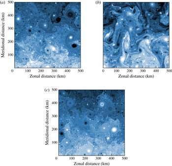
A snapshot from the equilibrated state exhibits a patchy surface buoyancy field with strong buoyancy gradients (figure 7 b). The largest eddies are about 200 km in scale. The strongest coherent vortices have a scale of about 50 km. Smaller-scale vortices are present, but are weaker the smaller the scale. They result from a roll-up instability that features prominently in the evolution of the flow (Held et al. Reference Held, Pierrehumbert, Garner and Swanson1995).
Snapshots of surface buoyancy (mean plus anomalies) from the equilibrated states of the (a) the full model, (b) the thermocline-only model, and (c) the mixed-layer-only model. The colour scale extends from white (more buoyant) through blue to black (less buoyant) and extends between
 $\pm f{\it\Lambda}a$
.

As typical for turbulent flows, a continuum of scales is energized. This is quantified by the kinetic and potential energy spectra in statistical equilibrium,
 $\langle K_{k,l}\rangle$
and
 $\langle P_{k,l}\rangle$
, which are defined by
 $$\begin{eqnarray}K_{k,l}=\frac{1}{2}(|\hat{u} |^{2}+|\hat{v}|^{2}),\quad P_{k,l}=\frac{1}{2}\frac{|\hat{b}|^{2}}{N^{2}}.\end{eqnarray}$$
The angle brackets denote an average in time, performed over the statistical equilibrium, and
 $u$
and
 $v$
denote the leading-order zonal and meridional geostrophic velocity components. Isotropic spectra
 $\langle K_{k_{h}}\rangle$
and
 $\langle P_{k_{h}}\rangle$
are computed by averaging
 $\langle K_{k,l}\rangle$
and
 $\langle P_{k,l}\rangle$
over circles of constant
 $k_{h}$
in wavenumber space – the statistics are very nearly isotropic.
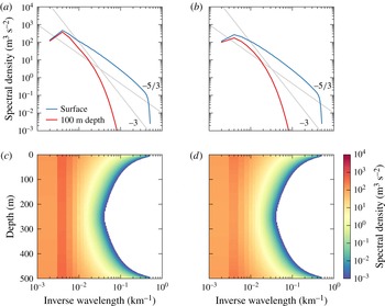
The surface spectra of both kinetic and potential energy peak at a wavelength of approximately 200 km and fall off roughly like
 $\langle K_{k_{h}}\rangle \sim \langle P_{k_{h}}\rangle \sim {k_{h}}^{-5/3}$
(figure 8), as predicted by surface QG turbulence theory for scales smaller than the scales at which mesoscale instabilities inject energy into the system (Blumen Reference Blumen1978). Since small-scale modes decay more rapidly in the vertical than large-scale modes, the spectra are steeper in the interior (e.g. Scott Reference Scott2006). At 100 m depth, the mesoscale energy levels are similar to those at the surface, but submesoscale energy levels are much lower.
Wavenumber spectra of kinetic and potential energy from the thermocline-only simulation. (a) Kinetic and (b) potential energy spectra at the surface and 100 m depth, spectral density of (c) kinetic and (d) potential energy in the wavenumber–depth plane. In (c,d), no values below
 $10^{-3}~\text{m}^{3}~\text{s}^{-2}$
are shown. Reference lines with slopes
 $-3$
and
 $-5/3$
are shown in grey.

A useful diagnostic of turbulent dynamics is the spectral energy budget (e.g. Larichev & Held Reference Larichev and Held1995; Roullet et al. Reference Roullet, McWilliams, Capet and Molemaker2012). While the dynamics is completely determined by the advection of conserved quantities at the surface and bottom, we first consider the energy budget over the entire depth range. We will take into account the reduced nature of these models below, where we present a vertically integrated energy budget for the mixed-layer-only case.
The equations for the spectral perturbation potential and kinetic energies are
 $$\begin{eqnarray}\displaystyle & \displaystyle \frac{\partial P_{k,l}}{\partial t}=\text{Re}\left[\frac{f{\it\Lambda}}{N^{2}}\hat{v}^{\ast }\hat{b}-{\hat{w}}^{\ast }\hat{b}-\frac{1}{N^{2}}\hat{b}^{\ast }\hat{\text{J}}({\it\psi},b)\right]-(r{k_{h}}^{-2}+{\it\nu}{k_{h}}^{2n})P_{k,l} & \displaystyle\end{eqnarray}$$
 $$\begin{eqnarray}\displaystyle & \displaystyle \frac{\partial K_{k,l}}{\partial t}=\text{Re}\left[-f\frac{\partial }{\partial z}({\hat{w}}^{\ast }\hat{{\it\psi}})+{\hat{w}}^{\ast }\hat{b}+\hat{{\it\psi}}^{\ast }\hat{\text{J}}({\it\psi},{\rm\nabla}^{2}{\it\psi})\right]-(r{k_{h}}^{-2}+{\it\nu}{k_{h}}^{2n})K_{k,l}, & \displaystyle\end{eqnarray}$$
 $\text{Re}$
denotes taking the real part. The Fourier transforms in the square bracket are all understood to be evaluated at the wavenumbers
 $k$
and
 $l$
. The first term on the right-hand side of the potential energy equation represents the extraction of potential energy from the mean flow. The second term represents the conversion from potential to kinetic energy. This term appears as a source term in the kinetic energy budget. The third term in the potential energy budget represents spectral transfer by triadic interactions. The sum of this term over all wavenumbers vanishes. An equivalent spectral transfer term appears in the kinetic energy budget (third term). Kinetic energy can also be distributed vertically by pressure fluxes, represented by the first term in the kinetic energy budget. The vertical integral of this term vanishes. The viscosity terms act as sinks for both potential and kinetic energy – hypoviscosity acting at large scales, hyperviscosity at small scales. We present these budgets averaged azimuthally in wavenumber space and over time.
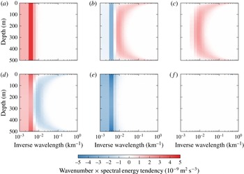
Spectral energy budget for the thermocline-only simulation. The terms are (a) potential energy extraction from the mean, (b) spectral potential energy flux divergence, (c) potential to kinetic energy conversion, (d) kinetic energy flux divergence, including spectral flux and pressure flux, (e) hypoviscosity on both kinetic and potential energy, and (f) hyperviscosity on both kinetic and potential energy. All terms are multiplied by the wavenumber to compensate for logarithmic shrinking.

The extraction of potential energy from the mean is dominated by the largest, most energetic eddies (figure 9
a). The extraction is independent of depth, because
 $q=0$
and therefore
 $$\begin{eqnarray}0=\text{Re}\hat{v}^{\ast }\hat{q}=\text{Re}\frac{\partial }{\partial z}\left(\frac{f}{N^{2}}\hat{v}^{\ast }\hat{b}\right),\end{eqnarray}$$
where it was used that the term involving advection of relative vorticity vanishes. Potential energy is transferred downscale by triadic interactions and deposited near the deformation radius as well as in wedges near the surface and the bottom that reach to much smaller scales (figure 9 b). Where potential energy is deposited by scale interactions, it is converted into kinetic energy (figure 9 c). Near the mesoscale deformation radius, this conversion is due to the mesoscale instability that produces vertical buoyancy fluxes. In the wedges near the surface and bottom, the conversion is due to frontogenesis and secondary instabilities present in the surface QG cascades, which occur independently at the surface and the bottom (Roullet et al. Reference Roullet, McWilliams, Capet and Molemaker2012). The kinetic energy thus created is transferred back to large scales (figure 9 d). The bulk of the energy is dissipated through hypoviscosity at the scales of the largest, most energetic, eddies (figure 9 e). The energy dissipation through hyperviscosity is small, which reflects the fundamental property of geostrophic turbulence that energy is trapped at large scales and viscous energy dissipation vanishes in the limit of infinite resolution and zero (hyper-)viscosity (Kraichnan Reference Kraichnan1967; Charney Reference Charney1971).
4.2. Mixed layer only
We now turn our attention to the nonlinear dynamics of the submesoscale mixed-layer instability and compare its turbulent dynamics to the surface QG turbulence of the thermocline-only case. We study the case with an infinitely deep thermocline, which allows an accurate representation of the submesoscale instability, while eliminating the thermocline instability (figure 5 c,f).
The submesoscale instability grows to finite amplitude and the flow becomes turbulent. There is a turbulent spin-up phase, in which the eddies, which are initially of the size of the instability, grow larger until they reach a statistical equilibrium with hypoviscosity. The flow is host of numerous coherent vortices embedded in a filamentary sea with strong buoyancy gradients (figure 7 c). A snapshot of surface buoyancy appears quite different from the thermocline-only case, but this visual difference is due mostly to the smaller size of the most energetic eddies.
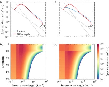
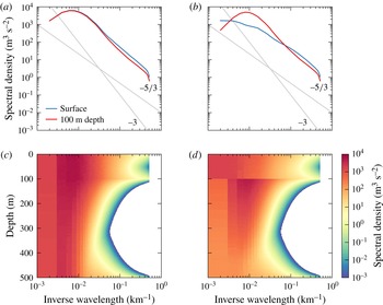
Wavenumber spectra of kinetic and potential energy from the mixed-layer-only simulation. (a) Kinetic and (b) potential energy spectra at the surface and 100 m depth (just below mixed-layer base), spectral density of (c) kinetic and (d) potential energy in the wavenumber–depth plane. In (c,d), no values below
 $10^{-3}~\text{m}^{3}~\text{s}^{-2}$
are shown. Reference lines with slopes
 $-3$
and
 $-5/3$
are shown in grey.

The energy spectra reflect the nearly frontal structure at the surface (figure 10). The kinetic energy spectra fall off slightly more steeply than
 $\langle K_{k_{h}}\rangle \sim {k_{h}}^{-5/3}$
in the scale range of the linear instability and like
 $\langle K_{k_{h}}\rangle \sim {k_{h}}^{-5/3}$
at scales smaller than the linear short-wave cutoff, both at the surface and at the base of the mixed layer at 100 m depth (figure 10
a). The mixed-layer instabilities energize the entire depth of the mixed layer. This is in sharp contrast to the thermocline-only simulation, in which surface QG turbulence energizes a thin wedge close to the surface only.
The equilibrated flow in the mixed-layer-only case is much more energetic than in the thermocline-only case and more energetic than is realistic. While the equilibration by hypoviscosity is unrealistic, we will see that the enhanced energy levels are due to more efficient extraction of mean potential energy in the weakly-stratified mixed layer, which is a dynamical property of the system that does not depend on how the flow is equilibrated. We will discuss possible reasons for these unrealistically high energy levels in § 5.
Below the base of the mixed layer, the potential energy spectra are the same as the kinetic energy spectra (figure 10 c). In the mixed layer, the potential energy spectra are significantly flatter than the kinetic energy spectra. This is in contrast to observations that show rough equipartition between kinetic and potential energy (Callies & Ferrari Reference Callies and Ferrari2013; Callies et al. Reference Callies, Ferrari, Klymak and Gula2015). We currently do not understand the reason for this difference.
The vertical structure of energy shows that the mixed-layer instabilities also energize the thermocline below (figure 10 b,d). At the instability scale, the flow does not reach much into the thermocline. But as the horizontal scale of the flow increases, so does the vertical scale. The flow exhibits the familiar property of geostrophic turbulence and barotropizes as it increases its horizontal scale (Charney Reference Charney1971; Smith & Vallis Reference Smith and Vallis2001).
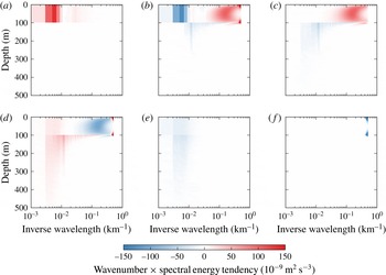
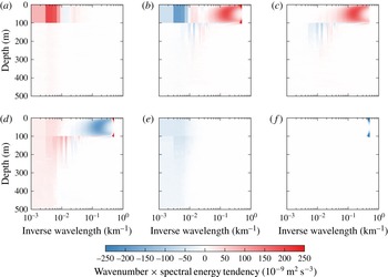
Spectral energy budget for the mixed-layer-only simulation. The terms are (a) potential energy extraction from the mean, (b) spectral potential energy flux divergence, (c) potential to kinetic energy conversion, (d) kinetic energy flux divergence, including spectral flux and pressure flux, (e) hypoviscosity on both kinetic and potential energy and (f) hyperviscosity on both kinetic and potential energy. All terms are multiplied by the wavenumber to compensate for logarithmic shrinking.

The energy transfer into the thermocline is best examined through the spectral energy budget (figure 11). Potential energy is extracted at the scale of the largest, most energetic eddies, but the extraction is confined to the mixed layer (figure 11 a). Potential energy is transferred from the extraction scale to the scale of the mixed-layer instability (figure 11 b). The mixed-layer instability converts potential energy into kinetic energy in the mixed layer, at the instability scale (figure 11 c). The kinetic energy created by the instability undergoes an inverse cascade, in which energy is not only transferred to large horizontal scales, but also vertically into the thermocline (figure 11 d). The deposition of kinetic energy at the scale of the largest eddies is well distributed across the mixed layer and upper thermocline. The vertical distribution of the energy sink through hypoviscosity confirms that the flow extends below the mixed layer at the scale of the largest eddies, where hypoviscosity acts (figure 11 e). Hyperviscosity acts only at the smallest resolved scales (figure 11 f). While small, it does affect the other terms in the budget. We do not discuss its effects any further, because they are expected to disappear if the resolution is increased and the hyperviscosity coefficient decreased.
These energy pathways are reminiscent of the phenomenology of two-layer baroclinic turbulence. The turbulent dynamics of a two-layer system can be understood in terms of a dual cascade (Rhines Reference Rhines and Goldberg1977; Salmon Reference Salmon1978). Baroclinic energy is extracted from the mean at the scale of the largest, most energetic, eddies. The barotropic flow dominates at these scales and transfers the baroclinic energy downscale. The baroclinic mode behaves like a passive tracer at these scales. Around the deformation radius, the instability converts baroclinic energy into barotropic energy. The barotropic energy then enters an inverse cascade, which is arrested at some scale by drag or hypoviscosity. The forward cascade of baroclinic energy is compensated by the inverse cascade of barotropic energy, such that no spectral transfer of total energy occurs. This is consistent with the phenomenology that all sources and sinks of total energy occur at the scale of the largest, most energetic eddies – no energy is dissipated at small scales.
Can the turbulent dynamics induced by mixed-layer instabilities be understood in similar terms? To pursue the analogy, we must first introduce a modal decomposition of the eddy energy. In our system, the vertically integrated total energy can be written entirely in terms of the quantities at the surface and interface:
 $$\begin{eqnarray}E_{k,l}=-{\textstyle \frac{1}{2}}\hat{{\bf\psi}}^{\dagger }\hat{{\bf\theta}}=-{\textstyle \frac{1}{2}}\hat{{\bf\psi}}^{\dagger }\unicode[STIX]{x1D647}\hat{{\bf\psi}},\end{eqnarray}$$
where the conjugate transpose is denoted with a dagger. Since
 $\unicode[STIX]{x1D647}$
is real and symmetric, it can be diagonalized through a unitary matrix
 $\unicode[STIX]{x1D64E}$
,
 $$\begin{eqnarray}\unicode[STIX]{x1D647}=\unicode[STIX]{x1D64E}^{\dagger }\unicode[STIX]{x1D63F}\unicode[STIX]{x1D64E},\end{eqnarray}$$
where
 $\unicode[STIX]{x1D63F}$
is diagonal and consists of the real eigenvalues of
 $\unicode[STIX]{x1D647}$
,
 $\unicode[STIX]{x1D63F}_{jj}={\it\lambda}_{j}$
. The energy can now be written as
 $$\begin{eqnarray}E_{k,l}=-\frac{1}{2}(\unicode[STIX]{x1D64E}\hat{{\bf\psi}})^{\dagger }\unicode[STIX]{x1D63F}(\unicode[STIX]{x1D64E}\hat{{\bf\psi}})=-\frac{1}{2}\mathop{\sum }_{j}{\it\lambda}_{j}|(\unicode[STIX]{x1D64E}\hat{{\bf\psi}})_{j}|^{2}.\end{eqnarray}$$
This defines the modes
 $(\unicode[STIX]{x1D64E}\hat{{\bf\psi}})_{j}$
that are orthogonal with respect to the energy norm, i.e. the energy can be partitioned into contributions
 $E_{k,l}^{j}$
from these modes. The structure of the modes depends on wavenumber, because
 $\unicode[STIX]{x1D647}$
and therefore
 $\unicode[STIX]{x1D64E}$
does.
For the mixed-layer-only case, with
 $\unicode[STIX]{x1D647}$
given by (3.10), the eigenvalues of
 $\unicode[STIX]{x1D647}$
are
 $$\begin{eqnarray}{\it\lambda}_{0,1}=fk_{h}\left(\frac{\coth {\it\mu}_{m}}{N_{m}}+\frac{1}{2N_{t}}\pm \sqrt{\frac{\text{csch}\,^{2}{\it\mu}_{m}}{N_{m}^{2}}+\frac{1}{4N_{t}^{2}}}\right)\end{eqnarray}$$
and we obtain the eigenvectors as the columns of
 $\unicode[STIX]{x1D64E}$
,
 $$\begin{eqnarray}\displaystyle \unicode[STIX]{x1D64E}=\left(\begin{array}{@{}cc@{}}\displaystyle \frac{1}{\left[1+\left(\cosh {\it\mu}_{m}+\displaystyle \frac{N_{m}{\it\lambda}_{0}}{fk_{h}}\sinh {\it\mu}_{m}\right)^{2}\right]^{1/2}} & \displaystyle \frac{1}{\left[1+\left(\cosh {\it\mu}_{m}+\displaystyle \frac{N_{m}{\it\lambda}_{1}}{fk_{h}}\sinh {\it\mu}_{m}\right)^{2}\right]^{1/2}}\\ \displaystyle \frac{\cosh {\it\mu}_{m}+\displaystyle \frac{N_{m}{\it\lambda}_{0}}{fk_{h}}}{\left[1+\left(\cosh {\it\mu}_{m}+\displaystyle \frac{N_{m}{\it\lambda}_{0}}{fk_{h}}\sinh {\it\mu}_{m}\right)^{2}\right]^{1/2}} & \displaystyle \frac{\cosh {\it\mu}_{m}+\displaystyle \frac{N_{m}{\it\lambda}_{1}}{fk_{h}}}{\left[1+\left(\cosh {\it\mu}_{m}+\displaystyle \frac{N_{m}{\it\lambda}_{1}}{fk_{h}}\sinh {\it\mu}_{m}\right)^{2}\right]^{1/2}}\end{array}\right).\hspace{-20.00003pt} & & \displaystyle \nonumber\\ \displaystyle & & \displaystyle\end{eqnarray}$$
For large scales,
 $k_{h}\ll f/N_{t}h$
or
 ${\it\mu}_{m}\ll N_{m}/N_{t}$
, this reduces to
 $$\begin{eqnarray}{\it\lambda}_{0}=-\frac{fk_{h}}{2N_{t}},\quad {\it\lambda}_{1}=-\frac{2f^{2}}{N_{m}^{2}h},\end{eqnarray}$$
and simply
 $$\begin{eqnarray}\unicode[STIX]{x1D64E}=\frac{1}{\sqrt{2}}\left(\begin{array}{@{}cc@{}}1 & 1\\ 1 & -1\end{array}\right).\end{eqnarray}$$
Equation (4.13) indicates that at large scales, the first mode is barotropic in the mixed layer. It behaves like a surface QG mode penetrating into the thermocline. The streamfunction is proportional to
 $k_{h}$
times the conserved quantity (Held et al.
Reference Held, Pierrehumbert, Garner and Swanson1995),
 $$\begin{eqnarray}(\unicode[STIX]{x1D64E}\hat{{\bf\psi}})_{0}=-\frac{fk_{h}}{2N_{t}}(\unicode[STIX]{x1D64E}\hat{{\bf\theta}})_{0}.\end{eqnarray}$$
The second mode at large scales is baroclinic in the mixed layer. The relation between the streamfunction and the conserved quantity is
 $$\begin{eqnarray}(\unicode[STIX]{x1D64E}\hat{{\bf\psi}})_{1}=-\frac{2f^{2}}{N_{m}^{2}h}(\unicode[STIX]{x1D64E}\hat{{\bf\theta}})_{1},\end{eqnarray}$$
which is independent of
 $k_{h}$
, as expected for a baroclinic mode. These are the same modes as those found in the linear stability analysis for large scales (figure 5
f).
This description of the orthogonal modes as barotropic and baroclinic mixed-layer modes only applies at large scales. At smaller scales, the modes have a more complicated vertical structure (figure 12). At scales smaller than the mixed-layer deformation radius, they morph into modes that are decoupled and localized in the vertical at the surface and at the interface. But for the cascade dynamics to be discussed, the mode structure at large scales is what is most important.
Vertical structure of the streamfunction corresponding to orthogonal modes in the mixed-layer-only case for different wavenumbers
 $k_{h}=2{\rm\pi}/{\it\lambda}$
, with the wavelength
 ${\it\lambda}$
given in the panel titles. For (a–c), the modes are normalized to unity at the interface at 100 m depth; for panel (d), the modes are normalized to have a maximum value of unity. Mode 0 is shown in blue, mode 1 in red. In (a–c), the two modes coincide below the interface. (a) 1000 km wavelength; (b) 100 km wavelength; (c) 10 km wavelength; (d) 1 km wavelength.

We can now consider the energy budget of these modes. We start from the vertically integrated spectral energy budget, written in terms of the conserved quantities and corresponding streamfunctions at the surface and interface:
 $$\begin{eqnarray}\frac{\partial E_{k,l}}{\partial t}=-\text{Re}\hat{{\bf\psi}}^{\dagger }\frac{\partial \hat{{\bf\theta}}}{\partial t}.\end{eqnarray}$$
Using the unitary matrix
 $\unicode[STIX]{x1D64E}$
, we can rewrite this as
 $$\begin{eqnarray}\frac{\partial E_{k,l}}{\partial t}=-\text{Re}\,(\unicode[STIX]{x1D64E}\hat{{\bf\psi}})^{\dagger }\frac{\partial }{\partial t}(\unicode[STIX]{x1D64E}\hat{{\bf\theta}})=-\text{Re}\mathop{\sum }_{j}(\unicode[STIX]{x1D64E}\hat{{\bf\psi}})_{j}^{\ast }\frac{\partial }{\partial t}(\unicode[STIX]{x1D64E}\hat{{\bf\theta}})_{j}\end{eqnarray}$$
and thus split the energy budget into its modal components:
 $$\begin{eqnarray}\frac{\partial E_{k,l}^{j}}{\partial t}=-\text{Re}\,(\unicode[STIX]{x1D64E}\hat{{\bf\psi}})_{j}^{\ast }\frac{\partial }{\partial t}(\unicode[STIX]{x1D64E}\hat{{\bf\theta}})_{j}.\end{eqnarray}$$
The terms on the right-hand side of this budget can be obtained by substituting in the spectral form of the evolution equation (4.1). To separate out the advective interactions of the modes with themselves and with each other, we further expand the nonlinear terms in (4.1), using the distributive property of the Jacobian operator, into
 $$\begin{eqnarray}\text{J}({\bf\psi},{\bf\theta})=\text{J}({\bf\psi}^{0},{\bf\theta}^{0})+\text{J}({\bf\psi}^{0},{\bf\theta}^{1})+\text{J}({\bf\psi}^{1},{\bf\theta}^{0})+\text{J}({\bf\psi}^{1},{\bf\theta}^{1}).\end{eqnarray}$$
Here we split the vectors holding the streamfunction and the conserved quantities at the surface and interface into their modal components,
 $$\begin{eqnarray}\hat{{\bf\psi}}^{j}=\unicode[STIX]{x1D64E}^{\dagger }\unicode[STIX]{x1D64B}_{j}\unicode[STIX]{x1D64E}\hat{{\bf\psi}},\quad \hat{{\bf\theta}}^{j}=\unicode[STIX]{x1D64E}^{\dagger }\unicode[STIX]{x1D64B}_{j}\unicode[STIX]{x1D64E}\hat{{\bf\theta}},\quad {\bf\psi}=\mathop{\sum }_{j}{\bf\psi}^{j},\quad {\bf\theta}=\mathop{\sum }_{j}{\bf\theta}^{j},\end{eqnarray}$$
where
 $\unicode[STIX]{x1D64B}_{j}$
are the projections onto the respective modes,
 $$\begin{eqnarray}\unicode[STIX]{x1D64B}_{0}=\left(\begin{array}{@{}cc@{}}1 & 0\\ 0 & 0\end{array}\right),\quad \unicode[STIX]{x1D64B}_{1}=\left(\begin{array}{@{}cc@{}}0 & 0\\ 0 & 1\end{array}\right).\end{eqnarray}$$
The first term in (4.19) represents the advection of the barotropic mode by the barotropic mode, to use the naming convention introduced above. The second term represents the advection of the baroclinic mode by the barotropic mode, and so on.
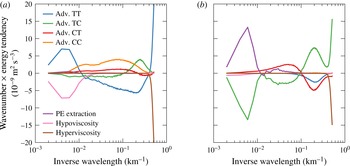
In terms of the orthogonal modes, the energy budget is very similar to that of a baroclinic two-layer system (figure 13, cf. Larichev & Held Reference Larichev and Held1995). The extraction of potential energy from the mean flow is concentrated at the scale of the largest, most energetic, eddies and creates mostly baroclinic energy (figure 13 b). The dominant sink is by hypodiffusion, which also acts on the largest, most energetic, eddies. Barotropic energy dominates at these scales, so hypodiffusion takes out mostly barotropic energy (figure 13 a). The transfer of energy from the baroclinic mode to the barotropic mode occurs through a dual cascade in the submesoscale range. The baroclinic and barotropic energy components are cascaded in opposite directions so as to yield a vanishing spectral transfer of total energy. Baroclinic energy is transferred down to the instability scale, achieved by the advection of the baroclinic mode by the barotropic mode (figure 13 b). The energy deposited around the instability scale is transferred to the barotropic mode by interactions between the two modes, which represents baroclinic instability (figure 13 b). This energy enters the barotropic budget rather less localized in wavenumber space (figure 13 a). An upscale spectral transfer of barotropic energy closes the budget, taking energy from the instability scale to the scale of the largest, most energetic, eddies, where hypodiffusion acts (figure 13 a). Energy loss by hyperdiffusion again enters the budget, but is neglected in this discussion, because it is an artefact of finite resolution.
Modal energy budget for the mixed-layer-only case. The advective terms correspond to the contributions from the four terms in (4.19). The energy tendencies are multiplied by wavenumber to compensate for logarithmic shrinking. (a) Barotropic budget; (b) baroclinic budget.

This model thus exhibits a dual cascade analogous to the classic two-layer system. Baroclinic energy is transferred downscale through advection by the barotropic mode, baroclinic instability converts baroclinic into barotropic energy, and barotropic energy is transferred back upscale in an inverse cascade. The difference is that the barotropic mode at large scales behaves like a surface QG mode, instead of a truly barotropic or two-dimensional mode. The inverse cascade is therefore expected to yield a
 $\langle E_{k_{h}}\rangle \sim k_{h}^{-1}$
surface energy spectrum (Blumen Reference Blumen1978), which we find to emerge if the inertial range is wide enough (not shown). More importantly, the surface-QG-like behaviour implies that in the inverse cascade, energy is transferred to successively larger vertical scales. This provides a pathway for mixed-layer instabilities to energize the thermocline below.
4.3. Full model
We now consider the case with both mesoscale and submesoscale instabilities present. This full model allows us to address how mesoscale thermocline instabilities modify the energy cycle induced by submesoscale mixed-layer instabilities. Furthermore, we pursue a one-to-one comparison between surface-QG dynamics and the dynamics modified by mixed-layer instabilities, with a focus on vertical energy distribution and vertical velocities.
The linear growth rate of the mixed-layer instability is much larger than that of the thermocline instability (figure 5 a), so during the initial transient of the nonlinear simulations the mixed-layer instability grows to finite amplitude first. The evolution in the mixed layer is very similar to that of the mixed-layer-only case: the eddies grow in size until they come into statistical equilibrium with hypoviscosity.
Wavenumber spectra of kinetic and potential energy from the full model simulation. (a) Kinetic and (b) potential energy spectra at the surface and 100 m depth (just below mixed-layer base), spectral density of (c) kinetic and (d) potential energy in the wavenumber–depth plane. In (c,d), no values below
 $10^{-3}~\text{m}^{3}~\text{s}^{-2}$
are shown. Reference lines with slopes
 $-3$
and
 $-5/3$
are shown in grey.

The equilibrated state of the full model is also very similar to that of the mixed-layer-only case in the mixed layer and upper thermocline (figure 14). The energy levels and spectra at the surface and the base of the mixed layer are very similar. Near the bottom, a wedge in wavenumber–depth space is energized in the full model, just like in the thermocline-only case. This is due to surface QG turbulence at the bottom level.
Spectral energy budget for the full model simulation. The terms are (a) potential energy extraction from the mean, (b) spectral potential energy flux divergence, (c) potential to kinetic energy conversion, (d) kinetic energy flux divergence, including spectral flux and pressure flux, (e) hypoviscosity on both kinetic and potential energy, and (f) hyperviscosity on both kinetic and potential energy. All terms are multiplied by the wavenumber to compensate for logarithmic shrinking.

The energy budget is similar to the mixed-layer-only case (figure 15). The main energy pathway is again extraction of potential energy in the mixed layer, transfer to the mixed-layer instability scale, conversion to kinetic energy, transfer back to large scales and into the thermocline and dissipation by hypoviscosity. There is additional energy extraction in the thermocline, but that is weak compared to the extraction in the mixed layer. The dominant dynamics is therefore that described for the mixed-layer-only case. Interaction with the bottom level is possible, but of secondary importance in the parameter regime of relevance.
A different picture emerges when the horizontal buoyancy gradient and the associated geostrophic shear in the mixed layer is (unrealistically) reduced. We choose the mixed-layer shear such that the growth rates of the two instabilities are comparable, which from Eady scaling occurs if
 ${\it\Lambda}_{m}/N_{m}={\it\Lambda}_{t}/N_{t}$
and we set
 ${\it\Lambda}_{m}=2.5\times 10^{-5}~\text{s}^{-1}$
. The horizontal scales of the instabilities and the overall structure of the dispersion curves are the same as those in figure 5(a,d).
This system with reduced mixed-layer shear equilibrates to much lower energy levels than the constant-shear case. The energy levels are comparable to the thermocline-only case and thus allow a one-to-one comparison of the dynamics with and without a mixed layer. The vertical structure of energy in this case with a mixed layer is quite different from the thermocline-only case, because the energy pathway enabled by the mixed-layer instability is still present – mixed-layer instabilities are, on average, not suppressed by the mesoscale strain field (cf. Bishop Reference Bishop1993a ,Reference Bishop b ; Spall Reference Spall1997; McWilliams, Molemaker & Olafsdottir Reference McWilliams, Molemaker and Olafsdottir2009). The mixed-layer instability, while not significantly increasing the mesoscale energy levels, does energize the mixed layer at the submesoscales.
Profiles of root-mean-square vertical velocity for the thermocline-only simulation and the full model simulation with reduced mixed-layer shear.

Concurrent surface buoyancy and vertical velocity snapshots from the full model simulation with reduced mixed-layer shear: (a) surface buoyancy equivalent to figure 7 and (b) vertical velocity at 47 m, the depth of the maximum root mean square vertical velocity.

This difference between mixed-layer dynamics and surface QG turbulence is also reflected in the vertical velocities that are produced by the instabilities (figure 16). While the available potential energies are the same and the resulting surface energy levels comparable between this reduced mixed-layer shear case and the thermocline-only case, there are much larger vertical velocities in the presence of a mixed layer. These enhanced vertical velocities extend significantly below the base of the mixed layer. The largest vertical velocities are located near fronts in the filamentary sea (figure 17). Coherent vortices, while associated with large buoyancy gradients, induce relatively weak vertical motion. The large vertical velocities appear instead to be associated with the filamentary structure generated by mixed-layer instabilities.
The enhancement of vertical velocities in the presence of mixed-layer instabilities can be understood by considering the omega equation (Hoskins et al. Reference Hoskins, Draghici and Davies1978):
 $$\begin{eqnarray}N^{2}{\rm\nabla}^{2}w+f^{2}\frac{\partial ^{2}w}{\partial z^{2}}=-2\boldsymbol{{\rm\nabla}}\boldsymbol{\cdot }\boldsymbol{Q},\end{eqnarray}$$
where
 $$\begin{eqnarray}\boldsymbol{Q}=\left(\frac{\partial \boldsymbol{u}}{\partial x}\boldsymbol{\cdot }\boldsymbol{{\rm\nabla}}b,\frac{\partial \boldsymbol{u}}{\partial y}\boldsymbol{\cdot }\boldsymbol{{\rm\nabla}}b\right).\end{eqnarray}$$
The vertical velocity can be written as a convolution of the Green’s function of (4.22) with the forcing term on the right of (4.22). While the forcing term is not changing much between the cases with and without the mixed layer, the Green’s functions do. The reduced stratification in the mixed layer enhances the response to the forcing term there (Thomas, Tandon & Mahadevan Reference Thomas, Tandon and Mahadevan2008). The enhancement of vertical velocities in our simulation with a mixed layer can thus be attributed to the reduced stratification. Such a reduction of stratification is always associated with a mixed-layer instability, however, so the enhanced vertical velocities are inextricably linked to mixed-layer instabilities.
The forcing term on the right of (4.22) is of the same order in our two cases, because by design the mean states have the same available potential energy and similar submesoscale energy levels are produced. It should be kept in mind, however, that the forcing term does likely increase in the real ocean when mixed layers become deep and mixed-layer instabilities energize the submesoscale range. The more energetic submesoscale turbulence in the wintertime mixed layer is expected to be associated with stronger submesoscale strains than are present in summer (Callies et al. Reference Callies, Ferrari, Klymak and Gula2015). In the wintertime mixed layer, vertical velocities are then enhanced by both a decreased stratification and an increased forcing term on the right of (4.22). Mixed-layer instabilities in the real ocean thus most likely drive an even more dramatic increase in vertical velocities in winter than is present in our simulations with and without mixed layer.
The root-mean-square vertical velocities (figure 16) are similar in structure to those found in primitive equation models (Capet et al. Reference Capet, McWilliams, Molemaker and Shchepetkin2008b ). A careful comparison is necessary to establish whether the QG dynamics described here reproduces the magnitude of the vertical velocities or whether non-QG effects significantly enhance or reduce them (cf. Mahadevan & Tandon Reference Mahadevan and Tandon2006). Such a comparison is beyond the scope of this article.
The interface between mixed layer and thermocline is located at
 $z=-h+{\it\eta}$
, where the interface displacement
 ${\it\eta}$
is determined by requiring the total buoyancy field to be continuous at the interface,
 $$\begin{eqnarray}N_{m}^{2}{\it\eta}+b(-h^{+})=N_{t}^{2}{\it\eta}+b(-h^{-}),\end{eqnarray}$$
where the total buoyancy was linearized around
 $z=-h$
, consistent with QG scaling. The interface is material in the sense that
 $$\begin{eqnarray}\frac{\partial {\it\eta}}{\partial t}+\text{J}({\it\psi},{\it\eta})=w.\end{eqnarray}$$
To leading order, there is therefore no exchange of fluid between mixed layer and thermocline. If non-QG effects are taken into account, however, thermocline waters can be folded into the mixed layer (Garner, Nakamura & Held Reference Garner, Nakamura and Held1992), where atmospherically forced small-scale turbulence can transform them into mixed-layer waters. It thus seems likely that mixed-layer instabilities enhance the exchange between mixed layer and thermocline, but future work will have to investigate what sets the rate of exchange.
5. Comparison to observations
A prominent feature of observed (Callies et al. Reference Callies, Ferrari, Klymak and Gula2015) and modelled (Mensa et al. Reference Mensa, Garraffo, Griffa, Özgökmen, Haza and Veneziani2013; Sasaki et al. Reference Sasaki, Klein, Qiu and Sasai2014) submesoscale flows is their seasonal modulation: they are much more energetic in winter than in summer. This is consistent with an energization of the submesoscale by baroclinic mixed-layer instabilities. Given that these instabilities grow on time scales of order 1 day, they can quickly release large amounts of available potential energy stored in lateral buoyancy gradients in deep winter mixed layers and energize the submesoscale range. Mixed-layer instabilities are instead weak in summer, when mixed layers are shallow and little potential energy is available for release. Mesoscale-driven surface frontogenesis, on the other hand, is not expected to drive a seasonal cycle in submesoscale turbulence, because the mesoscale eddies that generate submesoscale filaments through frontogenesis are about as strong in winter as they are in summer (or even slightly stronger in summer, Qiu (Reference Qiu1999), Qiu & Chen (Reference Qiu and Chen2004) and Sasaki et al. (Reference Sasaki, Klein, Qiu and Sasai2014)).
Submesoscale flows observed in the wintertime Gulf Stream region (Callies et al.
Reference Callies, Ferrari, Klymak and Gula2015) are energetic throughout the deep mixed layer and decay rapidly below. The energy spectra roll off roughly like
 $k_{h}^{-2}$
in the mixed layer and transition to roughly
 $k_{h}^{-3}$
below. This spectral and vertical distribution of energy resembles that produced by our simple model of baroclinic mixed-layer instabilities, which similarly has spectra that roll off roughly like
 $k_{h}^{-2}$
in the mixed layer and more steeply in the thermocline (figure 14). The equilibrated turbulent flow produced by baroclinic mixed-layer instabilities in this model is thus qualitatively consistent with the energetic wintertime submesoscale flows observed in the Gulf Stream region. In summer, on the other hand, submesoscale flows in the Gulf Stream region are weak. The spectral roll off is a rapid
 $k_{h}^{-3}$
, even close to the surface. This lack of submesoscale energy is expected from the lack of energy input from baroclinic mixed-layer instabilities.
There is so far no observational evidence for submesoscale flows that are governed by mesoscale-driven surface frontogenesis as described by surface QG turbulence. The spectral slope of surface kinetic energy may be consistent with the predictions of surface QG theory (e.g. Le Traon et al. Reference Le Traon, Klein, Hua and Dibarboure2008), but the subsurface structure is not. The observations from the Gulf Stream region (Callies et al. Reference Callies, Ferrari, Klymak and Gula2015) show that the spectral and vertical distribution of submesoscale energy is different from that produced by surface QG turbulence (figure 8), in both summer and winter. In winter, submesoscale flows are observed to be energetic throughout the mixed layer – not just in a thin surface layer as predicted by surface QG turbulence. In summer, when baroclinic mixed-layer instabilities are not active and mesoscale-driven surface frontogenesis could dominate, submesoscale flows are observed to be weak – there is no surface-trapped enhancement as predicted by surface QG turbulence. This suggests that these weak summertime submesoscale flows are instead dominated by deep modes generated by mesoscale thermocline instabilities. Observations from Drake Passage also show no signature of mesoscale-driven surface frontogenesis (Rocha et al. Reference Rocha, Chereskin, Gille and Menemenlis2015). Whether it dominates the energization of submesoscale flows elsewhere remains an open question. It may be expected to dominate outside the major current systems, where thermocline instabilities depend on surface buoyancy gradients and can more effectively drive a surface QG cascade (Charney Reference Charney1947; Tulloch et al. Reference Tulloch, Marshall, Hill and Smith2011; Roullet et al. Reference Roullet, McWilliams, Capet and Molemaker2012), but observations are lacking. Balanced submesoscale flows can also be masked by internal waves, especially where mesoscale eddies – and consequently any balanced submesoscale flows – are weak (Richman et al. Reference Richman, Arbic, Shriver, Metzger and Wallcraft2012; Callies & Ferrari Reference Callies and Ferrari2013; Bühler, Callies & Ferrari Reference Bühler, Callies and Ferrari2014; Rocha et al. Reference Rocha, Chereskin, Gille and Menemenlis2015).
Spectra that are observed to fall off like
 $k_{h}^{-3}$
in the seasonal thermocline in summer and in the permanent thermocline throughout the year (Callies et al.
Reference Callies, Ferrari, Klymak and Gula2015) cannot be reproduced by the model formulated in this article. These steep spectra are likely the result of deep Phillips-type instabilities (Phillips Reference Phillips1954) and the potential enstrophy cascade of interior quasi-geostrophic turbulence (Charney Reference Charney1971). Such a cascade is not present in our model, which collapses the interior PV gradients into delta sheets at the interface between mixed layer and thermocline and at the rigid bottom at the base of the thermocline. Our model does capture, however, the steepening of energy spectra below the winter mixed layer – it only lacks the appropriate thermocline dynamics to yield
 $k_{h}^{-3}$
spectra.
The cascade dynamics of our simple QG representation of baroclinic mixed-layer instabilities shows that the mesoscale can effectively be energized by baroclinic mixed-layer instabilities. This would suggest that not only submesoscale but also mesoscale eddies are more energetic in winter than in summer. Altimetry observations (Qiu Reference Qiu1999; Qiu & Chen Reference Qiu and Chen2004) and realistic model simulations (Sasaki et al. Reference Sasaki, Klein, Qiu and Sasai2014), however, suggest that there is not a large modulation of mesoscale energy levels – mesoscale eddies are even slightly stronger in summer than in winter. This lack of wintertime energization of the mesoscale may result from a coupling with unbalanced motions that is not captured by QG dynamics or from an equilibration process that is longer than a season.
The QG model makes the baroclinic mixed-layer instabilities very effective in energizing the entire turbulent flow, because there is no forward energy cascade resulting in small-scale energy dissipation. If non-QG effects were allowed, a fraction of the energy extracted from the mean in the mixed layer would be dissipated at small scales (Capet et al.
Reference Capet, McWilliams, Molemaker and Shchepetkin2008d
). This energy leak to small scales is likely as Rossby and Froude numbers become order 1 at scales of order 1 km. The possibility of an energy leak to small scales was demonstrated by Molemaker et al. (Reference Molemaker, McWilliams and Capet2010), who studied an Eady instability with
 $\mathit{Ro}=\mathit{Fr}=0.5$
, using the full Boussinesq equations. While much of the energy extracted from the mean is still trapped at large scales, as predicted by QG dynamics, some is lost to dissipation at small scales. A small leak of energy in the instability may make a big difference in the cascade dynamics, because that energy is not transferred back to mesoscales, where it would further enhance the extraction of potential energy from the mean. Such an effect could be parameterized in our QG model, but is beyond the scope of this study.
An additional energy sink occurs if the balanced flow interacts with ageostrophic instabilities in the mixed layer. In the presence of geostrophic shear, convective motions forced by the atmosphere are the result of symmetric rather than gravitational instabilities and are slantwise rather than upright (e.g. Emanuel Reference Emanuel1994; Haine & Marshall Reference Haine and Marshall1998; Thomas & Lee Reference Thomas and Lee2005). Symmetric instabilities can extract kinetic energy from the geostrophic shear, so they can drain energy from the balanced flow and increase dissipation (Taylor & Ferrari Reference Taylor and Ferrari2010; Thomas et al. Reference Thomas, Taylor, Ferrari and Joyce2013). This is another way to render the inverse cascade less effective.
Additional sinks for energy in balanced flows in the mixed layer can be the interaction with externally forced near-inertial waves (e.g. Whitt & Thomas Reference Whitt and Thomas2015; Xie & Vanneste Reference Xie and Vanneste2015) and the interaction with surface gravity waves (McWilliams & Fox-Kemper Reference McWilliams and Fox-Kemper2013; Hamlington et al. Reference Hamlington, Van Roekel, Fox-Kemper, Julien and Chini2014). Both may drain enough energy out of the balanced flow to prevent an effective inverse cascade of submesoscale kinetic energy to mesoscales.
QG dynamics further do not allow for a feedback of eddies on the mean stratification of the mixed layer (e.g. Fox-Kemper et al. Reference Fox-Kemper, Ferrari and Hallberg2008), so that no restratification can occur. In the real ocean, the restratification through baroclinic mixed-layer instabilities is opposed by convective and mechanical mixing that is driven by atmospheric forcing. The fixed mean stratification in the QG model assumes that this forced vertical mixing is in balance with restratification. It is unclear whether and how vertical mixing alters the energy budget of the balanced flow in the mixed layer. It is also unclear what the effect of an unsteady atmospheric forcing is, which upsets the balance between vertical mixing and restratification.
Another possible explanation for the lack of a wintertime energization of the mesoscale by baroclinic mixed-layer instabilities is that it takes a few months for the kinetic energy injected by submesoscale mixed-layer instabilities to arrive at the mesoscale (Sasaki et al. Reference Sasaki, Klein, Qiu and Sasai2014). This could also explain the (weak) summer maximum in mesoscale energy (Qiu Reference Qiu1999; Qiu & Chen Reference Qiu and Chen2004). This time dependence is not addressed in our simple model of baroclinic mixed-layer instabilities, in which we prescribe perpetual winter conditions. If the time scale of turbulent equilibration is not much shorter than the seasonal time scale, it is likely that submesoscale – and possibly mesoscale – flows are not in statistical equilibrium. It remains to be investigated how a seasonally modulated mixed layer modifies the inverse cascade and the energization of the mesoscale by baroclinic mixed-layer instabilities.
Realistic high-resolution simulations of the type employed by Shcherbina et al. (Reference Shcherbina, D’Asaro, Lee, Klymak, Molemaker and McWilliams2013), Sasaki et al. (Reference Sasaki, Klein, Qiu and Sasai2014), Gula, Molemaker & McWilliams (Reference Gula, Molemaker and McWilliams2015) may be able to address these caveats and bridge the gap between observations and the idealized QG dynamics described here. These primitive equation and Boussinesq simulations can provide insights into how non-QG effects modify the submesoscale dynamics induced by mixed-layer instabilities. An exploration of non-QG effects in more idealized set-ups may also prove useful. Primitive equation and Boussinesq simulations can also address how non-QG effects modify mesoscale-driven surface frontogenesis and allow an estimate of the importance of corrections to surface QG turbulence (cf. Hakim et al. Reference Hakim, Snyder and Muraki2002; Capet et al. Reference Capet, McWilliams, Molemaker and Shchepetkin2008c ; Klein et al. Reference Klein, Hua, Lapeyre, Capet, Le Gentil and Sasaki2008; Badin Reference Badin2012; Roullet et al. Reference Roullet, McWilliams, Capet and Molemaker2012), providing another stepping stone for understanding observations.
6. Conclusions
The simple model formulated in this article sharpens our understanding of how baroclinic mixed-layer instabilities can energize submesoscale turbulence and how this mechanism differs from mesoscale-driven surface frontogenesis. Our analysis suggests that the presence of a mixed layer has a profound effect on submesoscale turbulence. Lateral buoyancy gradients, combined with the low stratification in the mixed layer, provide a large amount of available potential energy that can be extracted by baroclinic instabilities in the mixed layer. The extraction of available potential energy from the large-scale mean is dominated by mesoscale eddies, but potential energy is subsequently transferred downscale to the deformation radius of the mixed layer, where baroclinic instability converts it into kinetic energy. In the QG dynamics considered here, the energy lost to small scales is negligible. The entire energy extracted from the mean in the mixed layer is converted to kinetic energy around the deformation radius of the mixed layer and subsequently transferred back to larger scales in an inverse cascade that also energizes the thermocline below. Through this process, baroclinic mixed-layer instabilities can energize the submesoscale range and even the mesoscale eddy field.
This turbulent dynamics follows a dual cascade similar to that present in two-layer QG flow (Rhines Reference Rhines and Goldberg1977; Salmon Reference Salmon1978; Larichev & Held Reference Larichev and Held1995) and in idealized continuously stratified QG flows (Smith & Vallis Reference Smith and Vallis2002) – but with mixed-layer modes. The energy in the baroclinic mode, which is baroclinic in the mixed layer and does not reach much into the thermocline, is transferred downscale through advection by the barotropic mode, which is barotropic in the mixed layer and decays surface-QG-like in the thermocline. Around the deformation radius of the mixed layer, baroclinic instability transforms baroclinic into barotropic energy, which then enters an inverse cascade.
The dynamics resulting from baroclinic mixed-layer instabilities substantially differs from mesoscale-driven surface frontogenesis, as described by surface QG turbulence forced by a mesoscale eddy field, which is often invoked to explain energetic submesoscales. Surface QG turbulence can only energize a thin surface layer. Mixed-layer instabilities, instead, energize the entire depth of the mixed layer. Vertical velocities are drastically enhanced in the presence of baroclinic mixed-layer instabilities compared to surface QG flows of similar energy levels.
The enhancement of submesoscale energy throughout the mixed layer and the decay below its base, as generated by baroclinic mixed-layer instabilities, are consistent with wintertime observations from the Gulf Stream region (Callies et al. Reference Callies, Ferrari, Klymak and Gula2015). These observations, as well as models (Mensa et al. Reference Mensa, Garraffo, Griffa, Özgökmen, Haza and Veneziani2013; Sasaki et al. Reference Sasaki, Klein, Qiu and Sasai2014), also show that submesoscale flows are most energetic in winter, when baroclinic mixed-layer instabilities are active. This evidence points to the importance of baroclinic mixed-layer instabilities in energizing the submesoscale.
It remains to be investigated how deviations from QG dynamics affect submesoscale flows when a mixed layer is present. The restratification by mixed-layer instabilities, the formation of buoyancy discontinuities, ageostrophic instabilities and forced mixed-layer turbulence all have the potential to modify the leading-order balanced dynamics described here. For example, it remains unclear how much of the submesoscale kinetic energy generated by baroclinic mixed-layer instabilities is cascaded to mesoscales, how vertical velocities are modified by non-QG effects and how the enhancement of vertical velocities by mixed-layer instabilities translates into an exchange of fluid between mixed layer and thermocline.
It is hoped that the model and dynamics discussed here in an oceanographic context are of interest in a broader geophysical fluid dynamics context. Atmospheres often display layers of different stratification, which likely induce similar dynamics. These have partly been explored for the terrestrial atmosphere and it seems likely that similar dynamics also occur in the atmospheres of other planets.
Acknowledgements
Much of this work was conducted at the Geophysical Fluid Dynamics Summer School at the Woods Hole Oceanographic Institution. We gratefully acknowledge the NSF’s support of this program and the fruitful interactions we had with staff and visitors.
Appendix A
A QG system of
 $n$
layers of constant PV, of thickness
 $h_{j}$
and stratification
 $N_{j}$
, consists of
 $n+1$
conserved quantities that are advected by the geostrophic flow at their respective levels. Compared to the two-layer model considered in the main text, additional interface quantities analogous to
 ${\it\theta}_{1}$
are present. The linear operator in the inversion relation (2.9a
) has tridiagonal structure:
 $$\begin{eqnarray}\displaystyle \hspace{-5.0pt}\unicode[STIX]{x1D647}=fk_{h}\left(\begin{array}{@{}ccccc@{}}\displaystyle -\frac{\coth {\it\mu}_{0}}{N_{0}} & \displaystyle \frac{\text{csch}\,{\it\mu}_{0}}{N_{0}}\\ \displaystyle \frac{\text{csch}\,{\it\mu}_{0}}{N_{0}} & \displaystyle -\frac{\coth {\it\mu}_{0}}{N_{0}}-\frac{\coth {\it\mu}_{1}}{N_{1}} & \displaystyle \frac{\text{csch}\,{\it\mu}_{1}}{N_{1}}\\ & \ddots & \ddots & \ddots \\ & & \displaystyle \frac{\text{csch}\,{\it\mu}_{n-1}}{N_{n-1}} & \displaystyle -\frac{\coth {\it\mu}_{n-1}}{N_{n-1}}-\frac{\coth {\it\mu}_{n}}{N_{n}} & \displaystyle \frac{\text{csch}\,{\it\mu}_{n}}{N_{n}}\\ & & & \displaystyle \frac{\text{csch}\,{\it\mu}_{n}}{N_{n}} & \displaystyle -\frac{\coth {\it\mu}_{n}}{N_{n}}\end{array}\right),\hspace{-20.00003pt} & & \displaystyle \nonumber\\ \displaystyle & & \displaystyle\end{eqnarray}$$
where
 ${\it\mu}_{j}=N_{j}k_{h}h_{j}/f$
. It may be more efficient to solve the inversion relation numerically instead of calculating the inverse of this matrix, which will generally be full.
One can also include a PV gradient due to differential rotation. This can be done using a trick described by Lindzen (Reference Lindzen1994): instead of using linear shear and constant stratification in the layers, one can use parabolic shear or a modified stratification profile, which allows cancellation of the contribution from the
 ${\it\beta}$
-effect and retaining constant PV within the layers. The PV gradient due to
 ${\it\beta}$
is then included in the PV sheets at the interfaces.
Appendix B
If there is a buoyancy jump
 $g^{\prime }$
at the interface, the matching conditions must be modified. To ensure a continuous pressure at the interface at
 $z=-h+{\it\eta}$
, we require
 $$\begin{eqnarray}{\it\psi}(-h^{+})-{\it\psi}(-h^{-})=-\frac{g^{\prime }}{f}{\it\eta}.\end{eqnarray}$$
Here,
 ${\it\eta}$
is the perturbation of the interface between the constant-PV layers. The buoyancy equations (2.2) and (2.3) can be combined with the kinematic condition
 $$\begin{eqnarray}w=\frac{\partial {\it\eta}}{\partial t}+\text{J}({\it\psi},{\it\eta}),\end{eqnarray}$$
applied at
 $z=-h^{+}$
and
 $z=-h^{-}$
, to give
 $$\begin{eqnarray}\frac{\partial {\it\theta}_{1}}{\partial t}+\text{J}({\it\psi}_{1},{\it\theta}_{1})=0,\quad \frac{\partial {\it\theta}_{2}}{\partial t}+\text{J}({\it\psi}_{2},{\it\theta}_{2})=0,\end{eqnarray}$$
where
 $$\begin{eqnarray}{\it\theta}_{1}=f\frac{b(-h^{+})}{N_{m}^{2}}+f{\it\eta},\quad {\it\theta}_{2}=f\frac{b(-h^{-})}{N_{t}^{2}}+f{\it\eta},\quad {\it\psi}_{1}={\it\psi}(-h^{+}),\quad {\it\psi}_{2}={\it\psi}(-h^{-}).\end{eqnarray}$$
Together with the conservation of surface and bottom buoyancy,
 $$\begin{eqnarray}{\it\theta}_{0}=-f\frac{b(0)}{N_{m}^{2}},\quad {\it\theta}_{3}=f\frac{b(-H)}{N_{t}^{2}},\end{eqnarray}$$
and the inversion relation obtained by solving (2.10) with the matching conditions above, the model is complete. It now consists of four conserved quantities.