
1 Introduction
Cohesive sediment, commonly defined as particles with diameters  $D_{p}<63~\unicode[STIX]{x03BC}\text{m}$, plays a central role in a wide range of environmental and industrial processes. For these small grain sizes, attractive van der Waals forces can outweigh hydrodynamic, buoyancy and collision forces, and trigger the formation of large aggregates via flocculation (Yoshimasa Reference Yoshimasa2017). Following the pioneering work by Levich (Reference Levich1962), current approaches for modelling the flocculation process often employ population balance equations (Maggi, Mietta & Winterwerp Reference Maggi, Mietta and Winterwerp2007; Verney et al. Reference Verney, Lafite, Burn-Cottan and le Hir2011; Shin, Son & Lee Reference Shin, Son and Lee2015) or simplified versions thereof (Winterwerp Reference Winterwerp1998; Son & Hsu Reference Son and Hsu2008, Reference Son and Hsu2009; Lee et al. Reference Lee, Toorman, Molz and Wang2011; Shen et al. Reference Shen, Lee, Fettweis and Toorman2018). These semi-empirical models, which require calibration with experimental data, usually do not account for the detailed profiles of the various forces governing particle–particle interactions.
The present investigation presents a conceptually simple model to obtain flocculation data via one-way coupled simulations that track individual primary particles and accurately capture the inter-particle forces, based on the recent development of advanced collision models in viscous flows (Biegert, Vowinckel & Meiburg (Reference Biegert, Vowinckel and Meiburg2017a), and references therein), along with strategies for accurately modelling cohesive forces (Vowinckel et al. Reference Vowinckel, Withers, Luzzatto-Fegiz and Meiburg2019). Towards this end, we employ the well-known initial configuration of cellular Taylor–Green flow as a simple, quasi-steady analytical model of a turbulent flow at the Kolmogorov scale. This flow has previously been used successfully in elucidating fundamental aspects of particle–vortex interactions (Maxey Reference Maxey1987; Bergougnoux et al. Reference Bergougnoux, Bouchet, Lopez and Guazzelli2014). We will exploit this conceptually simple, computationally efficient scenario to systematically investigate the influence of key physical parameters, and propose a new flocculation model that agrees closely with experimental data.
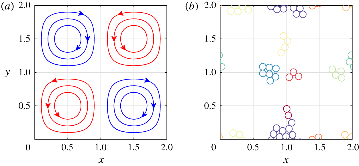
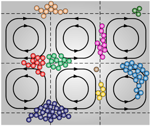
(a) Streamlines of the doubly periodic background flow. (b) Typical floc configuration made up of spherical primary particles, with individual flocs distinguished by colour.

2 Computational model
2.1 Particle motion in cellular flow fields
In the spirit of earlier investigations by Maxey (Reference Maxey1987) and Bergougnoux et al. (Reference Bergougnoux, Bouchet, Lopez and Guazzelli2014), we apply a simple model flow in order to investigate the effects of turbulence on the dynamics of cohesive particles. We consider the one-way coupled motion of small spherical particles in the two-dimensional, steady, spatially periodic cellular flow field commonly employed as initial condition for simulating Taylor–Green vortices (cf. figure 1a), with fluid velocity field  $\boldsymbol{u}_{f}=(u_{f},v_{f})^{\text{T}}$
 $$\begin{eqnarray}u_{f}={\displaystyle \frac{U_{0}}{\unicode[STIX]{x03C0}}}\sin \left({\displaystyle \frac{\unicode[STIX]{x03C0}x}{L}}\right)\cos \left({\displaystyle \frac{\unicode[STIX]{x03C0}y}{L}}\right),\quad v_{f}=-{\displaystyle \frac{U_{0}}{\unicode[STIX]{x03C0}}}\cos \left({\displaystyle \frac{\unicode[STIX]{x03C0}x}{L}}\right)\sin \left({\displaystyle \frac{\unicode[STIX]{x03C0}y}{L}}\right),\end{eqnarray}$$
where  $L$ and
 $U_{0}$ represent the characteristic length and velocity scales of the vortex flow.
Keeping in mind that cohesive sediment grains in nature may be non-spherical, we nevertheless approximate each primary particle  $i$ as a sphere that moves with the translational velocity
 $\boldsymbol{u}_{p,i}=(u_{p,i},v_{p,i})^{\text{T}}$ and the angular velocity
 $\unicode[STIX]{x1D714}_{p,i}$. These are obtained from the linear and angular momentum equations
 $$\begin{eqnarray}\displaystyle & \displaystyle m_{p}{\displaystyle \frac{\text{d}\boldsymbol{u}_{p,i}}{\text{d}t}}=\boldsymbol{F}_{d,i}+\boldsymbol{F}_{g,i}+\underbrace{\mathop{\sum }_{j=1,j\neq i}^{N_{p}}(\boldsymbol{F}_{con,ij}+\boldsymbol{F}_{lub,ij}+\boldsymbol{F}_{coh,ij})}_{\boldsymbol{F}_{c,i}}, & \displaystyle\end{eqnarray}$$
 $$\begin{eqnarray}\displaystyle & \displaystyle I_{p}{\displaystyle \frac{\text{d}\unicode[STIX]{x1D74E}_{p,i}}{\text{d}t}}=\underbrace{\mathop{\sum }_{j=1,j\neq i}^{N_{p}}(\boldsymbol{T}_{con,ij}+\boldsymbol{T}_{lub,ij})}_{\boldsymbol{T}_{c,i}}, & \displaystyle\end{eqnarray}$$
where the primary particle  $i$ moves in response to the Stokes drag force
 $\boldsymbol{F}_{d,i}=-3\unicode[STIX]{x03C0}D_{p}\unicode[STIX]{x1D707}_{f}(\boldsymbol{u}_{p,i}-\boldsymbol{u}_{f,i})$, the gravitational force
 $\boldsymbol{F}_{g,i}=\unicode[STIX]{x03C0}D_{p}^{3}(\unicode[STIX]{x1D70C}_{p}-\unicode[STIX]{x1D70C}_{f})\boldsymbol{g}/6$, and the particle–particle interaction force
 $\boldsymbol{F}_{c,i}$. Here
 $\boldsymbol{u}_{f,i}$ and
 $\boldsymbol{u}_{p,i}$ indicate the fluid and particle velocities evaluated at the particle centre, and
 $m_{p}$ denotes the particle’s mass,
 $D_{p}$ its diameter,
 $\unicode[STIX]{x1D70C}_{p}$ its density, and
 $N_{p}$ the total number of particles in the flow. We assume all particles to have the same diameter and density. Here
 $\unicode[STIX]{x1D707}_{f}$ and
 $\unicode[STIX]{x1D70C}_{f}$ denote the dynamic viscosity and the density of the fluid, respectively, and
 $\boldsymbol{g}$ is the gravitational acceleration;
 $\boldsymbol{F}_{c,i}$ accounts for the direct contact force
 $\boldsymbol{F}_{con,ij}$ in the normal and tangential directions, as well as for short-range forces due to lubrication
 $\boldsymbol{F}_{lub,ij}$ and cohesion
 $\boldsymbol{F}_{coh,ij}$, where the subscript
 $ij$ indicates the interaction between particles
 $i$ and
 $j$;
 $I_{p}=\unicode[STIX]{x03C0}\unicode[STIX]{x1D70C}_{p}D_{p}^{5}/60$ denotes the moment of inertia of a particle; and
 $\boldsymbol{T}_{c,i}$ represents the torque due to particle–particle interactions, where we distinguish between the direct contact torque
 $\boldsymbol{T}_{con,ij}$ and lubrication torque
 $\boldsymbol{T}_{lub,ij}$.
Following Biegert et al. (Reference Biegert, Vowinckel and Meiburg2017a), we represent the direct contact force  $\boldsymbol{F}_{con,ij}$ by means of spring–dashpot functions, while the lubrication force
 $\boldsymbol{F}_{lub,ij}$ is accounted for based on Cox & Brenner (Reference Cox and Brenner1967), as implemented in Biegert et al. (Reference Biegert, Vowinckel, Ouillon and Meiburg2017b). The model for the cohesive force
 $\boldsymbol{F}_{coh,ij}$ is based on the work of Vowinckel et al. (Reference Vowinckel, Withers, Luzzatto-Fegiz and Meiburg2019). It assumes a parabolic force profile, distributed over a thin shell surrounding each particle.
2.2 Non-dimensionalization
We choose  $L$,
 $U_{0}$ and
 $L/U_{0}$ as the characteristic length, velocity and time scales. Conceptually, these can be thought of as representing Kolmogorov scales. In this way, we obtain the dimensionless equation of motion for the particles as
 $$\begin{eqnarray}\tilde{m}_{p}{\displaystyle \frac{\text{d}\tilde{\boldsymbol{u}}_{p,i}}{\text{d}\tilde{t}}}=\underbrace{-{\displaystyle \frac{\tilde{m}_{p}(\tilde{\boldsymbol{u}}_{p,i}-\tilde{\boldsymbol{u}}_{f,i})}{St}}}_{\tilde{\boldsymbol{F}}_{d,i}}+\underbrace{{\displaystyle \frac{\tilde{m}_{p}\tilde{W}}{St}}}_{\tilde{\boldsymbol{F}}_{g,i}}+\mathop{\sum }_{j=1,j\neq i}^{N_{p}}(\tilde{\boldsymbol{F}}_{con,ij}+\tilde{\boldsymbol{F}}_{lub,ij}+\tilde{\boldsymbol{F}}_{coh,ij}),\end{eqnarray}$$
where dimensionless quantities are denoted by a tilde. The dynamics of the primary particles are characterized by the Stokes number  $St=U_{0}\unicode[STIX]{x1D70C}_{p}D_{p}^{2}/(18L\unicode[STIX]{x1D707}_{f})$ and the settling velocity
 $\tilde{W}=v_{s}/U_{0}$, where
 $v_{s}=(\unicode[STIX]{x1D70C}_{p}-\unicode[STIX]{x1D70C}_{f})D_{p}^{2}\boldsymbol{g}/(18\unicode[STIX]{x1D707}_{f})$ is the Stokes settling velocity of an individual, isolated primary particle. The dimensionless particle mass and density ratio are defined as
 $\tilde{m}_{p}=\unicode[STIX]{x03C0}\tilde{D}_{p}^{3}\tilde{\unicode[STIX]{x1D70C}}_{s}/6$ and
 $\tilde{\unicode[STIX]{x1D70C}}_{s}=\unicode[STIX]{x1D70C}_{p}/\unicode[STIX]{x1D70C}_{f}$, respectively.
The dimensionless direct contact force  $\tilde{\boldsymbol{F}}_{con,ij}$ between particles includes the normal component
 $\tilde{\boldsymbol{F}}_{con,n,ij}$ and the tangential component
 $\tilde{\boldsymbol{F}}_{con,t,ij}$, which are defined as
 $$\begin{eqnarray}\tilde{\boldsymbol{F}}_{con,ij}=\left\{\begin{array}{@{}ll@{}}\underbrace{-\tilde{k}_{n}|\tilde{\unicode[STIX]{x1D701}}_{n,ij}-\tilde{\unicode[STIX]{x1D701}}_{min}|^{3/2}\boldsymbol{n}-\tilde{d}_{n}\tilde{\boldsymbol{v}}_{n,ij}}_{\tilde{\boldsymbol{F}}_{con,n,ij}}+\\ \underbrace{\min (-\tilde{k}_{t}\tilde{\unicode[STIX]{x1D701}}_{t,ij}-\tilde{d}_{t}\tilde{\boldsymbol{v}}_{t,ij},\Vert \,f\tilde{\boldsymbol{F}}_{con,n,ij}\Vert )\boldsymbol{t}}_{\tilde{\boldsymbol{F}}_{con,t,ij}}, & \tilde{\unicode[STIX]{x1D701}}_{n,ij}\leqslant \tilde{\unicode[STIX]{x1D701}}_{min},\\ 0, & \text{otherwise},\end{array}\right.\end{eqnarray}$$
where  $\tilde{\unicode[STIX]{x1D701}}_{n,ij}$ is the normal surface distance between particles
 $i$ and
 $j$. We account for the surface roughness of the particles, which is set to
 $\tilde{\unicode[STIX]{x1D701}}_{min}=0.0015\tilde{D}_{p}$. Here
 $\tilde{\unicode[STIX]{x1D701}}_{t,ij}$ is the tangential spring displacement, which denotes the accumulated relative tangential motion between two particles in contact;
 $\tilde{\boldsymbol{v}}_{n,ij}$ and
 $\tilde{\boldsymbol{v}}_{t,ij}$ denote the normal and tangential components of the relative velocity of particles
 $i$ and
 $j$;
 $\boldsymbol{n}$ represents the outward-pointing normal on the particle surface; and
 $\boldsymbol{t}$ points in the direction of the tangential force. We use the parametrization for silicate grains described in Biegert et al. (Reference Biegert, Vowinckel and Meiburg2017a), so that we chose a standard friction coefficient of
 $f=0.15$ and obtain stiffness
 $\tilde{k}_{n}$ and
 $\tilde{k}_{t}$ and damping
 $\tilde{d}_{n}$ and
 $\tilde{d}_{t}$ to obtain a specified restitution coefficient as the ratio of impact to rebound velocity (
 $e_{n}=0.97$) for the normal component and rolling conditions for the tangential component of
 $\tilde{\boldsymbol{F}}_{con,ij}$, respectively.
The dimensionless lubrication force  $\tilde{\boldsymbol{F}}_{lub,ij}$ between particles
 $i$ and
 $j$ has the normal and tangential components
 $\tilde{\boldsymbol{F}}_{lub,n,ij}$ and
 $\tilde{\boldsymbol{F}}_{lub,t,ij}$, respectively, which are defined as
 $$\begin{eqnarray}\tilde{\boldsymbol{F}}_{lub,ij}=\left\{\begin{array}{@{}ll@{}}\underbrace{-{\displaystyle \frac{\tilde{m}_{p}\tilde{D}_{p}\tilde{\boldsymbol{v}}_{n,ij}}{8St\tilde{\unicode[STIX]{x1D701}}_{n,ij}}}}_{\tilde{\boldsymbol{F}}_{lub,n,ij}}+\underbrace{{\displaystyle \frac{\tilde{m}_{p}}{2St}}(k_{1}\tilde{\boldsymbol{u}}_{t,ij}+k_{2}\tilde{\boldsymbol{w}}_{t,ij})}_{\tilde{\boldsymbol{F}}_{lub,t,ij}}, & \tilde{\unicode[STIX]{x1D701}}_{min}<\tilde{\unicode[STIX]{x1D701}}_{n,ij}\leqslant \tilde{h},\\ 0, & \text{otherwise},\end{array}\right.\end{eqnarray}$$
where  $\tilde{h}=\tilde{D}_{p}/10$ is the range of the lubrication force. Here
 $\tilde{\boldsymbol{u}}_{t,ij}$ and
 $\tilde{\boldsymbol{w}}_{t,ij}$ denote the tangential components of the relative translational velocity and the relative rotational velocity of the particles, respectively. The coefficients
 $k_{1}$ and
 $k_{2}$ take the values
 $k_{1}=0.53\ln (4\tilde{\unicode[STIX]{x1D701}}_{n,ij}/\tilde{D}_{p})-0.9588$ and
 $k_{2}=0.13\ln (4\tilde{\unicode[STIX]{x1D701}}_{n,ij}/\tilde{D}_{p})-0.2526$, respectively (Biegert et al. Reference Biegert, Vowinckel, Ouillon and Meiburg2017b).
The dimensionless cohesive force  $\tilde{\boldsymbol{F}}_{coh,ij}$ is defined as
 $$\begin{eqnarray}\tilde{\boldsymbol{F}}_{coh,ij}=\left\{\begin{array}{@{}ll@{}}-4Co{\displaystyle \frac{\tilde{\unicode[STIX]{x1D701}}_{n,ij}^{2}-\tilde{\unicode[STIX]{x1D706}}\tilde{\unicode[STIX]{x1D701}}_{n,ij}}{\tilde{\unicode[STIX]{x1D706}}^{2}}}\boldsymbol{n}, & \tilde{\unicode[STIX]{x1D701}}_{min}<\tilde{\unicode[STIX]{x1D701}}_{n,ij}\leqslant \tilde{\unicode[STIX]{x1D706}},\\ 0, & \text{otherwise},\end{array}\right.\end{eqnarray}$$
where  $\tilde{\unicode[STIX]{x1D706}}=\tilde{h}/2=\tilde{D}_{p}/20$ represents the range of the cohesive force. The cohesive number
 $Co$ indicates the ratio of the maximum cohesive force
 $\Vert \boldsymbol{F}_{coh,ij}\Vert$ at
 $\tilde{\unicode[STIX]{x1D701}}_{n,ij}=\tilde{\unicode[STIX]{x1D706}}/2$ to the characteristic inertial force
 $$\begin{eqnarray}Co={\displaystyle \frac{\max (\Vert \boldsymbol{F}_{coh,ij}\Vert )}{U_{0}^{2}L^{2}\unicode[STIX]{x1D70C}_{f}}}={\displaystyle \frac{A_{H}D_{p}}{16\unicode[STIX]{x1D706}\unicode[STIX]{x1D701}_{0}}}{\displaystyle \frac{1}{U_{0}^{2}L^{2}\unicode[STIX]{x1D70C}_{f}}},\end{eqnarray}$$
where the Hamaker constant  $A_{H}$ is a function of the particle and fluid properties and the characteristic distance
 $\unicode[STIX]{x1D701}_{0}=0.00025D_{p}$. Vowinckel et al. (Reference Vowinckel, Withers, Luzzatto-Fegiz and Meiburg2019) provide representative values of
 $A_{H}$ for common natural systems.
To summarize, the simulations require as input parameters the dimensionless particle diameter  $\tilde{D}_{p}$, the number of particles
 $N_{p}$, the density ratio
 $\tilde{\unicode[STIX]{x1D70C}}_{s}$, the settling velocity
 $\tilde{W}$, the Stokes number
 $St$ and the cohesive number
 $Co$. For convenience, the tilde symbol will be omitted henceforth.
2.3 Validation: aggregation and breakage of two particles
To validate our numerical implementation of the cohesive force model, we consider the interaction of two neutrally buoyant particles with  $D_{p}=0.1$,
 $St=0.1$,
 $W=0$ that are placed symmetrically to the left and right of the stagnation point at (1,1) in figure 1(a). The particles are at rest initially, at a surface distance of
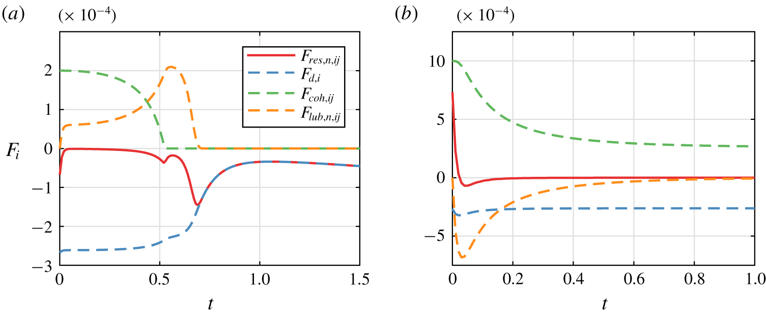
 $\unicode[STIX]{x1D706}/2=0.0025$, so that the cohesive force is at its maximum. Figure 2 presents the temporal evolution of the various forces acting on the particle to the left of the stagnation point, for the two scenarios of (a) floc breakage and (b) floc aggregation. For the smaller value of
 $Co$, the drag force that tries to separate the particles is initially larger than the cohesive force that attracts them to each other (figure 2a). As the surface distance between the particles increases, the cohesive force decays and approaches zero. While the lubrication force
 $F_{lub,n,ij}$ acts to slow the separation of the particles, the overall net force
 $F_{res,n,ij}$ acting on the particle is always negative, so that the particles gradually move apart. When the surface distance between the particles becomes larger than the range of the cohesive and lubrication forces, the net force equals the drag force.
Figure 2(b), on the other hand, focuses on a case in which the cohesive force initially is larger than the drag force, so that the particles approach each other. This process is slowed down by the lubrication force. The particles asymptotically approach an equilibrium position of near contact in which the separating drag force is balanced by the attractive cohesive force.
Transient forces on the particle to the left of the stagnation point at (1,1) in figure 1(a), during binary interaction. The simulation parameters are  $D_{p}=0.1$,
 $\unicode[STIX]{x1D70C}_{s}=1$,
 $St=0.1$,
 $W=0$: (a) breakage,
 $Co=2\times 10^{-4}$; (b) aggregation,
 $Co=1\times 10^{-3}$.

3 Large ensemble of particles
3.1 Computational set-up
We now investigate ensembles involving more particles, to obtain insight into the flocculation dynamics of larger systems. We employ a computational domain of size  $L_{x}\times L_{y}=2\times 2$, with periodic boundaries (figure 1a). All particles have identical diameters and densities. Initially they are at rest and separated, and randomly distributed throughout the domain. When the distance between two particles is less than
 $\unicode[STIX]{x1D706}/2$, we consider them as part of the same floc. We then track the number of flocs
 $N_{f}$ as a function of time, with an individual particle representing the smallest possible floc. To improve the statistics, we repeat each simulation five times for different random initial conditions, as the simulation results are statistically independent of the initial particle placement.
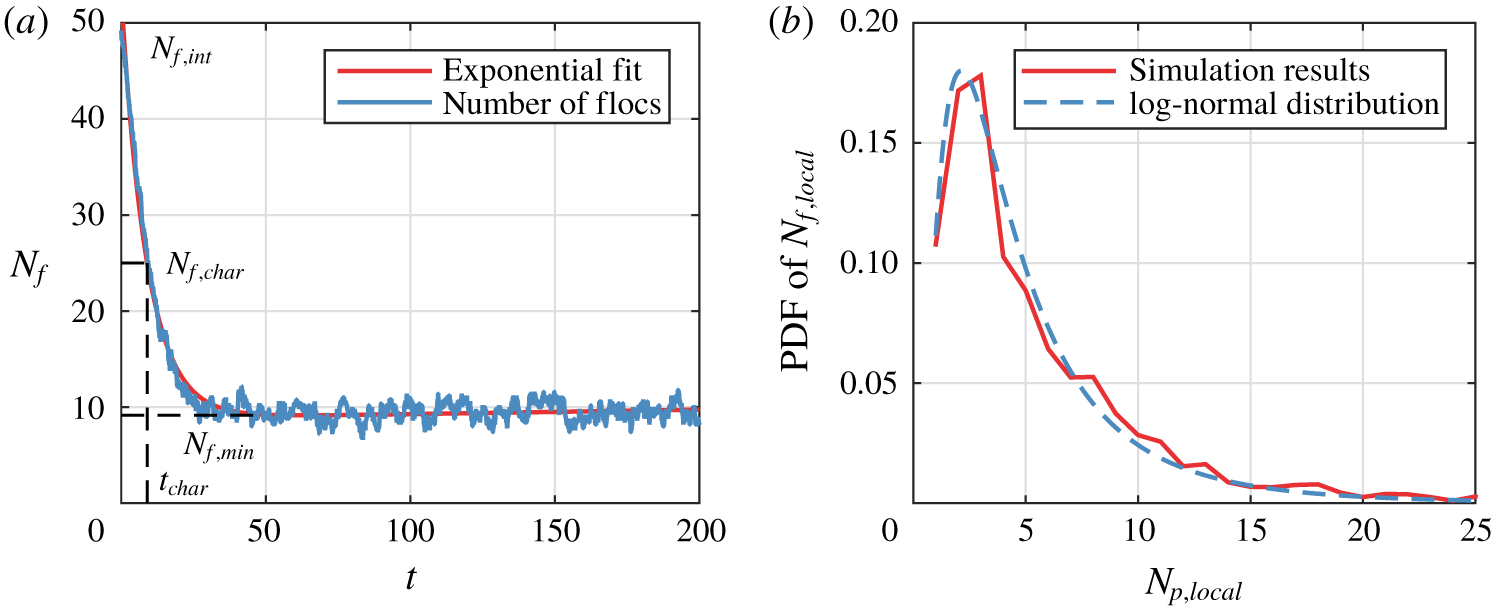
(a) Typical evolution of the number of flocs  $N_{f}$ as function of time; and (b) floc size distribution during the equilibrium stage
 $50\leqslant t\leqslant 200$. Simulation parameters are
 $N_{p}=50$,
 $D_{p}=0.1$,
 $\unicode[STIX]{x1D70C}_{s}=1$,
 $W=0$,
 $St=0.1$ and
 $Co=5\times 10^{-4}$. PDF, probability density function.

A typical floc configuration is shown in figure 1(b). Figure 3(a) presents results for a series of simulations with  $N_{p}=50$ particles that have a size of 10 % of the Kolmogorov length scale, i.e.
 $D_{p}=0.1$. Further, the parameters for this scenario were
 $\unicode[STIX]{x1D70C}_{s}=1$,
 $W=0$,
 $St=0.1$ and
 $Co=5\times 10^{-4}$. Since the particles are dispersed initially, the initial number of flocs
 $N_{f,int}\approx N_{p}$. Subsequently
 $N_{f}$ decreases rapidly due to flocculation, before levelling off around a constant value
 $N_{f,min}$ that reflects a stable balance between aggregation and breakage. The transient variation of
 $N_{f}(t)$ can be fitted by an exponential function of the form
 $$\begin{eqnarray}N_{f}=(N_{f,int}-N_{f,min})\text{e}^{bt}+N_{f,min},\end{eqnarray}$$
where we evaluate  $N_{f,min}$ as the average number of flocs during the equilibrium stage
 $50\leqslant t\leqslant 200$. The agglomeration rate
 $\left|b\right|$ with the constraint
 $b\leqslant 0$ is obtained via a least-squares fit. We define the characteristic flocculation time scale
 $t_{char}$ as the time it takes for the number of flocs to decrease from its initial value
 $N_{f,int}$ to a characteristic number of flocs
 $N_{f,char}=N_{p}/2$. Hence the corresponding characteristic time can be calculated as
 $t_{char}=\text{ln}[(N_{p}/2-N_{f,min})/(N_{f,int}-N_{f,min})]/b$.
Figure 3(b) displays the statistical floc size distribution during the equilibrium stage  $50\leqslant t\leqslant 200$, where the ‘floc size’
 $N_{p,local}$ denotes the number of particles in a floc. Here
 $N_{f,local}$ refers to the number of the flocs of the same size. We find that the floc size distribution closely follows a log-normal distribution, consistent with previous experimental observations (Bouyer, Line & Do-quang Reference Bouyer, Line and Do-quang2004; Hill et al. Reference Hill, Boss, Newgard, Law and Milligan2011; Verney et al. Reference Verney, Lafite, Burn-Cottan and le Hir2011).
3.2 Influence of the governing parameters on the flocculation dynamics
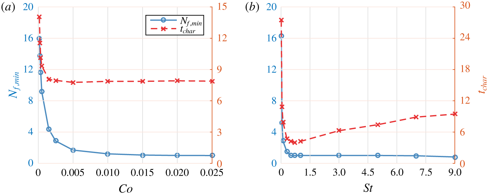
In order to explore the dependence of the flocculation process on the key governing quantities, we carry out a total of 300 simulations covering the parameter ranges listed in table 1. Figure 4(a) shows that the number of flocs during the equilibrium stage  $N_{f,min}$ decreases for increasing
 $Co$. Beyond
 $Co\approx 0.01$, all of the primary particles aggregate into one large floc, as the cohesive forces overwhelm the hydrodynamic stresses trying to break up the floc. The characteristic flocculation time initially decreases as
 $Co$ grows, and then levels off and remains constant. Figure 4(b) indicates that for large Stokes numbers,
 $St$, the equilibrium floc number,
 $N_{f,min}$, also asymptotically approaches one. Interestingly, we observe that the flocculation time
 $t_{char}$ displays a pronounced minimum around
 $St\approx 0.7$, which reflects the well-known optimal coupling between particle and fluid motion when the particle response time is of the same order as the characteristic time scale of the flow (Wang & Maxey Reference Wang and Maxey1993). Under these conditions, particles rapidly accumulate near the edges of the vortices, which facilitates the formation of flocs.
The flocculation time scale and the equilibrium number of flocs as functions of  $Co$ and
 $St$, respectively, for
 $N_{p}=50$,
 $D_{p}=0.1$,
 $\unicode[STIX]{x1D70C}_{s}=1$ and
 $W=0$: (a) influence of the cohesive number
 $Co$, for
 $St=0.1$; (b) influence of the Stokes number
 $St$, for
 $Co=2.5\times 10^{-3}$.

Simulated parameter ranges. The particle number  $N_{p}$ is converted into the pseudo volume fraction
 $\unicode[STIX]{x1D719}=(\unicode[STIX]{x03C0}N_{p}D_{p}^{3})/(6L_{x}L_{y}D_{p})$. Note that
 $D_{p}$ is a dimensionless value normalized by the characteristic length scale
 $L$.

3.3 A new flocculation model based on the simulation data
According to Khelifa & Hill (Reference Khelifa and Hill2006a,Reference Khelifa and Hillb), for flocs of fractal dimension  $n_{f}$ the mean floc size
 $\overline{D}_{f}$ is related to the average number of primary particles per floc
 $\overline{N}_{p,local}=N_{p}/N_{f}$:
 $$\begin{eqnarray}\overline{D}_{f}=(\overline{N}_{p,local})^{1/n_{f}}D_{p}.\end{eqnarray}$$
Equation (3.1) yields for the average number of particles per floc
 $$\begin{eqnarray}\overline{N}_{p,local}={\displaystyle \frac{1}{(1/\overline{N}_{p,local,int}-1/\overline{N}_{p,local,max})\text{e}^{bt}+1/\overline{N}_{p,local,max}}},\end{eqnarray}$$
where the initial number of particles per floc is  $\overline{N}_{p,local,int}=N_{p}/N_{f,int}$, and the average number of particles per floc during the equilibrium stage is
 $\overline{N}_{p,local,max}=N_{p}/N_{f,min}$. Fitting the simulation results over the parameter ranges listed in table 1 yields
 $$\begin{eqnarray}\displaystyle & \displaystyle \overline{N}_{p,local,max}=8.5a_{1}St^{0.65}Co^{0.58}D_{p}^{-2.9}\unicode[STIX]{x1D719}^{0.39}\unicode[STIX]{x1D70C}_{s}^{-0.49}(W+1)^{-0.38}, & \displaystyle\end{eqnarray}$$
 $$\begin{eqnarray}\displaystyle & \displaystyle \overline{N}_{p,local,max}=N_{p},\quad \text{ if }\overline{N}_{p,local,max}\geqslant N_{p}, & \displaystyle\end{eqnarray}$$
 $$\begin{eqnarray}b=\left\{\begin{array}{@{}ll@{}}-0.7a_{2}St^{0.36}Co^{-0.017}D_{p}^{-0.36}\unicode[STIX]{x1D719}^{0.75}\unicode[STIX]{x1D70C}_{s}^{-0.11}(W+1)^{-1.4}, & St\leqslant 0.7,\\ -0.3a_{2}St^{-0.38}Co^{0.0022}D_{p}^{-0.61}\unicode[STIX]{x1D719}^{0.67}\unicode[STIX]{x1D70C}_{s}^{0.033}(W+1)^{-0.46}, & St>0.7.\end{array}\right.\end{eqnarray}$$
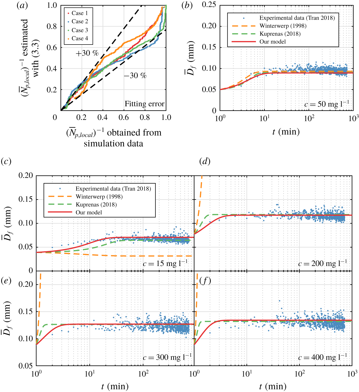
For the present cellular model flow the values  $a_{1}=a_{2}=1$ in (3.4a) and (3.5) yield optimal agreement with the simulation data with the fitting deviation of
 $\pm 30\,\%$ (figure 5a). For real turbulent flows, we will determine
 $a_{1}$ and
 $a_{2}$ by calibrating with experimental data, as will be explained below.
Winterwerp (Reference Winterwerp1998) introduced a population balance model that accounts for aggregation and breakage for low turbulence levels. His model has the form
 $$\begin{eqnarray}{\displaystyle \frac{\text{d}\overline{D}_{f}}{\text{d}t}}={\displaystyle \frac{k_{A}^{\prime }}{n_{f}}}{\displaystyle \frac{D_{p}^{n_{f}-3}}{\unicode[STIX]{x1D70C}_{p}}}Gc\overline{D}_{f}^{4-n_{f}}-{\displaystyle \frac{k_{B}^{\prime }}{n_{f}}}\left({\displaystyle \frac{\unicode[STIX]{x1D707}_{f}}{F_{y}}}\right)^{q}\left({\displaystyle \frac{\overline{D}_{f}-D_{p}}{D_{p}}}\right)^{p}G^{q+1}\overline{D}_{f}^{2q+1},\end{eqnarray}$$
where  $G$ indicates the shear rate of the turbulence (units
 $\text{s}^{-1}$),
 $c$ represents the sediment concentration (
 $\text{kg}~\text{m}^{-3}$), and
 $F_{y}$ denotes the yield strength of the flocs (N). Winterwerp suggests the values
 $F_{y}=10^{-10}~\text{N}$,
 $n_{f}=2$,
 $p=1$ and
 $q=0.5$. The empirical coefficients
 $k_{A}^{\prime }$ and
 $k_{B}^{\prime }$ depend on the physico-chemical properties of the sediment and fluid. While this model has enjoyed wide popularity in the literature (Winterwerp et al. Reference Winterwerp, Manning, Martens, de Mulder and Vanlede2006; Son & Hsu Reference Son and Hsu2008, Reference Son and Hsu2009; Lee et al. Reference Lee, Toorman, Molz and Wang2011; Keyvani & Strom Reference Keyvani and Strom2014; Strom & Keyvani Reference Strom and Keyvani2016), it has also been pointed out that for large turbulent shear and sediment concentrations the model predicts that the floc size will be larger than the Kolmogorov scale
 $\unicode[STIX]{x1D702}$, which is not consistent with experimental observations (Keyvani & Strom Reference Keyvani and Strom2014; Kuprenas, Tran & Strom Reference Kuprenas, Tran and Strom2018; Sherwood, Aretxabaleta & Harris Reference Sherwood, Aretxabaleta and Harris2018). To address this issue, Kuprenas et al. (Reference Kuprenas, Tran and Strom2018) recently suggested the modification
 $q=0.5+1.5\overline{D}_{f}/\unicode[STIX]{x1D702}$. In the following, we will compare predictions by the current model with both of these earlier models.
(a) Total fitting deviation of (3.3)–(3.5), cases 1 to 4 shown here have the largest fitting error among 300 different tests for the cellular flow field (figure 1a). Comparison with experimental data: (b) calibration of the empirical coefficients for the models of Winterwerp (Reference Winterwerp1998) ( $k_{A}^{\prime }=1.35$ and
 $k_{B}^{\prime }=1.29\times 10^{-5}$), Kuprenas et al. (Reference Kuprenas, Tran and Strom2018) (
 $k_{A}^{\prime }=0.45$ and
 $k_{B}^{\prime }=1.16\times 10^{-6}$), and for our (3.4)–(3.5) (
 $a_{1}=500$ and
 $a_{2}=35$); (c–f) comparisons between experimental data and predictions by the model of Kuprenas et al. (Reference Kuprenas, Tran and Strom2018) and (3.2)–(3.5); the predictions by Winterwerp (Reference Winterwerp1998) are also shown for further comparison. The experimental parameters are
 $D_{p}=5~\unicode[STIX]{x03BC}\text{m}$,
 $G=50~\text{s}^{-1}$,
 $\unicode[STIX]{x1D70C}_{p}=2650~\text{kg}~\text{m}^{-3}$,
 $\unicode[STIX]{x1D70C}_{f}=1000~\text{kg}~\text{m}^{-3}$,
 $\unicode[STIX]{x1D707}_{f}=0.001~\text{Ns}~\text{m}^{-2}$,
 $c=15\sim 400~\text{mg}~\text{l}^{-1}$.

Tran, Kuprenas & Strom (Reference Tran, Kuprenas and Strom2018) measured the floc size  $\overline{D}_{f}(t)$ in turbulence for constant shear rate
 $G$ and sediment concentration
 $c$ (figure 5b–f). They determined the empirical coefficients
 $k_{A}^{\prime }$ and
 $k_{B}^{\prime }$ by calibrating with the experimental data for
 $c=50~\text{mg}~\text{l}^{-1}$. In a similar fashion, we will determine the constants
 $a_{1}$ and
 $a_{2}$ required for our model by calibrating with the same case displayed in figure 5(b). Towards this end, we need to convert the experimental data into characteristic length
 $L$ and velocity
 $U_{0}$ scales that can be employed in our model – equations (3.3)–(3.5). We accomplish this by setting
 $L=\unicode[STIX]{x1D702}=[\unicode[STIX]{x1D707}_{f}/(\unicode[STIX]{x1D70C}_{f}G)]^{0.5}$ and
 $U_{0}=G\unicode[STIX]{x1D702}/4$. Furthermore, we assume the Hamaker constant to be
 $A_{H}=1.0\times 10^{-20}~\text{J}$ (see Vowinckel et al. Reference Vowinckel, Withers, Luzzatto-Fegiz and Meiburg2019, pp. 37–39), and the fractal dimension
 $n_{f}=2$, which yields the correction constants
 $a_{1}=500$ and
 $a_{2}=35$. The mean floc size can then be obtained from (3.2). For lower sediment loadings, figure 5(c) shows that our model yields predictions similar to those of Kuprenas for the equilibrium floc size, while it tends to perform somewhat better than Kuprenas’ model during the transient stage. These differences become more pronounced for higher sediment loadings (figure 5d–f), and they likely reflect the more realistic modelling of the particle–particle interactions in the present simulations. For these particular flow conditions, Winterwerp’s model yields valid predictions only for sediment loads below approximately
 $200~\text{mg}~\text{l}^{-1}$. Hence, the results encourage the use of our conceptually simplified cellular flow model as a cost-efficient tool to derive scaling laws in the form of (3.2)–(3.5) for a wide parameter range for flocculation of cohesive particles in turbulent flow conditions.
4 Conclusions
We have analysed the flocculation dynamics of cohesive sediment via one-way coupled simulations in a model turbulent flow field. The computational model accounts for Stokes drag, lubrication, cohesive and direct contact forces, and it yields the time-dependent floc size as a function of the governing dimensionless parameters. The simulations reproduce the transient growth of the cohesive flocs, as well as the emergence of a log-normal equilibrium distribution governed by the balance of aggregation and breakage. By accounting for the detailed physical mechanisms governing particle–particle interactions, the simulations demonstrate that flocculation proceeds most rapidly when the Stokes number of the primary particles is O (1). We employ the computational data in order to propose a new flocculation model. As it is based on a more realistic representation of particle–particle interactions, this new model yields improved agreement with the experimental measurements of Tran et al. (Reference Tran, Kuprenas and Strom2018), especially during the transient stages.
Acknowledgements
The authors thank D. Tran for providing his experimental data for comparison purposes. E.M. gratefully acknowledges support through NSF grants CBET-1803380 and OCE-1924655, as well as by the Army Research Office through grant W911NF-18-1-0379. T.-J.H. received support through NSF grant OCE-1924532. K.Z. is supported by the China Scholarship Council, as well as by the China National Fund for Distinguished Young Scientists through grant 51425603. B.V. gratefully acknowledges support through German Research Foundation (DFG) grant VO2413/2-1. Computational resources for this work used the Extreme Science and Engineering Discovery Environment (XSEDE), which is supported by NSF grant TG-CTS150053.