


1 Introduction
Accurate prediction of water levels in rough-bed open-channel flows (OCFs) is probably among the oldest hydraulic problems that still await proper solutions. Despite significant efforts to advance this subject matter, hydraulic engineers continue to use empirical or semi-empirical approaches utilising Manning’s
 $n=R^{2/3}S_{b}^{1/2}/U$
, Chezy’s
 $C=U/(RS_{b})^{1/2}$
, or the Darcy–Weisbach
 $f_{cs}=8\unicode[STIX]{x1D70F}_{0cs}/(\unicode[STIX]{x1D70C}U^{2})$
resistance coefficients (e.g. Graf & Altinakar Reference Graf and Altinakar1998), where
 $U$
is cross-sectionally averaged velocity;
 $R$
is hydraulic radius, which for two-dimensional flow is equivalent to the mean flow depth;
 $S_{b}$
is mean bed slope;
 $\unicode[STIX]{x1D70C}$
is fluid density; and
 $\unicode[STIX]{x1D70F}_{0cs}$
is bed shear stress averaged over the whole cross-section. These resistance coefficients represent the combined effects of complex hydrodynamic processes in simple forms, making them convenient for practical applications based on cross-sectionally averaged hydraulic models. Although Manning’s
 $n$
, Chezy’s
 $C$
and the Darcy–Weisbach
 $f_{cs}$
are interrelated (i.e.
 $f_{cs}=8gn^{2}/R^{1/3}=8g/C^{2}$
, where
 $g$
denotes gravity acceleration), there is a growing consensus that for hydraulic applications the Darcy–Weisbach friction factor is generally preferable. In addition to the cross-sectional
 $f_{cs}$
, researchers and engineers have increasingly used a ‘local’ friction factor
 $f=8\unicode[STIX]{x1D70F}_{0}/(\unicode[STIX]{x1D70C}\widehat{U}^{2})$
characterising bed friction
 $\unicode[STIX]{x1D70F}_{0}$
at a particular transverse location and thus suitable for depth-averaged hydraulic models (e.g. Morvan et al.
Reference Morvan, Knight, Wright, Tang and Crossley2008), where
 $\widehat{U}$
is a depth-averaged velocity. Following this trend, all considerations in our paper relate to this ‘local’ friction factor
 $f$
. In the next section we will show that the Darcy–Weisbach friction factor
 $f$
may be presented as a sum of contributions from specific resistance-forming mechanisms, providing an additional reason for using it in hydraulic applications.
There is a general agreement that resistance coefficients for OCFs depend on the flow parameters (e.g. Reynolds number, Froude number, relative submergence, turbulent stresses, secondary currents, non-uniformity/unsteadiness), bed material (e.g. bed particle shape and dimensions), bed forms (e.g. steepness), plane channel forms (e.g. channel sinuosity) and in-stream vegetation (e.g. plant geometry, areal density and biomechanics). Although the quantitative forms of these dependences have been targeted by several generations of hydraulicians, available relationships linking the resistance coefficients to flow and roughness parameters are still largely empirical, rather than rigorously justified (e.g. Yen Reference Yen2002). As a result, the level of uncertainties in cross-sectionally averaged, depth-averaged and three-dimensional hydraulic models of overland flows, canals, rivers, estuaries and other free-surface flows remains high, often exceeding 20–40 % (e.g. Yen Reference Yen2002; Knight et al. Reference Knight, Hazlewood, Lamb, Samuels and Shiono2018). This state of affairs motivates new research efforts that should lead to better justified friction factor equations.
The potential options for the rigorous derivation of the friction factor equation unavoidably start with the conventional Navier–Stokes equation (or its various forms) combined with an appropriate physical interpretation of the friction factor as a similarity number. Traditionally, the friction factor is interpreted as the ratio of the drag forces at the bed to the inertial forces. Equivalently, the friction factor can be also viewed as the ratio of the rate of momentum sink at the bed surface (
 $\unicode[STIX]{x1D70F}_{0}$
) to the bulk streamwise flux of momentum (
 $\unicode[STIX]{x1D70C}\widehat{U}^{2}$
). This way, an expression for the friction factor can be obtained through appropriate integration of the Navier–Stokes equation that would involve a few steps for obtaining the bed shear stress, local velocity (at a point in the flow) and, finally, the ratio of the bed shear stress to the squared bulk velocity (times fluid density
 $\unicode[STIX]{x1D70C}$
), i.e.
 $f=8\unicode[STIX]{x1D70F}_{0}/(\unicode[STIX]{x1D70C}\widehat{U}^{2})$
. Such a momentum-based approach was followed, essentially, by Fukagata, Iwamoto & Kasagi (Reference Fukagata, Iwamoto and Kasagi2002) who proposed, for the first time, an explicit decomposition of the friction factor for hydraulically smooth-wall boundary layers, closed channels and pipes. Fukagata et al.’s (Reference Fukagata, Iwamoto and Kasagi2002) approach has been subsequently expanded to cover three-dimensional flows over walls of complex geometry (Peet & Sagaut Reference Peet and Sagaut2009; Bannier, Garnier & Sagaut Reference Bannier, Garnier and Sagaut2015). Recently, two complementary decompositions have been suggested, also for smooth-wall flows, based on the mean energy balance (Renard & Deck Reference Renard and Deck2016) and mean vorticity equation (Yoon et al.
Reference Yoon, Ahn, Hwang and Sung2016).
Renard & Deck’s (Reference Renard and Deck2016) approach adopts, tacitly, a less conventional interpretation of the friction factor as the ratio of the power of the surface forces at the bed (
 $\widehat{U}\unicode[STIX]{x1D70F}_{0}$
) to the bulk flow power (
 $\unicode[STIX]{x1D70C}\widehat{U}^{3}$
) and employs, accordingly, the mean kinetic energy budget. The energy approach is physically appealing and may provide additional insights into friction mechanisms and in interpretation of long-established relations such as resistance equations. Recently, for example, Abe & Antonia (Reference Abe and Antonia2016) employed an energy-based expression
 $\unicode[STIX]{x1D700}H/u_{\ast }^{3}\propto (1/f)^{1/2}$
, where
 $u_{\ast }=(\unicode[STIX]{x1D70F}_{0}/\unicode[STIX]{x1D70C})^{0.5}$
is shear velocity and
 $\unicode[STIX]{x1D700}$
is energy dissipation. They demonstrated that good performance of the logarithmic skin friction equation at fairly low Reynolds number is a result of the logarithmic scaling of the energy dissipation rather than a signature of the logarithmic velocity profile. Yoon et al.’s (Reference Yoon, Ahn, Hwang and Sung2016) approach is based on the presentation of the velocity derivative
 $\unicode[STIX]{x2202}\overline{u}/\unicode[STIX]{x2202}z$
in the equation for the wall shear stress
 $\unicode[STIX]{x1D70F}_{0}=\unicode[STIX]{x1D70C}\unicode[STIX]{x1D708}(\unicode[STIX]{x2202}\overline{u}/\unicode[STIX]{x2202}z)|_{z=0}$
using the spanwise component of the mean vorticity
 $\unicode[STIX]{x1D6FA}_{y}=\unicode[STIX]{x2202}\overline{w}/\unicode[STIX]{x2202}x-\unicode[STIX]{x2202}\overline{u}/\unicode[STIX]{x2202}z$
, leading to
 $\unicode[STIX]{x1D70F}_{0}=\unicode[STIX]{x1D70C}\unicode[STIX]{x1D708}(\unicode[STIX]{x2202}\overline{u}/\unicode[STIX]{x2202}z)|_{z=0}=\unicode[STIX]{x1D70C}\unicode[STIX]{x1D708}(\unicode[STIX]{x2202}\overline{w}/\unicode[STIX]{x2202}x-\unicode[STIX]{x1D6FA}_{y})|_{z=0}$
(
 $\unicode[STIX]{x1D708}$
is fluid kinematic viscosity,
 $\overline{u}$
and
 $\overline{w}$
are Reynolds-averaged streamwise and vertical velocities,
 $z$
and
 $x$
are vertical and streamwise coordinates). This re-arrangement allowed Yoon et al. (Reference Yoon, Ahn, Hwang and Sung2016) to employ the mean vorticity equation, which after triple integration produced an expression for the friction factor linking it to velocity–vorticity correlations. The vorticity-based approach is also physically interesting and instructive but the similarity meaning of the friction factor in the form of
 $f=\unicode[STIX]{x1D708}(\unicode[STIX]{x2202}\overline{w}/\unicode[STIX]{x2202}x-\unicode[STIX]{x1D6FA}_{y})|_{z=0}/\widehat{U}^{2}$
is less clear.
For the case of rough-bed flows the available approaches are not straightforward to apply as they do not account for the roughness-scale flow separations and emergence of the associated pressure drag at the bed. As an example, the vorticity-based interpretation of the friction factor
 $f=\unicode[STIX]{x1D708}(\unicode[STIX]{x2202}\overline{w}/\unicode[STIX]{x2202}x-\unicode[STIX]{x1D6FA}_{y})|_{z=0}/\widehat{U}^{2}$
is possible only if the pressure drag at roughness elements is completely absent. For our considerations of rough-bed open-channel flows we have chosen the momentum-based approach, as our focus is on the identification and quantification of the key momentum transport mechanisms leading to the momentum sink (or drag) at the bed. A preliminary derivation of our momentum-based approach for rough-bed OCFs is outlined in Nikora (Reference Nikora2009) and will be refined below in § 2.
The key objectives of the present paper are: (i) to propose a decomposition of the friction factor, which is suitable for both smooth-bed and rough-bed OCFs and thus can be viewed as a generalisation of Fukagata et al.’s (Reference Fukagata, Iwamoto and Kasagi2002) momentum-based approach, initially proposed for smooth-wall flows; (ii) based on this decomposition, to evaluate contributions of viscous, turbulent and dispersive (due to bed roughness and secondary currents) stresses to bed friction for self-affine isotropic rough boundaries resembling natural and man-made roughness types; and (iii) to assess the effects of bed roughness type, Reynolds number and relative submergence on mechanism-specific contributions to the overall friction factor. The required data for the study are provided by a series of high-precision laboratory experiments and complementary large-eddy simulations (LES), specifically designed and conducted to support this work. Although the reported methodology and findings relate to OCFs, they are also relevant to other types of rough-wall-bounded flows (boundary layers, conduits, pipes), at least conceptually.
2 Friction factor decomposition for rough-bed flows
2.1 Theoretical background
The derivation of a general relationship for the friction factor for fixed- and mobile-rough-bed flows starts with the double-averaged (in time and in volume of a thin slab parallel to the bed) momentum equation proposed in Nikora et al. (Reference Nikora, Ballio, Coleman and Pokrajac2013). Here, for simplicity (but without losing conceptual generality) we consider a simpler case of fixed-rough-bed OCF for which the double-averaged momentum equation for the streamwise velocity component can be written as
 $$\begin{eqnarray}\displaystyle \frac{\unicode[STIX]{x2202}\langle \overline{u}_{1}\rangle }{\unicode[STIX]{x2202}t}+\langle \overline{u}_{j}\rangle \frac{\unicode[STIX]{x2202}\langle \overline{u}_{1}\rangle }{\unicode[STIX]{x2202}x_{j}} & = & \displaystyle gS_{b}-\frac{1}{\unicode[STIX]{x1D70C}\unicode[STIX]{x1D719}}\frac{\unicode[STIX]{x2202}\unicode[STIX]{x1D719}\langle \overline{p}\rangle }{\unicode[STIX]{x2202}x_{1}}-\frac{1}{\unicode[STIX]{x1D719}}\frac{\unicode[STIX]{x2202}\unicode[STIX]{x1D719}\langle \overline{u_{1}^{\prime }u_{j}^{\prime }}\rangle }{\unicode[STIX]{x2202}x_{j}}-\frac{1}{\unicode[STIX]{x1D719}}\frac{\unicode[STIX]{x2202}\unicode[STIX]{x1D719}\langle \widetilde{\overline{u}}_{1}\widetilde{\overline{u}}_{j}\rangle }{\unicode[STIX]{x2202}x_{j}}+\frac{1}{\unicode[STIX]{x1D719}}\frac{\unicode[STIX]{x2202}}{\unicode[STIX]{x2202}x_{j}}\unicode[STIX]{x1D719}\left\langle \overline{\unicode[STIX]{x1D708}\frac{\unicode[STIX]{x2202}u_{1}}{\unicode[STIX]{x2202}x_{j}}}\right\rangle \nonumber\\ \displaystyle & & \displaystyle -\,\frac{1}{V_{f}}\iint _{S_{int}}\unicode[STIX]{x1D708}\frac{\unicode[STIX]{x2202}\overline{u}_{1}}{\unicode[STIX]{x2202}x_{j}}m_{j}\text{d}S+\frac{1}{\unicode[STIX]{x1D70C}}\frac{1}{V_{f}}\iint _{S_{int}}\overline{p}m_{1}\text{d}S.\end{eqnarray}$$
In (2.1), the Reynolds decomposition
 $\unicode[STIX]{x1D703}=\overline{\unicode[STIX]{x1D703}}+\unicode[STIX]{x1D703}^{\prime }$
for instantaneous variables and the decomposition
 $\overline{\unicode[STIX]{x1D703}}=\langle \overline{\unicode[STIX]{x1D703}}\rangle +\widetilde{\overline{\unicode[STIX]{x1D703}}}$
for time-averaged variables are used where
 $\unicode[STIX]{x1D703}$
is a flow variable (i.e. velocity or pressure) defined in the fluid but not in the space occupied by the roughness elements; angle brackets denote spatial (volume) averaging, overbar denotes time averaging and prime and tilde denote temporally and spatially fluctuating components, respectively;
 $u_{i}$
is the
 $i$
th component of the velocity vector;
 $p$
is pressure;
 $m_{i}$
is a unit vector normal to the bed surface and directed into the fluid;
 $S_{int}$
is the extent of water–bed interface bounded by the averaging domain;
 $\unicode[STIX]{x1D719}=V_{f}/V_{0}$
is the roughness geometry function or ‘spatial porosity’ (Nikora et al.
Reference Nikora, Goring, McEwan and Griffiths2001), where
 $V_{f}$
is volume occupied by fluid within the averaging domain of the total volume
 $V_{0}$
; and
 $x_{1}=x$
(streamwise),
 $x_{2}=y$
(spanwise),
 $x_{3}=z$
(bed normal) are orthogonal coordinates. In wall-bounded flows such as rivers, there are strong gradients in flow properties in the wall-normal direction, especially near the bed, and therefore the volume-averaging domain should be a thin slab parallel to the mean bed. The dimensions of the averaging domain in the plane parallel to the mean bed define a scale of consideration and should typically exceed relevant correlation length scales of bed roughness. Thus, the double-averaged quantities in (2.1) depend, in general, on all three spatial coordinates (
 $x$
,
 $z$
and
 $y$
) and time
 $t$
, considering length and time scales well exceeding characteristic scales of bed roughness and turbulence, respectively (Nikora et al.
Reference Nikora, McEwan, McLean, Coleman, Pokrajac and Walters2007). For simplicity, however, we will omit the explicit indication (
 $x$
,
 $y$
,
 $z$
,
 $t$
) of this dependency, presenting double-averaged quantities
 $\langle \overline{u}_{i}\rangle (x,y,z,t)$
,
 $\langle \overline{p}\rangle (x,y,z,t)$
,
 $\langle \overline{u_{i}^{\prime }u_{j}^{\prime }}\rangle (x,y,z,t)$
and
 $\langle \widetilde{\overline{u}}_{i}\widetilde{\overline{u}}_{j}\rangle (x,y,z,t)$
as
 $\langle \overline{u}_{i}\rangle$
,
 $\langle \overline{p}\rangle$
,
 $\langle \overline{u_{i}^{\prime }u_{j}^{\prime }}\rangle$
and
 $\langle \widetilde{\overline{u}}_{i}\widetilde{\overline{u}}_{j}\rangle$
. Compared to the conventional ensemble-(time-) averaged momentum equation, (2.1) contains two groups of additional terms: (i) dispersive stresses
 $\langle \widetilde{\overline{u}}_{i}\widetilde{\overline{u}}_{j}\rangle$
due to potential correlations of spatial variations in time-averaged velocity fields (also known as form-induced stresses); and (ii) viscous drag per unit fluid volume
 $\unicode[STIX]{x1D6F7}_{\unicode[STIX]{x1D708}}=(1/V_{f})\iint _{S_{int}}(\unicode[STIX]{x1D70C}\unicode[STIX]{x1D708}\unicode[STIX]{x2202}\overline{u}_{1}/\unicode[STIX]{x2202}x_{j})m_{j}\text{d}S$
and form (pressure) drag per unit fluid volume
 $\unicode[STIX]{x1D6F7}_{p}=-(1/V_{f})\iint _{S_{int}}\overline{p}m_{1}\text{d}S$
, which together define the total drag per unit volume
 $F_{D}=\unicode[STIX]{x1D719}(\unicode[STIX]{x1D6F7}_{\unicode[STIX]{x1D708}}+\unicode[STIX]{x1D6F7}_{p})$
(e.g. Nikora et al.
Reference Nikora, McEwan, McLean, Coleman, Pokrajac and Walters2007, Reference Nikora, Ballio, Coleman and Pokrajac2013). The development of the double-averaged hydrodynamic equations for rough-bed flows was initiated by atmospheric scientists for describing turbulent flows within and above terrestrial canopies such as forests or bushes (Wilson & Shaw Reference Wilson and Shaw1977; Raupach & Shaw Reference Raupach and Shaw1982; Finnigan Reference Finnigan2000) and later this approach was adopted in studies of rough-bed open-channel flows.
In a first step of derivation, (2.1) is appropriately re-arranged and integrated from the roughness troughs
 $z_{t}$
to the water surface
 $z_{ws}$
, to obtain an equation that explicitly involves the local bed shear stress
 $\unicode[STIX]{x1D70F}_{0}$
, defined here as
 $$\begin{eqnarray}\displaystyle \unicode[STIX]{x1D70F}_{0}=\int _{z_{t}}^{z_{c}}\frac{1}{V_{0}}\left[\iint _{S_{int}}\left(\unicode[STIX]{x1D70C}\unicode[STIX]{x1D708}\frac{\unicode[STIX]{x2202}\overline{u}_{1}}{\unicode[STIX]{x2202}x_{j}}\right)m_{j}\,\text{d}S-\iint _{S_{int}}\overline{p}m_{1}\,\text{d}S\right]\text{d}z=\int _{z_{t}}^{z_{c}}F_{D}\,\text{d}z, & & \displaystyle\end{eqnarray}$$
where
 $z_{c}$
is the elevation of the roughness crests. Then, a triple integration
 $\int _{z_{t}}^{z_{ws}}\text{d}z\int _{z_{t}}^{z}\text{d}z\int _{z_{t}}^{z}\text{d}z$
is applied to the difference between (2.1) and the obtained equation, similar to Fukagata et al.’s (Reference Fukagata, Iwamoto and Kasagi2002) procedure for smooth-bed flows. The first two integrations are required to obtain an explicit equation for the local double-averaged velocity
 $\langle \overline{u}_{1}\rangle$
while the third integration over the flow depth gives a depth-averaged velocity
 $\widehat{U}=H^{-1}\int _{z_{t}}^{z_{ws}}\unicode[STIX]{x1D719}\langle \overline{u}_{1}\rangle \,\text{d}z$
, where
 $H$
is the mean flow depth, defined as
 $H=\int _{z_{t}}^{z_{ws}}\unicode[STIX]{x1D719}\,\text{d}z=z_{ws}-z_{c}+\int _{z_{t}}^{z_{c}}\unicode[STIX]{x1D719}\,\text{d}z$
. As follows from this definition, the depth-averaged velocity
 $\widehat{U}$
and ‘local’ friction factor
 $f=8\unicode[STIX]{x1D70F}_{0}/(\unicode[STIX]{x1D70C}\widehat{U}^{2})$
may depend, in general, on the streamwise and transverse coordinates and time (at time scales well exceeding turbulent scales and at length scales well exceeding roughness scales). For steady, uniform, and two-dimensional flow (in the double-averaged sense) these quantities do not depend on spatial coordinates and time.
Subsequent re-arrangement of the integrated equation leads to the following decomposition of the friction factor
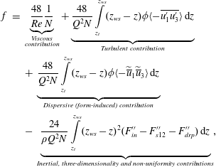
where the Reynolds number is defined as
 $Re=\widehat{U}H/\unicode[STIX]{x1D708}$
;
 $Q=\widehat{U}H$
is a specific flow rate (i.e. per unit width);
 $N=3(L_{\unicode[STIX]{x1D70F}}/H)^{2}+(\unicode[STIX]{x1D70F}_{02D}/\unicode[STIX]{x1D70F}_{0})(L_{\unicode[STIX]{x1D719}}/H)^{3}-(H_{m}/H)^{3}$
is a parameter characterising flow–rough-bed interactions;
 $\unicode[STIX]{x1D70F}_{02D}=\unicode[STIX]{x1D70C}gS_{b}H$
is the bed shear stress that would act if the flow was steady, two-dimensional (2-D) and uniform in terms of the double-averaged quantities (Nikora et al.
Reference Nikora, McEwan, McLean, Coleman, Pokrajac and Walters2007);
 $H_{m}$
is the maximum flow depth, i.e.
 $H_{m}=z_{ws}-z_{t}$
;
 $L_{\unicode[STIX]{x1D70F}}$
is a ‘drag’ length scale,
 $L_{\unicode[STIX]{x1D70F}}=(\int _{z_{t}}^{z_{c}}(z_{ws}-z)^{2}F_{D}\,\text{d}z/\int _{z_{t}}^{z_{c}}F_{D}\,\text{d}z)^{0.5}$
with
 $\int _{z_{t}}^{z_{c}}F_{D}\,\text{d}z=\unicode[STIX]{x1D70F}_{0}$
;
 $L_{\unicode[STIX]{x1D719}}$
is a ‘depth-roughness’ length scale,
 $L_{\unicode[STIX]{x1D719}}=(3\int _{z_{t}}^{z_{ws}}(z_{ws}-z)^{2}(1-\unicode[STIX]{x1D719})\,\text{d}z)^{1/3}$
; and
 $F_{in}^{\prime \prime }$
,
 $F_{s12}^{\prime \prime }$
and
 $F_{drp}^{\prime \prime }$
represent deviations of the inertial force (
 $F_{in}^{\prime \prime }$
), fluid forces in the
 $x$
–
 $y$
plane (
 $F_{s12}^{\prime \prime }$
) and pressure force (
 $F_{drp}^{\prime \prime }$
) per unit volume from their depth-averaged counterparts, i.e.
 $$\begin{eqnarray}\displaystyle F_{in}^{\prime \prime } & = & \displaystyle \unicode[STIX]{x1D70C}\unicode[STIX]{x1D719}\left(\frac{\unicode[STIX]{x2202}\langle \overline{u}_{1}\rangle }{\unicode[STIX]{x2202}t}+\langle \overline{u}_{j}\rangle \frac{\unicode[STIX]{x2202}\langle \overline{u}_{1}\rangle }{\unicode[STIX]{x2202}x_{j}}\right)-\frac{1}{H}\int _{z_{t}}^{z_{ws}}\unicode[STIX]{x1D70C}\unicode[STIX]{x1D719}\left(\frac{\unicode[STIX]{x2202}\langle \overline{u}_{1}\rangle }{\unicode[STIX]{x2202}t}+\langle \overline{u}_{j}\rangle \frac{\unicode[STIX]{x2202}\langle \overline{u}_{1}\rangle }{\unicode[STIX]{x2202}x_{j}}\right)\text{d}z\end{eqnarray}$$
 $$\begin{eqnarray}\displaystyle F_{s12}^{\prime \prime } & = & \displaystyle \unicode[STIX]{x1D70C}\left(-\frac{\unicode[STIX]{x2202}\unicode[STIX]{x1D719}\langle \overline{u_{1}^{\prime }u_{j=1,2}^{\prime }}\rangle }{\unicode[STIX]{x2202}x_{j=1,2}}-\frac{\unicode[STIX]{x2202}\unicode[STIX]{x1D719}\langle \widetilde{\overline{u}}_{1}\widetilde{\overline{u}}_{j=1,2}\rangle }{\unicode[STIX]{x2202}x_{j=1,2}}+\frac{\unicode[STIX]{x2202}}{\unicode[STIX]{x2202}x_{j=1,2}}\unicode[STIX]{x1D719}\left\langle \unicode[STIX]{x1D708}\frac{\unicode[STIX]{x2202}\overline{u}_{1}}{\unicode[STIX]{x2202}x_{j=1,2}}\right\rangle \right)\nonumber\\ \displaystyle & & \displaystyle -\,\frac{1}{H}\int _{z_{t}}^{z_{ws}}\unicode[STIX]{x1D70C}\left(-\frac{\unicode[STIX]{x2202}\unicode[STIX]{x1D719}\langle \overline{u_{1}^{\prime }u_{j=1,2}^{\prime }}\rangle }{\unicode[STIX]{x2202}x_{j=1,2}}-\frac{\unicode[STIX]{x2202}\unicode[STIX]{x1D719}\langle \widetilde{\overline{u}}_{1}\widetilde{\overline{u}}_{j=1,2}\rangle }{\unicode[STIX]{x2202}x_{j=1,2}}+\frac{\unicode[STIX]{x2202}}{\unicode[STIX]{x2202}x_{j=1,2}}\unicode[STIX]{x1D719}\left\langle \unicode[STIX]{x1D708}\frac{\unicode[STIX]{x2202}\overline{u}_{1}}{\unicode[STIX]{x2202}x_{j=1,2}}\right\rangle \right)\text{d}z\qquad\end{eqnarray}$$
 $$\begin{eqnarray}\displaystyle F_{drp}^{\prime \prime } & = & \displaystyle -\frac{\unicode[STIX]{x2202}\unicode[STIX]{x1D719}\langle \overline{p}\rangle }{\unicode[STIX]{x2202}x_{1}}-\frac{1}{H}\left(-\int _{z_{t}}^{z_{ws}}\frac{\unicode[STIX]{x2202}\unicode[STIX]{x1D719}\langle \overline{p}\rangle }{\unicode[STIX]{x2202}x_{1}}\,\text{d}z\right).\end{eqnarray}$$
It should be noted that similar to decomposition (2.3), the effects of turbulent and dispersive stresses on the friction at the wall have been accounted for in a recent work of Jelly & Busse (Reference Jelly and Busse2018) in an expression for the Hama roughness function, a parameter in the logarithmic velocity distribution for rough-wall flows (Hama Reference Hama1954). Unlike their study, our approach is more general as it does not require any assumptions regarding the applicability of the velocity log and defect laws and associated conditions imposed by these laws.
2.2 Friction factor decomposition and flow classification
Equation (2.3) explicitly shows that the Darcy–Weisbach friction factor
 $f$
can be split into at least five additive components, due to: (i) viscous stress; (ii) turbulent stress; (iii) dispersive stress; (iv) unsteadiness and spatial heterogeneity of double-averaged velocities and pressure; and (v) spatial heterogeneity of fluid stresses in the
 $x$
–
 $y$
plane. The proposed decomposition (2.3) can be viewed as a generalisation of the previous momentum-based decompositions (Fukagata et al.
Reference Fukagata, Iwamoto and Kasagi2002; Peet & Sagaut Reference Peet and Sagaut2009; Bannier et al.
Reference Bannier, Garnier and Sagaut2015), which are essentially focused on hydraulically smooth-wall flows, i.e. without accounting for important dynamic effects such as dispersive stresses and pressure drag that typically emerge in flows at a high roughness Reynolds number. It is therefore worth highlighting some key advantages of decomposition (2.3). First, equation (2.3) for the friction factor
 $f$
can be directly used for assessing relative contributions of particular mechanisms to bed resistance, which would be more difficult when using alternative resistance formulations such as Manning’s
 $n$
or Chezy’s
 $C$
due to their nonlinear relations to the Darcy–Weisbach
 $f$
. The second important feature of (2.3) is that it explicitly accounts for the scale of consideration, through the ‘filtering’ effect of the spatial averaging procedure, i.e. the ‘resolution’ scale is defined by the size of the averaging domain in (2.1). Third, all terms in (2.3) depend on the roughness geometry (via parameters
 $N$
and
 $\unicode[STIX]{x1D719}$
) and highlight the significance of momentum transfer mechanisms in the near-bed flow region due to the role of weighting factors
 $(z_{ws}-z)$
and
 $(z_{ws}-z)^{2}$
. Fourth, equation (2.3) is fully consistent with the definitions of the conventional regimes of flat-bed laminar flow; hydraulically fully smooth-bed turbulent flow; and hydraulically fully rough-bed turbulent flow and transitions between them. Indeed, for steady, 2-D and uniform flat-bed laminar flow, equation (2.3) reduces to
 $f=24/Re$
, which is a classical relationship for flat-bed laminar OCF (e.g. Graf & Altinakar Reference Graf and Altinakar1998). For steady, 2-D uniform fully smooth-bed turbulent OCF (2.3) gives
 $$\begin{eqnarray}\displaystyle f=\frac{24}{Re}+\frac{24}{Q^{2}}\int _{z_{t}}^{z_{ws}}(z_{ws}-z)\langle -\overline{u_{1}^{\prime }u_{3}^{\prime }}\rangle \,\text{d}z, & & \displaystyle\end{eqnarray}$$
reflecting the emergence of the turbulent momentum flux in this flow type, especially pronounced in the near-bed region. For this flow type, the roughness height
 $\unicode[STIX]{x1D6E5}$
is much smaller than the thickness of the viscous sublayer
 $\unicode[STIX]{x1D6FF}_{\unicode[STIX]{x1D708}}\sim \unicode[STIX]{x1D708}/u_{\ast }$
, i.e. the surface roughness in such flows is fully submerged within the viscous sublayer (
 $\unicode[STIX]{x1D6E5}\ll \unicode[STIX]{x1D6FF}_{\unicode[STIX]{x1D708}}$
). For steady, 2-D uniform fully rough-bed turbulent flow (
 $\unicode[STIX]{x1D6E5}\gg \unicode[STIX]{x1D6FF}_{\unicode[STIX]{x1D708}}$
) the resulting resistance equation incorporates, in addition to viscous and turbulent momentum fluxes, potential roughness effects in the form of the dispersive stress
 $\langle -\widetilde{\overline{u}}_{1}\widetilde{\overline{u}}_{3}\rangle$
, i.e.
 $$\begin{eqnarray}\displaystyle f=\frac{48}{Re}\frac{1}{N}+\frac{48}{Q^{2}N}\int _{z_{t}}^{z_{ws}}(z_{ws}-z)\unicode[STIX]{x1D719}\langle -\overline{u_{1}^{\prime }u_{3}^{\prime }}\rangle \,\text{d}z+\frac{48}{Q^{2}N}\int _{z_{t}}^{z_{ws}}(z_{ws}-z)\unicode[STIX]{x1D719}\langle -\widetilde{\overline{u}}_{1}\widetilde{\overline{u}}_{3}\rangle \,\text{d}z. & & \displaystyle\end{eqnarray}$$
Note that the dispersive stresses in fully rough-bed turbulent flow (
 $\unicode[STIX]{x1D6E5}\gg \unicode[STIX]{x1D6FF}_{\unicode[STIX]{x1D708}}$
) contribute to the friction factor mainly in the domain outside the viscous sublayer, i.e. between and above the roughness elements. It is worth noting that the potential effect of dispersive stresses in fully rough-bed turbulent flows (
 $\unicode[STIX]{x1D6E5}\gg \unicode[STIX]{x1D6FF}_{\unicode[STIX]{x1D708}}$
) follows from (2.3) as a prediction, i.e. their effect has not been involved previously in conventional considerations of such flows. Fifth, equation (2.3) also suggests the possibility of two additional flow regimes: rough-bed laminar flow and marginally rough-bed turbulent flow (
 $\unicode[STIX]{x1D6E5}\approx \unicode[STIX]{x1D6FF}_{\unicode[STIX]{x1D708}}$
). For a steady, 2-D uniform rough-bed laminar flow, the turbulent stress contribution in (2.8) vanishes hence leading to
 $$\begin{eqnarray}\displaystyle f=\frac{48}{Re}\frac{1}{N}+\frac{48}{Q^{2}N}\int _{z_{t}}^{z_{ws}}(z_{ws}-z)\unicode[STIX]{x1D719}\langle -\widetilde{\overline{u}}_{1}\widetilde{\overline{u}}_{3}\rangle \,\text{d}z & & \displaystyle\end{eqnarray}$$
and thus exposing potential effects of dispersive stresses that are absent in conventional flat-bed laminar flows. For a steady, 2-D uniform marginally rough-bed turbulent flow (
 $\unicode[STIX]{x1D6E5}\approx \unicode[STIX]{x1D6FF}_{\unicode[STIX]{x1D708}}$
), the expression for the friction factor is the same as (2.8) but with dispersive stresses now expected to act within the viscous sublayer, being non-existent above it. The marginally rough-bed turbulent flow (
 $\unicode[STIX]{x1D6E5}\approx \unicode[STIX]{x1D6FF}_{\unicode[STIX]{x1D708}}$
) may be viewed as a distinct form of a conventional transitional regime between fully smooth-bed flow and fully rough-bed flow. It may occur if the dispersive stresses effect in (2.8) becomes significant. This flow type may well correspond to the riblet-bed flow, where the roughness height is known to be comparable to the thickness of the viscous sublayer, i.e.
 $\unicode[STIX]{x1D6E5}\approx \unicode[STIX]{x1D6FF}_{\unicode[STIX]{x1D708}}$
.
Equation (2.3) can be further expanded to cover OCFs with mobile boundaries (both bed and water surfaces). Examples include river flows with surface waves and/or moving bed particles or waving aquatic plants on the bed. For the case of OCF with mobile boundaries, equation (2.3) will include additional terms describing potential correlations between time-averaged velocities and so called ‘time porosity’ (Nikora et al. Reference Nikora, Ballio, Coleman and Pokrajac2013). This extended equation for the friction factor further suggests the possibility of two additional flow types: mobile-rough-bed laminar flows and mobile-marginally rough-bed turbulent flows. However, the topic of mobile-boundary flows is outside the scope of this paper, which focuses on exploring the significance of viscous, turbulent, and dispersive contributions to the total bed friction for the case of fixed-rough-bed flows.
To explore decomposition (2.3), we have undertaken an extensive study of steady, uniform OCFs over self-affine rough beds that resemble a wide range of natural and man-made surfaces (see § 3.1). The key equation underpinning these tests is a reduced form of (2.3) that includes only the first three terms on the right-hand side, where the parameter
 $N$
is expressed as
 $N=3(L_{\unicode[STIX]{x1D70F}}/H)^{2}+(L_{\unicode[STIX]{x1D719}}/H)^{3}-(H_{m}/H)^{3}$
bearing in mind that
 $\unicode[STIX]{x1D70F}_{02D}/\unicode[STIX]{x1D70F}_{0}=1$
for the studied flows, which are essentially 2-D flows in terms of the double-averaged flow quantities. In addition, the third term (dispersive stress contribution) in (2.3) is subdivided into two terms, as explained in § 2.3 below.
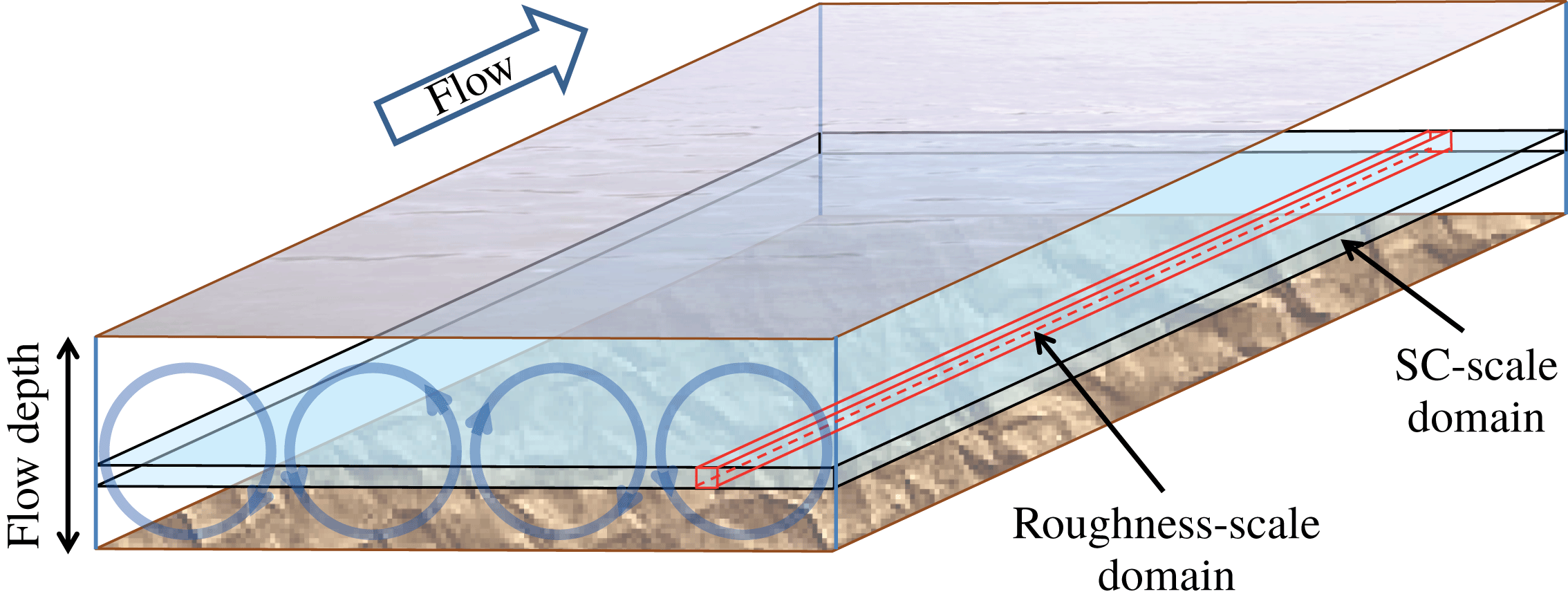
Roughness-scale and SC-scale averaging domains in a rough-bed open-channel flow. Circles indicate secondary currents cells.
2.3 Partitioning of the total dispersive stress
There may be situations when there is more than one source of mean flow heterogeneity. For example, the roughness effects on the flow may be superimposed with the effects of the secondary currents (SCs) which are typically scaled with the flow depth. Under secondary currents in straight channels we consider helical motions visible in time- and streamwise-averaged flow fields (e.g. Nezu & Nakagawa Reference Nezu and Nakagawa1993). In cross-sectional planes they are typically expressed with counter-rotating motions preserved along the flow. In this case, the total dispersive stresses are formed due to combined effects of bed roughness and SCs. Close to the bed the main contribution to the dispersive stresses is expected from the roughness effects which typically quickly die out away from the bed, where the SCs may become the dominant contributor (e.g. figures 6–8 to be discussed in § 4.1). Thus, in principle the total dispersive stress in uniform double-averaged flow over (statistically) homogeneous in streamwise direction rough bed can be subdivided into two terms: (i) a term responsible for the roughness-scale effects; and (ii) a term responsible for the secondary current effects. This subdivision is motivated by the observations that OCFs over rough beds (e.g. Nikora & Roy Reference Nikora, Roy, Church, Biron and Roy2012) are often filled with helical secondary currents which may serve as an additional source of dispersive stresses typically occurring at a larger scale compared to the roughness-generated dispersive stresses. The subdivision makes use of two different averaging domains: (i) a thin elongated domain with a streamwise dimension that well exceeds the roughness correlation length, while the spanwise dimension is much smaller than the flow depth
 $H$
(or in other words much smaller than the transverse size of the SC cells; subsequently called the ‘roughness-scale’ domain); and (ii) a thin spanwise-extended domain that is several flow depths wide and several roughness correlation lengths long (subsequently called the ‘SC’ domain). A sketch in figure 1 illustrates both domains. Use of the first domain allows roughness effects to be isolated while with the second domain both roughness and SC contributions to the total dispersive stress are accounted for. If we use the double-averaged equations based on the SC domain, then by additionally employing a ‘roughness-scale’ averaging we can distinguish contributions to the total dispersive stresses due to the bed roughness and secondary currents (see appendix A for details). This approach yields the following decomposition of the total dispersive stress
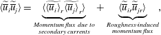
where
 $\widetilde{\overline{u}}_{i}=\overline{u}_{i}-\langle \overline{u}_{i}\rangle =\widetilde{\langle \overline{u}_{i}\rangle }_{r}+\widetilde{\overline{u}}_{ir}$
is a dispersive fluctuation based on the SC averaging domain;
 $\langle \overline{u}_{i}\rangle$
is the double-averaged velocity based on the SC averaging domain, defined by angular brackets
 $\langle \cdots \rangle$
with no subscript;
 $\widetilde{\overline{u}}_{ir}=\overline{u}_{i}-\langle \overline{u}_{i}\rangle _{r}$
is a dispersive component based on the ‘roughness-scale’ averaging domain;
 $\langle \overline{u}_{i}\rangle _{r}$
is the double-averaged velocity based on the ‘roughness-scale’ averaging domain, defined by angular brackets
 $\langle \cdots \rangle$
with subscript
 $r$
;
 $\widetilde{\langle \overline{u}_{i}\rangle }_{r}=\langle \overline{u}_{i}\rangle _{r}-\langle \overline{u}_{i}\rangle$
is a dispersive component due to the secondary currents alone. The final equation underpinning our estimates in §§ 4.2–4.4 can then be obtained from (2.3) and (2.10) as

It should be noted that the dispersive stress partitioning, proposed in this section, stems from the definition of the secondary currents in OCFs as helical motions visible in time- and streamwise-averaged flow fields (e.g. Nezu & Nakagawa Reference Nezu and Nakagawa1993). However, this conventional definition is not unique, as in principle there may be ‘meandering’ time-averaged SC cells, among other possible scenarios. After streamwise averaging of such meandering cells they may appear invisible in time- and streamwise-averaged flow fields, invalidating the proposed partitioning. Furthermore, the streamwise wavelengths of SC meandering may be comparable to the roughness scales, making the separation of roughness-induced and SC-induced contributions problematic, if possible at all. This later case is suggested by a recent paper of Chan et al. (Reference Chan, MacDonald, Chung, Hutchins and Ooi2018), who reported a comprehensive study of flow structure in pipes covering a wide range of three-dimensional roughnesses of the staggered type. The emergence of near-wall ‘meandering’ SCs, with scales comparable to the scales of roughness elements, is clearly seen in their figure 14 (Chan et al. Reference Chan, MacDonald, Chung, Hutchins and Ooi2018). That said, the SCs observed in our work, as will be shown in § 4.1, fit the conventional definition very well making the partitioning proposed here appropriate.
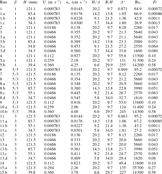
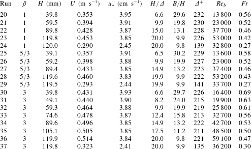
Flow and roughness characteristics for LES data set.
 $\unicode[STIX]{x1D6FD}$
is spectral slope,
 $H$
is mean flow depth,
 $U$
is cross-sectionally averaged mean velocity,
 $u_{\ast }$
is shear velocity computed using streamwise pressure gradient as explained in § 3.3,
 $H/\unicode[STIX]{x1D6E5}$
is relative submergence,
 $\unicode[STIX]{x1D6E5}=4\unicode[STIX]{x1D70E}_{z}$
,
 $B/H$
is aspect ratio,
 $B$
is flow width,
 $\unicode[STIX]{x1D6E5}^{+}=u_{\ast }\unicode[STIX]{x1D6E5}/\unicode[STIX]{x1D708}$
is roughness Reynolds number,
 $Re_{b}=UH/\unicode[STIX]{x1D708}$
is bulk Reynolds number,
 $Fr=U/(gH)^{0.5}$
is Froude number,
 $\unicode[STIX]{x1D708}$
is fluid kinematic viscosity and
 $g$
is acceleration due to gravity.
3 Laboratory experiments and large-eddy simulations
To apply the proposed decomposition (2.11), the authors have designed and completed extensive sets of laboratory experiments and complementary LES, covering a wide range of scenarios including a few overlap cases (tables 1–3). The overlap cases served to validate the accuracy of the LES by allowing direct comparisons of LES-predicted profiles of flow characteristics and friction factor contributions to those from the experiments. The same rough-bed geometries have been used in both laboratory experiments and LES, which produced velocity data sets with approximately the same spatial resolution. In the subsections below, the properties of the selected roughness types will be described first, followed by the outline of the key details of the laboratory experiments and LES.
Flow and roughness characteristics for PIV data set. Here
 $\unicode[STIX]{x1D6FD}$
is spectral slope,
 $H$
is mean flow depth,
 $U$
is cross-sectionally averaged mean velocity,
 $u_{\ast }=(gHS_{b})^{0.5}$
is shear velocity,
 $H/\unicode[STIX]{x1D6E5}$
is relative submergence,
 $\unicode[STIX]{x1D6E5}=4\unicode[STIX]{x1D70E}_{z}$
,
 $B/H$
is aspect ratio,
 $B$
is flow width,
 $\unicode[STIX]{x1D6E5}^{+}=u_{\ast }\unicode[STIX]{x1D6E5}/\unicode[STIX]{x1D708}$
is roughness Reynolds number,
 $Re_{b}=UH/\unicode[STIX]{x1D708}$
is bulk Reynolds number,
 $Fr=U/(gH)^{0.5}$
is Froude number,
 $\unicode[STIX]{x1D708}$
is fluid kinematic viscosity,
 $S_{b}$
is bed slope and
 $g$
is acceleration due to gravity.
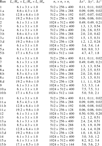
Parameters for LES runs. Here
 $L_{x}$
,
 $L_{y}$
and
 $L_{z}$
are the dimensions of the simulation domains,
 $H_{m}$
is maximum flow depth (i.e. distance between roughness troughs and water surface),
 $n_{x}$
,
 $n_{y}$
and
 $n_{z}$
are the total numbers of the simulation grid points,
 $\unicode[STIX]{x0394}x^{+}$
,
 $\unicode[STIX]{x0394}y^{+}$
and
 $\unicode[STIX]{x0394}z^{+}$
are the dimensionless grid sizes for the finest (near bed) grid resolution (normalised on viscous length
 $\unicode[STIX]{x1D708}/u_{\ast }$
).
3.1 Roughness characteristics
For our experiments and simulations we have selected single-valued self-affine fractal surfaces as they seem to represent a fairly general model of natural and man-made rough surfaces. Indeed, the studies of gravel-bed and sand-dune-bed rivers (e.g. Hino Reference Hino1968; Nikora, Sukhodolov & Rowinski Reference Nikora, Sukhodolov and Rowinski1997; Nikora, Goring & Biggs Reference Nikora, Goring and Biggs1998; Butler, Lane & Chandler Reference Butler, Lane and Chandler2001), the ocean floor (e.g. Bell Reference Bell1975), glaciated bedrocks and sub-glacial surfaces (e.g. Hubbard, Siegert & McCarroll Reference Hubbard, Siegert and McCarroll2000; Mankoff et al.
Reference Mankoff, Gulley, Tulaczyk, Covington, Liu, Chen, Benn and Głowacki2017), the surfaces of other planets (e.g. Turcotte Reference Turcotte1997; Nikora & Goring Reference Nikora and Goring2004) and a variety of machined surfaces (e.g. Majumdar & Tien Reference Majumdar and Tien1990) have demonstrated that all these surfaces can be described with one-dimensional power spectra (or second-order structure functions) of a similar shape. Typically, the observed spectra include three scale ranges with distinctly different behaviour: (i) a ‘saturation’ (white spectrum) range at low wavenumbers (
 $k_{x}<k_{xc1}$
); (ii) a scaling region at intermediate wavenumbers (
 $k_{xc1}<k_{x}<k_{xc2}$
) where the spectrum
 $S(k_{x})$
decays as a power function with a spectral exponent
 $\unicode[STIX]{x1D6FD}$
, i.e.
 $S(k_{x})\propto k_{x}^{-\unicode[STIX]{x1D6FD}}$
; and (iii) a ‘smooth’ region at high wavenumbers (
 $k_{x}>k_{xc2}$
) where the spectrum rapidly declines to zero (and thus within this region the surface is ‘smooth’, i.e. differentiable). Note that this schematisation assumes that the surface is a continuous single-valued field, which is a fair assumption even for granular surfaces if grain spacings are much smaller than the prevailing scales of surface fluctuations. The cutoff wavenumbers
 $k_{xc1}$
and
 $k_{xc2}$
define the upper and lower boundaries of the scaling region, respectively, with
 $(k_{xc1})^{-1}$
providing a measure of the roughness correlation length scale (which also depends on
 $\unicode[STIX]{x1D6FD}$
). The surface with such features may be classified as representative of self-affine fractal surfaces that exhibit, at least within a certain scale range, a power dependence of the amplitude
 $A$
of a disturbance on its wavelength
 $L$
, i.e.
 $A\propto L^{\unicode[STIX]{x1D6FC}}$
(e.g. Turcotte Reference Turcotte1997). The exponent
 $\unicode[STIX]{x1D6FC}$
, known as the Hurst (or Hölder) exponent, relates to the spectral exponent
 $\unicode[STIX]{x1D6FD}$
as
 $\unicode[STIX]{x1D6FD}=2\unicode[STIX]{x1D6FC}+1$
. The exponent
 $\unicode[STIX]{x1D6FC}$
can take a value between 0 and 1, with
 $\unicode[STIX]{x1D6FC}=1$
corresponding to the special case of self-similarity, thus yielding a range for
 $\unicode[STIX]{x1D6FD}$
from 1 to 3 for a surface to be classified as self-affine fractal (e.g. Turcotte Reference Turcotte1997). The described three-range spectral model is adopted in our work as most representative of naturally formed and man-made surfaces. It may be viewed as an extension of the approaches used in the studies of Anderson & Meneveau (Reference Anderson and Meneveau2011) and Barros, Schultz & Flack (Reference Barros, Schultz and Flack2015, Reference Barros, Schultz and Flack2018), where spectra of rough surfaces had a single range corresponding to our range (ii). For our study, we have chosen isotropic self-affine Gaussian surfaces with one-dimensional spectra as described above. Three self-affine fractal patterns, referred to hereafter as R1, R2 and R3, were generated using the inverse discrete Fourier transform of the designed spectra. Full details of the applied spectral synthesis procedure and the algorithms used are provided in Stewart et al. (Reference Stewart, Cameron, Nikora, Zampiron and Marusic2019).
For all three surface types, the wavenumbers defining the location and extent of the scaling range were the same, i.e.
 $k_{xc1}=0.02~\text{mm}^{-1}$
(i.e.
 $l_{x}=1/k_{xc1}=50~\text{mm}$
),
 $k_{xc2}=0.20~\text{mm}^{-1}$
(i.e.
 $l_{sm}=1/k_{xc2}=5~\text{mm}$
), as well as the surface standard deviation
 $\unicode[STIX]{x1D70E}_{z}=1.5~\text{mm}$
. The exponent
 $\unicode[STIX]{x1D6FD}$
in the scaling range (ii) is selected to be 1 for R1 (resembling ‘
 $-1$
’ scaling in near-bed velocity spectra),
 $5/3$
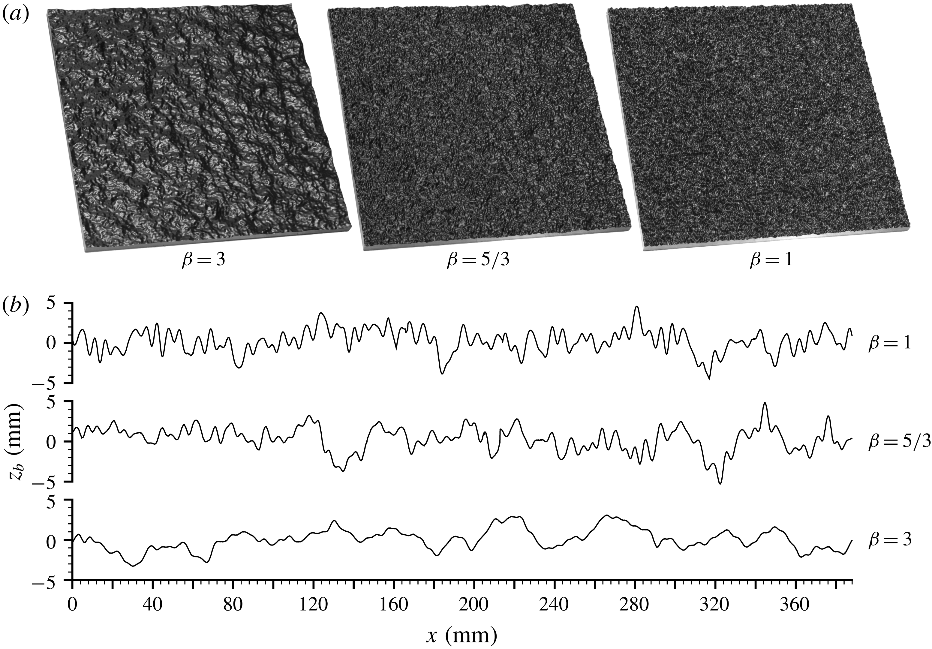
for R2 (resembling the inertial subrange exponent) and 3 for R3 (resembling scaling in sand-dune spectra). Although the selection of the exponents was rather intuitive, they do cover the whole range of possibilities. Figure 2 shows the resulting roughness patterns demonstrating the strong influence of the exponent
 $\unicode[STIX]{x1D6FD}$
while keeping scaling ranges and surface standard deviation the same for all three cases. The patterns are periodic in both
 $x$
and
 $y$
directions and thus can continuously cover the bed of our open-channel facility as well as to serve as a ‘numerical bed’ for LES runs (see §§ 3.2 and 3.3). The roughness height
 $\unicode[STIX]{x1D6E5}$
is defined as four standard deviations of the bed elevations to represent a 95.4 % range of their fluctuations, i.e.
 $\unicode[STIX]{x1D6E5}=4\unicode[STIX]{x1D70E}_{z}=6~\text{mm}$
. We do not employ directly the equivalent roughness height
 $k_{s}$
to characterise bed roughness in our study as its use requires the presence of the genuine logarithmic layer and validity of the logarithmic velocity distribution. Although our data do exhibit quasi-logarithmic velocity distribution above the roughness tops (see § 4.1), the relative submergence
 $H/\unicode[STIX]{x1D6E5}=5.7{-}20$
in our experiments is well below a suggested threshold value of 40 for the logarithmic layer to emerge (Jiménez Reference Jiménez2004). That said, it should be noted that the correlations obtained by Flack & Schultz (Reference Flack and Schultz2010) and Barros et al. (Reference Barros, Schultz and Flack2018) suggest that for the Gaussian rough surfaces the following approximate relation is valid:
 $k_{s}\approx (3.5{-}4.5)\unicode[STIX]{x1D70E}_{z}$
. Its equivalent presentation
 $k_{s}\approx (0.88{-}1.13)\unicode[STIX]{x1D6E5}$
provides additional support for choosing
 $\unicode[STIX]{x1D6E5}=4\unicode[STIX]{x1D70E}_{z}$
for characterising roughness heights in our study. Besides, Stewart et al. (Reference Stewart, Cameron, Nikora, Zampiron and Marusic2019) also showed that the spectral slope
 $\unicode[STIX]{x1D6FD}$
appears to be closely related to the roughness ‘effective slope’ ES, which is equal to the double solidity
 $\unicode[STIX]{x1D706}$
(i.e. the ratio of the projected frontal area of the roughness elements to the wall-parallel projected area; Napoli, Armenio & De Marchis Reference Napoli, Armenio and De Marchis2008; Flack & Schultz Reference Flack and Schultz2010). Estimates of solidity
 $\unicode[STIX]{x1D706}$
corresponding to
 $\unicode[STIX]{x1D6FD}=$
1, 5/3 and 3 were found to be
 $\unicode[STIX]{x1D706}=0.327$
, 0.219 and 0.102, respectively. The obtained data suggest an approximate relation
 $\unicode[STIX]{x1D706}=0.5ES=0.58\exp (-0.58\unicode[STIX]{x1D6FD})$
which, however, is not general and is limited to the roughness spectral shapes explored in our experiments.
Self-affine rough tiles used in the experiments and LES (a); (b) one-dimensional streamwise transects; the origin of the
 $z_{b}$
axis corresponds to the mean bed level. Tiles manufactured for laboratory experiments are shown.
For the laboratory experiments, the digital patterns have been used to manufacture the roughness tiles employing a three-step mould and cast procedure. First, a master plate was created for each of R1, R2 and R3 from acetal copolymer using a high-precision three-axis CNC milling machine. Second, moulds of each master plate were produced using a two-part addition cure room-temperature-vulcanizing (RTV) silicone rubber. Third, replicas of the master plates were then cast in the silicone moulds from epoxy resin. Owing to the large bed surface area of our laboratory facility it was necessary to manufacture at least 150 of these casts (‘tiles’) for each roughness pattern. As part of the final adjustments, the dimensions of the plates were reduced from the initial design value of 392 mm
 $\times$
392 mm to a final value of 388 mm
 $\times$
388 mm (
 $\pm$
0.1 mm). The prepared plates were aligned on the flume bed in a 50
 $\times$
3 array creating a continuous rough bed of repetitive patterns. The magnitude of potential discontinuities at the joints between the plates was appreciably less than
 $l_{sm}$
. A detailed assessment and analysis of the manufactured plates, as well as extensive measurements of the friction factor for a wide range of hydraulic conditions, are reported in Stewart et al. (Reference Stewart, Cameron, Nikora, Zampiron and Marusic2019). Specifically, Stewart et al. (Reference Stewart, Cameron, Nikora, Zampiron and Marusic2019) found that the exponent
 $\unicode[STIX]{x1D6FD}$
should be considered as a significant factor of the overall hydraulic resistance, in addition to the conventionally used length scales such as characteristic roughness heights and wavelengths. The results demonstrated that with all other parameters being the same, a decrease in
 $\unicode[STIX]{x1D6FD}$
leads to a visible increase in the friction factor. This effect was observed to be as great as 49 % between the R1 and R3 beds and it was not dependent on the channel aspect ratio. The present paper is, to a certain degree, a follow up of the work reported in Stewart et al. (Reference Stewart, Cameron, Nikora, Zampiron and Marusic2019), with a particular focus on the mechanisms contributing to the overall friction factor.
3.2 Laboratory experiments
Experiments were conducted in the Aberdeen Open Channel Facility (AOCF). The AOCF consists of an 18 m long and 1.18 m wide recirculating open-channel flume, an instrumental carriage that traverses the length of the flume with an integrated particle image velocimetry (PIV) system, along with data capture and analysis hardware and software systems. Flow is fed to the flume entrance tank by a pair of centrifugal pumps which are speed controlled in a closed loop system, with feedback provided by magnetic encoders attached to the pump drive shafts. The entrance tank has been optimised with honeycomb panels and guide vanes to ensure that the flow enters the channel uniformly distributed and free from large-scale turbulence and surface waves. The tail water level in the channel is controlled by adjusting a vertical slat weir at the channel exit to ensure flow uniformity. The flow depth distribution along the channel is calculated and adjusted before each experiment from profiles of the bed surface (using a laser triangulation sensor) and water surface (using a confocal displacement sensor). The relative standard errors of measured flow depth
 $H$
, bed slope
 $S_{b}$
and depth-averaged flow velocity
 $\widehat{U}$
(from PIV, see below) did not exceed 0.3 %, 1.4 % and 0.3 %, respectively, resulting in the maximum relative error in the friction factor of 1.5 %. This estimate gives the upper bound and corresponds to the overlap (with LES) validation cases that had smallest bed slope. The relative errors for all high Reynolds number cases are 5–8 times smaller.
Two configurations of the AOCF PIV system were used in this study: a streamwise orientated ‘mini’ mode for near-bed measurements, including the region below roughness tops and a transverse orientated ‘macro’ mode for measuring the flow region above the roughness tops. The ‘mini’ mode (figure 3
a) is a two-camera stereoscopic system with a measurement domain of
 $50~\text{mm}\times 25~\text{mm}$
(
 $x\times z$
). Three streamlined glass bottom boats sit at the water surface (one for each camera, and one for the laser sheet) to allow optical access to the flow. The camera boats contain water filled prisms to limit the distortion and internal reflection at the air–water interface. Flow disturbance from the boats is limited to a thin boundary layer (
 ${<}1.5$
mm thick) which does not interact with the measured region of the flow. We use Dalsa 4M180 cameras equipped with Nikon 60 mm lenses with aperture set to f/16, and capture data directly to a 24 TB solid state disk array. The light sheet was 0.7 mm thick and generated by an Oxford Lasers 532 nm Nd:YAG laser with pulse energy up to 100 mJ. The seeding particles for the ‘mini’ mode were neutrally buoyant 10–20 micron titania coated hollow glass microspheres, produced by Microsphere Technology Ltd.
‘Mini’-mode PIV configuration (a); ‘macro’-mode PIV configuration (b); footprint of the PIV measurement planes, with lines across the flow showing ‘macro’ mode and lines along the flow presenting ‘mini’-mode measurement planes, black-border squares show the roughness tiles (c); and transfer function
 $T$
of the ‘mini’ and ‘macro’ PIV measurement modes, with
 $\unicode[STIX]{x1D706}$
,
 $\unicode[STIX]{x1D706}_{x}$
,
 $\unicode[STIX]{x1D706}_{y}$
and
 $\unicode[STIX]{x1D706}_{z}$
denoting a generic wavelength and directional wavelengths in
 $x$
,
 $y$
and
 $z$
directions, respectively (d).
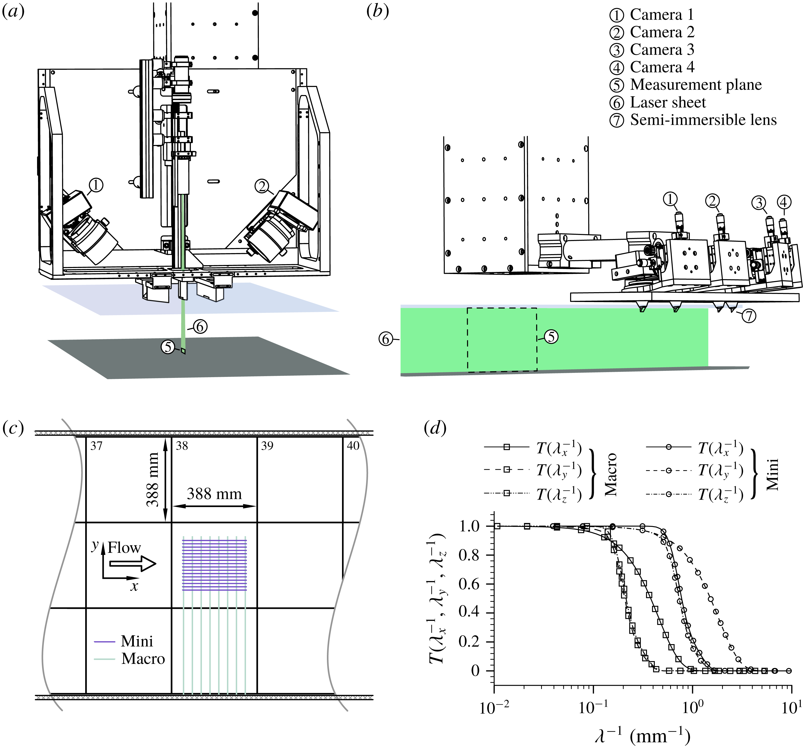
The ‘macro’ mode (figure 3
b) is a four-camera stereoscopic PIV system with a measurement domain of
 $225~\text{mm}\times 120~\text{mm}$
(
 $y\times z$
). For this mode we have designed and constructed semi-immersible camera lenses that penetrate approximately 10 mm through the water surface. The lenses have a 7 mm right angle prism mirror attached to the tip, which orientates the viewing direction of the downward facing cameras in the upstream direction. The cameras are placed 500 mm downstream of the transverse orientated light sheet so that the small wakes from the semi-immersed lenses cannot disturb the upstream measurement domain. The lenses have a fixed aperture of f/16. Larger silver coated seeding particles with diameters of 20–32 microns were used for the ‘macro’ mode. The light sheet was 2.8 mm thick and entered the flow through the glass side wall of the channel.
Both ‘mini’ and ‘macro’-mode PIV systems are attached to a robotic 3-axis platform that can programmatically position the respective measurement domains anywhere in the channel without manual adjustments or recalibration. Axis positions are recorded with sub-micron noise and resolution by linear-scale optical encoders attached to each axis. Calibrations of the stereoscopic PIV systems are performed by capturing images of a backlit 50 micron diameter pinhole from different camera positions. The experimental scenarios covered by PIV measurements are shown in table 2.
A series of 128 ‘mini’-mode and 32 ‘macro’-mode measurements were carried out for each flow scenario and roughness configuration to provide sufficient data for double averaging. The measurements were made 12 m (100–300 flow depths) from the flume entrance ensuring fully developed flow conditions. The ‘mini’-mode measurement planes were configured in an 8
 $\times$
16 (
 $x\times y$
) grid with a step size of
 $40~\text{mm}\times 15~\text{mm}$
. Each measurement plane was recorded for 100 s at a sampling rate of 10 Hz. The combined footprint of the 128 planes is shown in figure 3(c). The 32 ‘macro’ mode measurement planes were configured on a grid of 8
 $\times$
4 (
 $x\times y$
) with a grid step of
 $40~\text{mm}\times 165~\text{mm}$
(figure 3
c). Each of the ‘macro’ measurement planes were sampled for 240 s at a sampling rate of 10 Hz.
The PIV images were analysed using an iterative deformation method (IDM) PIV algorithm (Cameron Reference Cameron2011). For our analysis we have selected 64
 $\times$
64 pixel Blackman weighted interrogation regions with 52 pixel overlap between neighbouring interrogation regions, and a stretched sin-cardinal (sinc) kernel to low-pass filter the velocity field between each of the 8 iterations of the algorithm. The transfer functions that reflect the low-pass filtering of the velocity field from the combined effects of the interrogation region size and the light sheet thickness is illustrated in figure 3(d). The mini-mode data have been used to obtain the double-averaged quantities using the roughness-scale averaging domain (
 $0.7\times 0.7\times 388$
mm). The macro-mode data were employed to compute the SC-scale double-averaged quantities within the domain (
 $2.5~\text{mm}\times 388~\text{mm}\times 388~\text{mm}$
) at the channel centre (central tile in figure 3
c), including the depth-averaged velocity
 $\widehat{U}=H^{-1}\int _{z_{t}}^{z_{ws}}\unicode[STIX]{x1D719}\langle \overline{u}_{1}\rangle \,\text{d}z$
and ‘local’ friction factor
 $f=8\unicode[STIX]{x1D70F}_{0}/(\unicode[STIX]{x1D70C}\widehat{U}^{2})$
defined in §§ 1 and 2.1. The averaging times in the data analysis significantly exceeded turbulence length scales, typically being well above
 $70H/u_{\ast }$
. Similar domain sizes and averaging times have been used in LES data analysis, which is described below.
3.3 Large-eddy simulations
To carry out the LESs for selected scenarios (table 1), the in-house code Hydro3D was employed. The code has been previously validated and applied to study several flows of similar complexity (Bomminayuni & Stoesser Reference Bomminayuni and Stoesser2011; Kara, Stoesser & Sturm Reference Kara, Stoesser and Sturm2012; Bai, Fang & Stoesser Reference Bai, Fang and Stoesser2013; Kim, Stoesser & Kim Reference Kim, Stoesser and Kim2013; Kara et al. Reference Kara, Kara, Stoesser and Sturm2015b ,Reference Kara, Stoesser, Sturm and Mulahasan c ; Fraga et al. Reference Fraga, Stoesser, Lai and Socolofsky2016; McSherry et al. Reference McSherry, Chua, Stoesser and Mulahasan2018). Hydro3D is based on a finite-difference method employing a staggered Cartesian grid. The code solves the filtered Navier–Stokes equations for incompressible unsteady flow, i.e.
 $$\begin{eqnarray}\displaystyle & \displaystyle \frac{\unicode[STIX]{x2202}v_{i}}{\unicode[STIX]{x2202}x_{i}}=0 & \displaystyle\end{eqnarray}$$
 $$\begin{eqnarray}\displaystyle & \displaystyle \frac{\unicode[STIX]{x2202}v_{i}}{\unicode[STIX]{x2202}t}+\frac{\unicode[STIX]{x2202}v_{i}v_{j}}{\unicode[STIX]{x2202}x_{j}}=-\frac{1}{\unicode[STIX]{x1D70C}}\frac{\unicode[STIX]{x2202}{\dot{p}}}{\unicode[STIX]{x2202}x_{i}}+\frac{\unicode[STIX]{x2202}(2\unicode[STIX]{x1D708}\unicode[STIX]{x1D61A}_{ij})}{\unicode[STIX]{x2202}x_{j}}-\frac{\unicode[STIX]{x2202}\unicode[STIX]{x1D70F}_{ij}}{\unicode[STIX]{x2202}x_{j}}, & \displaystyle\end{eqnarray}$$
where
 $v_{i}$
is the resolved velocity in the
 $i$
th direction (
 $i=1$
, 2 and 3 correspond to
 $x$
-,
 $y$
- and
 $z$
-directions, respectively) and
 $x_{i}$
is the space coordinate vector;
 ${\dot{p}}$
is resolved pressure; and
 $\unicode[STIX]{x1D61A}_{ij}$
denotes the filtered strain-rate tensor
 $\unicode[STIX]{x1D61A}_{ij}=1/2(\unicode[STIX]{x2202}v_{i}/\unicode[STIX]{x2202}x_{j}+\unicode[STIX]{x2202}v_{j}/\unicode[STIX]{x2202}x_{i})$
. The subgrid-scale (SGS) stress
 $\unicode[STIX]{x1D70F}_{ij}$
is defined as
 $\unicode[STIX]{x1D70F}_{ij}=-2\unicode[STIX]{x1D708}_{t}\unicode[STIX]{x1D61A}_{ij}$
where
 $\unicode[STIX]{x1D708}_{t}$
is the eddy viscosity. In this study, the wall-adapting local eddy viscosity (WALE) proposed by Nicoud & Ducros (Reference Nicoud and Ducros1999) is used to calculate
 $\unicode[STIX]{x1D708}_{t}$
and to obtain the subgrid stress model.
In Hydro3D, the convection and diffusion terms in the Navier–Stokes equations are approximated by fourth-order accurate central differences. An explicit 3-step Runge–Kutta scheme is used to integrate the equations in time, providing second-order accuracy. A fractional step method is employed, i.e. within the time step the convection and diffusion terms are solved explicitly first in a predictor step that is then followed by a corrector step during which the pressure and divergence-free velocity fields are obtained through a Poisson equation. The latter is solved iteratively through a multi-grid procedure. Hydro3D features a local mesh refinement (LMR) method allowing a finer mesh in the vicinity of the rough beds. As a result of using the fine mesh near the bed, the SGS eddy viscosity is of the same order of magnitude as the molecular viscosity even for the high-Reynolds-number validation (overlap) cases 5.a, 10.a and 15.a (table 1). Details of the LMR method and its validation are reported in Cevheri, McSherry & Stoesser (Reference Cevheri, McSherry and Stoesser2016).
Twenty-six LES runs were carried out in total. Details of the computational set-ups are provided in table 3, where the first column presents the run number, with a, b, c and d identifying different flow submergences
 $H/\unicode[STIX]{x1D6E5}$
. The second column shows the relative dimensions of the computational domain (
 $L_{x}$
,
 $L_{y}$
,
 $L_{z}$
) in terms of the maximum flow depth
 $H_{m}$
for each simulation. In general, the simulation domain covered two roughness tiles in the streamwise direction and one roughness tile in the spanwise direction; for the deepest flows this results in a domain size of the order
 $2\unicode[STIX]{x03C0}H_{m}\times \unicode[STIX]{x03C0}H_{m}\times H_{m}$
, typically accepted as adequate for resolving the largest structures in the flow. The third column of table 3 provides the total number of grid points in the streamwise,
 $n_{x}$
, spanwise,
 $n_{y}$
, and wall-normal,
 $n_{z}$
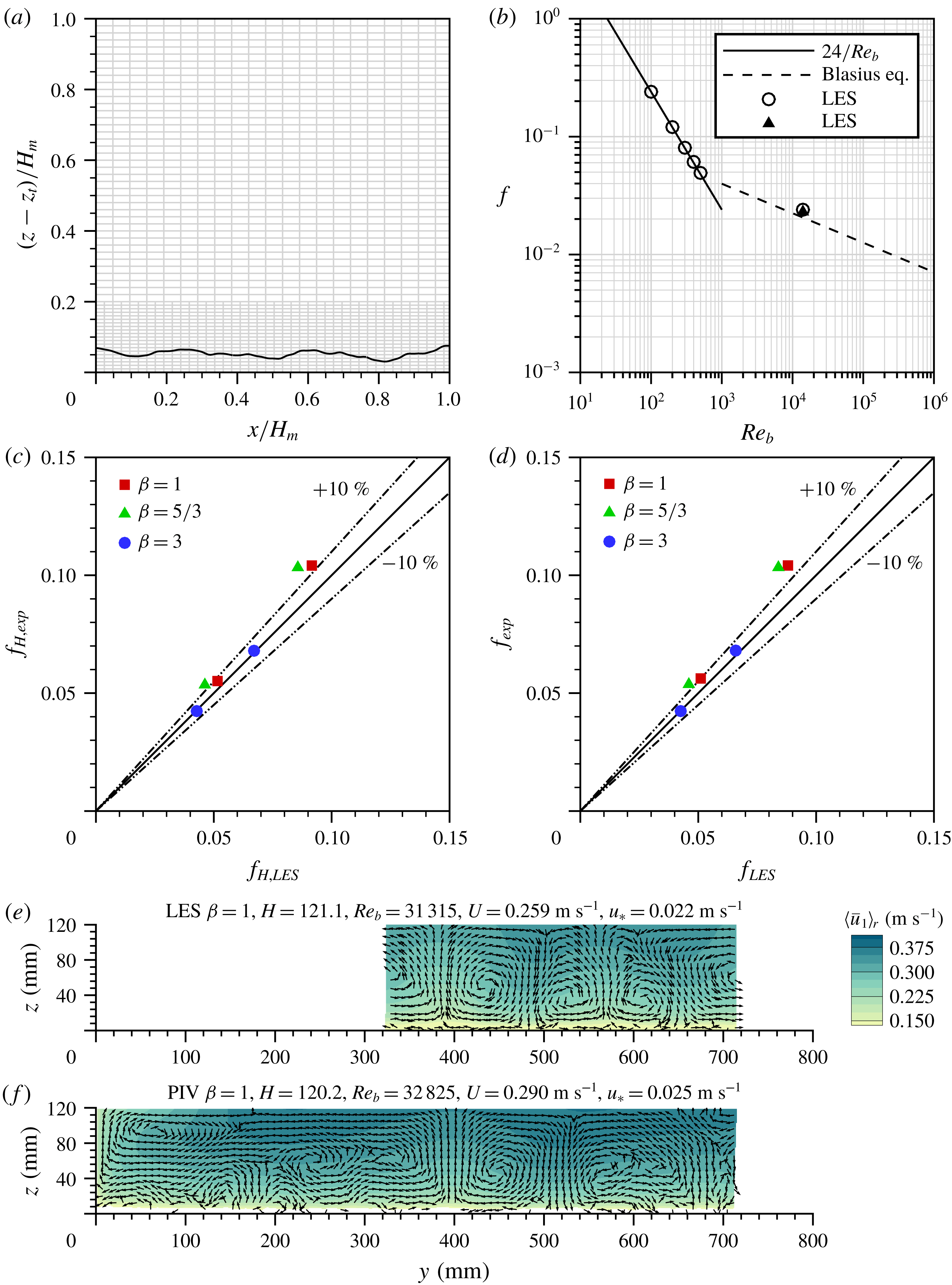
, directions, respectively. The domain is discretised with a locally refined mesh, a section of which is depicted in figure 4(a). The mesh consists of two parts: a coarser mesh (half of the resolution of the fine mesh, which makes it a 2:1 LMR) is employed in the upper region (80 % of the domain) whereas a finer grid is used in the near-wall region (20 % of the domain), to (i) allow the accurate representation of the roughness geometry and (ii) sufficiently resolve the flow features around individual roughness elements and hence their contributions to the drag. In the fourth column of table 3, the grid spacings in terms of wall units
 $\unicode[STIX]{x0394}x^{+}$
,
 $\unicode[STIX]{x0394}y^{+}$
,
 $\unicode[STIX]{x0394}z^{+}$
are listed for the finest grid resolution. The flow in the simulations is driven by a streamwise pressure gradient that is adjusted at every time step so that the constant bulk velocity is maintained. The LES-computed double- and depth-averaged pressure gradient
 $\text{d}\widehat{P}/\text{d}x$
is then used to calculate the domain-averaged wall shear stress and shear velocity, i.e.
 $\unicode[STIX]{x1D70F}_{0}=(\text{d}\widehat{P}/\text{d}x)H$
and
 $u_{\ast }=(\unicode[STIX]{x1D70F}_{0}/\unicode[STIX]{x1D70C})^{0.5}=[(1/\unicode[STIX]{x1D70C})(\text{d}\widehat{P}/\text{d}x)H]^{0.5}$
.
Part of the computational grid for
 $\unicode[STIX]{x1D6FD}=3$
(a); LES-predicted friction factors as a function of the bulk Reynolds number (symbols) and known analytical curves (lines) for laminar flows and smooth-bed turbulent flow (b); comparison of the friction factor estimates using experimental and LES data (see § 3.3 for details) (c,d); and comparison of velocity patterns from LES and PIV measurements; time- and streamwise-averaged data are shown (e,f). The coordinate
 $y=0$
corresponds to the right side wall of the flume.
In all LES runs, periodic boundary conditions are applied in the streamwise and spanwise directions, mimicking fully developed flow in both these directions. The water surface is treated as a frictionless rigid lid at which the free-slip condition is applied. The use of the rigid lid condition is deemed a reasonable treatment given the relatively low Froude number (table 1) and the experimentally observed fairly flat water surface. The no-slip condition is applied at the rough surfaces, employing a refined version (Kara, Stoesser & McSherry Reference Kara, Stoesser and McSherry2015a
; Ouro et al.
Reference Ouro, Harrold, Stoesser and Bromley2017; Ouro & Stoesser Reference Ouro and Stoesser2017) of the direct-forcing immersed-boundary method (IBM) first proposed by Uhlmann (Reference Uhlmann2005). The maximum grid spacing near the (rough) wall is
 $\unicode[STIX]{x0394}z^{+}/2$
being less than 5 wall units. Thus, the grid is fine enough for resolving, at least approximately, the viscous sublayer. The LES were run for at least 50 eddy turnover times (calculated as the ratio of water depth to the shear velocity) to collect the required statistics. In addition, the LES data were averaged spatially and convergence of the quantities was carefully monitored. All simulations are considered to be sufficiently converged.
In order to verify the code’s ability to predict the friction factor accurately, three series of runs for turbulent and laminar OCFs were carried out, i.e. (i) laminar flows; (ii) smooth-bed turbulent flow; and (iii) rough-bed turbulent flows. Figure 4(b) shows the LES-computed friction factors for laminar flows (open circles) as a function of the Reynolds number for five runs, together with the analytical solution
 $f=24/Re_{b}$
(solid line,
 $Re_{b}=UH/\unicode[STIX]{x1D708}$
; Graf & Altinakar Reference Graf and Altinakar1998). As can be seen in this figure, the simulations reproduce the friction factor change with increasing Reynolds number fairly accurately. A simulation of turbulent smooth-bed flow (
 $Re_{b}=10\,400$
) shows that the friction factor values, evaluated using
 $\text{d}\widehat{P}/\text{d}x$
(open circle) and from (2.7) (black triangle), are essentially the same. They both match very well the Blasius empirical equation
 $f=0.224Re_{b}^{-1/4}$
, which was initially proposed for smooth-wall turbulent pipe flows and later widely adopted for wide open-channel flows (e.g. Yen Reference Yen2002). The third validation data set includes LES runs 5a, 5b, 10a, 10b, 15a and 15b that resemble experimental runs 24, 20, 29, 25, 37 and 30, respectively (tables 1 and 2). Figure 4(c,d) compares the estimates of the friction factors computed from
 $f_{H}=8(gHS_{b})/\widehat{U}^{2}$
(figure 4
c) and from (2.8),
 $f$
, (figure 4
d). Figure 4(c,d) demonstrates that the LES-predicted friction factor estimates match the experimentally obtained values reasonably well, with the data points being within a 10 % envelope except for the two shallow flows. The LES data for deeper flows (smaller friction factor) tend to match the experimental data better. A possible reason for this is that the rigid lid assumption is more appropriate for deeper flows, where water surface deformations are sufficiently small, while their effect may not be negligible for shallow flows. Also, the spanwise flow boundaries for LES and in the experiments are different (‘infinitely wide channel’ in the LES and smooth side walls in the experiments). This difference may explain why the experimental values of
 $f$
are always slightly larger than the LES values. Figure 4(e,f) presents contours of the time- and streamwise-averaged velocity
 $\langle \overline{u}_{1}\rangle _{r}$
with velocity vectors in the transverse plane for LES (e) and PIV (f) data. The agreement between simulations and experiments is favourable, with both revealing cells of the secondary currents located at approximately the same spanwise positions. The discrepancies in the patterns are mainly due to the spanwise boundaries and their effect on the development of the secondary currents in terms of strength, position and size. Overall, from figure 4 it can be concluded that the LES are able to predict flows over rough beds with sufficient accuracy, allowing extension of the experimental scenarios towards smaller Reynolds numbers using LES.
4 Results
In this section we first outline the key background features of flow turbulence in the studied scenarios (§ 4.1), followed by the assessments of the parameters involved in the friction factor decomposition (§ 4.2) and the mechanism-based contributions to the overall bed friction (§§ 4.3 and 4.4). The main attention in this analysis is paid to the identification of the effects of the roughness geometry (i.e.
 $\unicode[STIX]{x1D6FD}$
), relative submergence
 $H/\unicode[STIX]{x1D6E5}$
, bulk Reynolds number
 $Re_{b}=UH/\unicode[STIX]{x1D708}$
and the roughness Reynolds number
 $\unicode[STIX]{x1D6E5}^{+}=u_{\ast }\unicode[STIX]{x1D6E5}/\unicode[STIX]{x1D708}$
, which relates to
 $Re_{b}$
as
 $\unicode[STIX]{x1D6E5}^{+}=(u_{\ast }/U)(\unicode[STIX]{x1D6E5}/H)Re_{b}$
. We use the bulk Reynolds number
 $Re_{b}$
(based on the cross-sectionally averaged velocity
 $U$
) following the convention of open-channel studies. The difference between
 $Re_{b}=UH/\unicode[STIX]{x1D708}$
and
 $Re=\widehat{U}H/\unicode[STIX]{x1D708}$
for laboratory experiments is negligible as in our experiments
 $U/\widehat{U}$
is between 0.97 and 1.0. In LES data, the ratio
 $U/\widehat{U}$
is identically 1.0 as cross-sectional averaging in this case is the same as depth averaging when using the SC averaging domain. Note also that in computing
 $\unicode[STIX]{x1D6E5}^{+}=u_{\ast }\unicode[STIX]{x1D6E5}/\unicode[STIX]{x1D708}$
and friction factor
 $f=8u_{\ast }^{2}/\widehat{U}^{2}$
we have used estimates of the shear velocity obtained as
 $u_{\ast }=(gHS_{b})^{0.5}$
for the laboratory data and
 $u_{\ast }=[(1/\unicode[STIX]{x1D70C})(\text{d}\widehat{P}/\text{d}x)H]^{0.5}$
for the LES data. However, when normalising turbulence properties in figures 6–8 we used estimates based on the total fluid stress at the roughness tops, which is more appropriate for scaling turbulence quantities in OCFs (e.g. Cameron, Nikora & Stewart Reference Cameron, Nikora and Stewart2017). The relative standard errors of the parameters discussed in this section typically do not exceed 1–2 %.
Distribution of time-averaged velocities across and along the flow at different streamwise positions, with a plot for time- and streamwise-averaged velocities shown at the bottom.

Flow characteristics for PIV experiments with
 $\unicode[STIX]{x1D6FD}=1$
: vertical distributions of the double-averaged streamwise velocity (a), primary Reynolds stress (b), roughness-induced dispersive stress (c), secondary-current-induced dispersive stress (d), cross-sectional distributions of time- and streamwise-averaged velocity components (e) and bed elevations
 $z_{b}(x,y)$
(f). The origin of the wall-normal coordinate
 $z$
is at the mean bed level; the origin of the spanwise coordinate
 $y$
is at the right side wall of the flume.

4.1 Background flow characteristics
A detailed analysis of the mean velocity fields and the turbulence structure in the studied flows is beyond the scope of this paper and will be reported elsewhere. Here we will only identify some features that are pertinent to the objectives of this paper. These relate to the vertical distributions of the double-averaged quantities based on the SC averaging domain (as described in § 2.3) that underpin the estimates of the terms in (2.11). In addition, the cross-sectional distributions of the mean velocity vectors and double-averaged velocities based on the roughness-scale averaging domain are also employed as they are helpful to understand the origin of the dispersive stresses due to the secondary currents. Before we outline the key features of the roughness-scale and SC-scale flow characteristics, it is useful to examine the evolution of the cross-sectional distributions of the time-averaged velocities at different locations along the flow. Figure 5 shows examples of such distributions revealing SC patterns that vary along the flow insignificantly, being nearly identical to the time- and streamwise-averaged pattern. These distributions are consistent with the conventional definition of secondary currents as helical motions identifiable in time- and streamwise-averaged flow fields, thus allowing the partitioning of the total dispersive stress as proposed in § 2.3.
Figure 6 summarises the PIV data for
 $\unicode[STIX]{x1D6FD}=1$
that can be viewed as generally representative of our combined PIV and LES data set. The upper four plots present vertical distributions of the double-averaged streamwise velocities
 $\langle \overline{u}_{1}\rangle$
, spatially averaged turbulent stresses
 $\langle \overline{u_{1}^{\prime }u_{3}^{\prime }}\rangle$
, roughness-induced dispersive stresses
 $\langle \widetilde{\overline{u}}_{1}\widetilde{\overline{u}}_{3}\rangle _{R}=\langle \widetilde{\overline{u}}_{1r}\widetilde{\overline{u}}_{3r}\rangle$
and dispersive stresses due to the secondary currents
 $\langle \widetilde{\overline{u}}_{1}\widetilde{\overline{u}}_{3}\rangle _{SC}=\langle \widetilde{\langle \overline{u}_{1}\rangle }_{r}\widetilde{\langle \overline{u}_{3}\rangle }_{r}\rangle$
, all normalised on the shear velocity
 $u_{\ast }$
(figure 6
a–d). The shifted vertical coordinate (
 $z-2\unicode[STIX]{x1D70E}_{z}$
) in this figure is normalised on the roughness height
 $\unicode[STIX]{x1D6E5}=4\unicode[STIX]{x1D70E}_{z}$
, where the origin of the
 $z$
coordinate is at the mean bed elevation.
The normalised velocity data for all studied submergences collapse on a single curve over the whole flow depth (figure 6
a), in agreement with fully rough conditions in PIV experiments. Below the roughness tops the velocity distribution is nearly linear with a quasi-logarithmic increase above the roughness tops, consistent with Nikora et al. (Reference Nikora, Koll, McEwan, McLean and Dittrich2004) and Yuan & Piomelli (Reference Yuan and Piomelli2014). The primary turbulent stress
 $\langle \overline{u_{1}^{\prime }u_{3}^{\prime }}\rangle$
changes linearly above the roughness tops, as one would anticipate for a two-dimensional double-averaged flow (e.g. Nikora et al.
Reference Nikora, McEwan, McLean, Coleman, Pokrajac and Walters2007). However, the close data collapse and linearity of
 $\langle \overline{u_{1}^{\prime }u_{3}^{\prime }}\rangle (z)$
below the roughness tops (figure 6
b) was not expected and needs further exploration. The same applies for the roughness-induced dispersive stress
 $\langle \widetilde{\overline{u}}_{1}\widetilde{\overline{u}}_{3}\rangle _{R}$
which attains a maximum around the roughness tops, (quasi)linearly reducing to zero upwards and downwards from this level (figure 6
c). The values of
 $\langle \widetilde{\overline{u}}_{1}\widetilde{\overline{u}}_{3}\rangle _{R}$
quickly approach zero just above the roughness tops. The dispersive stresses
 $\langle \widetilde{\overline{u}}_{1}\widetilde{\overline{u}}_{3}\rangle _{SC}$
due to the secondary currents are nearly zero within the roughness elements, growing upwards and reaching maximum values at mid-depth (figure 6
d). The relative magnitude of the dispersive stresses
 $\langle \widetilde{\overline{u}}_{1}\widetilde{\overline{u}}_{3}\rangle _{SC}/u_{\ast }^{2}$
systematically decreases with an increase in flow submergence
 $H/\unicode[STIX]{x1D6E5}$
. This behaviour is consistent with the velocity patterns in figure 6(e) depicting cross-sectional distributions of time- and streamwise-averaged velocity components in the transverse plane. In this figure one can observe that the flow contains secondary current cells that exhibit two key features: (i) the cells are best organised at the smallest submergence where they occupy the entire flow depth; with increase in submergence the cells deteriorate, particularly closer to the water surface; and (ii) the transverse positions of the cells do not change with the flow submergence, i.e. the transverse spacings between cells do not closely scale with the flow depth as often observed in previous studies of secondary currents in OCFs (e.g. Nezu & Nakagawa Reference Nezu and Nakagawa1993). These two features are quite unexpected, particularly the second feature that suggests the presence of some kind of streamwise ‘ridges’ on the bed that induce secondary currents (locking them to particular transverse locations). However, there are no obvious ‘ridges’ in the bed topography, which was designed to be random (figure 6
f). The only explanation of this ‘locking effect’ is that the observed secondary currents emerge in response to the repetitive effect of the selected roughness elements, as identical roughness tiles followed each other in the streamwise direction over the whole flume length (see § 3.1). A similar phenomenon was previously highlighted and discussed in Barros & Christensen (Reference Barros and Christensen2014), Anderson et al. (Reference Anderson, Barros, Christensen and Awasthi2015) and Vanderwel & Ganapathisubramani (Reference Vanderwel and Ganapathisubramani2015), who proposed a few mechanisms for the emergence of the secondary currents over random rough surfaces due to the repetitive effects of particular roughness elements. Among them are preferential flow pathways formed by repeating ‘valleys’ and ‘hills’ in the streamwise direction served as some kind of ‘interrupted’ streamwise ridges due to repeating roughness patterns employed in the experiments; effects of extreme wall shear stress at the tops of the highest roughness elements; persistent long wakes behind the largest roughness elements; and large spanwise gradients in bed surface topography. Our preliminary exploration of these and other possibilities did not provide yet a defensible explanation of our findings and it remains unclear exactly what mechanism is dominant or if a number of them are involved in some way. Nevertheless, a recent study of Chan et al. (Reference Chan, MacDonald, Chung, Hutchins and Ooi2018) lends strong support to the mechanism associated with preferential flow pathways enforced by repeating ‘hills’ and ‘valleys’ in the streamwise direction. Studying regular surface patterns with staggered roughness elements in pipe flows, Chan et al. (Reference Chan, MacDonald, Chung, Hutchins and Ooi2018) demonstrated the emergence of near-wall meandering time-averaged SCs, scaled with the wavelengths of the roughness elements (as visible in figure 14 in Chan et al.
Reference Chan, MacDonald, Chung, Hutchins and Ooi2018). Although in our case the roughness patterns were random at small scales (not regular staggered as in Chan et al.
Reference Chan, MacDonald, Chung, Hutchins and Ooi2018), at large scales they were regular due to the recurring tiles along the flow. This large-scale regularity could introduce preferential pathways of low- and high-momentum fluid, similar to those at the roughness scales investigated in Chan et al. (Reference Chan, MacDonald, Chung, Hutchins and Ooi2018). However, unlike Chan et al. (Reference Chan, MacDonald, Chung, Hutchins and Ooi2018), the spanwise spacing of influential ‘hills’ in our study appeared to be sufficiently large to prevent bed-induced meandering of SC cells (figure 5), thus permitting the partitioning of the dispersive stresses into roughness-induced and SC-induced contributions.
The aforementioned features of the
 $\unicode[STIX]{x1D6FD}=1$
case are representative of all three
 $\unicode[STIX]{x1D6FD}$
values for the LES data and for the
 $\unicode[STIX]{x1D6FD}=5/3$
PIV data (figure 7). However, the situation with PIV data for
 $\unicode[STIX]{x1D6FD}=3$
is different (figure 8), particularly in relation to the dispersive stresses due to the secondary currents. The maximum values of
 $\langle \widetilde{\overline{u}}_{1}\widetilde{\overline{u}}_{3}\rangle _{SC}/u_{\ast }^{2}$
initially decrease with an increase in the flow submergence (as in the cases of
 $\unicode[STIX]{x1D6FD}=1$
and
 $\unicode[STIX]{x1D6FD}=5/3$
) but then start to grow and attain elevated values at the intermediate submergences (figure 8
d). This effect is likely due to the cell amalgamation with increase in flow submergence (figure 8
e). As an example, considering two cells at
 $y\approx 475~\text{mm}$
and
 $y\approx 560~\text{mm}$
at
 $H=40~\text{mm}$
, one can observe their merging amid increasing depth, with a complete replacement by a larger cell at
 $H=75~\text{mm}$
. With a further increase in the flow depth the cell development is similar to that for
 $\unicode[STIX]{x1D6FD}=1$
and
 $\unicode[STIX]{x1D6FD}=5/3$
, i.e. the cell strength deteriorates. No amalgamation effect is noted in PIV data for
 $\unicode[STIX]{x1D6FD}=1$
and
 $\unicode[STIX]{x1D6FD}=5/3$
and in LES data for all three roughness patterns. The reasons for the absence of cell amalgamation for
 $\unicode[STIX]{x1D6FD}=3$
in the LES data are unclear and may relate to the effects of the bulk Reynolds number, periodic boundary conditions, size of the simulation domain or use of the rigid lid boundary conditions which suppresses the water surface dynamics. The secondary currents dynamics and topology, including the amalgamation phenomenon at
 $\unicode[STIX]{x1D6FD}=3$
and its mechanism, will be discussed in detail elsewhere. Here we report this feature for the sake of explaining some of the findings in § 4.4.
Flow characteristics for PIV experiments with
 $\unicode[STIX]{x1D6FD}=5/3$
: vertical distributions of the double-averaged streamwise velocity (a), primary Reynolds stress (b), roughness-induced dispersive stress (c), secondary-current-induced dispersive stress (d), cross-sectional distributions of time- and streamwise-averaged velocity components (e) and bed elevations
 $z_{b}(x,y)$
(f). The origin of the wall-normal coordinate
 $z$
is at the mean bed level; the origin of the spanwise coordinate
 $y$
is at the right side wall of the flume.

Flow characteristics for PIV experiments with
 $\unicode[STIX]{x1D6FD}=3$
: vertical distributions of the double-averaged streamwise velocity (a), primary Reynolds stress (b), roughness-induced dispersive stress (c), secondary-current-induced dispersive stress (d), cross-sectional distributions of time- and streamwise-averaged velocity components (e) and bed elevations
 $z_{b}(x,y)$
(f). The origin of the wall-normal coordinate
 $z$
is at the mean bed level; the origin of the spanwise coordinate
 $y$
is at the right side wall of the flume.

4.2 Length scales
 $L_{\unicode[STIX]{x1D719}}$
,
$L_{\unicode[STIX]{x1D70F}}$
and the roughness parameter
$N$


The depth-roughness scale
 $L_{\unicode[STIX]{x1D719}}=(3\int _{z_{t}}^{z_{ws}}(z_{ws}-z)^{2}(1-\unicode[STIX]{x1D719})\,\text{d}z)^{1/3}$
emerges in the derivation of the friction factor decomposition (2.3) and is fully defined by the roughness geometry function
 $\unicode[STIX]{x1D719}=V_{f}/V_{0}$
and the maximum flow depth
 $H_{m}=z_{ws}-z_{t}$
(hence the name ‘depth-roughness length scale’). For a single-valued random bed surface (as in our case), the function
 $\unicode[STIX]{x1D719}(z)$
is equivalent to the cumulative probability distribution of bed elevations (Nikora et al.
Reference Nikora, Goring, McEwan and Griffiths2001). Since all three self-affine patterns in our study conform to the Gaussian probability distribution with the same mean and variance of bed elevations, the ratio
 $L_{\unicode[STIX]{x1D719}}/H$
depends on
 $H/\unicode[STIX]{x1D6E5}$
only and is independent of
 $\unicode[STIX]{x1D6FD}$
,
 $Re$
and
 $\unicode[STIX]{x1D6E5}^{+}$
, i.e. it is expected to be similar for all investigated scenarios. Within the range
 $5.7<H/\unicode[STIX]{x1D6E5}<20.2$
, covered in our PIV experiments and LES simulations, the directly computed values of
 $L_{\unicode[STIX]{x1D719}}/H$
closely collapse on a single curve that can be approximated by a power function
 $L_{\unicode[STIX]{x1D719}}/H=1.538(H/\unicode[STIX]{x1D6E5})^{-0.343}$
. For
 $5.7<H/\unicode[STIX]{x1D6E5}<20.2$
, the parameter
 $L_{\unicode[STIX]{x1D719}}/H$
varies from 0.88 to 0.54.
The drag length scale
 $L_{\unicode[STIX]{x1D70F}}=(\int _{z_{t}}^{z_{c}}(z_{ws}-z)^{2}F_{D}\text{d}z/\int _{z_{t}}^{z_{c}}F_{D}\,\text{d}z)^{0.5}$
also emerges in the derivation of (2.3) and can be viewed as a square root of the second moment of drag force with a reference point at the water surface. Thus,
 $L_{\unicode[STIX]{x1D70F}}$
is restricted to the range from
 $H_{c}=z_{ws}-z_{c}$
to
 $H_{m}=z_{ws}-z_{t}$
and it defines the vertical position at which the ‘effective’ drag force acting on the rough bed applies (in terms of the second moment as follows from the expression for
 $L_{\unicode[STIX]{x1D70F}}$
above). The scale
 $L_{\unicode[STIX]{x1D70F}}$
may be related to the distance from the water surface to the location of the resultant drag force defined as
 $Z_{\unicode[STIX]{x1D70F}}=\int _{z_{t}}^{z_{c}}(z_{ws}-z)F_{D}\,\text{d}z/\int _{z_{t}}^{z_{c}}F_{D}\,\text{d}z$
(Thom Reference Thom1971). For our data,
 $L_{\unicode[STIX]{x1D70F}}$
is close to
 $Z_{\unicode[STIX]{x1D70F}}$
: the difference between them is typically less than 2 %, sharply reducing with increase in the Reynolds number to less than 1 %. It is interesting to examine the ratio
 $(L_{\unicode[STIX]{x1D70F}}-H)/\unicode[STIX]{x1D70E}_{z}$
that characterises the penetration of the flow momentum into the roughness substrate, as it presents the relative distance of the effective drag location above/below the mean bed level. In general, the ratio
 $(L_{\unicode[STIX]{x1D70F}}-H)/\unicode[STIX]{x1D70E}_{z}$
should depend on the roughness type (i.e.
 $\unicode[STIX]{x1D6FD}$
), bulk Reynolds number
 $Re_{b}=UH/\unicode[STIX]{x1D708}$
, roughness Reynolds number
 $\unicode[STIX]{x1D6E5}^{+}=u_{\ast }\unicode[STIX]{x1D6E5}/\unicode[STIX]{x1D708}$
and the relative submergence
 $H/\unicode[STIX]{x1D6E5}$
, i.e.
 $(L_{\unicode[STIX]{x1D70F}}-H)/\unicode[STIX]{x1D70E}_{z}=F(\unicode[STIX]{x1D6FD},Re_{b},\unicode[STIX]{x1D6E5}^{+},H/\unicode[STIX]{x1D6E5})$
. To explore
 $(L_{\unicode[STIX]{x1D70F}}-H)/\unicode[STIX]{x1D70E}_{z}=F(\unicode[STIX]{x1D6FD},Re_{b},\unicode[STIX]{x1D6E5}^{+},H/\unicode[STIX]{x1D6E5})$
with our data, we first consider the effects of
 $Re_{b}$
and
 $\unicode[STIX]{x1D6E5}^{+}$
at a fixed relative submergence, i.e. excluding this variable from consideration. Figure 9(a) shows how
 $(L_{\unicode[STIX]{x1D70F}}-H)/\unicode[STIX]{x1D70E}_{z}$
varies with the bulk Reynolds number
 $Re_{b}$
at a fixed relative submergence
 $H/\unicode[STIX]{x1D6E5}=20$
: with increase in
 $Re_{b}$
it grows from
 $(L_{\unicode[STIX]{x1D70F}}-H)/\unicode[STIX]{x1D70E}_{z}\approx -1.7$
for very small
 $Re_{b}$
, to
 $(L_{\unicode[STIX]{x1D70F}}-H)/\unicode[STIX]{x1D70E}_{z}\approx 0$
at
 $Re_{b}\approx 15\,000$
and then with further increase in
 $Re_{b}$
the ratio
 $(L_{\unicode[STIX]{x1D70F}}-H)/\unicode[STIX]{x1D70E}_{z}$
fluctuates around 0. The plot
 $(L_{\unicode[STIX]{x1D70F}}-H)/\unicode[STIX]{x1D70E}_{z}$
against
 $\unicode[STIX]{x1D6E5}^{+}$
in figure 9(b) is qualitatively similar, reflecting certain interdependence of
 $Re_{b}$
and
 $\unicode[STIX]{x1D6E5}^{+}$
. Specifically, the saturation in the growth of
 $(L_{\unicode[STIX]{x1D70F}}-H)/\unicode[STIX]{x1D70E}_{z}$
occurs at
 $\unicode[STIX]{x1D6E5}^{+}\approx 50$
where
 $(L_{\unicode[STIX]{x1D70F}}-H)/\unicode[STIX]{x1D70E}_{z}$
reaches approximately 0. These results highlight an important physical effect related to the location of the effective drag force (in terms of the second force moment). At small
 $Re_{b}$
and
 $\unicode[STIX]{x1D6E5}^{+}$
, this location is above the mean bed level by up to
 $(1.5{-}1.7)\unicode[STIX]{x1D70E}_{z}$
i.e. it is fairly close to the level of the roughness tops. With increase in
 $Re_{b}$
and
 $\unicode[STIX]{x1D6E5}^{+}$
, the location of the effective drag force shifts down reaching the level of the mean bed or even slightly below it, reflecting flow penetration into the roughness stratum with increase in
 $Re_{b}$
and
 $\unicode[STIX]{x1D6E5}^{+}$
. No strong effect of the scaling exponent
 $\unicode[STIX]{x1D6FD}$
at
 $H/\unicode[STIX]{x1D6E5}\approx 20$
can be noted in figure 9(a,b), as the data points related to different
 $\unicode[STIX]{x1D6FD}$
look fairly mixed.
Effects of the bulk Reynolds number (a), roughness Reynolds number (b) and relative submergence (c–f) on the relative drag scale.

Effects of the bulk Reynolds number (a), roughness Reynolds number (b) and relative submergence (c)–(f) on the roughness parameter
 $N$
.
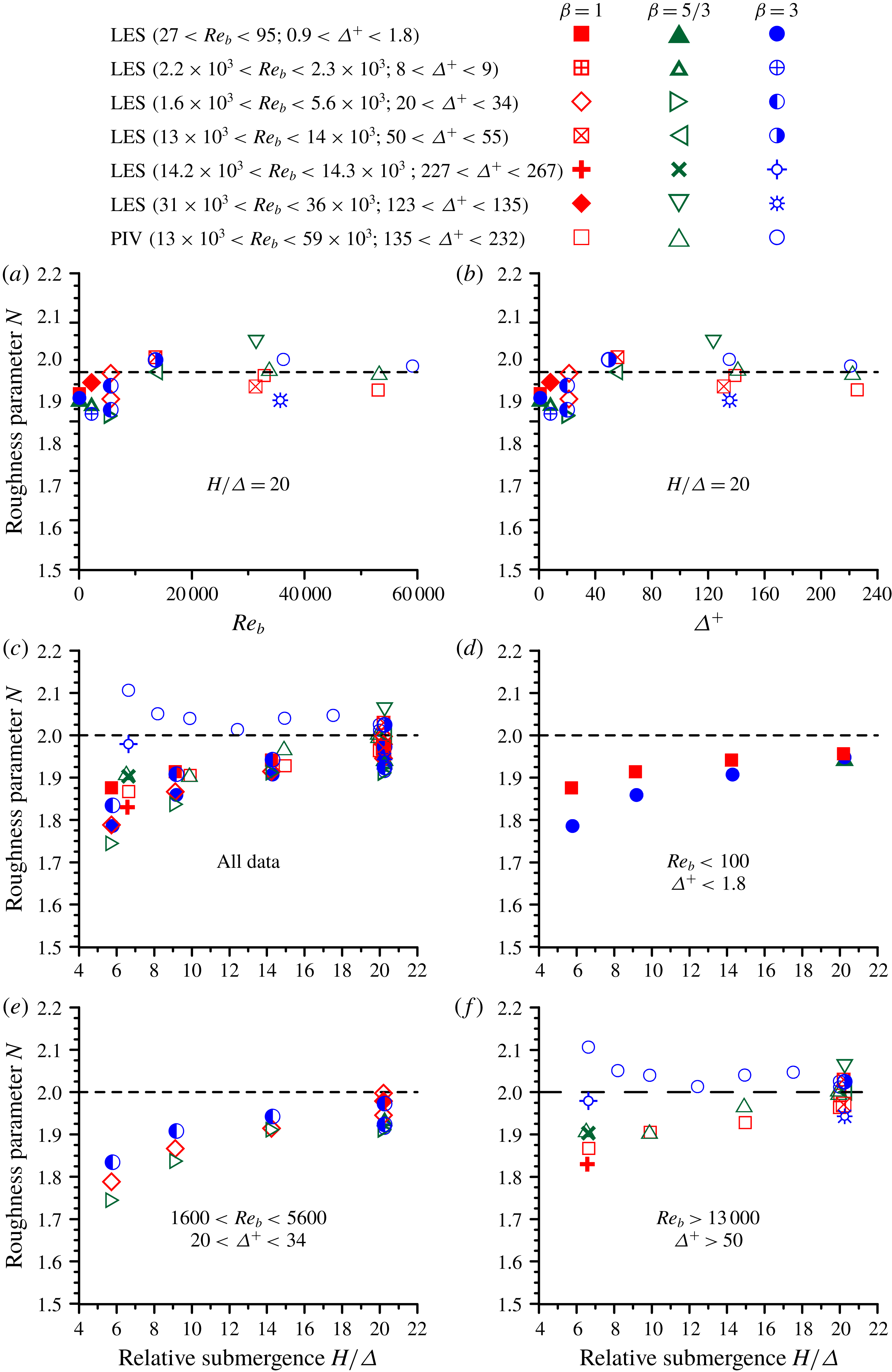
Figure 9(c–f) shows data on
 $(L_{\unicode[STIX]{x1D70F}}-H)/\unicode[STIX]{x1D70E}_{z}$
for the whole range of relative submergence
 $H/\unicode[STIX]{x1D6E5}$
in our study, with figure 9(c) presenting all data (all studied
 $Re_{b}$
) while figures 9(d)–9(f) show data subsets for three selected subranges of
 $Re_{b}$
: (i)
 $Re_{b}<100$
; (ii)
 $1600<Re_{b}<5600$
and (iii)
 $Re_{b}>13\,000$
. A general feature evident in all these plots is a fairly weak dependence of
 $(L_{\unicode[STIX]{x1D70F}}-H)/\unicode[STIX]{x1D70E}_{z}$
on the relative submergence
 $H/\unicode[STIX]{x1D6E5}$
. The effect of the Reynolds number noted above in figure 9(a,b) is also clearly seen in figures 9(d)–9(f). Another important feature that follows from the plots is the dependence of
 $(L_{\unicode[STIX]{x1D70F}}-H)/\unicode[STIX]{x1D70E}_{z}$
on the roughness geometry (i.e.
 $\unicode[STIX]{x1D6FD}$
), particularly noticeable at high Reynolds numbers in figure 9(f). Such dependence is not obvious at
 $H/\unicode[STIX]{x1D6E5}\approx 20$
in figure 9(a,b) but becomes apparent when considering a range of submergences. Figure 9(f) reveals a clear stratification of the data points with the highest values of
 $(L_{\unicode[STIX]{x1D70F}}-H)/\unicode[STIX]{x1D70E}_{z}$
for
 $\unicode[STIX]{x1D6FD}=3$
and the smallest values for
 $\unicode[STIX]{x1D6FD}=1$
. The decrease in the steepness of the roughness elements with increase in
 $\unicode[STIX]{x1D6FD}$
(Stewart et al.
Reference Stewart, Cameron, Nikora, Zampiron and Marusic2019) is reflected in the shift of the location of the effective drag force towards the roughness troughs (figure 9
f).
The effects of the relative scales
 $L_{\unicode[STIX]{x1D719}}/H$
,
 $L_{\unicode[STIX]{x1D70F}}/H$
and
 $H_{m}/H$
on the friction factor decomposition (2.3) are accounted for through a combined roughness parameter
 $N=3(L_{\unicode[STIX]{x1D70F}}/H)^{2}+(L_{\unicode[STIX]{x1D719}}/H)^{3}-(H_{m}/H)^{3}$
. In the limiting case of
 $H/\unicode[STIX]{x1D6E5}\rightarrow \infty$
, the parameter
 $N$
tends to 2.0 since
 $L_{\unicode[STIX]{x1D70F}}/H\rightarrow 1.0$
,
 $L_{\unicode[STIX]{x1D719}}/H\rightarrow 0$
and
 $H_{m}/H\rightarrow 1.0$
. The most influential among these scales is
 $L_{\unicode[STIX]{x1D70F}}/H$
as it enters the expression for
 $N$
with a factor of 3. The key tendencies for
 $N=F(\unicode[STIX]{x1D6FD},Re_{b},\unicode[STIX]{x1D6E5}^{+},H/\unicode[STIX]{x1D6E5})$
are illustrated in figure 10. Specifically, the following observations can be made: (i) at fixed
 $H/\unicode[STIX]{x1D6E5}\approx 20$
, the parameter
 $N$
increases with
 $Re_{b}$
from 1.86 until it reaches approximately 2.0 at
 $Re_{b}=15\,000$
, slightly fluctuating around this value afterwards (figure 10
a); (ii) similarly, at
 $H/\unicode[STIX]{x1D6E5}\approx 20$
it increases with
 $\unicode[STIX]{x1D6E5}^{+}$
approaching a saturation level of 2.0 at
 $\unicode[STIX]{x1D6E5}^{+}\approx 50$
(figure 10
b); (iii) the
 $Re_{b}$
and
 $\unicode[STIX]{x1D6E5}^{+}$
effects are also seen in the plots of
 $N$
versus
 $H/\unicode[STIX]{x1D6E5}$
that reveal a general tendency of
 $N$
towards 2.0 with increase in
 $H/\unicode[STIX]{x1D6E5}$
(figure 10
c–f); and (iv) there is a clear dependence of
 $N$
on the roughness geometry (i.e.
 $\unicode[STIX]{x1D6FD}$
), particularly at sufficiently high
 $Re_{b}$
and
 $\unicode[STIX]{x1D6E5}^{+}$
(figure 10
f). The obtained data show that the variation of the roughness parameter
 $N$
due to the effects of the bulk and roughness Reynolds numbers, relative submergence and exponent
 $\unicode[STIX]{x1D6FD}$
may not be negligible and can lead to errors of up to 5–6 % in the assessment of the friction factor, if not accounted for.
4.3 Reynolds number effects on the friction factor constituents
The effect of viscosity on the mechanism-based contributions
 $f_{i}$
to the overall friction factor
 $f$
can be assessed using PIV and LES data obtained at a fixed relative submergence
 $H/\unicode[STIX]{x1D6E5}\approx 20$
, to isolate potential effects of
 $H/\unicode[STIX]{x1D6E5}$
in the relation
 $f_{i}/f=F(\unicode[STIX]{x1D6FD},Re_{b},\unicode[STIX]{x1D6E5}^{+},H/\unicode[STIX]{x1D6E5})$
, where the subscript
 $i$
stands for viscous, turbulent and dispersive contributions defined in (2.11). Figure 11 illustrates the dependence on the bulk Reynolds number
 $Re_{b}$
of the relative contributions due to the viscous stress
 $f_{\unicode[STIX]{x1D708}}/f$
(figure 11
a), turbulent stress
 $f_{turb}/f$
(figure 11
b), roughness-induced dispersive stress
 $f_{d\text{-}R}/f$
(figure 11
c) and also the dispersive stress
 $f_{d\text{-}SC}/f$
induced by the secondary currents (figure 11
d). Taking into account an identity
 $\unicode[STIX]{x1D6E5}^{+}=(u_{\ast }/U)(\unicode[STIX]{x1D6E5}/H)Re_{b}$
one can expect some similarity between plots
 $f_{i}/f$
versus
 $Re_{b}$
and
 $f_{i}/f$
versus
 $\unicode[STIX]{x1D6E5}^{+}$
, as can be noted by comparing figures 11 and 12. The plots
 $f_{\unicode[STIX]{x1D708}}/f=F(Re_{b})$
and
 $f_{\unicode[STIX]{x1D708}}/f=F(\unicode[STIX]{x1D6E5}^{+})$
in these figures can be subdivided into two regions: (i) a region at low
 $Re_{b}$
and
 $\unicode[STIX]{x1D6E5}^{+}$
where
 $f_{\unicode[STIX]{x1D708}}/f\approx 1.0$
; and (ii) a region where the data closely collapse around curves
 $f_{\unicode[STIX]{x1D708}}/f\approx 1300Re_{b}^{-1.1}$
and
 $f_{\unicode[STIX]{x1D708}}/f\approx 2.5(\unicode[STIX]{x1D6E5}^{+})^{-1.0}$
at higher
 $Re_{b}$
and
 $\unicode[STIX]{x1D6E5}^{+}$
. The cross-over between these regions occurs at
 $Re_{b}=700$
and
 $\unicode[STIX]{x1D6E5}^{+}=2.5$
suggesting an emergence of additional momentum transfer mechanisms at higher
 $Re_{b}$
and
 $\unicode[STIX]{x1D6E5}^{+}$
. No data stratification due to the effects of
 $\unicode[STIX]{x1D6FD}$
can be observed in figures 11(a) and 12(a). The low-
 $Re_{b}$
region (i) corresponds to laminar flow. The scaling region (ii) likely reflects the role of the first term in (2.11). Indeed, the approximate relations
 $f_{\unicode[STIX]{x1D708}}/f\propto Re_{b}^{-1}$
and
 $f_{\unicode[STIX]{x1D708}}/f\propto (\unicode[STIX]{x1D6E5}^{+})^{-1.0}$
suggest that the dependence of the turbulent and dispersive stresses on the Reynolds number are much weaker compared to the viscous term, which is supported by figure 11(b–d).
Dependence of the mechanism-based contributions
 $f_{\unicode[STIX]{x1D708}}/f$
(a),
 $f_{turb}/f$
(b),
 $f_{d\text{-}R}/f$
(c) and
 $f_{d\text{-}SC}/f$
(d) to the overall friction factor
 $f$
on the bulk Reynolds number, at
 $H/\unicode[STIX]{x1D6E5}=20$
. The inclined dashed line shows a best fit approximation
 $f_{\unicode[STIX]{x1D708}}/f\approx 1300Re_{b}^{-1.1}$
.
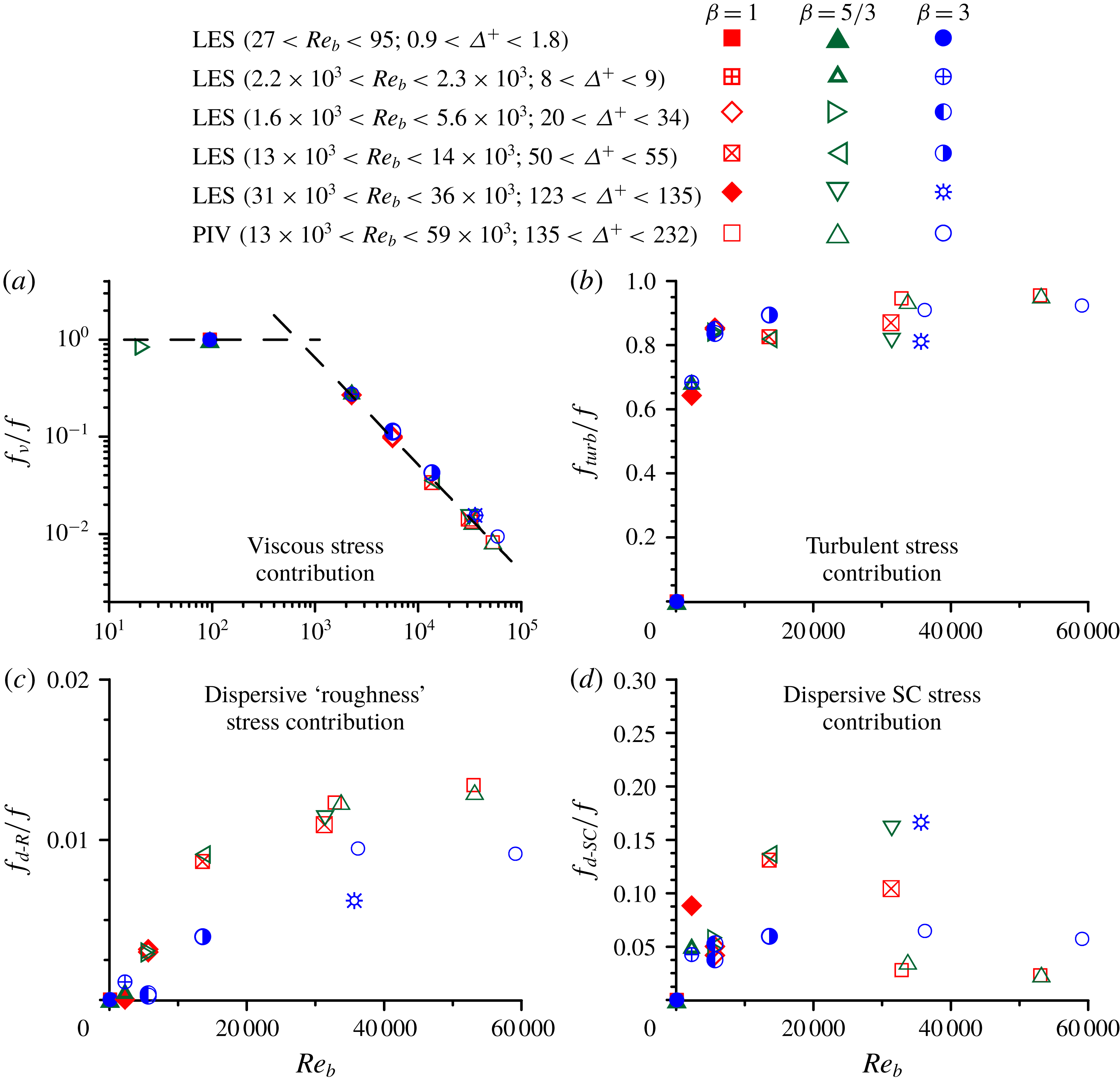
The contribution of the turbulent stress to the friction factor sharply increases from zero at low
 $Re_{b}$
and
 $\unicode[STIX]{x1D6E5}^{+}$
to 80 % at
 $Re_{b}\approx 4000$
and
 $\unicode[STIX]{x1D6E5}^{+}\approx 20$
and then continues to grow gradually (figures 11
b and 12
b). The bed geometry (i.e.
 $\unicode[STIX]{x1D6FD}$
) seems to have no influence on
 $f_{turb}/f$
at
 $H/\unicode[STIX]{x1D6E5}\approx 20$
, although it does have some influence at smaller submergences as will be shown in § 4.4. The plots
 $f_{d\text{-}R}/f$
versus
 $Re_{b}$
and
 $\unicode[STIX]{x1D6E5}^{+}$
in figures 11(c) and 12(c) reveal that the contribution of the roughness-induced dispersive stress at
 $H/\unicode[STIX]{x1D6E5}\approx 20$
is comparable to that from the viscous stress. There is a clear tendency of
 $f_{d\text{-}R}/f$
to rise with an increase in
 $Re_{b}$
and
 $\unicode[STIX]{x1D6E5}^{+}$
, with the growth rate being higher for
 $\unicode[STIX]{x1D6FD}=1$
and
 $\unicode[STIX]{x1D6FD}=5/3$
compared to
 $\unicode[STIX]{x1D6FD}=3$
. The effects of
 $Re_{b}$
and
 $\unicode[STIX]{x1D6E5}^{+}$
on the contribution
 $f_{d\text{-}SC}/f$
of the secondary currents to the friction factor are less clear: the data points are rather randomly mixed within a range
 $f_{d\text{-}SC}/f=3$
–20 % (figures 11
d and 12
d). This data spread reflects a variation in the strengths of the secondary currents observed in the LES outcomes as has been noted in § 4.1 and it might be inflated artificially due to boundary conditions or domain size. Nevertheless, it is clear that the contribution due to secondary currents is certainly not negligible and may well exceed those from the viscous stress and roughness-induced dispersive stress. In this regard it is useful to mention an interesting recent study of Modesti et al. (Reference Modesti, Pirozzoli, Orlandi and Grasso2018) who reported that the contribution of the secondary currents to the friction factor in a duct flow is of the order of 6 %, exactly within the range of our data for open-channel flows.
Dependence of the mechanism-based contributions
 $f_{\unicode[STIX]{x1D708}}/f$
(a),
 $f_{turb}/f$
(b),
 $f_{d\text{-}R}/f$
(c) and
 $f_{d\text{-}SC}/f$
(d) to the overall friction factor
 $f$
on the roughness Reynolds number, at
 $H/\unicode[STIX]{x1D6E5}=20$
. The inclined dashed line shows a best fit approximation
 $f_{\unicode[STIX]{x1D708}}/f\approx 2.5(\unicode[STIX]{x1D6E5}^{+})^{-1.0}$
.

4.4 Effect of relative submergence on the friction factor constituents
To evaluate the effect of
 $H/\unicode[STIX]{x1D6E5}$
on the variation of the relative contributions
 $f_{i}/f$
to the friction factor
 $f$
we consider data subsets at very low, intermediate and high Reynolds numbers. Starting with laminar flows (
 $Re_{b}<100$
), the LES data show that the viscous stress contribution
 $f_{\unicode[STIX]{x1D708}}/f$
is essentially 100 % while the contributions due to turbulent stress
 $f_{turb}/f$
and dispersive stress
 $f_{d\text{-}SC}/f$
due to the secondary currents are zero, as one would expect. The contribution of the roughness-induced dispersive stress
 $f_{d\text{-}R}/f$
is nearly zero too, varying from 0.04 % at low submergence to less than 0.01 % at
 $H/\unicode[STIX]{x1D6E5}\approx 20$
, (figure 13). The data points closely collapse around a single curve
 $f_{d\text{-}R}/f=0.013(H/\unicode[STIX]{x1D6E5})^{-2}$
, showing no clear effect of
 $\unicode[STIX]{x1D6FD}$
. The ‘
 $-2$
’ scaling and independence of
 $f_{d\text{-}R}/f$
on
 $\unicode[STIX]{x1D6FD}$
need further exploration and explanation. The data in figure 13 highlight possibilities for the emergence of an additional mechanism contributing to the overall drag in laminar flows, associated with the roughness-induced dispersive stress. This result is consistent with (2.9) and the regime of ‘rough-bed laminar flow’ proposed in § 2.2.
Dependence of the roughness-induced dispersive stress contribution
 $f_{d\text{-}R}/f$
on the relative submergence at low Reynolds number. The dashed line shows a best fit approximation
 $f_{d\text{-}R}/f=0.013(H/\unicode[STIX]{x1D6E5})^{-2}$
.

The data for the intermediate (LES) and high (PIV) Reynolds numbers are summarised in figure 14. The LES and PIV data points for
 $f_{\unicode[STIX]{x1D708}}/f$
,
 $f_{turb}/f$
,
 $f_{d\text{-}R}/f$
and
 $f_{d\text{-}SC}/f$
in this figure are well separated reflecting the Reynolds number effect already noted in § 4.3 for a fixed
 $H/\unicode[STIX]{x1D6E5}\approx 20$
. Another common feature in figures 14(a)–14(d) is the trend of increasing influence of the bed geometry with a decrease in the relative submergence
 $H/\unicode[STIX]{x1D6E5}$
: if at
 $H/\unicode[STIX]{x1D6E5}\approx 20$
the effect of
 $\unicode[STIX]{x1D6FD}$
is hard to note, it becomes more noticeable at smaller
 $H/\unicode[STIX]{x1D6E5}$
.
Dependence of the mechanism-based contributions
 $f_{\unicode[STIX]{x1D708}}/f$
(a),
 $f_{turb}/f$
(b),
 $f_{d\text{-}R}/f$
(c) and
 $f_{d\text{-}SC}/f$
(d) to the overall friction factor
 $f$
on the relative submergence at intermediate (LES) and high (PIV) Reynolds numbers.

The relative contribution
 $f_{\unicode[STIX]{x1D708}}/f$
of the viscous stress gradually reduces from
 ${\sim}$
20 % to
 ${\sim}$
10 % with increase in
 $H/\unicode[STIX]{x1D6E5}$
for intermediate
 $Re_{b}$
(LES data) and from
 ${\sim}$
2.5 % to
 ${\sim}$
1 % for high
 $Re_{b}$
(PIV data). The highest values of
 $f_{\unicode[STIX]{x1D708}}/f$
are observed for
 $\unicode[STIX]{x1D6FD}=3$
(figure 14
a). The overall trends in the variation of
 $f_{turb}/f$
are opposite to those of
 $f_{\unicode[STIX]{x1D708}}/f$
, also showing that the turbulent stress is the main contributor to the total bed friction (up to 96 % for
 $\unicode[STIX]{x1D6FD}=1$
and
 $\unicode[STIX]{x1D6FD}=5/3$
at
 $H/\unicode[STIX]{x1D6E5}\approx 20$
, figure 14
b). The relative contribution
 $f_{d\text{-}R}/f$
of the roughness-induced dispersive stress reaches up to 5–6 % for
 $\unicode[STIX]{x1D6FD}=5/3$
at the smallest submergence (figure 14
c), with all data subsets demonstrating a gradual decrease with increasing
 $H/\unicode[STIX]{x1D6E5}$
. Interestingly, the case of
 $\unicode[STIX]{x1D6FD}=3$
seems to be the least efficient in generating
 $f_{d\text{-}R}/f$
as the
 $\unicode[STIX]{x1D6FD}=3$
data serve as lower bounds for both intermediate and high Reynolds number data sets (figure 14
c).
The dispersive stress
 $f_{d\text{-}SC}/f$
due to the secondary currents complements
 $f_{d\text{-}R}/f$
to form the total dispersive stress, equation (2.10). At intermediate
 $Re_{b}$
(LES data), the relative contribution
 $f_{d\text{-}SC}/f$
of the secondary currents is within 1–6 %. The change of
 $f_{d\text{-}SC}/f$
with an increase in the relative submergence is monotonic for all three
 $\unicode[STIX]{x1D6FD}$
values, with a decreasing trend for
 $\unicode[STIX]{x1D6FD}=5/3$
and
 $\unicode[STIX]{x1D6FD}=3$
but with slightly increasing values for
 $\unicode[STIX]{x1D6FD}=1$
. The reason for this difference in trends between different values of
 $\unicode[STIX]{x1D6FD}$
is unclear. Additionally, there is a noticeable dependence of the
 $f_{d\text{-}SC}/f$
magnitude on
 $\unicode[STIX]{x1D6FD}$
: it generally increases with the change of
 $\unicode[STIX]{x1D6FD}$
from 1 to
 $5/3$
to 3 (figure 14
d), with the biggest differences at low
 $H/\unicode[STIX]{x1D6E5}$
which steadily reduce when
 $H/\unicode[STIX]{x1D6E5}$
increases to 20.
At high Reynolds numbers (PIV data), the relative contribution
 $f_{d\text{-}SC}/f$
also depends on
 $\unicode[STIX]{x1D6FD}$
in, qualitatively, the same way as for the case of intermediate
 $Re_{b}$
described above. The values of
 $f_{d\text{-}SC}/f$
steadily decrease with an increase in
 $H/\unicode[STIX]{x1D6E5}$
for
 $\unicode[STIX]{x1D6FD}=1$
and
 $\unicode[STIX]{x1D6FD}=5/3$
. However, the situation with the case of
 $\unicode[STIX]{x1D6FD}=3$
is quite different: there is a ‘hill’ in
 $f_{d\text{-}SC}/f$
within
 $H/\unicode[STIX]{x1D6E5}=10{-}18$
where the contribution of the secondary currents to the total friction factor exceeds 10 %, compared to 3–4 % for
 $\unicode[STIX]{x1D6FD}=1$
and
 $\unicode[STIX]{x1D6FD}=5/3$
. This ‘anomaly’ is most likely due to the effect of amalgamation of the secondary current cells observed for
 $\unicode[STIX]{x1D6FD}=3$
within this range of the relative submergence as noticed in § 4.1 and figure 8(e). The merger of smaller cells into larger cells produced a sharp increase in the dispersive stresses (figure 8
d) and, consequently, in the relative contribution of
 $f_{d\text{-}SC}/f$
(figure 14
d). At this point it is important to note that the relative increase of
 $f_{d\text{-}SC}/f$
within
 $H/\unicode[STIX]{x1D6E5}=10{-}18$
(figure 14
d) occurs with a simultaneous decrease in the relative turbulent stress contribution
 $f_{turb}/f$
(figure 14
b), suggesting the existence of some self-regulating interaction mechanism between SCs and turbulence. A similar effect has been earlier highlighted by Modesti et al. (Reference Modesti, Pirozzoli, Orlandi and Grasso2018) who reported that artificial suppression of SCs in their direct numerical simulations (DNS) of square duct flow led to a simultaneous increase in the turbulence contribution to the total friction factor, compensating for the lost effect of the secondary currents. These observations suggest that the suppression of one of the contributing mechanisms to the total friction factor may be compensated for by enhancement of the remaining mechanism(s).
5 Conclusions
This paper proposes a theoretically based relationship for the Darcy–Weisbach friction factor
 $f$
that opens new opportunities for exploring key contributing mechanisms for the case of rough-bed open-channel flows. It is shown that the friction factor can be split into at least five additive components, due to: (i) viscous stress; (ii) turbulent stress; (iii) dispersive stress (which in turn can be subdivided into two parts, due to bed roughness and secondary currents); (iv) flow unsteadiness and non-uniformity; and (v) spatial heterogeneity of fluid stresses in a bed-parallel plane. Compared to the previously proposed decompositions, our relationship explicitly accounts for the form drag and the effects of the dispersive stresses due to the bed roughness and secondary currents. These features make it possible to gain new insights into conventional roughness regimes of ‘flat-bed laminar flow’, ‘hydraulically fully smooth-bed turbulent flow’ and ‘hydraulically fully rough-bed turbulent flow’ as well as to propose new regimes of ‘rough-bed laminar flow’, ‘marginally rough-bed turbulent flow’, ‘mobile-rough-bed laminar flow’ and ‘mobile-marginally rough-bed turbulent flow’.
To explore the potential of the proposed relationship, we have assembled an extensive data set from laboratory experiments and LES for wide ranges of Reynolds number and relative submergence, related to flows over self-affine rough beds typical of natural and man-made surfaces. These data underpinned the exploration of the relative significance of mechanism-specific contributions to the friction factor and identification of the effects of roughness geometry, bulk Reynolds number, roughness Reynolds number and relative submergence. It is demonstrated that the dispersive stresses induced by bed roughness and secondary currents play a significant role in generating bed friction, although the turbulent stress contribution is leading. Importantly, our data suggest that there is an interdependence between the contributions of the turbulent and dispersive stresses (i.e. an increase in one may lead to a decrease in the other), consistent with a recent observation of Modesti et al. (Reference Modesti, Pirozzoli, Orlandi and Grasso2018). The contribution due to the viscous stress to the friction factor sharply reduces with an increase in the Reynolds number. The methodology proposed in this paper is conceptually fully transferrable to other flow types such as rough-wall boundary layers, pipes and conduits.
Acknowledgements
Financial support was provided by the EPSRC/UK project ‘Bed friction in rough-bed free-surface flows: a theoretical framework, roughness regimes, and quantification’ (grants EP/K041088/1 and EP/K04116/1). I.M. acknowledges the support of the Australian Research Council (grant FL120100017). The large-eddy simulations were carried out at Cardiff University’s high performance computer, which is part of the Supercomputing Wales project. Useful and stimulating discussions with M. Fletcher (Arup), P. Samuels (HR Wallingford), T. Schlicke (Scottish Environment Protection Agency) and J. Wicks (Jacobs) have been instrumental for this project and are gratefully acknowledged. The editor and three reviewers provided insightful comments and helpful suggestions that have been gratefully incorporated in the final version.
Appendix A. Partitioning of dispersive stresses into roughness-induced and SC-induced stresses
To separate contributions of bed roughness and secondary currents to the total dispersive stress in uniform double-averaged flow over a (statistically) homogeneous (in streamwise direction) rough bed we can consider two averaging domains: (i) ‘roughness-scale’ domain which is a thin elongated domain with a streamwise dimension that well exceeds the roughness correlation length while the spanwise dimension is much less than the transverse size of SCs; and (ii) ‘SC-scale’ domain which is a thin spanwise-extended domain several flow depths wide and several roughness correlation lengths long (figure 1). If we use double-averaged equations based on the SC-scale domain then by additionally employing a roughness-scale averaging we can distinguish contributions to the total dispersive stresses due to the bed roughness and due to the secondary currents. For this we employ the following decomposition of instantaneous hydrodynamic variables (using velocity
 $u_{i}$
as an example)

where
 $\bar{u}_{i}$
is local time-averaged velocity;
 $u_{i}^{\prime }=u_{i}-\bar{u}_{i}$
is turbulent velocity fluctuation;
 $\langle \overline{u}_{i}\rangle _{r}$
is double-averaged velocity based on the ‘roughness-scale’ averaging domain (spatial averaging based on the roughness-scale domain is defined by angular brackets
 $\langle \cdots \rangle _{r}$
with subscript
 $r$
);
 $\widetilde{\overline{u}}_{ir}=\overline{u}_{i}-\langle \overline{u}_{i}\rangle _{r}$
is dispersive component when using the ‘roughness-scale’ averaging domain;
 $\langle \overline{u}_{i}\rangle$
is double-averaged velocity when using the ‘SC-scale’ averaging domain (spatial averaging based on the ‘SC-scale’ domain is defined by angular brackets
 $\langle \cdots \rangle$
with no subscript);
 $\widetilde{\overline{u}}_{i}=\overline{u}_{i}-\langle \overline{u}_{i}\rangle =\widetilde{\langle \overline{u}_{i}\rangle }_{r}+\widetilde{\overline{u}}_{ir}$
is dispersive component based on the ‘SC-scale’ averaging domain; and
 $\widetilde{\langle \overline{u}_{i}\rangle }_{r}=\langle \overline{u}_{i}\rangle _{r}-\langle \overline{u}_{i}\rangle$
is dispersive component due to secondary currents. Using (A 1) we can obtain an expression for the total momentum flux as
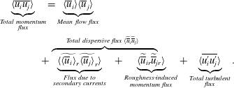
From (A 2) it follows that the total dispersive stress can be presented as a sum of the roughness-induced stress and SC-induced stress, i.e.
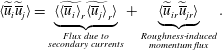


 Open access

