1. Introduction
Following the 2009 global recession, there have been changes in government spending and governance in several economies across the Middle East and Europe. Government spending as a percentage of gross domestic product ranged from 9 to 67 per cent across countries in 2002 but during the global recession in 2009 it changed, ranging from 11 to 52 per cent (World Bank, 2013). The composition of government spending also tends to change after recessions. For instance, European and Central Asian countries increased social assistance benefits as a response to the global recession (World Bank, 2013).Footnote 1 Also, periods of political change or turnover in governance tend to be associated with economic crises (Acemoglu and Robinson, Reference Acemoglu and Robinson2001, Reference Acemoglu and Robinson2006) and this may have been the case with the 2007 global financial crisis (Lloyd's, 2009).
There is literature linking the effect of changes in fiscal policy to pollution levels. A great deal of focus has been placed on the effect of government expenditure size on different pollutants (Bernauer and Koubi, Reference Bernauer and Koubi2012; Halkos and Paizanos, Reference Halkos and Paizanos2013). However, recent studies show that the composition of fiscal policies plays a crucial role in pollution reduction. López et al. (Reference López, Galinato and Islam2011) find that altering the composition of government spending from those that increase market failure to those that alleviate market failure reduces production-based air pollutants. López and Palacios (Reference López and Palacios2014) find that a similar alteration in the composition of government spending reduces pollution for the 12 richest European economies, while Islam and López (Reference Islam and López2015) find the same result for the USA.
The economic literature has typically focused on production-based pollutants, but some studies emphasize the importance of controlling consumption-based pollutants. McAusland (Reference McAusland2008) remarks that environmental issues such as air pollution, solid waste accumulation, climate change and ozone depletion are linked to the consumption of dirty goods. Residential waste accounts for about 55–65 per cent of solid waste. Chlorofluorocarbons, once found in home refrigeration units, are linked to accelerated depletion of stratospheric ozone.
There is also a growing body of literature linking changes in governance to pollution. One theory posits that democracy allows agents to truly reflect their environmental preferences as opposed to autocratic regimes (Farzin and Bond, Reference Farzin and Bond2006). Recent empirical estimates corroborate this finding (Bernauer and Koubi, Reference Bernauer and Koubi2009; Arvin and Lew, Reference Arvin and Lew2011). We have not come across a study that analyzes the role of fiscal policy changes within a political economy structure and its impact on pollution as a by-product during the consumption process.
This paper elucidates the mechanisms by which fiscal policies and democracy affect consumption pollutants. We develop a theoretical model that highlights the difficulty in controlling consumption pollutants via changes in the composition of government expenditure and the degree of democracy. We verify our theoretical results by estimating an empirical model. This is the only study to our knowledge that theoretically highlights the differences in the mechanisms by which fiscal policies and democracy affect consumption pollutants differently from production pollutants. Our results are important given that, during deep recessions, governments tend to alter the composition of spending. Our study shows how such changes in spending have diverse effects on environmental quality conditional on the political institutions.
We use a taxonomy proposed by López and Galinato (Reference López and Galinato2007) to distinguish two types of public expenditures by the government. López and Galinato (Reference López and Galinato2007) use the term ‘expenditures on public goods’ to mean any form of public spending that alleviates market failure. Spending that establishes institutions protecting the environment is an example of government expenditures that correct pollution externalities. Government spending that subsidizes education for low-income households is another example since it alleviates credit market constraints that prevent human capital accumulation. Also, government grants that provide health services to poor households or research and development grants have similar effects since they internalize positive externalities. Finally, it also includes public infrastructure spending that provides public goods.
López and Galinato (Reference López and Galinato2007) use the term ‘expenditures on private goods’ to represent expenditures to private firms that do not correct for any market failure and instead may even exacerbate market inefficiency. Examples include subsidies to fossil fuel production, agricultural subsidies and credit subsidies or tax breaks to specific firms. We use their terminology throughout the paper to delineate spending that alleviates market failure versus spending that does not.
The mechanisms relating fiscal spending to production pollutants differ from consumption pollutants. The reallocation of fiscal spending towards expenditures on public goods affects production pollution through a scale, composition and technique effect (López et al., Reference López, Galinato and Islam2011). A rise in the share of expenditures on public goods in total spending reduces production-based pollutants when there are larger output elasticities of expenditures on public goods in the non-polluting sector than the polluting sector and the marginal utility of consumption is elastic (López et al., Reference López, Galinato and Islam2011).
The mechanism that links consumption pollution and public spending is predicated on how government spending affects income and prices of goods faced by consumers. Public spending may affect future income of households. Credit-constrained households underinvest in education as a consequence of credit market imperfections (Grant, Reference Grant2007). Thus, subsidies to education and health can lead to more investment in education and higher future income (López et al., Reference López, Thomas and Wang2008). Public spending also allows the government to develop institutions that protect the environment by establishing and enforcing environmental regulations (Fullerton and Kim, Reference Fullerton and Kim2008).
The quality of governance also has an impact on the type of environmental regulations chosen by the government. Non-democratic regimes ruled by a select group may under-provide pollution reduction services because they face most of the environmental regulatory burden (Bernauer and Koubi, Reference Bernauer and Koubi2009). Democracy significantly reduces the level of corruption (Kolstad and Wiig, Reference Kolstad and Wiig2011). Any change in governance could affect prices via the choice of environmental regulations.
Our theory builds on Grossman and Helpman's (Reference Grossman and Helpman1994) seminal paper on the effect of lobbying on trade policies by extending it to evaluate environmental policies.Footnote 2 We incorporate different types of government spending and an environmental tax controlling a consumption pollutant. A representative household optimally selects its level of consumption and investment in human capital to earn income given the government's education subsidy. Pollution is created as a by-product during consumption. A competitive market exists for firms that produce the good and they all face a goods tax by the government. Firms influence the government's environmental tax choice through lobbying. The government selects the environmental tax level that maximizes a weighted welfare measure between aggregate economic welfare and lobby contributions.
Our theoretical model shows that government expenditures that alleviate market failure affect consumption pollution through two countervailing mechanisms: the income potential of consumers, which can increase consumption pollution, and the regulatory tax on firms, which can reduce consumption pollution. When the latter effect dominates the former effect, consumption pollution is reduced as expenditures on public goods rise. This result is more likely to happen when the government is more democratic. We also show that there are more conditions needed for expenditures on public goods to decrease consumption pollutants compared to production pollutants.
There is empirical support showing how higher government spending significantly affects human capital accumulation (Baldacci et al., Reference Baldacci, Clements, Gupta and Cui2008). When local government spending per capita increased in Brazil by 20 per cent over a four-year period, schooling and literacy both increased by 7 and 4 per cent, respectively (Litschig and Morrison, Reference Litschig and Morrison2013). Similarly, if government spending on public infrastructure rises, the marginal cost of education decreases, leading to an increase in schooling (Birdsall, Reference Birdsall1985; Behrman et al., Reference Behrman, Birdsall, Kaplan, Birdsall and Sabot1996).
There is also empirical support showing that more government spending raises compliance with environmental regulations. A field experiment in Norway's Environmental Protection Agency shows that an increase in audit frequencies increases compliance with environmental regulations (Telle, Reference Telle2013). Gray and Shimshack (Reference Gray and Shimshack2011) conclude that increased monitoring and enforcement of environmental policies leads to more compliance. Since a higher budget is required to increase monitoring activities, this literature shows that government spending leads to more stringently enforced environmental regulations.
We compile an unbalanced cross-country panel data set from 1986 to 1999 for 33 countries using carbon monoxide (CO) and nitrogen dioxide (NO2) as our consumption pollutants, along with measures of government spending and democracy. Our empirical estimates show that there is a positive and significant effect of lagged expenditures on public goods on income. The increase in income raises NO2 pollution but has no significant effect on CO. We also find a negative and significant direct effect, which reduces consumption pollution conditional on the government being democratic. The total effect of expenditures on public goods decreases consumption pollutants in democratic countries because the effect through regulations outweighs the effect through income. The opposite occurs when the government is autocratic. We also find that public spending composition alone does not significantly affect consumption pollutants. This may be because of more requirements needed for its reduction as suggested in our theory.
2. Theoretical model
The theoretical model accomplishes two objectives. First, we identify conditions needed for expenditures on public goods to decrease consumption pollutants and compare these conditions to those found by López et al. (Reference López, Galinato and Islam2011) which focused on production pollutants. Secondly, the theoretical model provides a baseline for estimating our empirical model.
There are m identical firms in a competitive market producing the consumption good, q c
 $$q^{c}=q\lpar x+k\comma \; g\rpar \comma \; $$
where k is capital input purchased by the firm, x is government expenditures on private goods that do not correct for market failure and g is government expenditures on public goods that correct for market failure.Footnote 3 Here, g can be thought of as research and development or public infrastructure that increases the productivity of output. We assume that technology is concave in all inputs, i.e. q k > 0, q kk < 0, q x > 0, q xx < 0, q g > 0, q gg < 0. Similar to López et al. (Reference López, Galinato and Islam2011), we assume x and k are perfect substitutes but k and g are complements, q gk > 0.Footnote 4
There are n identical consumers. The representative consumer's utility (U) depends on his or her consumption level net of disutility from the consumption pollution,
 $$U = u\lpar c \rpar - \theta Z\lpar nc\rpar \comma \; $$
where c is the consumption good, Z is pollution and θ is marginal disutility from pollution. Utility is concave in the consumption of the good. Pollution is increasing and convex in consumption.
Consumers earn income, f(h, g) which depends on the level of expenditures on public goods (g) and human capital, h. Educational investment and expenditures on public goods increase income at a decreasing rate. Here, g can be thought of as educational scholarships that relieve credit-constrained individuals. We also assume that expenditures on public goods positively affect marginal income such that f hg > 0. The budget constraint is
 $$f \lpar h\comma \; g \rpar = h + p\lpar Q\rpar c\comma \; $$
where price of investment in education is normalized to 1 and p(Q) is the equilibrium price in the competitive market. Price depends on aggregate consumption,
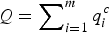 $Q=\sum\nolimits_{i=1}^{m} q_{i}^{c}$
, where
 $\displaystyle{{\partial p}\over{\partial Q}}\lt0$
.
To contrast the effects of government spending on consumption pollutants versus production pollutants, we adopt the assumptions used in López et al. (Reference López, Galinato and Islam2011) where they model the effect of government spending on production pollutants:
-
A1. Government spending that is directed towards expenditures on public goods benefits all sectors of the economy but the effects differ. The effect of expenditures on public goods is larger in the non-polluting sector than the polluting sector while expenditures on private goods directly target specific sectors of the economy and perfectly substitute for private capital investment.
-
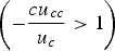
A2. Utility is strictly increasing and strictly concave in consumption (u c > 0 and u cc < 0) and the elasticity of marginal utility of consumption is greater than 1
 $\left(-\displaystyle{{cu_{cc}}\over {u_{c}}} \gt 1 \right)$
.
The first assumption is based on a stylized fact where government expenditures that subsidize production practices are usually targeted to the industrial sector but the expenditures on public goods may be much more dispersed (López et al., Reference López, Thomas and Wang2008). In our case, we do not have two production sectors. Instead we have a production sector and a household consumption sector. The production of the good does not create pollution so this would be a non-polluting sector, while the consumption of the good creates pollution so human capital investment which raises income is part of the polluting sector. The second assumption is based on empirical evidence showing that the elasticity estimates of marginal utility of consumption across countries are greater than 1.Footnote 5
The model defines a three-stage complete information game between the government and the lobby group of firms. The timing of the stages is as follows:Footnote 6
-
Stage 1. The lobby group offers a bribe schedule to the government to maximize industry profits.
-
Stage 2. The government sets its optimal environmental regulation level given the lobby group's strategy by maximizing a weighted sum of aggregate welfare and bribes.
-
Stage 3. Given the environmental regulation level, owners of firms choose how much to produce while consumers choose their consumption and human capital investment levels.
We solve the third stage and continue recursively.
2.1. Third stage: production of the good generating the consumption pollution
The firm maximizes profit by purchasing k from the world market,
 $$\Pi \lpar t\comma \; x\comma \; g\rpar = \max_k {\lpar p \lpar Q \rpar - t \rpar q \lpar x + k\comma \; g\rpar - rk}\comma \; $$
where r is an exogenously determined rate of capital and t is an environmental tax. The environmental tax creates a wedge between the producer price and consumer price. So, even if the tax is levied on firms creating a lower producer price, it will also affect consumers by raising the consumer price of the good as we show below.
The optimal condition that solves (4) is given by:
 $$\lpar p\lpar Q \rpar -t \rpar q_{k}=r\comma \; $$
which states that the value of the marginal product of capital is equal to the rental price. Given concavity of the production function, differentiation of (5) yields
 $\displaystyle{{dk}\over{dt}}\lt0$
where an increase in the tax reduces the amount of capital purchased. Since all firms are identical, all firms produce the same amount in equilibrium such that Q* = mq*, which implies that increasing tax reduces aggregate consumption because
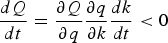 $\displaystyle{{dQ} \over {dt}} = \displaystyle{{\partial Q}\over{\partial q}} \displaystyle{{\partial q}\over{\partial k}} \displaystyle{{dk}\over{dt}}\lt0$
and raises price since
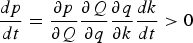 $\displaystyle{{dp}\over{dt}} = \displaystyle{{\partial p}\over{\partial Q}} \displaystyle{{\partial Q}\over{\partial q}} \displaystyle{{\partial q}\over{\partial k}} \displaystyle{{dk}\over{dt}}\gt0$
. A tax on the firm yields the same desired outcome to reduce consumption as a tax on consumers since the tax burden will be distributed between producers and consumers. Also, because g complements while x substitutes for firm production, we find
 $\displaystyle{{dk}\over{dx}}\lt0$
and
 $\displaystyle{{dk}\over{dg}}\gt0$
.
2.2. Third stage: consumers' behavior
Since we assume that consumers do not internalize their contribution to pollution when they make their optimal consumption decision, consumers maximize u(c) subject to (3) by selecting c and h. By substituting for c using (3) into u(c), we find the following condition,
 $$u_{c}\left(\displaystyle{{f_{h}-1}\over{p\lpar Q \rpar }}\right)=0. $$
Thus, the optimal level of educational investment satisfies the condition f h (h, g) = 1 where the marginal earnings equals the normalized price of education investment. The optimal h* is dependent on the government expenditures on public goods, i.e. h* = h*(g) The optimal consumption level is derived by substituting h* in (3) and solving c*.Footnote 7 Finally, we define consumer surplus as s(t, g)=u(c*)−p(Q)c*. The following lemma summarizes the effects of g and t on consumption, human capital investment and consumer surplus.
Lemma l:
Assuming that h and g are complements and
 $\displaystyle{{u_{c}^{\ast}}\over{p\lpar Q\rpar }}\gt1$
, we find
 $\displaystyle{{dh}\over{dg}}\gt0$
,
 $\displaystyle{{dc}\over{dg}}\gt0$
and
 $\displaystyle{{ds}\over{dg}}\gt0$
. Furthermore,
 $\displaystyle{{dh}\over{dt}}=0$
,
 $\displaystyle{{dc}\over{dt}}\lt0$
and
 $\displaystyle{{ds}\over{dt}}\lt0$
.
Proof See appendix A in the online appendix available at https://doi.org/10.1017/S1355770X17000237.□
The individual increases allocation to educational investment as expenditures on public goods rise. The rise in education investment leads to more earnings and higher consumption which, in turn, increase consumer surplus. Furthermore, there is no impact of taxes on h.Footnote 8 However, when the tax rises, less of the consumption good is purchased, which reduces consumer surplus.
2.3. Second stage: government's decision
Aggregate economic welfare, V, is composed of profit of all firms, consumer surplus, tax revenues and disutility from pollution, V=mΠ+ns(t, g)+T(t)−θZ, where T is the aggregate tax collected from firms T(t)=mtq. The government's welfare function is maximized by choosing environmental regulations that maximize a weighted sum of bribes and aggregate welfare similar to Grossman and Helpman (Reference Grossman and Helpman1994),
 $${\max_t G = \alpha V + B}\comma \; $$
where α is a measure of democratic participation or political competition similar in interpretation to that in Fredriksson et al. (Reference Fredriksson, Neumayer, Damania and Gates2005) and B is the bribe offered by the association on behalf of all firms. A large α implies that the government puts more weight on the welfare of the populace, which would mean allowing more inclusiveness and transparency in the decision-making process.
The first-order condition that solves the government's problem is
 $$\alpha \lpar t-\theta \rpar \displaystyle{{dQ}\over{dt}}+\alpha n\displaystyle{{ds}\over{dt}}+\displaystyle{{dB}\over{dt}}=0. $$
The first term represents the marginal benefit of raising the environmental tax, which is the reduced damages from pollution due to a reduction in equilibrium consumption. The last two terms show the marginal cost of increasing the tax in the form of a reduction in consumer surplus and a reduction in bribes received by the government.
2.4. First stage: lobby group's behavior
Firms funnel all contributions to an association that maximizes industry profit by optimally offering a bribe schedule to the government to influence its tax choice such that
 $${\max_{B} m\Pi - B}. $$
Taking the first-order condition with respect to B and re-arranging yields
 $$-Q = \displaystyle{{dB}\over{dt}}. $$
Bribes are paid by the association up to the point where the marginal cost of the bribe is equal to its marginal benefit. Bernheim and Whinston (Reference Bernheim and Whinston1986) and Grossman and Helpman (Reference Grossman and Helpman1994) refer to the above condition as the local truthfulness condition which ensures that the association will provide the government with a level of support. For an interior solution, it must be that
 $\displaystyle{{dB}\over{dt}}\lt0$
where the government will only receive more money from the association if tax regulations are lower.
From (8) and (10), the condition governing the tax regulation by the government is
 $$\alpha \lpar t-\theta \rpar \displaystyle{{dQ}\over{dt}}+\alpha n\displaystyle{{ds}\over{dt}}-Q=0. $$
For an interior solution, the marginal benefits of increasing the tax in the form of reduced pollution (the first term) has to be positive. Since
 $\displaystyle{{dQ}\over{dt}}\lt0$
and
 $\displaystyle{{ds}\over{dt}}\lt0$
from Lemma 1, for the first term to be positive it must be the case that t < θ. Without lobbying, the government maximizes V, leading to a Pigouvian tax rate of t = θ, thus allowing firms to bribe leads to a lower environmental tax.
The type of expenditure also has an effect on the level of regulations set by the government. Total differentiation of (11) yields the lemma below.
Lemma 2:
If k and x are perfect substitutes, then
 $\displaystyle{{dt}\over{dx}}\lt0$
. Also, if the marginal utility of consumption is elastic, i.e.,
 $-\displaystyle{{cu_{cc}}\over{u_{c}}}\gt1$
, and k and g have limited substitutability such that the elasticity of substitution, φ
k, g
, is bounded by
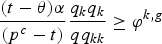 $\displaystyle{{\lpar t-\theta \rpar \alpha }\over{\lpar p^{c}-t \rpar }}\displaystyle{{q_{k}q_{k}}\over{qq_{kk}}}\ge \varphi^{k\comma g}$
, then
 $\displaystyle{{dt}\over{dg}}\gt0$
. Furthermore, given Lemma 1, we find
 $\displaystyle{{dc}\over{dt}}\displaystyle{{dt}\over{dg}}\lt0$
.
Proof: See online appendix A. □
An increase in x perfectly substitutes for a firm's capital purchase. This leaves more profit for the firm and more bribes to influence the government in lowering environmental regulations. On the other hand, an increase in g complements k purchased in the market. If the two inputs have limited substitutability, there may be fewer bribes offered by firms to influence the government leading to higher tax levels when g rises.
2.5. Subgame perfect Nash equilibrium
The following proposition summarizes the subgame perfect Nash equilibrium of the game.
Proposition 1: The subgame perfect Nash equilibrium occurs when:
2.6. The effect of expenditures and democracy on pollution
The total effect of g on consumption pollutants is calculated by taking the derivative of g with respect to Z where we find:
 $$\displaystyle{{dZ}\over{dg}}=n\left(\displaystyle{{dc}\over{df}}\displaystyle{{df}\over{dg}}+\displaystyle{{dc}\over{dt}}\displaystyle{{dt}\over{dg}}\right). $$
Here, g influences consumption pollution through two channels: income and environmental taxes. Based on Lemmas 1 and 2, the effect of g through the two channels has countervailing effects: an increase in g leads to higher income and increases pollution, whereas the impact through environmental taxes is to reduce pollution. We can further analyze the effect of expenditures on public goods on consumption goods by taking the total derivative of c* with respect to g. We summarize the conditions influencing such a relationship in the proposition below.
Proposition 2:
An increase in government expenditures on public goods entirely financed by an equal reduction in expenditures on private goods reduces consumption pollution if, and only if,
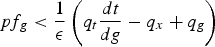 $pf_{g}\lt \displaystyle{{1}\over{\epsilon}}\left(q_{t}\displaystyle{{dt}\over{dg}}-q_{x}+q_{g} \right)$
where
 $\epsilon \equiv \displaystyle{{dQ}\over{dp}}\displaystyle{{p}\over{Q}}$
is the price elasticity of demand.
Proof: See online appendix A. □
An increase in expenditures on public goods is more likely to reduce consumption pollution under the following conditions: (C1) the marginal income from a change in expenditures on public goods (f
g
) is low; (C2) the marginal product of expenditures on public goods (q
g
) is outweighed by the marginal product of expenditures on private goods (q
x
) and the marginal effect of tax on production
 $\left(q_{t}\displaystyle{{dt}\over{dg}}\right)$
; and (C3) the demand for the good is more inelastic. Condition (C1) seeks to lessen the effect of government spending in the income channel while Condition (C2) reduces the equilibrium amount of the consumption good. The last condition implies that the quantity demanded of the good creating the pollution is less responsive to price changes.
These results contrast with the effects of expenditures on public goods in production pollution determined by López et al. (Reference López, Galinato and Islam2011), where assumptions A1 and A2 were sufficient for g to cause a reduction in production pollution. Our results point to greater difficulty in controlling for consumption pollution than production pollution via changes in fiscal policy. For consumption pollutants to decline when expenditures on public goods rise,
 $\displaystyle{{dt}\over{dg}}\gt0$
is needed for (C2) to hold which occurs when A2 is met and there is limited substitutability between k and g as shown in Lemma 2. Furthermore, A1 implies that f
g
is lower than q
g
, but an inelastic demand for the polluting good is also needed. Thus, A1 and A2 are needed along with bounds on the elasticity of substitution as shown in Lemma 2 and a more inelastic demand for the consumption good to ensure consumption pollution declines as the government shifts spending to alleviate market failure.
Intuitively, production pollution is more likely to decrease when expenditures on public goods rise because it increases growth in the clean sector relative to the polluting sector and it also increases environmental regulation stringency. In the case of consumption pollutants, more expenditures on public goods lead to countervailing effects where environmental regulations rise which reduces pollution but it also increases education and subsequent income of individuals which increases consumption pollution. Therefore, more assumptions are needed for expenditures on public goods to reduce consumption pollution compared to production pollutants.
Any improvement in democracy that results in a government putting greater weight on aggregate economic welfare than bribes will help decrease consumption pollutants through government expenditures on public goods. Thus, we have the following proposition.
Proposition 3:
If the marginal utility of consumption is elastic, an increase in democracy helps reduce the marginal pollution due to g further, such that
 $\displaystyle{{d^{2}Z}\over{dgd\alpha}}\lt0$
.
Proof: See online appendix A. □
Thus, improved democracy is an important prerequisite to make g more effective in reducing consumption pollutants.
3. Empirical model
We empirically estimate the effect of government expenditures on consumption pollutants.
3.1. Empirical specification
Consumption pollution is dependent on population and the level of consumption as shown in the last term of equation (2). In turn, the level of consumption is dependent on income, f, which depends on government expenditures on public goods, g, and the price of the consumption good, which depends on taxes, t. A linear approximation of the pollution equation is:
 $$Z = nc \lpar f\lpar g\rpar \comma \; p\lpar t\rpar \rpar . $$
From (11), the optimal environmental tax is determined by the following, t=t(α, θ, n, g, x). We arrive at a reduced form equation by substituting the determinants of tax, t, into (13),
 $$Z = nc \lpar f\lpar g\rpar \comma \; \alpha\comma \; \theta\comma \; n\comma \; g\comma \; x\rpar . $$
Divide and multiply g and x by G where G ≡ g + x is total government spending and normalize G by consumption per capita. We now have
 $$Z=nc \lpar f\lpar \hat{g}\comma \; G\rpar \comma \; \alpha\comma \; \theta\comma \; n\comma \; \hat{g}\comma \; 1 - \hat{g}\comma \; G\rpar \comma \; $$
where ĝ≡g/G is the share of expenditures on public goods relative to total government spending. To determine the effect of the share of expenditures on public goods on consumption pollution through the income and tax regulations, we estimate a two-equation model representing (15).Footnote 9 Using a first-order Taylor series expansion, the first equation estimates the effect of government spending on income, f θ and the second equation estimates the determinants of pollution as a function of income, government spending and other variables as shown below:
 $$f_{iy} = \beta_{1}\hat{g}_{iy}+\beta_{2}G_{iy}+\omega_{i}+\mu_{y}+\varphi _{iy} $$
 $$Z_{miy} = \delta_{1}n_{iy}+\delta_{2}f_{iy}+\delta_{3}\alpha_{iy}+\delta _{4}\hat{g}_{iy}+\delta_{5}\hat{g}_{iy}\alpha_{iy}+\delta_{6}G_{iy} +\vartheta_{m}+\rho_{y}+\varepsilon_{miy}\comma \; $$
where subscripts m, i and y represent monitoring pollution site station, country and year, respectively; β j (j = 1, 2) and δ a (a=1..6) are parameters; ω i is a country-specific effect; ϑ m is a monitoring site effect, μ y ; ρ y are time effects; and φ iy and ε miy are random disturbance terms. Here, Z miy is pollution concentration in site m in country i at year y; G iy is total government spending which is proxied by two variables: government consumption expenditure over GDP and government investment over GDPFootnote 10 ; f is proxied by a three-year moving average of household income to smooth the data; n iy is total population; ĝ iy is the share of expenditures on public goods to total government spending; and α iy is a measure of democracy.Footnote 11
We test the effect of expenditures on public goods on income and pollution as implied by Lemmas 1 and 2 and Propositions 2 and 3. If expenditures on public goods raise income because
 $\displaystyle{{dh}\over{dg}}\gt0$
as shown in Lemma 1, then we expect β1 > 0. The effect of expenditures on public goods on consumption pollution through income is positive when δ2 > 0. The direct effect of ĝ on Z can be interpreted as the effect of expenditures on public goods on consumption pollution through environmental regulations given our specification. For Lemma 2 to hold, we need δ4+δ5α
iy
<0. There will be a negative total effect between expenditures on public goods and consumption pollution as shown in Proposition 2 when δ4+δ5α
iy
<−δ2β1. Finally, for Proposition 3 to hold, δ5 < 0. Note that based on our theory, we would expect that the ability of expenditures on public goods to reduce consumption pollution is not as significant compared to production pollutants, based on the number of necessary conditions in our theory.
A few notes regarding the estimation of equations (16) and (17) are in order. First, it is unlikely that government expenditures immediately affect income given the lag time on the returns to education. Thus, we use a set of lagged expenditure variables from a one-year lag all the way to five-year lags to capture the effect. Secondly, a similar argument can be made when relating government expenditures and pollution so we use lagged expenditures instead.Footnote 12 By using lagged share of expenditures on public goods in both equations, we limit endogeneity from a bi-causal relationship between the variables in the model. Thirdly, since our proxies for consumption pollution are imperfect and do not exclusively come from the consumption process, we control for this by accounting for the sectoral composition of the economy. Fourthly, from (15), pollution is also affected by the parameter θ. We use fixed or random effects to capture its impact. Finally, we use annual time dummies to control for shocks occurring over time that are common to all countries.
3.2. Data
We use CO and NO2 concentrations as proxies for consumption pollution. The primary source of CO is motor vehicle emissions from fossil fuels. Also, a significant part of NO2 is generated from the transportation sector. For example, two-thirds of NO2 in Canada comes from the transport sector (OME, 2010).Footnote 13 Both pollutants are amenable to regulation and have well-established quality standards (EPA, 2010; López and Palacios, Reference López and Palacios2014), making them ideal measures of consumption-based pollutants. The data are at the monitoring site level and are obtained from the World Health Organization Automated Meteorological Information System program maintained by the Environmental Protection Agency. The sample spans 141 monitoring sites across 26 countries for CO and 246 monitoring sites across 33 countries for NO2. The sample covers the time period 1986–1999.Footnote 14
We create our measure of the share of expenditures on public goods to total government spending. The main source of government spending data is the Government Financial Statistics from the International Monetary Fund. We complement the data set using fiscal spending data from the Asian Development Bank. Our definition of expenditures on public goods includes government expenditures on education, health, social welfare, transport, communications, public order and safety, research and development, environment, recreation and culture, and social housing.
We use the Polity 2 score as our measure of democracy from the Polity IV data set.Footnote 15 This score is the difference between the democracy and autocracy indices in the Polity IV data set. The autocracy and democracy indices are each constructed as a 10-point democracy scale based on the competitiveness of political participation, competitiveness of executive recruitment, openness of executive recruitment and the constraints of the chief executive. The democracy index takes on positive values while the autocracy index takes on negative values. The difference between these two indices is the Polity 2 score which ranges from −10 (autocratic) to 10 (democratic). It is by far one of the most common measures of democracy in the literature (Acemoglu et al, Reference Acemoglu, Johnson, Robinson and Yared2008).
The World Development Indicators are the source of our measure of income. The income equation estimations have a wider set of data in terms of country and time coverage. We have 95 countries in the sample with observations from 1986 to 2010. Variable definitions and sources for all covariates are found in online appendix B2 and summary statistics are found in online appendix B3.
4. Empirical results
We present fixed and random effects models that estimate (16) and (17) along with a variety of robustness checks. Fixed and random effects are presented along with standard errors clustered at the country level that are robust to autocorrelation and heteroscedasticity.
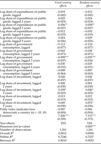
Table 1 presents the effect of government spending on income. We find that it takes up to three years before there is a significant positive effect on income from all our government spending variables. A 10 per cent increase in the share of expenditures on public goods significantly increases income by 0.6 per cent after three years. The steady state effect of the share of expenditures on public goods is positive but not statistically significant since it includes the sum of all the coefficients from years when government spending does not significantly affect income. Total government spending, which includes government consumption and government investment, leads to a net decline in income. This implies that the type of government spending is more important than aggregate spending in raising the purchasing power of consumers.
Income and the share of public good spending using log of three-year moving average of household final consumption as the dependent variable

Notes:***p<0.01, **p < 0.05, *p < 0.1. Huber–White standard errors in brackets clustered at the country level.
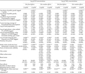
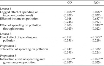
From table 2, there is a positive effect of income on our measures of consumption pollution in the fixed effects (FE) specification. A 10 per cent increase in income raises NO2 by 3 to 7 per cent but it has an insignificant effect on CO. Combining the effect of the share of expenditures on public goods from table 1 and the results from table 2, we find that the effect of the share of expenditures on public goods on pollution through income is positive but only significant for NO2, as summarized in table 3. Thus, our findings provide some support for Lemma 1.
Pollution and the share of public good spending (dependent variables in logs)

Notes: ***p < 0.01, **p < 0.05, *p<0.1. Huber–White standard errors in brackets clustered at the country level.
Summary of tests for selected propositions and lemmas

Notes: ***p<0.05, **p < 0.1, *p < 0.20. Standard errors for parts of Lemma 1, Lemma 2 and Proposition 2 are calculated using the delta method. Note that the lagged effect of spending composition on income is at the country level and is equivalent across all the different types of pollutants. Also, the fixed effects point estimates and standard errors were used in the calculation.
The parameter associated with the share of expenditures on public goods for our pollutants is positive but statistically insignificant in most of our specifications. However, we obtain a negative and statistically significant coefficient estimate for the interaction variable that is consistent across all FE models. Exclusion of the interaction variable amounts to omitted variable bias.Footnote 16 The higher the measure of democracy, the more effective an increase in the share of expenditures on public goods is in reducing consumption pollution which supports Proposition 3. At the mean quality of democracy, we find that a 10 per cent increase in the share of expenditures of public goods reduces all pollutants but it is only significant for NO2 where it declines by 3.6 per cent.Footnote 17 The direct effect may be interpreted as the reduction in consumption pollution due to an increase in regulatory stringency which implies some support for Lemma 2.
Since the direct effect of the share of expenditures on public goods reduces pollution but its effect through income is positive but smaller, the overall effect reduces consumption pollution conditional on the quality of democracy as shown in table 3. At the mean level of democratic quality, we find that a 10 per cent increase in the share of expenditures on public goods reduces both pollutants but it is only significant for NO2 where it declines by approximately 3.2 per cent. Thus, there is some support for Proposition 2 where expenditures on public goods such as spending on environmental regulations coupled with a reduction in expenditures for private goods such as subsidies to fossil fuel production reduces consumption pollution.
Our theoretical model also provides a plausible explanation for the relative insignificance of the coefficients for the other pollutants. From our theory, there are more requirements needed for a change in the composition of public spending to negatively affect pollution such as an inelastic demand for the good, low marginal income from a change in public spending composition and relatively low marginal product of expenditures on public goods as outlined in conditions (C1)–(C3). If these conditions do not hold, the effect of the composition of spending through regulations may not be strong enough to overcome the effect through income.
We simulate the effect of a change in democratic quality and fiscal spending composition in two countries in our sample: South Korea and the UK. Given our sample data periods, South Korea had a polity score and share of expenditures on public goods of 6 and 38 per cent, respectively while for the UK it was 10 and 60 per cent, respectively. If South Korea changed its share of expenditures on public goods to the same level as the UK, holding polity score constant, CO and NO2 would decline by 3.5 and 5.6 per cent, respectively. If South Korea also changed its governance level to match that of the UK, there would be an additional decline in pollution by 12–14 per cent.
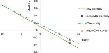
We calculate how the elasticity of pollution from a change in expenditures on public goods varies at different levels of the polity variable for the FE model and plot it in figure 1. As countries are more democratic, the elasticity of pollution given a change in the share of expenditures on public goods is more negative and more elastic. For countries considered very democratic, the effect of expenditures on public goods through environmental regulations dominates the effect through income but for autocratic countries the income effect dominates instead. Interestingly, the elasticity is only significant at the extreme ends of the political spectrum (very democratic or very autocratic). For CO, the elasticity is significant for autocratic countries with measures of polity between −10 and 0. For NO2 the elasticity is significant for measures of polity between −10 and −2 as well as 7–10 but insignificant elsewhere.
Elasticity of pollution conditional on the polity level

Not only do our results corroborate some of the existing specific regional studies in the literature but we also generalize the results to other political systems. Recent studies show a significant relationship between fiscal spending composition and consumption pollutants for the top economies in Europe and the USA (López and Palacios, Reference López and Palacios2014; Islam and López, Reference Islam and López2015) but not for the rest of the world (López et al., Reference López, Galinato and Islam2009). Using a data set with developed and developing countries, we show that ignoring the interaction between polity and government spending leads to omitted variable bias, masking the true impact of public spending on consumption pollution.
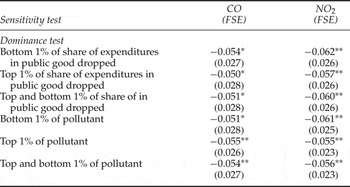
Our main variable of interest is the interaction variable between polity and the share of expenditure on public goods. We check if the results are robust to sample outliers. We consider the possibility that outliers may be driving the results. Therefore we omit the bottom 1 per cent and top 1 per cent of observations of the share of expenditures on public goods in the sample and re-estimate the results. We also repeat the estimations by dropping the bottom 1 per cent and top 1 per cent of the pollutant. As indicated in table 4, these sample alterations do not affect the coefficients of the interaction of the share of expenditures on public goods and polity in our specifications.
Dominance tests of the fixed-effects estimates on the effect of share of government expenditures on public goods × polity on pollutants

Notes: *Significant at 10%; **significant at 5%.
5. Conclusions
This paper elucidates the mechanisms by which government spending affects consumption-based pollution. Our theoretical model shows that expenditures on public goods that alleviate market failure have countervailing effects on consumption pollution through an income channel and an environmental regulation channel. Examples of expenditures on public goods include low-income household subsidies to reduce credit market constraints in the education sector and environmental protection spending to reduce pollution externalities More government expenditures on public goods raise income which increases consumption and corresponding pollution levels; however, it also increases regulation stringency, which decreases consumption pollution. Conditional on a country being democratic, government spending on expenditures on public goods is likely to reduce consumption pollution because of a larger regulatory effect than income. However, the opposite holds for autocratic countries. We verify our theoretical propositions by showing that CO and NO2 decrease as more of the share of government expenditures go towards alleviating market failure for countries that are democratic. However, the opposite holds for autocratic countries.
The results have important policy implications because during times of recession when countries increase their share of expenditures on public goods, we are able to predict its impact on consumption pollution. When countries similar to the USA and members of the European Union expand spending on goods that alleviate market failure, such as education, health and public goods, it could also have a positive unexpected effect: better environmental quality through a reduction in consumption pollution. However, in countries such as China, a similar change in fiscal policy would result in an unintended consequence: deteriorating environmental quality as shown by an increase in consumption pollution. By understanding these potential effects, one could design policies to either enhance any potential positive environmental benefit or mitigate any potential adverse environmental degradation.
Supplementary material and methods
To view supplementary material for this article, please visit https://doi.org/10.1017/S1355770X17000237.