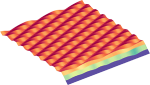



1. Introduction
Fluid flows that accompany solid–liquid phase transition are ubiquitous in both the natural and engineering environments (Epstein & Cheung Reference Epstein and Cheung1983; Glicksman, Coriell & McFadden Reference Glicksman, Coriell and McFadden1986; Huppert Reference Huppert1986; Worster Reference Worster2000; Hewitt Reference Hewitt2020). The generation of fluid motions in such situations is due to buoyancy forces generated by thermal and compositional gradients arising during solidification (Davis, Müller & Dietsche Reference Davis, Müller and Dietsche1984; Dietsche & Müller Reference Dietsche and Müller1985; Wettlaufer, Worster & Huppert Reference Wettlaufer, Worster and Huppert1997; Worster Reference Worster1997; Davies Wykes et al. Reference Davies Wykes, Huang, Hajjar and Ristroph2018) and/or externally imposed mean shear (Delves Reference Delves1968, Reference Delves1971; Gilpin, Hirata & Cheng Reference Gilpin, Hirata and Cheng1980; Coriell et al. Reference Coriell, McFadden, Boisvert and Sekerka1984; Forth & Wheeler Reference Forth and Wheeler1989; Feltham & Worster Reference Feltham and Worster1999; Neufeld & Wettlaufer Reference Neufeld and Wettlaufer2008a,Reference Neufeld and Wettlauferb; Ramudu et al. Reference Ramudu, Hirsh, Olson and Gnanadesikan2016; Bushuk et al. Reference Bushuk, Holland, Stanton, Stern and Gray2019). In this study, we are concerned with the shear- and buoyancy-driven flow of a pure melt over its evolving solid phase.
Some of the first systematic investigations into the effects of a phase boundary on convective motions in a pure melt are those of Davis et al. (Reference Davis, Müller and Dietsche1984) and Dietsche & Müller (Reference Dietsche and Müller1985). Davis et al. (Reference Davis, Müller and Dietsche1984) studied fluid motions and pattern formation in Rayleigh–Bénard convection (RBC) over a phase-changing boundary using experiments and weakly nonlinear stability theory. The primary focus of their study was on identifying different regimes in which roll, hexagonal and mixed patterns appeared at the phase boundary. Some of the key results from their study are: (i) both the critical Rayleigh number ( $Ra_c$) and the critical wavenumber (
 $k_c$) for the onset of convection decrease monotonically with
 $\mathcal{A}$, where
 $\mathcal{A}$ is the ratio of the initial thickness of the solid layer to the initial thickness of the liquid layer, and asymptote to constant values for large values of
 $\mathcal{A}$; (ii) hexagonal and roll patterns on the phase boundary are observed when
 $\mathcal{A}$ is large and small, respectively; and (iii) the onset of hexagonal convection is accompanied by a jump in the heat flux and thereby in the mean position of the phase boundary. The subsequent experimental study of Dietsche & Müller (Reference Dietsche and Müller1985) confirmed the predictions of jump in the phase-boundary position and the existence of strong hysteresis behaviour near the onset of convection. They also explored the different interfacial patterns that emerged with increasing
 $Ra$.
Recent studies on the coupled convection-phase-change problem have focused on  $Ra \gg Ra_c$. Esfahani et al. (Reference Esfahani, Hirata, Berti and Calzavarini2018) numerically studied the interactions between a melting isothermal solid phase and convective motions in the underlying liquid phase in two and three dimensions. A key result from their study is that the dimensionless heat flux (
 $\mathcal {N}$) is only weakly dependent on the Stefan number (
 $\mathcal {S}$), which is defined as the ratio of latent heat of fusion to the specific heat content of a material and quantifies the pace at which phase change proceeds. Using a similar configuration in two dimensions, Favier, Purseed & Duchemin (Reference Favier, Purseed and Duchemin2019) systematically explored the different transitions in the convection cell structure as the solid and liquid phases evolved. They showed that owing to the presence of the phase boundary, the flow remains steady even at large
 $Ra$. This results in higher heat transport than in the classical RBC in two dimensions, where the flow becomes unsteady at
 $Ra \approx 7.5 \times 10^5$ (Toppaladoddi, Succi & Wettlaufer Reference Toppaladoddi, Succi and Wettlaufer2015a). Purseed et al. (Reference Purseed, Favier, Duchemin and Hester2020) considered a more general situation where the melting point of the solid lies between the temperatures imposed at the upper and lower boundaries and studied the bistability close to the onset of convection which was first predicted by Davis et al. (Reference Davis, Müller and Dietsche1984).
From the studies of thermal convection over phase boundaries it can be concluded that when the temperature of the upper boundary is less than the melting point, the phase boundary develops steady patterns, polygons, rolls or a mix of both, due to steady convection cells for up to  $Ra = O(10^8)$. The introduction of a mean shear flow, however, introduces additional interesting effects. The effects of both shear- and buoyancy-driven flows on the directional solidification of two-component melts have been extensively studied in the past. A detailed discussion of those studies can be found in Toppaladoddi & Wettlaufer (Reference Toppaladoddi and Wettlaufer2019).
Some of the early systematic studies on shear flows over phase boundaries are those of Hirata, Gilpin & Cheng (Reference Hirata, Gilpin and Cheng1979a); Hirata et al. (Reference Hirata, Gilpin, Cheng and Gates1979b) and Gilpin et al. (Reference Gilpin, Hirata and Cheng1980). Here, we focus on the work of Gilpin et al. (Reference Gilpin, Hirata and Cheng1980) because of certain features observed in their experiments. Gilpin et al. (Reference Gilpin, Hirata and Cheng1980) considered a turbulent boundary-layer flow over a layer of ice. At the initial instant, a groove was melted into the ice layer to introduce a perturbation at the ice–water interface. Subsequently, the effects of the shear flow on the growth of this perturbation was studied. They observed that under certain conditions, the perturbation grew and propagated downstream, leading to the formation of a ‘rippled’ surface. This led to an increase in the heat transfer rate by as much as 30–60 % compared with a flat surface. Gilpin et al. (Reference Gilpin, Hirata and Cheng1980) attributed these observations to the effects of shear. However, because of the 4  $^{\circ }$C density maximum of water, the layer of water overlying the ice surface was unstably stratified. Hence, their observations were due to the combined effects of mean shear and buoyancy. This was recognised by Toppaladoddi & Wettlaufer (Reference Toppaladoddi and Wettlaufer2019), who reanalysed the velocity profiles from the experiments of Gilpin et al. (Reference Gilpin, Hirata and Cheng1980) and showed that these are described better by the Monin–Obukhov theory than the classical law of the wall (Monin & Yaglom Reference Monin and Yaglom1971). They also showed that the Obukhov length scale that emerged from these measurements was negative, implying that the column of liquid was unstably stratified. Furthermore, Toppaladoddi & Wettlaufer (Reference Toppaladoddi and Wettlaufer2019) studied the stability of a phase boundary with a Rayleigh–Bénard–Couette flow over it and showed that buoyancy destabilises the phase boundary, whereas shear stabilises it. They also found that for certain values of
 $Pe$, travelling waves are generated at the phase boundary. This tendency of buoyancy to cause large ‘deformations’ to a phase boundary is also present in the turbulent regime: Couston et al. (Reference Couston, Hester, Favier, Taylor, Holland and Jenkins2020), who recently studied stably, neutrally and unstably stratified shear flows over a phase boundary using direct numerical simulations (DNS), found that when the flow is unstably stratified, the ‘channels’ and ‘keels’ that are formed at the interface interact strongly with the underlying flow.
Here, motivated by the experiments of Gilpin et al. (Reference Gilpin, Hirata and Cheng1980), we study the dynamics of an unstably stratified shear flow over a phase boundary in the laminar regime in two dimensions. Specifically, we use a combination of the lattice Boltzmann method (LBM) and the enthalpy method to simulate Rayleigh–Bénard–Poiseuille flow over a phase boundary and study their interactions. The present study is also a qualitative continuation of the work described in Toppaladoddi & Wettlaufer (Reference Toppaladoddi and Wettlaufer2019) into the nonlinear regime.
2. Governing equations
The horizontally periodic domain used in this study is shown in figure 1. The cell height and length are  $L_z$ and
 $L_x$, respectively. The aspect ratio of the domain is defined as
 $\varGamma = L_x/L_z$. Initially, the phase boundary is planar at
 $z = h_0$ and the fluid occupies the region
 $0 \le z \le h_0$. The initial thickness of the solid layer is
 $d_0 = L_z - h_0$. The bottom plate is maintained at a temperature
 $T_h$ and the top plate is maintained at
 $T_c$. The melting point of the solid phase is
 $T_m$ and the temperature boundary conditions are such that
 $T_c < T_m < T_h$. We also have a fully developed Poiseuille flow in the liquid region starting from the initial instant. As the flow develops, the initially flat phase boundary may grow/melt resulting in a deformed interface. The location of the phase boundary and the thickness of the solid layer at any time instant
 $t > 0$ are denoted by
 $h(x,t)$ and
 $d(x,t)$, respectively. Note that
 $h(x,t) + d(x,t) = L_z$.
Schematic of the horizontally periodic domain considered here. The initial thicknesses of the liquid and solid layers are  $h_0$ and
 $d_0 = L_z - h_0$, respectively. The temperature boundary conditions are such that
 $T_c < T_m < T_h$. No-slip and no-penetration boundary conditions for the velocity field are imposed at the bottom boundary and the phase boundary. The temperature fields in the liquid and solid regions at the initial instant vary only with height and the horizontal velocity profile in the liquid region is parabolic.

The governing equations in the different regions are as follows.
2.1. Liquid
The mass, momentum and heat balance equations are
 \begin{gather} \boldsymbol{\nabla} \boldsymbol{\cdot} \boldsymbol{u} = 0, \end{gather}
 \begin{gather}\frac{\partial \boldsymbol{u}}{\partial t} + \boldsymbol{u} \boldsymbol{\cdot} \boldsymbol{\nabla} \boldsymbol{u} ={-}\frac{1}{\rho_0} \boldsymbol{\nabla} p + g \alpha (T_l-T_m) \boldsymbol{\hat{z}} + \nu \nabla^2 \boldsymbol{u}, \end{gather}
 \begin{gather}\frac{\partial T_l}{\partial t} + \boldsymbol{u} \boldsymbol{\cdot} \boldsymbol{\nabla} T_l = \kappa \nabla^2 T_l, \end{gather}
respectively. Here,  $\boldsymbol {u}(\boldsymbol {x},t) = (u, w)$ is the two-dimensional velocity field,
 $\rho _0$ is the reference density,
 $p(\boldsymbol {x},t)$ is the pressure field,
 $g$ is acceleration due to gravity,
 $\alpha$ is the thermal expansion coefficient,
 $T_l(\boldsymbol {x},t)$ is the temperature field in the liquid,
 $\boldsymbol {\hat {z}}$ is the unit vector along the vertical,
 $\nu$ is the kinematic viscosity and
 $\kappa$ is the thermal diffusivity. We assume the liquid and solid phases have the same density (
 $\rho _0$) and thermal diffusivity (
 $\kappa$).
2.2. Solid
The temperature field in the solid,  $T_s(\boldsymbol {x},t)$, evolves according to the diffusion equation
 \begin{equation} \frac{\partial T_s}{\partial t} = \kappa \nabla^2 T_s.\end{equation}
2.3. Evolution of the phase boundary
To track the location of the phase boundary, we need an additional equation for its evolution, which is given by the Stefan condition (Worster Reference Worster2000):
 \begin{equation} \rho_0 L_s v_n = \boldsymbol{n} \boldsymbol{\cdot} [\boldsymbol{q_s} - \boldsymbol{q_l}]_{z = h}.\end{equation}
Here,  $L_s$ is the latent heat of fusion,
 $v_n$ is the normal component of growth rate of the solid phase,
 $\boldsymbol {n}$ is the unit normal pointing into the liquid,
 $\boldsymbol {q_s}$ and
 $\boldsymbol {q_l}$ are the heat fluxes away from the phase boundary into the solid and towards the phase boundary from the liquid, respectively.
2.4. Boundary conditions
We impose Dirichlet conditions on temperature at the bottom and top boundaries of the domain such that
 \begin{equation} T_l(z=0,t) = T_h \quad \mbox{and} \quad T_s(z = L_z,t) = T_c. \end{equation}
And, at the phase boundary, the temperature is the equilibrium temperature
 \begin{equation} T_l(z=h,t) = T_s(z = h,t) = T_m. \end{equation}
For the velocity field in the liquid region, we impose no-slip and no-penetration conditions at the bottom boundary and the phase boundary such that
 \begin{gather} u(z = 0, t) = w(z = 0, t) = 0, \end{gather}
 \begin{gather}\boldsymbol{u} \boldsymbol{\cdot} \boldsymbol{n} = \boldsymbol{u} \boldsymbol{\cdot} \boldsymbol{t} = 0 \quad \mbox{at } z = h(x,t), \end{gather}
where  $\boldsymbol {t}$ is the unit tangent at the phase boundary. We also impose periodic boundary conditions for the temperature and velocity fields at
 $x = 0$ and
 $x = L_x$.
2.5. Non-dimensional equations
To non-dimensionalise the equations of motion, we choose the initial centreline velocity of the Poiseuille profile in the liquid region,  $U_0$, as the velocity scale,
 $h_0$ as the length scale,
 $t_0 = h_0^2/\kappa$ as the time scale,
 $p_0 = \rho _0 U_0 \kappa /h_0$ as the pressure scale and
 ${\rm \Delta} T = T_h - T_m$ as the temperature scale. Using these we obtain the dimensionless versions of (2.1)–(2.5) as
 \begin{gather} \boldsymbol{\nabla} \boldsymbol{\cdot} \boldsymbol{u} = 0, \end{gather}
 \begin{gather}\frac{\partial \boldsymbol{u}}{\partial t} + Pe (\boldsymbol{u} \boldsymbol{\cdot} \boldsymbol{\nabla} \boldsymbol{u}) ={-}\boldsymbol{\nabla} p + \frac{Ra Pr}{Pe} \theta_l \boldsymbol{\hat{z}} + Pr \nabla^2 \boldsymbol{u}, \end{gather}
 \begin{gather}\frac{\partial \theta_l}{\partial t} + Pe (\boldsymbol{u} \boldsymbol{\cdot} \boldsymbol{\nabla} \theta_l ) = \nabla^2 \theta_l, \end{gather}
 \begin{gather}\frac{\partial \theta_s}{\partial t} = \nabla^2 \theta_s, \end{gather}
and
 \begin{equation} v_n = \frac{1}{\varLambda \mathcal{S}} [\boldsymbol{n} \boldsymbol{\cdot} (\boldsymbol{q_s} - \boldsymbol{q_l})]_{z = h},\end{equation}
where
 \begin{equation} \theta_l = \frac{T_l - T_m}{{\rm \Delta} T} \quad \mbox{and} \quad \theta_s = \frac{T_s - T_m}{{\rm \Delta} T}. \end{equation}
Here, we have maintained the pre-scaled notation for  $\boldsymbol {u}, t$ and
 $\boldsymbol {x}$ for simplicity. There are five governing parameters, which are
 \begin{gather} Ra = \frac{g \alpha {\rm \Delta} T h_0^3}{\nu \kappa}, \quad Pe = \frac{U_0 h_0}{\kappa}, \quad Pr = \frac{\nu}{\kappa}, \end{gather}
 \begin{gather}\mathcal{S} = \frac{L_s}{C_p (T_m-T_c)} \quad \mbox{and} \quad \varLambda = \frac{(T_m - T_c)}{{\rm \Delta} T}, \end{gather}
where  $C_p$ is the specific heat of the solid phase and
 $\varLambda$ denotes the ratio of temperature differences in the solid and liquid regions.
The non-dimensional versions of the boundary conditions are
 \begin{gather} \theta_l(z = 0, t) = \theta_h = 1 \quad \mbox{and} \quad \theta_s(z = L_z, t) = \theta_c ={-}\varLambda, \end{gather}
 \begin{gather}\theta_s(z = h, t) = \theta_l(z = h, t) = \theta_m = 0, \end{gather}
 \begin{gather}u(z = 0, t) = w(z = 0, t) = 0 \quad \mbox{and} \end{gather}
 \begin{gather}\boldsymbol{u} \boldsymbol{\cdot} \boldsymbol{n} = \boldsymbol{u} \boldsymbol{\cdot} \boldsymbol{t} = 0 \quad \mbox{at } z = h(x,t). \end{gather}
2.6. Initial conditions
At the initial instant, the temperature profiles in the liquid and solid regions are given by
 \begin{equation} \theta_l^{(0)}(z) = 1-z, \end{equation}
and
 \begin{equation} \theta_s^{(0)}(z) = \frac{\varLambda}{d_0} (1-z). \end{equation}
In addition, we demand that the heat fluxes at the phase boundary balance at the initial instant (see (2.14)), giving
 \begin{equation} \frac{\textrm{d} \theta_l^{(0)}}{\textrm{d} z} = \frac{\textrm{d} \theta_s^{(0)}}{\textrm{d} z} \quad \mbox{at } z = 1. \end{equation}
This gives
 \begin{equation} \varLambda = d_0. \end{equation}
2.7. Heat transport
The response of the system is quantified using the dimensionless heat flux, which is the Nusselt number, defined as
 \begin{equation} Nu(t) = \left. -\frac{1}{L_x} \int_0^{L_x} \left(\frac{\partial T_l}{\partial z}\right) \, {\textrm{d} x} \right/ \left[\frac{{\rm \Delta} T}{\bar{h}(t)}\right] \quad \mbox{at } z = 0. \end{equation}
Here,  $\bar {h}(t)$ denotes the instantaneous horizontally averaged thickness of the liquid layer. After the dynamics have reached a stationary state, the horizontally and temporally averaged Nusselt number is calculated as
 \begin{equation} \mathcal{N} = \frac{1}{T} \int_{t_0}^{t_0+T} Nu(t) \, \textrm{d} t. \end{equation}
We also define the horizontally and temporally averaged liquid height as
 \begin{equation} h_m = \frac{1}{T} \int_{t_0}^{t_0+T} \bar{h}(t) \, \textrm{d} t, \end{equation}
and the effective  $Ra$ based on
 $h_m$ as
 \begin{equation} Ra_e = \frac{g \alpha {\rm \Delta} T h_m^3}{\nu \kappa}.\end{equation}
The results from this study are discussed in terms of either  $Ra$ or
 $Ra_e$.
3. Numerical method
To numerically solve the equations of motion and the boundary conditions, we combine the LBM (Benzi, Succi & Vergassola Reference Benzi, Succi and Vergassola1992; Chen & Doolen Reference Chen and Doolen1998) with the enthalpy method (Voller, Cross & Markatos Reference Voller, Cross and Markatos1987). In the enthalpy method, the total enthalpy is split into specific and latent heat contributions and the regions that undergo phase change are tracked through the changes in the latent heat content of those regions (Voller et al. Reference Voller, Cross and Markatos1987). A phase variable  $\phi (\boldsymbol {x},t)$, which represents the liquid fraction field, is introduced to follow the evolution of the different phases. A grid point
 $\boldsymbol {x} = (x_i,z_j)$ is deemed to be solid or liquid depending on whether
 $\phi (\boldsymbol {x}) \le \phi _0$ or
 $\phi (\boldsymbol {x}) > \phi _0$, where
 $\phi _0 \in (0, 1)$ denotes a chosen threshold value. The choice of
 $\phi _0$ is arbitrary, but choosing a large value effectively increases the latent heat of fusion for the following reason. The change in the nature of a grid point (solid to liquid, or vice versa) involves a change in the latent heat of fusion. A smaller value of
 $\phi _0$ requires a smaller amount of heat of fusion to be provided to effect a change from solid to liquid grid point when compared with a higher value of
 $\phi _0$. In this study, we choose
 $\phi _0 = 0.5$.
The principal advantage of the enthalpy method is that the phase boundary is not explicitly tracked, resulting in less onerous requirements for grid resolution when compared with other methods. The details of the enthalpy method can be found in Voller & Cross (Reference Voller and Cross1981) and Voller et al. (Reference Voller, Cross and Markatos1987) and its implementation for conduction- and convection-driven phase-change problems using LBM can be found in Jiaung, Ho & Kuo (Reference Jiaung, Ho and Kuo2001) and Huber et al. (Reference Huber, Parmigiani, Chopard, Manga and Bachmann2008), respectively. For our study, we use the scheme of Huber et al. (Reference Huber, Parmigiani, Chopard, Manga and Bachmann2008). Further details are provided in Appendix A.
For the fluid flow, we use the D2Q9 (Succi Reference Succi2001) and D2Q5 (Latt Reference Latt2007) lattice models for the velocity and temperature distribution functions, respectively. No-slip and no-penetration boundary conditions for the velocity field are imposed using the mid-grid bounceback scheme (Succi Reference Succi2001), which is known to conserve mass for flows over complex geometries in the high  $Ra$ and
 $Re$ regimes (Toppaladoddi Reference Toppaladoddi2017). The Dirichlet boundary conditions for the temperature field are imposed by requiring that the temperature distribution functions at the boundaries are the corresponding equilibrium distribution functions.
The flow simulated by the LBM is weakly compressible and the equation of state is the ideal gas law. Hence, it is difficult to maintain significant pressure gradients in the flow (Succi Reference Succi2001). For these reasons, a body force  $G$, which mimics an applied pressure gradient, is introduced in the evolution equation for the velocity distribution functions. In dimensional units, the centreline velocity in plane Poiseuille flow is given by
 \begin{equation} U_0 = \frac{|\boldsymbol{\nabla} p_0| h_0^2}{8 \rho_0 \nu},\end{equation}
where  $|\boldsymbol {\nabla } p_0|$ is the constant pressure gradient. Choosing a value of
 $U_0$,
 $G\ (= |\boldsymbol {\nabla } p_0|)$ is determined using (3.1) and then used to drive the flow in the LBM. Further details on the implementation can be found in Toppaladoddi (Reference Toppaladoddi2017).
Our numerical code has been rigorously validated against spectral methods for both RBC (Toppaladoddi et al. Reference Toppaladoddi, Succi and Wettlaufer2015a) and Poiseuille flow (Toppaladoddi, Succi & Wettlaufer Reference Toppaladoddi, Succi and Wettlaufer2015b). We have also validated the code for transient, conduction-driven melting problems against analytical solutions (Toppaladoddi Reference Toppaladoddi2017). Further validation is presented in the following sections where we compare some of our results for pure convection over a phase boundary with those that exist in the literature.
4. Results
4.1. RBC over a phase boundary
Here, we present results from our simulations for purely convective flow over a phase boundary. The discussion of these results serves the following two main purposes. First, it allows us to compare our results with the previous experiments and DNS studies and, hence, assess the accuracy of our formulation and simulation methods. Second, it provides a natural comparison point for our later discussion of the effects of mean shear on the convective motions and on the evolution of the phase boundary.
The resolution used in the simulations varies with  $Ra$, e.g. for
 $Ra = 2.15 \times 10^3$ we use
 $400 \times 100$ grid points and for
 $Ra = 10^6$ we use
 $1200 \times 300$ grid points. These resolutions are such that there are at least nine grid points in each boundary layer. Furthermore, we fix
 $Pr = 1$ and
 $h_0 = d_0 = 1$ for all simulations.
4.1.1. Onset of thermal convection
To study the onset of convection, we perform simulations for  $Ra \in [1470, 1600]$,
 $\mathcal {S} = 5.82$ and
 $\varGamma = 10$. The value of
 $\mathcal {S}$ is chosen to match the experimental conditions of Dietsche & Müller (Reference Dietsche and Müller1985), who used cyclohexane as the working fluid, and the large value of
 $\varGamma$ is chosen to ensure any finite-size effects are minimised. The
 $Pr$ for cyclohexane is
 $17.6$ (Dietsche & Müller Reference Dietsche and Müller1985), but we use
 $Pr = 1$ in our simulations. This choice does not affect the onset of convection as
 $Ra_c$ is independent of
 $Pr$ for this system (Davis et al. Reference Davis, Müller and Dietsche1984; Toppaladoddi & Wettlaufer Reference Toppaladoddi and Wettlaufer2019).
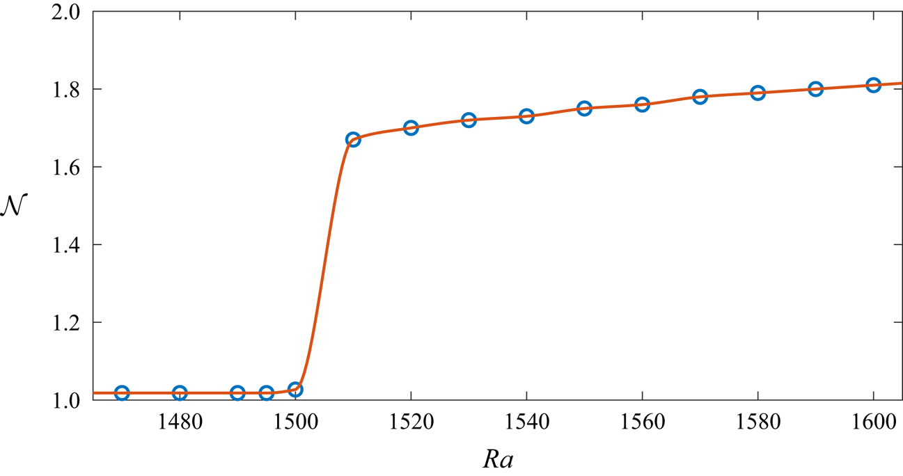
Figure 2 shows  $\mathcal {N}(Ra)$ for
 $Ra \in [1470, 1600]$. There is a jump in
 $\mathcal {N}$ at the onset of convection, which is at
 $Ra \approx 1510$. The jump in
 $\mathcal {N}$ is related to the jump in the interface position and the onset of convection for the following reason. At the initial instant, the temperature gradients in both the solid and liquid layers are such that the heat fluxes in (2.14) are equal. This remains true for all
 $Ra < Ra_c$ and, hence, there is no change in the position of the interface. At
 $Ra = Ra_c$, the heat flux in the liquid layer increases due to the onset of convective motion. As a result of this heat-flux imbalance, a part of the solid phase melts and the interface reaches a new position, resulting in more vigorous convection (Davis et al. Reference Davis, Müller and Dietsche1984). This is a positive feedback loop and a steady state is reached when the mean thickness of the solid phase is such that the balance in the heat fluxes at the interface is restored again.
Plot of  $\mathcal {N}(Ra)$ for
 $Ra \in [1470, 1600]$,
 $Pr =1$ and
 $\mathcal {S} = 5.82$. The critical
 $Ra$ is
 $Ra_c \approx 1510$.

The jump behaviour is in contrast to what happens near  $Ra_c$ in the classical RBC (Chandrasekhar Reference Chandrasekhar2013) and is in good agreement with the analysis of Davis et al. (Reference Davis, Müller and Dietsche1984), who predicted a subcritical bifurcation at
 $Ra = Ra_c$. Similar behaviour at
 $Ra = Ra_c$ has been reported in previous experiments (Dietsche & Müller Reference Dietsche and Müller1985) and DNS studies (Esfahani et al. Reference Esfahani, Hirata, Berti and Calzavarini2018; Purseed et al. Reference Purseed, Favier, Duchemin and Hester2020).
Figure 3 shows the contours of steady-state vertical velocity field for  $Ra = 1510$. We can calculate the critical wavenumber from figure 3, noting that there are nine pairs of counter-rotating cells. This gives the dimensionless wavelength as
 $\lambda = 20/9 \approx 2.22$ and the critical wavenumber as
 $k_c = 2 {\rm \pi}/ \lambda \approx 2.83$. These values are in excellent agreement with
 $Ra_c = 1493$ and
 $k_c = 2.82$ from the linear stability calculations of Davis et al. (Reference Davis, Müller and Dietsche1984).
Contours of steady-state vertical-velocity field for  $Ra = 1510$. The solid phase is shown in white. The velocity is non-dimensionalised by the buoyancy velocity scale
 $\sqrt {g \alpha {\rm \Delta} T h_0}$.

4.1.2. Thermal convection for larger  $Ra$

Before exploring the combined effects of shear and buoyancy on the evolution of the phase boundary, we investigate the effects of pure thermal convection for  $Ra \in [2.15 \times 10^3, 10^6]$. The simulation results reported in the remainder of this paper are for
 $\mathcal {S} = 1$, except in §4.2.5, and
 $\varGamma = 4$.
In figures 4(a) and 4(b) we show the time series for the horizontally averaged thickness of the liquid layer and the heat flux for  $Ra = 10^6$. The following observations can be made from these figures: (1) after an initial transient, both the thickness and the heat flux attain steady state; (2) the
 $Nu(t)$ time series exhibits oscillations before reaching the steady state. These oscillations are caused by the evolving convection cells, whose aspect ratio continuously changes before reaching the steady-state value. The effective
 $Ra$ for this case is
 $Ra_e \approx 6.5 \times 10^6$ and the steady state
 $\mathcal {N} = 16.27$, which is larger than
 $\mathcal {N} = 12.07$ for classical RBC (Johnston & Doering Reference Johnston and Doering2009). These results are in qualitative agreement with the findings of Favier et al. (Reference Favier, Purseed and Duchemin2019) and Purseed et al. (Reference Purseed, Favier, Duchemin and Hester2020). The increase in the heat flux compared with classical RBC is because the non-planar phase boundary ‘locks in’ the convection cells, thereby delaying the onset of unsteady convection (Favier et al. Reference Favier, Purseed and Duchemin2019). This is seen in figure 5, which shows a snapshot of the steady temperature field for
 $Ra = 10^6$. A close examination of the cusps at the phase boundary in figure 5 reveals that they have slightly different amplitudes.
Time series for the horizontally averaged (a) height of the liquid column and (b) heat flux for  $Ra = 10^6$.

Snapshot of the steady temperature field for  $Ra = 10^6$.

To understand the impact of the phase boundary on the dependence of heat flux on buoyancy forcing, we plot  $\mathcal {N}$ as a function of
 $Ra_e$ in figure 6. The data are described well by the power law
 $\mathcal {N} = 0.2 \times Ra_e^{0.285 \pm 0.009}$, which is obtained from a linear least-squares fit to the
 $\log \mathcal {N} - \log Ra_e$ data. The exponent
 $\beta = 0.285$, which is indistinguishable from
 $\beta = 2/7$, is in remarkable agreement with the findings of previous DNS studies of classical RBC (Johnston & Doering Reference Johnston and Doering2009; Toppaladoddi et al. Reference Toppaladoddi, Succi and Wettlaufer2015a). However, the prefactor here is larger than that in the classical RBC case. This is because it depends on the geometry of the boundaries (Toppaladoddi et al. Reference Toppaladoddi, Succi and Wettlaufer2015a). This effect on the prefactor has been reported by Favier et al. (Reference Favier, Purseed and Duchemin2019) as well, with
 $\beta \approx 0.27$ in their case.
Plot of  $\mathcal {N}$ as a function of
 $Ra_e$. The latter is calculated using (2.29). Symbols are data from simulations and the solid line is the fit
 $Nu = 0.2 \times Ra_e^{0.285 \pm 0.009}$. The error bars on the exponent represent the 95 % confidence interval. The inset shows the residuals from the fit. The curvature in the residual indicates that there is a weak deviation from the power-law fit.

Another feature that is absent in figure 6 is a discontinuity in the  $\mathcal {N}(Ra_e)$ data at around
 $Ra_e = 10^6$, which is due to a pattern competition instability observed in the classical RBC (Glazier et al. Reference Glazier, Segawa, Naert and Sano1999; Johnston & Doering Reference Johnston and Doering2009). This indicates that the phase boundary suppresses this instability. However, this does not rule out its appearance at a higher
 $Ra$.
In figure 7, we show our  $\mathcal {N}(Ra_e)$ data along with those from Purseed et al. (Reference Purseed, Favier, Duchemin and Hester2020), who had
 $\varGamma = 6$,
 $h_0 = 1.8$ and
 $\mathcal {S} = Pr = 1$ in their simulations. The agreement between the results shows that for a fixed
 $Pr$,
 $\mathcal {N}$ depends only on
 $Ra_e$ and does not appreciably depend on the initial conditions.
Comparison of  $\mathcal {N}(Ra_e)$ data with those from Purseed et al. (Reference Purseed, Favier, Duchemin and Hester2020), who had
 $\varGamma = 6$,
 $h_0 = 1.8$ and
 $\mathcal {S} = Pr = 1$ in their simulations. Circles are data points from the present study and diamonds are from Purseed et al. (Reference Purseed, Favier, Duchemin and Hester2020).

4.2. Rayleigh–Bénard–Poiseuille flow over a phase boundary
Having established consistency of our simulations with previous work on coupled convection and phase change, we now explore the effects of mean shear on both the convective motions and the evolution of the phase boundary. The range of  $Pe$ used in this study is
 $Pe \in [0,50]$. The simulations of Rayleigh–Bénard–Poiseuille flow are as equally well resolved as our simulations of RBC over a phase boundary, with at least nine grid points in each boundary layer.
4.2.1. Mean height of the liquid layer
We first consider the combined effects of mean shear and buoyancy on the mean height of the liquid layer. In figure 8,  $h_m$ is shown as a function of
 $Ra$ for the different
 $Pe$ considered. The following observations can be made from the figure: (i) with increasing
 $Ra$, the variation in
 $h_m$ for the different
 $Pe$ decreases; (ii) for
 $Pe = 40$ and
 $50$ and the lowest
 $Ra$, there is negligible melting of the phase boundary, indicating there is no bifurcation to steady convection; and (iii) for a fixed
 $Ra \ge 2.15 \times 10^4$, the changes in
 $h_m$ are not monotonic with
 $Pe$. These observations indicate that the interplay between the shear flow and convection has substantial effects on the evolution of the phase boundary.
Mean height of the liquid layer,  $h_m$, as a function of
 $Ra$ for the different values of
 $Pe$.

4.2.2. Heat transport
To understand these effects, we consider the impact of mean shear and buoyancy on the transport of heat. In figure 9 we show the temperature fields for  $Ra = 2.15 \times 10^3$ and (a)
 $Pe = 10$ and (b)
 $Pe = 50$ at
 $t = 49.84$. The deformation of the phase boundary in figure 9(a) is caused by the convection cells. The mean shear flow has a considerable effect on the convective motions: for
 $Pe = 10$ the convection cells are slightly distorted, but for
 $Pe = 50$ the convective motions disappear completely.
Temperature fields for  $Ra = 2.15 \times 10^3$ and (a)
 $Pe = 10$ and (b)
 $Pe = 50$ at
 $t = 49.84$. Convective motions are suppressed for
 $Pe = 50$.

The effects of the mean shear on convective motion can be seen more clearly by considering its effects on  $Ra_c$, which is shown in figure 10 and on the heat transport, which is shown in figure 11. The
 $Ra_c$ is a monotonically increasing function of
 $Pe$, with the solid line in figure 10 showing a least-squares fit to the data. The behaviour of
 $\mathcal {N}$ with
 $Ra$ and
 $Pe$ in figure 11 is qualitatively similar to that of
 $h_m$ (figure 8). To obtain a more complete understanding, the relative effects of mean shear and buoyancy have to be considered.
Critical Rayleigh number for the onset of convection as a function of  $Pe$. The circles are data from simulations and the solid line is the least-squares fit. For
 $Pe = 0$,
 $\varGamma = 10$ and for
 $Pe > 0$,
 $\varGamma = 4$.

Plot of  $\mathcal {N}$ as a function of
 $Ra$ for the different
 $Pe$.

To quantify the relative strengths of buoyancy and mean shear, we introduce a bulk Richardson number, defined as (Chandrasekhar Reference Chandrasekhar2013)
 \begin{equation} Ri_b = \frac{g \alpha {\rm \Delta} T h_0}{U_0^2} = \frac{Ra \cdot Pr}{Pe^2} \end{equation}
and use it to study the changes in  $\mathcal {N}$ for different values of
 $Ra$ and
 $Pe$. In figure 12 we show the dependence of
 $\mathcal {N}$ on
 $Ri_b$ for the different
 $Pe > 0$. For
 $Ri_b = O(1)$, the mean shear dominates and hence the heat transport is only due to conduction. However, for
 $Ri_b \gg 1$ buoyancy dominates and the values of
 $\mathcal {N}$ are close to those for purely convective flow (see figure 11). For a fixed value of
 $Ra$,
 $\mathcal {N}$ does not increase monotonically with decreasing
 $Pe$ because the changes in the value of
 $h_m$ and, hence,
 $Ra_e$ is not monotonic with
 $Pe$.
Plot of  $\mathcal {N}$ as a function of
 $Ri_b$ for the different
 $Pe$. For each
 $Pe$, the simulations cover the
 $Ra$ range
 $Ra \in [2.15 \times 10^3, 10^6]$.

In order to determine  $\mathcal {N} = \mathcal {N}(Pe, Ri_b)$, we assume that this functional relation is of the form
 \begin{equation} \mathcal{N} = A Pe^{\gamma_1} Ri_b^{\gamma_2},\end{equation}
where  $A, \gamma _1, \gamma _2 > 0$. Writing (4.2) in terms of
 $Pe$ and
 $Ra$, we have
 \begin{equation} \mathcal{N} = A Pe^{\gamma_1 - 2 \gamma_2} Ra^{\gamma_2}. \end{equation}
In the limit  $Ri_b \rightarrow \infty$ and
 $Pe = O(1)$, we expect the mean shear to play no role in heat transport, hence, we should recover the
 $\mathcal {N}$–
 $Ra$ scaling law for pure convection. This leads to
 $\gamma _2 = 2/7$ and
 $\gamma _1 - 2 \gamma _2 = 0$, giving
 $\gamma _1 = 4/7$. Hence, from (4.2) we obtain
 \begin{equation} \frac{\mathcal{N}}{Pe^{4/7}} = \mathcal{F}(Ri_b), \end{equation}
where  $\mathcal {F}$ is a power-law function of
 $Ri_b$. In figure 13 we plot
 $\mathcal {N}_{Pe} = \mathcal {N} \times Pe^{-4/7}$ vs
 $Ri_b$ and observe that this rescaling achieves a collapse of the different data sets shown in figure 12. The collapsed data set can be described using two power laws, which are obtained from the linear least-squares fits to
 $\log \mathcal {N}_{Pe}$–
 $\log Ri_b$ data:
 \begin{equation} \mathcal{N}_{Pe} = 0.12 \times Ri_b^{0.52 \pm 0.04} \end{equation}
for  $Ri_b \in [0.86, 100]$ and
 \begin{equation} \mathcal{N}_{Pe} = 0.28 \times Ri_b^{0.30 \pm 0.02} \end{equation}
for  $Ri_b \in [100, 10\ 000]$. The mean shear is found to appreciably affect the convective flow dynamics up to
 $Ri_b = O(100)$ (see figure 17), hence, the segmentation of the
 $\mathcal {N}_{Pe}(Ri_b)$ data set for determining the power laws. The exponent of the second power law is close to
 $\gamma _2 = 2/7$, with the small difference indicating a weak influence of the mean shear on the heat transport.
Plot of  $\mathcal {N}_{Pe} = \mathcal {N} \times Pe^{-4/7}$ as a function of
 $Ri_b$. The
 $\mathcal {N}(Pe, Ri_b)$ data sets shown in figure 12 collapse for this scaling.

4.2.3. Pattern competition
For the range of  $Ra$ and
 $Pe$, and hence
 $Ri_b$, studied here, the heat flux reaches a steady value for
 $Ri_b = O(1)$ and
 $Ri_b \gg 1$. However, for certain intermediate values of
 $Pe$ and
 $Ra$, it becomes periodic. These values of
 $Pe$ and
 $Ra$ correspond to
 $Ri_b \in [15, 95]$. In figure 14, we show the
 $Nu(t)$ time series for
 $Pe = 20$ and
 $Ra = 10^4$,
 $2.15\times 10^4$ and
 $4.64 \times 10^4$. The heat transport becomes steady for the lowest and highest
 $Ra$ here, but attains a periodic state for
 $Ra = 2.15 \times 10^4$.
Time series of horizontally averaged heat flux,  $Nu(t)$, for
 $Pe = 20$ and
 $Ra = 10^4, 2.15\times 10^4$ and
 $4.64 \times 10^4$. The inset shows the oscillations for
 $Ra = 2.15 \times 10^4$.

In order to understand this behaviour in the neighbourhood of  $Pe = 20$ and
 $Ra = 2.15 \times 10^4$, we perform additional simulations for
 $Ra \in [1.2\times 10^4, 4 \times 10^4]$. The amplitude of the oscillations is quantified using the standard deviation of the
 $Nu(t)$ time series,
 $\sigma _{Nu}$. Figure 15(a) shows the bifurcation diagram in this neighbourhood. We see that the oscillations in
 $Nu(t)$ first occur at
 $Ra = 1.6 \times 10^4$, reaching their maximum amplitude at
 $Ra = 3.4 \times 10^4$ and finally vanishing at
 $Ra = 4 \times 10^4$. The oscillations also vanish at
 $Ra = 3 \times 10^4$, where the heat flux reaches a steady state. These windows of periodic states are reminiscent of the window of ‘self-oscillations’ that is observed in the dynamics of the Sel'Kov oscillator, which is a simplified mathematical model of glycolysis, for a certain range of its parameter values (Sel'Kov Reference Sel'Kov1968; Strogatz Reference Strogatz2018).
Bifurcation diagram for  $Pe = 20$ and
 $Ra \in [1.2\times 10^4, 4 \times 10^4]$. In (a), the standard deviation of the
 $Nu(t)$ time series,
 $\sigma _{Nu}$, is plotted as function of
 $Ra$, and in (b),
 $\sigma _{Nu}$ is plotted as a function of
 $r = (Ra-Ra_1)/Ra_1$, where
 $Ra_1$ denotes the Rayleigh number at the bifurcation point and is
 $1.4 \times 10^4$ in this case. The circles are data points from simulations and the dashed line in (b) is the fit
 $\sigma _{Nu} = 0.46 \times r^{0.52 \pm 0.12}$.

The nature of this bifurcation can be established by studying how  $\sigma _{Nu}$ changes with changing
 $r$. Here,
 $r = (Ra-Ra_1)/Ra_1$, where
 $Ra_1$ denotes the Rayleigh number at the bifurcation point. Figure 15(b) shows
 $\sigma _{Nu}$ as a function of
 $r$. Using a least-squares fit, one can determine that the increase in the amplitude close to the bifurcation point can be described using
 \begin{equation} \sigma_{Nu} = 0.46 \times r^{0.52 \pm 0.12}, \end{equation}
which is shown as the dashed line in figure 15(b). This is remarkably close to  $\sigma _{Nu} \propto r^{0.5}$, which can be obtained from the solution of the Landau equation, which describes the time evolution of the amplitude of an unstable mode not far from the bifurcation point (Landau & Lifshitz Reference Landau and Lifshitz2013). This, coupled with the fact that the bifurcation is from a steady to periodic state, leads us to conclude that this is a supercritical Hopf bifurcation. Although the transition from steady to periodic state is more gradual, the transition from periodic to steady state is relatively abrupt. Similar oscillatory states are observed for
 $Pe = 30$,
 $40$ and
 $50$. In figure 16, the bifurcation diagram for
 $Pe=30$ is shown. A least-squares fit to the data points close to the bifurcation point gives
 $\sigma _{Nu} = 0.47 \times r^{0.47 \pm 0.06}$, which is quantitatively similar to that obtained for
 $Pe = 20$. The different windows of self-oscillations are shown in the
 $(Pe,Ri_b)$ phase diagram in figure 17. We should note that for
 $Pe = 20$ and
 $50$ there are multiple such windows.
Bifurcation diagram for  $Pe = 30$ and
 $Ra \in [1.6\times 10^4, 5.4 \times 10^4]$. In (a), the standard deviation of the
 $Nu(t)$ time series,
 $\sigma _{Nu}$, is plotted as function of
 $Ra$, and in (b),
 $\sigma _{Nu}$ is plotted as a function of
 $r = (Ra-Ra_1)/Ra_1$, where
 $Ra_1$ denotes the Rayleigh number at the bifurcation point and is
 $1.8 \times 10^4$ in this case. The circles are data points from simulations and the dashed line in (b) is the fit
 $\sigma _{Nu} = 0.47 \times r^{0.47 \pm 0.06}$.

The  $Pe\text{--}Ri_b$ phase diagram showing the different final states. Circles denote steady final states and diamonds denote periodic final states. The three filled symbols for
 $Pe=20$ represent the three cases shown in figure 18.

Simulations for  $Pe = 20$ and
 $30$ with
 $\varGamma = 6$ also showed the existence of these oscillatory states, but the details of the bifurcation diagrams are different from those seen in figures 15 and 16 for
 $\varGamma = 4$ (the bifurcation diagrams for the
 $\varGamma = 6$ cases are not shown). This indicates that there is some dependence of these states on
 $\varGamma$.
To understand the origin of this bifurcation, we study the temperature fields for the three cases of figure 14, which are shown in figure 18. We see that for  $Ra = 10^4$ and
 $Ra = 4.64 \times 10^4$, the flow settles into a state with four and three pairs of convection cells, respectively. However, for
 $Ra = 2.15 \times 10^4$ the latter pattern is not stable, resulting in the plumes oscillating about the vertical. These oscillations are caused by the two competing spatial patterns (e.g. Ciliberto & Gollub Reference Ciliberto and Gollub1984) and can be seen in figures 19(a) and 19(b), which show the temperature fields at the maxima and minima of the
 $Nu(t)$ time series in the inset of figure 14. This oscillatory behaviour can be discerned by observing the tilt of the cold plumes which switch between leftwards and rightwards in figure 19(a) and 19(b), respectively. (See also the movie in supplementary movies, which are available at https://doi.org/10.1017/jfm.2021.396.) In the latter figure the plumes are more distorted, resulting in reduced vertical heat transport. We should also note here that such oscillatory behaviour is not observed when the fluid motions are purely convective. For some of the stable states that occur between the periodic states in figure 17, we observe the stable flow pattern consists of only two pairs of plumes. This is the case for
 $Pe = 20$,
 $Ra = 3 \times 10^4$ and
 $Pe = 50$,
 $Ra = 1.16 \times 10^5$. (Not shown.)
Temperature fields for  $Pe = 20$ and (a)
 $Ra = 10^4$, (b)
 $Ra = 2.15\times 10^4$ and (c)
 $Ra = 4.64 \times 10^4$ in the stationary state. These values correspond to: (a)
 $Ri_b = 25$, (b)
 $Ri_b = 53.75$ and (c)
 $Ri_b = 116$, and are highlighted using filled symbols in figure 17. For
 $Ra = 10^4$ and
 $4.64 \times 10^4$ the plumes are frozen and the shear flow advects them, but for
 $Ra = 2.15 \times 10^4$, the plumes oscillate about the vertical (see also figure 19).

Snapshots of the temperature field for  $Pe = 20$ and
 $Ra = 2.15 \times 10^4$ for: (a)
 $t = 1.87$ and (b)
 $t = 1.91$. These snapshots represent the temperature field at the maxima and minima of the time series in the inset of figure 14. See the movie in supplementary information.

This pattern competition can be understood by considering the principal effects of mean shear and buoyancy on the solid phase. For the range of  $Pe$ studied here, the mean shear acts to inhibit vertical motions thereby melting less of the solid phase. This results in a relatively small change in the mean height of the liquid layer, thus preferring convection cells of smaller aspect ratio. However, buoyancy promotes vertical motions leading to more melting of the solid phase. This results in a larger change in the mean height of the liquid layer. Thus, in this case, the flow prefers convection cells of larger aspect ratio. The competition between these two effects is what leads to the observed pattern competition.
The multiple windows of self-oscillations for  $Pe = 20$ and
 $50$ point to the possibility of the existence of multiple solutions, which may be stable (the possibility that multiple stable solutions exist was suggested by one of the anonymous reviewers) or unstable for a given set of initial conditions. If multiple stable solutions do exist, then the key question is, why does the system choose a specific solution? This could be explored by using continuation methods (e.g. Waleffe, Boonkasame & Smith Reference Waleffe, Boonkasame and Smith2015) to compute these multiple solutions in order to understand the end result. However, this is beyond the scope of the current work.
4.2.4. Travelling interfacial waves
One of the interesting results of Gilpin et al. (Reference Gilpin, Hirata and Cheng1980) is that under certain conditions a turbulent boundary layer flow gives rise to travelling waves at the phase boundary. In their experiments, the interfacial waves developed and propagated downstream over a period of 6–16 hours, depending on the Reynolds numbers and temperature boundary conditions. Toppaladoddi & Wettlaufer (Reference Toppaladoddi and Wettlaufer2019), through their linear stability analysis of the Rayleigh–Bénard–Couette flow over a phase boundary, showed that interfacial waves can be generated in the laminar regime close to  $Ra = Ra_c$ for
 $Pe \in (0, 0.22)$. Hence, these waves can potentially be associated with the presence of a mean shear flow.
In figure 20, the spatiotemporal evolution of the phase boundary for  $Pe=20$ and
 $Ra = 4.64 \times 10^4$ is shown. The total duration of the simulation is
 $t = 8.58$ and any two neighbouring curves are separated by
 ${\rm \Delta} t = 0.28$. The presence of the interfacial wave is easily discerned by observing changes in the phase at a fixed
 $x$ location. The interfacial wave is propagating from left to right.
Spatiotemporal evolution of the interface for  $Pe=20$ and
 $Ra = 4.64 \times 10^4$. The total duration of the simulation is
 $t = 8.58$. Any two neighbouring curves are separated by
 ${\rm \Delta} t=0.28$.

To understand the mechanism of generation and propagation of this wave, we examine the evolution of the temperature field, which is shown in figure 21. Figures 21(a)–21(c) show snapshots of the temperature field for  $Pe = 20$ and
 $Ra = 4.64 \times 10^4$ at three different times after the flow has reached a stationary state. Focusing on the hot plumes, one can see that they are advected along the domain by the Poiseuille flow. As they are advected, they locally melt some of the solid. The opposite is true for the cold plumes descending from the phase boundary, here the solid grows locally as they are advected. This pattern of local growth and melting gives rise to the travelling wave that is seen in figure 20. This also implies that the crests and troughs of the wave are locked in with the convection cells.
Travelling waves at the phase boundary for  $Ra = 4.64 \times 10^4$ and
 $Pe = 20$. The temperature fields are for: (a)
 $t = 6.70$; (b)
 $t = 7.24$; and (c)
 $t = 7.77$. See the movie in supplementary information.

These waves can be further characterised by their non-dimensional phase speed  $\mathcal {C}$, which is shown as a function of
 $Ri_b$ for
 $Pe = 50$ in figure 22. Here, the dimensional phase speed has been non-dimensionalised using
 $U_0$. It is seen from figure 22 that for
 $Ri_b \ll 1$,
 $\mathcal {C} = 0$ and for
 $Ri_b \gg 1$,
 $C \ll 1$. This is because, for
 $Ri_b \ll 1$ the amplitude of the interfacial wave vanishes because no waves are formed, and, for
 $Ri_b \gg 1$ the mean shear flow is negligible. Hence, both mean shear and buoyancy are necessary to generate these travelling interfacial waves.
Phase speed of the interfacial waves for  $Pe = 50$ as a function of
 $Ri_b$. The phase speed has been made dimensionless using
 $U_0$, the maximum initial fluid speed. However, values of
 $\mathcal {C}\ge 1$ should not be interpreted to mean that the wave speed is faster than the fluid flow, because the maximum horizontal fluid speed increases from its initial value as the phase boundary evolves.

4.2.5. Effects of large Stefan number on heat transport
In many systems of interest, especially in geophysical settings (e.g. Maykut & Untersteiner Reference Maykut and Untersteiner1971),  $\mathcal {S} \gg 1$. Hence, it is important to understand the effects of a large
 $\mathcal {S}$ on
 $\mathcal {N}$. In figures 23 and 24, we show
 $\mathcal {N}$ as a function of
 $Ra_e$ for
 $Pe = 10$ and
 $50$, respectively, and three different values of
 $\mathcal {S}$. For both
 $Pe=10$ and
 $50$ the values of
 $\mathcal {N}$ for the different
 $\mathcal {S}$ are close to each other. Hence,
 $\mathcal {S}$ does not seem to have a significant impact on the heat transport in this system. For a given
 $Pe$ and
 $Ra$, the small divergences that are seen in the values of
 $\mathcal {N}$ are caused by variations in the mean depth of the liquid layer
 $h_m$. Convective motions tend to melt more of the solid phase and hence increase
 $h_m$, but mean shear and larger values of
 $\mathcal {S}$ tend to oppose it. The resulting
 $\mathcal {N}$ is due to a combination of these factors and is clearly seen for the data points for
 $Ra_e \approx 6.5 \times 10^6$ in figure 24. This insensitivity is in qualitative agreement with the findings of Esfahani et al. (Reference Esfahani, Hirata, Berti and Calzavarini2018), who observed it in RBC over a phase boundary.
Plot of  $\mathcal {N}$ versus
 $Ra_e$ for
 $Pe = 10$ and the different values of
 $\mathcal {S}$.

Plot of  $\mathcal {N}$ versus
 $Ra_e$ for
 $Pe = 50$ and the different values of
 $\mathcal {S}$.

5. Conclusions
We have systematically studied the effects of Rayleigh–Bénard–Poiseuille flow on the evolution of a phase boundary in two dimensions using a combination of the LBM and enthalpy method for the following range of control parameters:  $Ra \in [2.15 \times 10^3, 10^6]$ and
 $Pe \in [0,50]$. The following are the main conclusions of our study.
(i) The critical Rayleigh number and wavenumber for the onset of convection from our simulations were found to be in very good agreement with the results from the linear stability analysis of Davis et al. (Reference Davis, Müller and Dietsche1984).
(ii) For pure convection, the dependence of
$\mathcal {N}$ on $Ra_e$ can be represented as a power law $\mathcal {N} = 0.2 \times Ra_e^{0.285 \pm 0.009}$ for $Ra_e \in [5.5 \times 10^3, 6.4 \times 10^6]$. The exponent $\beta = 0.285 \pm 0.009$ is in excellent agreement with the previous DNS studies of classical RBC (Johnston & Doering Reference Johnston and Doering2009; Toppaladoddi et al. Reference Toppaladoddi, Succi and Wettlaufer2015a). The prefactor in the power law depends on the geometry (Toppaladoddi et al. Reference Toppaladoddi, Succi and Wettlaufer2015a) and is larger than the prefactor for the classical RBC. Our $\mathcal {N}(Ra_e)$ data were also shown to be in good agreement with the results of Purseed et al. (Reference Purseed, Favier, Duchemin and Hester2020).(iii) Introduction of a Poiseuille flow was shown to considerably affect both the convective motions and the solid–liquid interface. The relative effects of mean shear and buoyancy were quantified using a bulk Richardson number,
$Ri_b$. For $Ri_b = O(1)$, the mean shear flow dominates and the transport of heat is only due to conduction. However, for $Ri_b \gg 1$ buoyancy has a dominating influence on the flow and on the evolution of the solid–liquid interface.(iv) For moderate values of
$Ri_b$, we observed travelling waves at the interface, in qualitative agreement with the experiments of Gilpin et al. (Reference Gilpin, Hirata and Cheng1980) and the linear stability analysis of Toppaladoddi & Wettlaufer (Reference Toppaladoddi and Wettlaufer2019).(v) There are windows of self-oscillations for
$Pe = 20, 30, 40$ and $50$ and $Ri_b \in [15,95]$, which are triggered by a pattern competition for convection cells of a certain aspect ratio. These oscillatory states were shown to occur through a supercritical Hopf bifurcation. However, such states were not observed for the case of purely convective flow.(vi) We also explored the effects of larger values of
$\mathcal {S}$ ($= 5$ and $10$) on the heat transport for $Pe = 10$ and $50$ and $Ra \in [2.15 \times 10^3, 10^6]$ and find that a large $\mathcal {S}$ does not have an appreciable impact on $\mathcal {N}$.


The parameter phase space explored in this study was limited to laminar flows. The onset of unsteadiness and turbulence will have profound effects on the evolution of this system and is a part of our future work.
Supplementary movies
Supplementary movies are available at https://doi.org/10.1017/jfm.2021.396.
Acknowledgements
The author thanks A.J. Wells for helpful comments on an earlier draft of the manuscript and for suggesting figures 15 and 16, and the three anonymous reviewers for their helpful comments. The support of the University of Oxford and Yale University, through the facilities and staff of the Yale University Faculty of Arts and Sciences High Performance Computing Center, is gratefully acknowledged.
Declaration of interest
The authors report no conflict of interest.
Appendix A. The enthalpy method
In the enthalpy method, the total enthalpy is split into specific and latent heat contributions as
 \begin{equation} \mathcal{H} = C_p T + L_s \phi,\end{equation}
where  $\phi \in [0,1]$ is the liquid fraction of the region of concern. The enthalpies of pure liquid and solid phases at the melting point are
 $\mathcal {H_L} = C_p T_m + L_s$ and
 $\mathcal {H_S} = C_p T_m$, respectively (the specific heats of the solid and liquid phases have been assumed to be the same). The conservation equation for
 $\mathcal {H}$ when expressed in terms of
 $T$ using (A1) gives (Voller et al. Reference Voller, Cross and Markatos1987)
 \begin{equation} \frac{\partial T}{\partial t} + \boldsymbol{u} \boldsymbol{\cdot} \boldsymbol{\nabla} T = \kappa \nabla^2 T - \frac{L_s}{C_p} \frac{\partial \phi}{\partial t}.\end{equation}
Equation (A2) combines the heat balance equation and the Stefan condition.
The following algorithm is used to calculate  $T$ and
 $\phi$ numerically (Jiaung et al. Reference Jiaung, Ho and Kuo2001; Huber et al. Reference Huber, Parmigiani, Chopard, Manga and Bachmann2008). When the temperature field is known at a time step
 $n$ and iteration
 $k$, the total enthalpy at a grid point
 $(i,j)$ is obtained by
 \begin{equation} \mathcal{H}^{(n,k)}(i,j) = C_p T^{(n,k)}(i,j) + L_s \phi^{(n,k-1)}(i,j). \end{equation}
This is then used to determine the value of the  $k$th iteration of
 $\phi$ using
 \begin{equation} \phi^{(n,k)}(i,j) = \frac{\mathcal{H}^{(n,k)}(i,j) - \mathcal{H_S}}{\mathcal{H_L} - \mathcal{H_S}}. \end{equation}
If  $\phi ^{(n,k)}(i,j) < 0$ or
 $> 1$, then it is set to
 $0$ or
 $1$, respectively. This is then used to calculate
 $T^{(n,k+1)}(i,j)$. This process is repeated until converged values of
 $T$ and
 $\phi$, as determined by preset criteria, are obtained (Jiaung et al. Reference Jiaung, Ho and Kuo2001).
In the LBM, the enthalpy method is implemented by introducing the source term in (A2) into the evolution equation for the temperature distribution functions (Jiaung et al. Reference Jiaung, Ho and Kuo2001; Huber et al. Reference Huber, Parmigiani, Chopard, Manga and Bachmann2008). After the temperature field is calculated from the temperature distribution function, the steps outlined above are followed to update  $\phi$. In our simulations, we find that using only one iteration provides results that are in good agreement with results obtained using the phase-field method (see figure 7). For this reason, we use only one iteration for all other calculations.