Introduction
The explosive advancement of wearable technology has captured global research attention, owing to its exceptional ability to integrate seamlessly with the human body and serve as a catalyst for next-generation wireless communication [Reference Kiourti1]. Leveraging the ultra-reliable, low-latency, and high-speed capabilities for fifth-generation (5G) networks, these wearable devices are poised to transform a broad spectrum of applications, including continuous health monitoring, advanced defense systems, and intelligent internet of things (IoT) infrastructures [Reference Zhao, Zhang, Lu, Chu, Chen, Liu and Li2, Reference Ravi3]. An illustrative representation of a wearable device intended for indoor operating environments is depicted in Fig. 1. To enable such applications, the antenna subsystem is critical, with microstrip antennas emerging as a preferred choice due to their compact form factor, cost-effective fabrication [Reference Modak, Lokam and Farooq4]. Notably, designing antennas for on-body applications presents significant challenges, as they require materials that offer both flexibility to conform to body contours and durability to withstand environmental conditions, temperature variations, and mechanical stress. Furthermore, maintaining electromagnetic exposure within safe limits is essential to avoid potential harm to surrounding biological tissues [Reference Jayant, Srivastava and Purwar5–Reference Thella and Kumar7]. Recent years have witnessed remarkable progress in the design of flexible antenna systems tailored for diverse body-worn applications. For instance, a metamaterial-based antenna operating at 5.1 GHz was implemented on a polyester substrate [Reference Joshi, Pattnaik and Devi8], whereas a multilayer antenna employing a felt substrate was proposed to support dual-band operation (2.45 and 3.4 GHz) [Reference Le and Yun9] for worn-on-body applications. Similarly, a compact slotted rectangular antenna using metamaterials and complementary split-ring resonators (CSRRs) (12 × 12 × 1 mm3) was designed to operate at 3.5 GHz for 5G applications [Reference Josephine, Narayana and Sunil10]. Expanding on this approach, another study introduced a low-profile wearable antenna backed by an artificial magnetic conductor (AMC), which significantly improved the antenna’s bandwidth and delivered a gain of 3.62 dBi [Reference Dey and Arif11]. Nevertheless, the use of additional architectures often increases structural complexity and complicates practical deployment. Modak et al. [Reference Modak, Kaim, Khan, Kanaujia, Matekovits and Rambabu12] designed a UWB antenna for wearable applications using a polyimide substrate, achieving operation across the 3.1–10.6 GHz frequency range.
Conceptual diagram of smart wearable device and its application in indoor environment.

Figure 1 Long description
A person is seated at a desk using a computer. The individual is equipped with a wearable antenna. Various devices are present in the environment, including a printer, speakers, a camera and a computer tower. The setup suggests connectivity and interaction between the wearable antenna and these devices, indicating a smart indoor environment. A cat is also visible near the desk.
Recent studies have reported the development of a CPW-fed antenna [Reference John, Vincent, Pathan, Nayak and Ali13] and a DGS-based antenna [Reference Soni, Yadav, Kumar, Sharma and Yadav14], operating at 0.93 and 3.5 GHz, respectively, targeting 5G communication. Despite this, comprehensive evaluations, including specific absorption rate (SAR) and bending analyses, validated their suitability for wearable applications. Moreover, textile-based antennas have recently gained prominence in wearable technology due to their exceptional flexibility, seamless integration into clothing, and low-cost fabrication processes, providing significant advantages over conventional rigid substrate-based designs [Reference Ali, Ullah, Kamal, Matekovits and Altaf15]. Advanced textile-based antennas with frequency reconfigurability have been developed for wearable applications by incorporating varactor diodes [Reference Dang, Chen, Ranasinghe and Fumeaux16] and metamaterial unit cells [Reference Roy and Chakraborty17], enabling dynamic tuning and enhanced adaptability. UWB textile antenna incorporating edge truncation has been designed, covering a wide frequency range (1.19–4.05 GHz) and delivering a gain of 2.9 dBi for microwave medical imaging [Reference Lin, Chen, Gong, Seet, Huang and Lu18]. The use of fractal geometry in textile-based antenna design for WBAN scenarios has been explored by Mallavarapu and Lokam [Reference Mallavarapu and Lokam19]. Similarly, a denim-based circular fractal antenna has been introduced, exhibiting dual-band resonance at 4.5 and 5.8 GHz [Reference Sharma, Kumar and Tiwari20]. Moreover, SAR values were calculated and verified to be within safe operating limits for wearable use. An aircraft-inspired badge antenna, incorporating a SIW cavity and meandered slot structure, has been developed to achieve resonance at 8.0 GHz for military air force applications [Reference Çelenk and Tokan21]. Furthermore, its on-body performance has been validated through comprehensive SAR and bending analyses, confirming its practical viability. It is worth mentioning that in wireless communication systems, signal is inherently vulnerable to multipath fading. This challenge is further intensified by the physical deformation of the antenna, which introduces additional undesired reflections and scattering of electromagnetic waves, thereby degrading link stability. These effects are more pronounced when only a single antenna element is utilized, resulting in reduced reliability and consistency of overall communication performance [Reference Modak, Lokam and Farooq22]. Therefore, to address these challenges, implementing multiple-input multiple-output (MIMO) antenna systems offers a highly effective approach by leveraging multiple transmit/receive paths to enhance spatial diversity and signal robustness [Reference Modak, Daasari, Shome and Khan23, Reference Kumar24]. The antenna design presented by Pradeep et al. and Sharma et al. [Reference Pradeep, Basha, Gundala and Syed25, Reference Sharma, Kopper, Bailey, Kashif, Kumari, Stewart and Gensel26] employs a textile-based substrate and is optimized to operate within the Sub-6 GHz frequency range, targeting 5G communication, with a focus on wearable integration. In [Reference Sharma and Kumar27], a triangular-shaped radiating thin-line-shaped MIMO antenna design covering n46/n47 (5.05–6.10 GHz) band was proposed for WLAN applications. Similarly, types of triangular MIMO-shaped antennas have also been designed to operate over multiple frequency bands for various wireless applications [Reference Naidu28, Reference Zhao, Riaz and Geng29]. Dey et al. [Reference Dey, Kumar, Modak, Debnath and Arif30] proposed a dual-port MIMO antenna configuration featuring circular slot geometry, demonstrating wideband operation across 2.8–14.2 GHz, effectively covering Sub-6 GHz, ISM, and IoT frequency bands. Textile-based dual-element MIMO antenna geometries, operating over 2.3–8.0 GHz [Reference Kumar31] and 4.04–8.27 GHz [Reference Alekhya, Lokam and Modak32], were developed. Further, comprehensive evaluations, including conformability and SAR analyses, were carried out to assess their suitability for wearable applications. Utilizing polyimide substrate, a six-element quasi-Yagi MIMO antenna placed in a hexagonal formation was developed by Namath et al. [Reference Namath, Rajamohan, Subramaniam and Alagarsamy33]. The designed antenna demonstrates efficient dual-band operation at 2.45 and 3.5 GHz, making it well-suited for Sub-6 GHz 5G applications.
Although extensive research efforts have been undertaken to advance MIMO antenna architectures for wearable applications, several critical challenges still remain unaddressed. A primary limitation is the relatively large circuit footprint, which obstructs seamless integration into compact and conformal wearable platforms; relatively narrowband operation is unsuitable for high-data modern wireless communications, inadequate inter-element isolation. Additionally, low-profile geometries combined with the lossy nature of body-centric environments often result in reduced gain and compromised radiation efficiency, and lack comprehensive evaluations under mechanical deformations, which are inherent to real-world wearable scenarios. Furthermore, electromagnetic safety considerations, particularly SAR compliance, are inadequately analyzed, raising concerns about user safety and regulatory adherence. Hence, to address the aforementioned issues, this article proposes a compact, wideband dual-element MIMO antenna system. Unlike conventional rigid antennas, the utilization of textile-based substrates introduces an added degree of flexibility that can conform to various parts of the human body, while also enabling a lightweight and wearable-friendly architecture, highly suitable for on-body applications. Moreover, it offers a cost-effective alternative compared to conventional dielectric substrates, which further enhances the practical significance and novelty of the proposed work. The reported antenna consists of a coplanar waveguide (CPW)-fed dual-element MIMO configuration, where each radiating element features a stepped triangular-shaped geometry positioned adjacent to each other. Moreover, the implementation of stepped triangular-shaped antenna geometry provides a novel structural layout with enhanced electromagnetic performance and compact dimensions compared to most of the existing designs [Reference Pradeep, Basha, Gundala and Syed25, Reference Sharma, Kopper, Bailey, Kashif, Kumari, Stewart and Gensel26, Reference Dey, Kumar, Modak, Debnath and Arif30–Reference Alekhya, Lokam and Modak32], while its parasitic-loaded coplanar feed structure eliminates the requirement of an additional ground layer, thereby simplifying the overall antenna system design. Leveraging the proposed configuration, the antenna exhibits an operational range spanning from 4.0 to 10.2 GHz, effectively covering the entire UWB spectrum, while achieving an optimal gain of 3.15 dBi at 9.2 GHz, with mutual coupling between the elements maintained at a minimum of 21.2 dB and reaching up to 34 dB, ensuring satisfactory isolation for MIMO performance. Further to validate its viability for wearable applications within the indoor environment, extensive on-body evaluations have been carried out, including mechanical deformation tests and SAR analysis, confirming compliance with safety standards. Collectively, the demonstrated electromagnetic performance under on-body conditions confirms that the proposed antenna architecture is a viable and effective solution for body-worn indoor 5G communication systems.
Design architecture and performance matrices
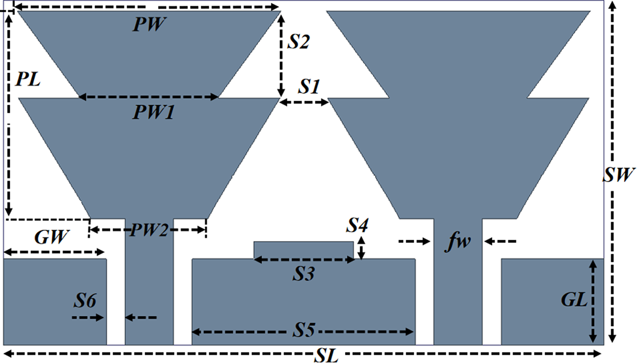
The structural layout and the optimized design specifications of the reported antenna are presented in Fig. 2. At the top, the antenna incorporates a CPW-fed dual-element MIMO architecture, wherein each radiating element is designed with a stepped triangular profile. The radiators are positioned in close proximity with a carefully optimized spatial alignment, yielding a compact and distinctive structural topology. The systematic transformation of the triangular geometries is strategically implemented to enhance key electromagnetic performance metrics, thereby optimizing the overall operational characteristics of the antenna system. The overall antenna structure features a compact form factor measuring 35 × 20 × 1.6 mm3 and has been designed on textile-based jeans substrate (εr = 2.0 and h = 1.6 mm) with the key geometrical parameters (in mm) are, SL = 35, SW = 20, fw = 2.35, S1 = 2.76, S2 = 5.06, S3 = 5.8, S4 = 1, S5 = 13, S6 = 1.08, GW = 6, GL = 5, PW = 15.3, PL = 5.45, PW1 = 8, PW2 = 6.8, fw = 2.84. Figure 3 depicts the evolutionary progression of the proposed antenna architecture, detailing the design refinements at each developmental stage.
Geometrical layout of proposed MIMO antenna.

Figure 2 Long description
and a nearby vertical dimension arrow is labeled S6; a horizontal dimension label PW2 appears near this left lower section. Across the lower central region, a long horizontal dimension arrow labeled S5 runs near the bottom and above it a shorter horizontal dimension arrow labeled S3 spans the central block; a smaller horizontal dimension arrow labeled S4 is placed above S3. On the lower right, a vertical rectangular section is marked with a vertical dimension label GL. The figure shows only symbolic dimension labels and does not display numeric values or units.shows only symbolic dimension labels and does not display numeric values or units.
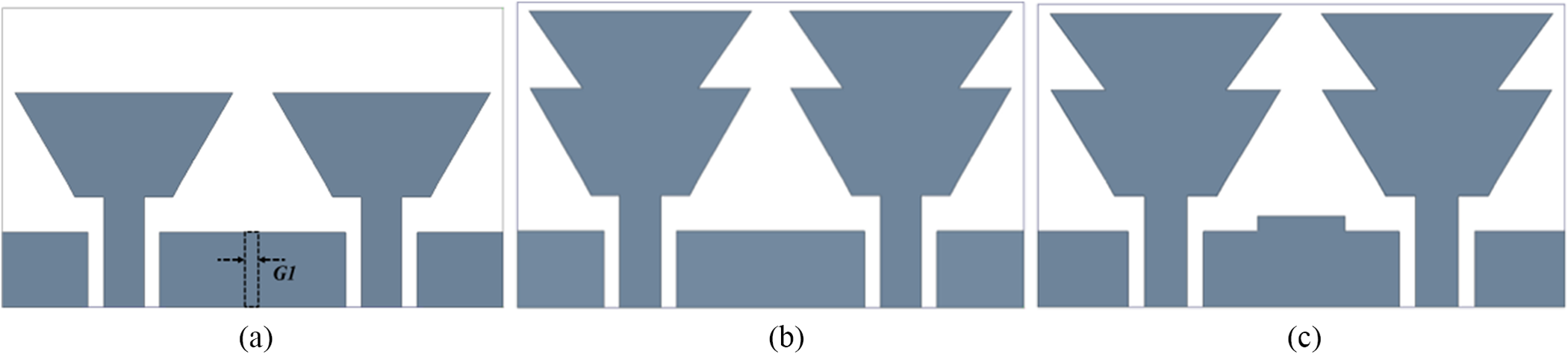
Design iteration and optimization stages of the antenna: (a) Geometry-1, (b) Geometry-2, and (c) Geometry-3.

Figure 3 Long description
The diagram illustrates the design iterations of a coplanar waveguide-fed antenna. In Geometry-1, two triangular radiating elements are positioned side by side, with a central gap labeled 'G1' in the feed region. Geometry-2 shows an enlarged version of the triangular elements, with the gap removed, indicating a change in the feed structure. Geometry-3 maintains the size of the triangular elements but introduces a central rectangular block between the feed sections, suggesting a modification in the ground connection or impedance matching. Each iteration reflects adjustments in the antenna's layout to optimize electromagnetic performance. No dimensions are shown. The diagram serves to illustrate the plan-view geometry and layout changes across the iterations.
The initial configuration, denoted as Geometry-1, incorporates a dual-element layout employing modified triangular-shaped radiators, serving as the baseline structure from which further structural optimization and performance enhancements are derived. The electromagnetic characterization of the proposed structure reveals a dominant resonant mode centered at 4.7 GHz with a 1.1 GHz bandwidth (4.2–5.3 GHz) and a corresponding gain of 2.9 dBi as illustrated in Fig. 4(a)–(c).
Performance evaluation of designed geometries illustrating (a) comparisons of |S11|, (b) inter-element isolation, and (c) comparative gain analysis.

Figure 4 Long description
labeled (a), (b) and (c), each with three line series labeled Geometry-1, Geometry-2 and Geometry-3 (Prop.). (a) The y-axis label is vertical bar S subscript 1 1 vertical bar (decibel). The x-axis label is Frequency (gigahertz). The x-axis runs from 3 to 11. The y-axis runs from 0 to minus 50. Three curves are shown. Geometry-1 has a dip near about 4, rises toward about minus 10 around 6 to 7, then stays between about minus 10 and minus 20 up to 11. Geometry-2 dips near about 4 to about minus 20, rises to around minus 10 near about 6, then stays near about minus 10 to minus 15 up to 11. Geometry-3 (Prop.) dips near about 4 to about minus 25, rises to around minus 10 near about 6, then shows a deeper dip near about 7 to 8 to around minus 35 and returns toward about minus 10 by about 10 to 11. (b) The y-axis label is vertical bar S subscript 2 1 vertical bar (decibel). The x-axis label is Frequency (gigahertz). The x-axis runs from 3 to 11. The y-axis runs from 0 to minus 40. Three curves are shown. Geometry-1 starts near about minus 5 at 3, decreases to around minus 15 near about 5, then trends upward toward about minus 10 by about 7 and continues downward to around minus 20 by about 11. Geometry-2 starts near about minus 5 at 3, stays around minus 10 to minus 15 from about 4 to 7, then drops sharply near about 9 to around minus 35 and rises back toward about minus 15 by about 11. Geometry-3 (Prop.) starts near about minus 5 at 3, stays around minus 10 to minus 15 from about 4 to 8, then drops sharply near about 9 to around minus 30 and rises back toward about minus 15 by about 11. (c) The y-axis label is Total Gain (decibel isotropic). The x-axis label is Frequency (gigahertz). The x-axis runs from 0 to 10. The y-axis runs from 0 to 8. Three curves are shown. Geometry-1 rises from about 1 at 0 to about 3 near about 3, then stays around 2 to 3 up to about 10. Geometry-2 is around 3 to 4 from about 0 to 4, drops sharply near about 5 to near 0, then rises to around 6 to 7 from about 7 to 10. Geometry-3 (Prop.) is around 3 to 4 from about 0 to 4, drops sharply near about 5 to near 0, then rises to around 6 to 7 from about 7 to 10, with a peak near about 8 to 9 around 7.labeled (a), (b) and (c), each with three line series labeled Geometry-1, Geometry-2 and Geometry-3 (Prop.). (a) The y-axis label is vertical bar S subscript 1 1 vertical bar (decibel). The x-axis label is Frequency (gigahertz). The x-axis runs from 3 to 11. The y-axis runs from 0 to minus 50. Three curves are shown. Geometry-1 has a dip near about 4, rises toward about minus 10 around 6 to 7, then stays between about minus 10 and minus 20 up to 11. Geometry-2 dips near about 4 to about minus 20, rises to around minus 10 near about 6, then stays near about minus 10 to minus 15 up to 11. Geometry-3 (Prop.) dips near about 4 to about minus 25, rises to around minus 10 near about 6, then shows a deeper dip near about 7 to 8 to around minus 35 and returns toward about minus 10 by about 10 to 11. (b) The y-axis label is vertical bar S subscript 2 1 vertical bar (decibel). The x-axis label is Frequency (gigahertz). The x-axis runs from 3 to 11. The y-axis runs from 0 to minus 40. Three curves are shown. Geometry-1 starts near about minus 5 at 3, decreases to around minus 15 near about 5, then trends upward toward about minus 10 by about 7 and continues downward to around minus 20 by about 11. Geometry-2 starts near about minus 5 at 3, stays around minus 10 to minus 15 from about 4 to 7, then drops sharply near about 9 to around minus 35 and rises back toward about minus 15 by about 11. Geometry-3 (Prop.) starts near about minus 5 at 3, stays around minus 10 to minus 15 from about 4 to 8, then drops sharply near about 9 to around minus 30 and rises back toward about minus 15 by about 11. (c) The y-axis label is Total Gain (decibel isotropic). The x-axis label is Frequency (gigahertz). The x-axis runs from 0 to 10. The y-axis runs from 0 to 8. Three curves are shown. Geometry-1 rises from about 1 at 0 to about 3 near about 3, then stays around 2 to 3 up to about 10. Geometry-2 is around 3 to 4 from about 0 to 4, drops sharply near about 5 to near 0, then rises to around 6 to 7 from about 7 to 10. Geometry-3 (Prop.) is around 3 to 4 from about 0 to 4, drops sharply near about 5 to near 0, then rises to around 6 to 7 from about 7 to 10, with a peak near about 8 to 9 around 7.
At 4.7 GHz, as illustrated in Fig. 5(a), the surface current initiates at the feed point and propagates along the indicated path toward the upper central region of the patch (shown by the arrows). The total effective path length is approximately 23.75 mm, measured between the two current-minimum points highlighted in red, which corresponds to approximately λ/2 at this frequency. Based on this effective resonant path, the calculated resonance frequency is observed to be 4.5 GHz, obtained using the standard equation [Reference Modak, Kaim, Zaidi, Kanaujia and Rambabu6]. While Geometry-1 demonstrates acceptable performance, the core objective of this work is to achieve ultra-wideband functionality to ensure reliable and high-efficiency 5G communications. Consequently, to accomplish this requirement, Geometry-2 has been systematically developed by integrating an additional modified triangular element into the baseline Geometry-1, resulting in a stepped triangular configuration (see Fig. 3(b)). However, the ground layer remains intact. The intentional geometrical modification alters the effective electrical length of the antenna, thereby extending the surface current path length of 24.8 mm (see Fig. 5(b)). This elongation of the current path reduces the fundamental resonant frequency, shifting it from 4.7 GHz to around 4.16 GHz (within the 3.5–4.6 GHz range). In addition, the incorporated triangular section functions as a parasitic resonant element that electromagnetically couples with the primary radiator, resulting in the excitation of an additional higher-order resonant mode at 8.2 GHz (6.6–9.1 GHz). This mode corresponds to an effective resonant path length of approximately λ/2 (12.77 mm), measured between the two surface current minima indicated by the red arrow in Fig. 5(c). The computed resonant frequencies are observed to be 4.26 and 8.36 GHz, respectively. Despite this, the designed antenna (Geometry-2) provides an enhancement in gains of 3.2 and 6.4 dBi at the respective resonant frequencies. The observed improvement stems from the enlargement of the effective radiating aperture, thereby facilitating a more robust and uniform electromagnetic field distribution across the antenna geometry. Nevertheless, the inclusion of the triangular section also increases electromagnetic coupling between the radiating elements, as evident from the surface current distributions in Fig. 5(c) (marked with a red circle). At 4.1 GHz, a small current concentration is observed along the angular periphery, inducing coupling between the elements and reducing the isolation from 10.1 to 8 dB. Meanwhile, at 8.2 GHz, a stronger inter-element coupling is evident, resulting in an isolation of 16.2 dB.
Distributions of current concentration over antenna structure: (a) Geometry-1@4.7 GHz, (b) Geometry-2@4.1 GHz, (c) Geometry-2@8.2 GHz, (d) Geometry-3@4.7 GHz, and (e) Geometry-3@7.9 GHz.

Figure 5 Long description
The composite figure contains five surface current density vector-field plots labeled (a) through (e), each showing current magnitude in A/m via a color bar and current direction via arrows. There are no x-axis or y-axis labels; spatial information is conveyed entirely through the color bar scale and arrow orientations overlaid on the antenna geometry. Image (a) shows Geometry-1 at 4.7 gigahertz. The color bar ranges from 0.1 to 125 A/m. The highest current concentrations are located at the feedline and at the junction between the feedline and the patch element. Arrows along the feedline point toward the patch and concentration diminishes progressively across the patch surface away from the feed junction. Image (b) shows Geometry-2 at 4.1 gigahertz. The color bar ranges from 0.4 to 97.0 A/m. Compared to image (a), the highest concentrations remain at the feedline and feed junction, but additional concentration is visible along the stepped triangular element edges, indicating current spread into the added triangular section. Image (c) shows Geometry-2 at 8.2 gigahertz. The color bar ranges from 0.4 to 75.2 A/m. At this higher frequency, strong current concentrations appear at the feedline junction and notably along the periphery of the triangular stepped section, with visible hotspots at the notch edges of the stepped feature. Arrow density increases around the triangular element compared to image (b). Image (d) shows Geometry-3 at 4.7 gigahertz. The color bar ranges from 0.3 to 91.6 A/m. The current distribution pattern is similar to image (a) in terms of feedline and junction concentration, but the modified geometry of Geometry-3 produces additional current concentration along the modified element edges not present in Geometry-1. Image (e) shows Geometry-3 at 7.9 gigahertz. The color bar ranges from 0.3 to 96.6 A/m. At this frequency, the hotspots shift from the feedline junction toward the edges and notch regions of the antenna patch, with arrow orientations showing more varied directional patterns across the patch surface compared to image (d) at 4.7 gigahertz.
These observations underscore the inherent trade-off between improved radiation performance and reduced isolation. Moreover, there is a critical requirement to enhance isolation while simultaneously broadening the operational bandwidth for the targeted applications. Concerning this aspect, Geometry-2 is deliberately modified to evolve Geometry-3 by incorporating a parasitic stub connected to the CPW ground plane. The introduced structural refinement enhances isolation and alters the underlying coupling mechanism, thereby enabling a wideband response characterized by distinct resonant peaks at 4.7 and 7.9 GHz, with the overall operational bandwidth extending from 4.0 to 10.2 GHz. However, the gain is significantly reduced to 3.15 dBi. From the surface current distribution illustrated in Fig. 5(d)–(e), it is observed that the introduction of the parasitic stub marginally suppresses the coupling between the antenna elements. This reduction in coupling directly contributes to an improvement in isolation, yielding values of 29.7 dB at 4.7 GHz and 21.2 dB at 7.9 GHz, respectively.
Now, to evaluate the impact of the parasitic stub, a parametric analysis is performed with respect to the design parameter S4 (width of parasitic stub). The results indicate that increasing “S4” progressively shifts the resonant frequency toward the lower band and alters the overall impedance bandwidth, thereby introducing multiband response (see Fig. 6(a)). This behavior is primarily attributed to the increase in the effective electrical length, which lowers the resonant frequency and excites additional resonant modes. Besides, the enhanced surface current interaction between adjacent radiating elements increases the mutual coupling, resulting in degraded inter-element isolation. In addition, the parametric study concerning the length of parasitic stub “S3” has also been carried out, and it was observed that at S3 = 5 mm, the antenna exhibits degraded impedance characteristics due to weak coupling between the parasitic stub and the radiator. As the value increases, the impedance characteristics improve, significantly improving the inter-element isolation to ≈30 and ≈20 dB, respectively, due to effective suppression and redistribution of coupled surface currents by the elongated parasitic stub (see Fig. 6(b)). Notably, at S4 = 1 mm and S3 = 5.8 mm, the antenna exhibits optimized performance, achieving a well-defined resonance with improved impedance bandwidth and enhanced isolation characteristics. Finally, the performance parameters of antenna geometries (Geometry-1, Geometry-2, and Geometry-3) are tabulated in Table 1.
Parametric study in terms of |S11| and |S21| with respect to (a) design parameter S4 and (b) design parameter S3.

Figure 6 Long description
The image showing four line graphs arranged in a two by two layout, with labels (a) between the top and bottom rows and (b) below the bottom row. Top-left graph: The y-axis label is “|S11| (dB)”. The x-axis label is “Frequency (GHz)”. The x-axis shows 4, 6, 8, 10. The y-axis shows 0, minus 10, minus 20, minus 30, minus 40, minus 50. The legend lists: “S4 = 0.5 mm”, “S4 = 1 mm”, “S4 = 2 mm”, “S4 = 3 mm”, “S4 = 4 mm”. Five curves are plotted. The curves start near 0 decibel around 4 gigahertz, drop to minima between about 5 and 6 gigahertz, rise, then show another dip around about 8 gigahertz and rise again toward about minus 10 decibel by about 10 gigahertz. Top-right graph: The y-axis label is “|S21| (dB)”. The x-axis label is “Frequency (GHz)”. The x-axis shows 4, 6, 8, 10. The y-axis shows 0, minus 10, minus 20, minus 30, minus 40, minus 50. The legend lists: “S4 = 0.5 mm”, “S4 = 1 mm”, “S4 = 2 mm”, “S4 = 3 mm”, “S4 = 4 mm”. Five curves are plotted. The curves begin between about minus 5 and minus 15 decibel near 4 gigahertz, dip further between about 5 and 6 gigahertz, then stay around roughly minus 15 to minus 25 decibel through about 8 to 9 gigahertz and show deeper dips near about 10 gigahertz, with one curve reaching close to minus 50 decibel. Bottom-left graph: The y-axis label is “|S11| (dB)”. The x-axis label is “Frequency (GHz)”. The x-axis shows 4, 6, 8, 10. The y-axis shows 0, minus 10, minus 20, minus 30, minus 40, minus 50. The legend lists: “S3 = 5 mm”, “S3 = 5.5 mm”, “S3 = 5.8 mm”, “S3 = 6 mm”, “S3 = 6.5 mm”. Five curves are plotted. The curves start near 0 decibel around 4 gigahertz, show a deep minimum between about 5 and 6 gigahertz for at least one curve reaching near minus 50 decibel, then rise and show another minimum around about 8 gigahertz, with one curve dipping to around minus 40 decibel and then rise toward about minus 10 decibel by about 10 gigahertz. Bottom-right graph: The y-axis label is “|S21| (dB)”. The x-axis label is “Frequency (GHz)”. The x-axis shows 4, 6, 8, 10. The y-axis shows 0, minus 10, minus 20, minus 30, minus 40, minus 50. The legend lists: “S3 = 5 mm”, “S3 = 5.5 mm”, “S3 = 5.8 mm”, “S3 = 6 mm”, “S3 = 6.5 mm”. Five curves are plotted. The curves begin around minus 10 decibel near 4 gigahertz, dip between about 5 and 6 gigahertz with one curve reaching near minus 50 decibel, then rise to around minus 15 to minus 25 decibel through about 7 to 9 gigahertz and show another dip near about 10 gigahertz, with several curves reaching below minus 30 decibel.
Comparative performance analysis across various design stages

Table 1 Long description
The table compares three antenna geometry design stages using geometry type, resonant frequency values, bandwidth, isolation magnitude, and gain. Geometry 1 is a modified triangular design with a resonant frequency of 4.7 GHz, bandwidth of 1.1 GHz, isolation of 10.1 dB, and gain of 2.9 dBi. Geometry 2 is a stepped triangular design with resonant frequencies at 4.16 and 8.2 GHz, bandwidths of 1.1 and 2.5 GHz, isolation values of 8 and 14 dB, and gains of 3.2 and 6.4 dBi. Geometry 3, a stepped triangular design with modified ground, has resonant frequencies at 4.7 and 7.9 GHz, a bandwidth of 6.2 GHz, isolation values of 29.7 and 21.2 dB, and a maximum gain of 3.15 dBi. Overall, Geometry 3 shows the largest bandwidth and the highest isolation compared with the earlier geometries. Geometry 2 provides the highest reported gain value, but its isolation is lower than Geometry 3 and its bandwidth is smaller. Some entries list multiple values per geometry, indicating performance at more than one operating band, so comparisons should be made band by band.
MIMO diversity characterization
This section aimed at measuring the diversity parameters of the suggested antenna arrangement. Beyond conventional antenna properties, an MIMO system requires a more specialized assessment of specific diversity measures to ensure efficient operation and robust system performance. The envelope correlation coefficient (ECC) is a key metric among the various diversity parameters, which measures the response of the MIMO antenna elements to the propagating signals and thus provides a measure of the degree of correlation between the radiating elements.
Ideally, an ECC of zero signifies that the signal paths are uncorrelated and optimal. Further, to evaluate the MIMO performance, the diversity gain (DG) has also been analyzed. Figure 7(a) reveals that the ECC is below the threshold of 0.5, implying low channel correlation, whereas the DG has a value greater than 9.9 within the operating band. Moreover, channel capacity loss (CCL) is also a crucial performance metric, as it aids in measuring the degree to which the performance of the data transmission system is impaired by mutual coupling and correlation of the antenna elements. A reduced CCL represents an improvement in channel utilization and minimum signal deterioration. Another important parameter to elucidate the MIMO antenna performance is the mean effective gain (MEG), which measures the average power received by the antenna compared to an ideal reference antenna in the same propagation conditions. This helps us to understand the efficacy of the antenna in real-world scenarios. As illustrated in Fig. 7(b), the CCL does not exceed 0.3 bits/s/Hz, indicating that the channel performance is not substantially reduced. Likewise, the MEG ratio is maintained below −3 dB as shown in Fig. 7(c). Noteworthy, all the diversity metrics have been calculated using the scattering parameters of each antenna element of the MIMO, with standard formulations determined in papers [Reference Modak and Khan34, Reference Modak, Farooq and Lokam35].
Computed diversity metrics: (a) ECC, (b) CCL, and (c) MEG.

Figure 7 Long description
The image A showing a line graph with two plotted series and the label “(a)” below the plot. The x-axis is labeled “Frequency (GHz)” with tick labels 4, 6, 8 and 10. The left y-axis has tick labels 0.00, 0.01, 0.02 and 0.03. The right y-axis has tick labels 9.995, 9.996, 9.997, 9.998, 9.999 and 10.000. A legend shows “ECC” and “DG”. The ECC series is a black line with circular markers. The DG series is a blue line with square markers. The DG series lies near the top of the plot close to the right-axis value 10.000 across the shown frequency range. The ECC series stays close to 0.00, with a small rise around the mid frequencies and then returning close to 0.00 toward the higher frequencies. The image B showing a single-series line graph with the label “(b)” below the plot. The y-axis is labeled “CCL (Bits/S/Hz)” with tick labels 0.0, 0.3, 0.6 and 0.9. The x-axis is labeled “Frequency (GHz)” with tick labels 4, 6, 8 and 10. A blue line starts near 0.9 at the left side, drops steeply to near 0.0 by around 4 gigahertz, then varies at low values with small rises and dips, ending around 0.2 near the right side. The image C showing a line graph with three plotted series and the label “(c)” below the plot. The x-axis is labeled “Frequency (GHz)” with tick labels 4, 6, 8 and 10. The y-axis is labeled “MEG (dB)” with tick labels 5, 0, minus 5, minus 10 and minus 15. A legend shows “MEG1”, “MEG2” and “MEG1/MEG2”. The MEG1 series is a black line with square markers and stays between about minus 6 and minus 8 across the frequency range. The MEG2 series is a red line with circular markers, starting near minus 13 at the left, rising to around minus 6 near the lower frequencies, then staying between about minus 6 and minus 8 toward the right. The MEG1/MEG2 series is a blue line with triangular markers and stays close to 0 across the frequency range.
Conformability analysis
In wearable electronic platforms, evaluating the antenna’s performance under conformal deformation is essential, as the radiating structure must adapt to diverse body-curvature geometries. Such mechanical bending can alter the antenna’s electromagnetic characteristics, including impedance matching, resonance stability, and radiation behavior; these insights are instrumental in validating the antenna’s suitability for real-time wearable applications. Accordingly, the proposed antenna has been systematically examined under multiple bending radii applied along the X-axis, as illustrated in Fig. 8. The corresponding reflection coefficient and isolation characteristics presented in Fig. 9(a) and (b) demonstrate that the antenna preserves robust and consistent performance under various bending scenarios.
Analysis of conformability on different radii along X-axis: (a) 20 mm, (b) 40 mm, and (c) 60 mm.

Figure 8 Long description
Three sub-images are arranged left to right and labeled (a), (b) and (c). (a) A curved rectangular strip shows a repeating geometric pattern across its surface. A small marker near the lower-left edge is labeled “X”. The label “(a)” appears below, followed by “20 mm”. (b) A similar curved strip with the same repeating geometric pattern. The label “(b)” appears below, followed by “40 mm”. (c) A similar curved strip with the same repeating geometric pattern. The label “(c)” appears below, followed by “60 mm”.
Performance analysis under mechanical deformation: (a) |S11| and (b) |S21|.

Figure 9 Long description
The image shows two line graphs. (a) The graph of magnitude of S subscript 11 in decibels versus frequency in gigahertz. The x-axis is labeled 'Frequency (GHz)' ranging from 4 to 10. The y-axis is labeled '|S11| (dB)' ranging from -60 to 0. Four curves represent different conditions: Rx equals 20 mm (red), Rx equals 40 mm (blue), Rx equals 60 mm (magenta) and flat (black). Resonance dips occur around 4–5 GHz and 8–10 GHz, with the deepest notch near -55 dB for Rx equals 20 mm. (b) The graph of magnitude of S subscript 21 in decibels versus frequency in gigahertz. The x-axis is labeled 'Frequency (GHz)' ranging from 4 to 10. The y-axis is labeled '|S21| (dB)' ranging from -60 to 0. The same four conditions are plotted. Resonance dips are observed around similar frequencies, with the deepest notch near -50 dB for Rx equals 20 mm. The graphs illustrate how bending affects the antenna's performance, with varying resonance depths and frequencies for different Rx values.
Nevertheless, with a reduction in the bending radius, a gradual downward shift of the resonant frequency toward the lower-frequency region is evident. This detuning phenomenon becomes more pronounced at a bending radius of Rx = 20 mm, where severe mechanical deformation induces substantial perturbations in the current distribution and effective electrical length of the radiator, thereby markedly modifying its inherent electromagnetic behavior. Following this, the antenna isolation (|S21|) characteristics are also affected, as evidenced by Fig. 9(b). The isolation response indicates increased mutual coupling in the lower frequency region, with the effect becoming progressively more pronounced as the bending radius decreases. Overall, the analysis demonstrates that mechanical deformation of the antenna structure introduces only marginal perturbations to its electromagnetic behavior, illustrating stable operational characteristics within the operational frequency spectrum.
Safety considerations
Since the antenna is intended for on-body operation, its emitted EM fields can interact with adjacent biological tissues, leading to localized energy absorption and consequent thermal loading. Sustained exposure to this EM radiation may result in a measurable rise in tissue temperature, thereby posing potential health risks [Reference Ashyap, Raad, Tubbal, Khan and Abulgasem36]. The SAR is a dosimetric parameter that quantifies the rate at which EM energy is absorbed by biological tissues. Accordingly, to assess compliance with user safety requirements, an SAR evaluation is performed using a homogeneous body model available in the ANSYS HFSS electromagnetic solver. The electrical property is assigned relative permittivity (Ɛr) and conductivity (σ) values of 50.8 and 3.01 S/m (muscle), at the lower operating frequency of 4.0 GHz. To realistically account for the presence of clothing, an intermediate dielectric spacer of 6 mm thickness with a relative permittivity (Ɛr = 2.0) is inserted between the antenna and the tissue mode [Reference Ali, Ullah, Kamal, Matekovits and Altaf15, Reference Lin, Chen, Gong, Seet, Huang and Lu18].
As shown in Fig. 10(a)–(b), SAR evaluation is carried out at two different resonant frequencies using an initial input power P in = 1 W to estimate the maximum allowable input power in accordance to comply with safety limit. The computed average SAR (ASAR) attains a peak value of 1.12 W/kg at 4.7 GHz, while reduced ASAR levels of 0.89 W/kg are observed at 7.9 GHz, respectively. These elevated ASAR values are within the recommended safety standards established by IEEE and ICNIRP [Reference Ali, Ullah, Kamal, Matekovits and Altaf15, Reference Modak, Lokam and Farooq22, Reference Tiwari, Kaim, Singh, Khan and Kanaujia37, Reference Hazarika, Basu and Kumar38].
Characterization of EM field absorption in human tissues (a) 4.7 GHz and (b) 7.9 GHz.

Figure 10 Long description
The image A showing a spatial heatmap labeled “(a)” below the plot. No row labels, column labels, category labels, or axis labels are shown. A horizontal legend bar is below the heatmap, labeled “W/kg” at the right end. The legend tick labels are “0.1”, “0.64” and “1.12”. The heatmap contains a broad low-intensity background with several higher-intensity patches, including a concentrated hotspot area near the central region of the mapped shape. The image B showing a spatial heatmap labeled “(b)” below the plot. No row labels, column labels, category labels, or axis labels are shown. A horizontal legend bar is below the heatmap, labeled “W/kg” at the right end. The legend tick labels are “0.1”, “0.51” and “0.89”. The heatmap shows a low-intensity background with a smaller number of higher-intensity patches, including a prominent hotspot area near the central region of the mapped shape. In both images, the legend indicates that lower legend values correspond to lower mapped magnitude and higher legend values correspond to higher mapped magnitude.
Measurement set-up and analysis
The effectiveness of the reported multielement antenna design specifically tailored to meet the intended applications has been well tested through comprehensive experimental analyses, with the antenna being manually fabricated on a flexible jeans substrate shown in Fig. 11(a). Each port of the fabricated antenna prototype is equipped with a soldered SMA (F) connector (EMPCB.SMAFSTJ.B.HT) to ensure effective power transmission. Further, to validate the consistency of the simulated solutions, S-parameter measurements are performed via a vector network analyzer (MS46122B), and the respective experimental arrangement is illustrated in Fig. 11(b). The comparison of the simulated and experimentally obtained S-parameters (|S11|) is shown in Fig. 12(a). In a free-space environment, the antenna shows a measured bandwidth of 6.6 GHz (4.1–10.7 GHz), while its response for isolation between the two ports is up to 36.5 dB at 9.9 GHz (see Fig. 12(b)). The practical viability of the proposed antenna is shown methodically by the study of its performance on realistic hand of a human being as depicted in Fig. 11(c).
Fabricated prototype and measurement setups.

Figure 11 Long description
The image consists of three distinct sections labeled a, b and c. In section a, the top and bottom views of a fabricated antenna prototype are shown. Each port of the antenna is equipped with a soldered SMA connector, ensuring effective power transmission. Section b illustrates the free space measurement setup, where the antenna is connected to a vector network analyzer. A computer screen displays the measurement results and the setup is labeled 'Free Space Measurement.' Section c depicts the on-body measurement setup, where the antenna is placed on a person's arm. The environment includes a horn antenna and an antenna under test, labeled 'Horn Antenna' and 'AUT,' respectively. The setup is conducted in an anechoic chamber, which is designed to minimize reflections and external noise during testing.
Performance verification through simulated and measured comparisons (a) |S11|, (b) |S21|, and (c) gain.

Figure 12 Long description
A three part figure labeled (a), (b), (c). The image A showing a line graph labeled (a). The x-axis is labeled Frequency (GHz) with ticks at 4, 6, 8, 10. The y-axis is labeled magnitude of S subscript 11 (dB) with ticks at 0, minus 10, minus 20, minus 30, minus 40, minus 50. A legend shows Free Space with Sim. and Mea. and On-Body with Sim. and Mea. Four curves are plotted. The Free Space Sim. curve drops from near 0 decibel around 4 gigahertz to a deep minimum near minus 50 decibel around about 5 gigahertz, then rises toward about minus 10 decibel by about 10 gigahertz. The Free Space Mea. curve follows a similar shape with a minimum around the 5 to 6 gigahertz region and values mostly between about minus 10 and minus 30 decibel from about 6 to 10 gigahertz. The On-Body Sim. and On-Body Mea. curves show shallower minima than the Free Space Sim. curve, with dips in the mid band and values generally between about minus 10 and minus 30 decibel across most of 4 to 10 gigahertz. The image B showing a line graph labeled (b). The x-axis is labeled Frequency (GHz) with ticks at 4, 6, 8, 10. The y-axis is labeled magnitude of S subscript 21 (dB) with ticks at 0, minus 10, minus 20, minus 30, minus 40, minus 50. A legend shows Free Space with Sim. and Mea. and On-Body with Sim. and Mea. Four curves are plotted. The curves start near about minus 10 decibel around 4 gigahertz, dip further in the 5 to 7 gigahertz region and then trend downward again toward higher frequency. One measured curve reaches a low near about minus 50 decibel close to 10 gigahertz, while other curves are higher, around the minus 20 to minus 40 decibel range near 10 gigahertz. The image C showing a line graph labeled (c). The x-axis is labeled Frequency (GHz) with ticks at 4, 6, 8, 10. The y-axis is labeled Total Gain (dBi) with ticks at 0, 1, 2, 3, 4. A legend shows Sim. and Mea. Two curves are plotted. The simulated curve rises from about 1 decibel isotropic around 4 gigahertz to around 2 decibel isotropic near 6 gigahertz, reaches a peak near about 3 to 4 decibel isotropic around 8 to 9 gigahertz, then decreases toward about 2 decibel isotropic by about 10 gigahertz. The measured curve stays lower, around about 0.5 to 2 decibel isotropic, with a dip around the mid band and a smaller rise near about 8 to 9 gigahertz.
Figure 12(a) shows the simulated and measured |S11| comparison for on-body configuration, which shows a slight downward shift in the resonant frequency, results in offering a wide operational bandwidth of 6.8 GHz (3.3–10.1 GHz), compared to the simulated counterparts, with corresponding maximum isolation levels of 29.1 dB, respectively. This analysis provides a comparable performance between the simulated and measured results, with only minor discrepancies observed in the resonant frequencies and impedance bandwidths, which are unavoidable. This behavior is primarily due to manual fabrication limitations, including inaccuracies in cutting conductive textile, manual alignment of the radiating elements, connector soldering inaccuracies, and non-uniform adhesive bonding between the conductive layer and textile substrate. Additionally, textile substrates inherently exhibit variations in dielectric properties, thickness, and surface roughness, while also being highly sensitive to mechanical deformation. Further, the antenna attains a maximum measured gain of 3.3 dBi@9.0 GHz, making it highly fit for indoor environmental applications (see Fig. 12(c)). Figure 13(a) and (b) shows the simulated 3D far-field radiation patterns of the antenna along with 2D (simulated and measured) in both the planes of φ = 0° and φ = 90° (see Fig. 13(c) and (d)) at two different resonant frequencies within the operating band. At 4.7 GHz, the antenna exhibits quasi-directional radiation pattern with a dominant main lobe and minor side lobes, while at 7.9 GHz, a directional radiation pattern with the main beam tilted by approximately 25°–30° from the boresight direction. Moreover, in both planes, the measured result shows a noticeable distortion, primarily due to several electromagnetic effects during measurements.
2D and 3D far-field radiation patterns.

Figure 13 Long description
The image A showing a pair of 3D far-field radiation patterns. The left pattern is at a frequency of 4.7 GHz and the right pattern is at a frequency of 7.9 GHz. Both patterns use a spherical coordinate system with Theta in degrees along the vertical axis and Phi in degrees along the horizontal axis. The 3D surfaces show the spatial distribution of the radiated field across all angular directions. The image B showing four 2D polar radiation pattern plots arranged in two columns. The left column corresponds to 4.7 GHz and the right column corresponds to 7.9 GHz. In the 4.7 GHz polar plot, the angular axis spans 0 to 360 degrees in increments of 60 degrees, labeled at 0, 60, 120, 180, 240 and 300 degrees. The radial axis is labeled in decibels and spans from 0 at the outermost ring inward to minus 12 decibels, with intermediate rings at minus 4 and minus 8 decibels. Four curves are plotted. The simulated E-plane curve is marked with filled circles. The simulated H-plane curve is marked with filled squares. The measured E-plane curve is marked with filled triangles pointing upward. The measured H-plane curve is marked with filled triangles pointing downward. At 4.7 GHz, the simulated E-plane and H-plane curves show a broad main lobe centered near 0 degrees with relatively smooth sidelobe structure. The measured E-plane and H-plane curves follow the simulated patterns closely near the main lobe but show visible deviations in the sidelobe regions, particularly between 120 and 240 degrees, where the measured curves dip to approximately minus 10 to minus 12 decibels. In the 7.9 GHz polar plot, the angular axis uses the same 0 to 360 degree range and radial scale from 0 to minus 12 decibels. The same four curve types appear: simulated E-plane with filled circles, simulated H-plane with filled squares, measured E-plane with filled triangles pointing upward and measured H-plane with filled triangles pointing downward. At 7.9 GHz, the main lobe of the simulated E-plane curve is tilted from the 0 degree boresight direction by approximately 25 to 30 degrees. The simulated H-plane shows a broader beam shape. The measured E-plane and H-plane curves exhibit greater distortion relative to the simulated curves compared to the 4.7 GHz case, with irregular sidelobe levels visible between 90 and 270 degrees, reaching levels between minus 8 and minus 12 decibels.
Conclusion
An MIMO antenna system with dual elements has been successfully developed and experimentally validated through detailed measurements. The antenna designs are formed by a stepped triangular profile, and each antenna is evanescently aligned with a well-optimized space geometry, yielding a compact and unique structural topology with an improved electromagnetic performance of 4.0–10.2 GHz spanning the entire UWB spectrum. Besides, it provides a gain of 3.15 dBi with a minimum isolation of 21.2 dB. The MIMO diversity properties and the applicability in body-worn are further investigated using conformal analysis and safety measurements. Overall, the experimental findings are consistent with the simulated counterparts across all electromagnetic performance parameters. This validates the applicability of the proposed antenna for wearable 5G communication. A key performance parameter comparison in relation to prior art is reported in Table 2.
Comparison of key performance parameters in relation to prior art

Table 2 Long description
The table compares eight multiport antenna designs by geometry, substrate, number of ports, physical size, operating frequency bands, bandwidth, gain, isolation, flexibility, SAR reporting, diversity metrics, and intended application. The proposed work uses a stepped triangular geometry with a modified ground on a jeans substrate, has 2 ports, measures 35 by 20 by 1.6 millimeters, operates from 4.0 to 10.2 gigahertz, and has 6.2 gigahertz bandwidth with gain 3.15 dBi. Its isolation is reported as a minimum of 21.2 dB and its envelope correlation coefficient is 0.002, among the lowest values in the table, with diversity gain 9.99 and channel capacity loss 0.25. The widest bandwidth overall is in reference 30, a 4‑port circular ring design spanning 2.8 to 14.2 gigahertz with 11.4 gigahertz bandwidth, but it is not bendable and does not report SAR. The highest gains appear in reference 26 at 8.3 and 13.0 dBi across two bands, but its bandwidths are relatively narrow at 0.4 and 0.95 gigahertz. Several wearable entries use textile-like substrates such as jeans, felt, or polyimide and often report bending and SAR, while some rigid-substrate entries do not. Isolation values vary widely, from 12 dB in reference 25 up to 47 dB in reference 30, and ECC ranges from 0.001 to 0.16, so comparisons should consider that some rows list multiple bands and some metrics are missing or reported differently across studies.
BW = bandwidth; CP = circular polarization; NA = not available.
Acknowledgements
The authors are thankful to CRIF NIT Warangal for providing the necessary facilities for conducting the experiments.
Funding statement
No funding is available.
Competing interests
The authors report no conflict of interest.

Alekhya B is currently pursuing her Ph.D. in the Department of Electronics and Communication Engineering, National Institute of Technology Warangal, Telangana, India. She is also associated with the Department of Electronics and Communication Engineering, VNR Vignana Jyothi Institute of Technology, Hyderabad, Telangana, India. Her current research interests include wearable antennas for 5G communications.

Lokam Anjaneyulu obtained his B.Tech. (ECE) in 1989, M.Tech. from R.E.C (N.I.T), Warangal in 1991, and Ph.D. from N.I.T, Warangal, in 2009. He worked as a Project Officer at the Institute of Armament Technology (DRDO), Pune, India, for 5 years from 1991 and was involved in the design of surface-borne and airborne radar systems for clutter-measurement application. Later, he worked as a Staff Scientist at Helios Systems, Madras, India, for 2 years from 1995 and engaged in the development of radio-wave propagation assessment software modules for ship-borne radars of Indian Navy. He has been with the Department of Electronics and Communications Engineering at National Institute of Technology, Warangal, India, since 1997 and has 25 years of teaching experience. He is presently working as Professor in the department. He has completed few defense R&D Projects from DRDO and ISRO and has around 100 papers to his credit in National and International Conferences and journals. He is a senior member of IEEE, IEEE-APS, Life member of ISTE, Fellow of Institute of Engineers, and Fellow of IETE.

Sumon Modak is currently working as an Assistant Professor at Dr B.R. Ambedkar National Institute of Technology Jalandhar, Punjab, India. He received his Ph.D. degree in Electronics and Communication Engineering from the National Institute of Technology Silchar, Assam, India. His current research interests include UWB and millimeter-wave antennas, EBG structures, CMA, and implantable/ingestible antennas for biomedical applications.