1 Introduction
In the vast literature on wave–mean and wave–vortex interactions, there is a tradition of thinking in terms of wave-induced mean forces and the associated wave-induced momentum fluxes or radiation stresses. The tradition goes back many years, to the work of Lord Rayleigh, Léon Brillouin and other great physicists. It continues today in, for instance, work on the fluid dynamics of atmospheres and oceans, as well as on quantum vortices where the wave-induced mean forces are called ‘Iordanskii forces’.
Within the atmosphere–ocean community, the force-oriented viewpoint is important because wave-induced mean forces are recognized as key to solving what used to be three great enigmas – three grand challenges – in atmospheric science. They were to understand the quasi-biennial oscillation of the zonal winds in the equatorial stratosphere, the ‘antifrictional’ self-sharpening of jet streams, and the gyroscopic or Coriolis pumping of global-scale mean circulations in the stratosphere and mesosphere (i.e. between altitudes
 ${\sim}10{-}100~\text{km}$
) and the consequent water vapour, ozone and pollutant transport and, most dramatically, the refrigeration of the summer mesopause – down to temperatures
 ${\sim}100\,^{\circ }\text{C}$
below radiatively determined temperatures. The history is tortuous and goes back to the 1960s, when all three phenomena were observationally conspicuous but, in terms of mechanism, completely mysterious. See for instance Wallace & Holton (Reference Wallace and Holton1968), Fritts (Reference Fritts1984), Holton et al. (Reference Holton, Haynes, McIntyre, Douglass, Rood and Pfister1995), Baldwin et al. (Reference Baldwin, Gray, Dunkerton, Hamilton, Haynes, Randel, Holton, Alexander, Hirota and Horinouchi2001), Dritschel & McIntyre (Reference Dritschel and McIntyre2008) and Garcia et al. (Reference Garcia, Smith, Kinnison, de la Cámara and Murphy2017).
Recognition of wave-induced mean forces as key to solving all three enigmas, and as essential components of weather and climate models, constituted a gradual, but major, paradigm shift regarding the nature of large-scale momentum transport in atmospheres and oceans. Before the 1960s, such transport tended to be thought of in terms of turbulent eddy viscosities, missing the point that wave-induced momentum transport can be a long-range process more likely to dominate, as in fact it does, over large scales limited not by parcel displacements and mixing lengths but instead by the far greater distances over which waves can propagate.
Much of the atmosphere–ocean literature, especially where it deals with mean forces induced by gravity waves, often takes for granted that the forces can be computed from linearized wave theory alone using what is now called the pseudomomentum rule (e.g. Bühler (Reference Bühler2014), hereafter Reference BühlerB14). That is the accepted basis of gravity-wave ‘parametrization schemes’ in weather and climate models, designed to incorporate the mean forces coming from gravity waves whose wavelengths are too small to be resolved explicitly. It is also the usual basis on which, for instance, Iordanskii forces are computed (e.g. Sonin Reference Sonin1997; Stone Reference Stone2000a ). Pseudomomentum, also called quasimomentum or wave momentum, or phonon momentum, is the linear-theoretic wave property whose non-dissipative conservation depends, through Noether’s theorem, on translational invariance of the mean or background state on which the waves propagate, as distinct from translational invariance of the entire physical system, background plus waves, which implies conservation of momentum.
In a linearized ray-theoretic description the pseudomomentum
 $\unicode[STIX]{x1D5FD}$
per unit mass is
 ${\mathcal{A}}\boldsymbol{k}$
, where
 $\boldsymbol{k}$
is the wavenumber vector and
 ${\mathcal{A}}$
the wave-action, i.e. wave-energy divided by intrinsic frequency, per unit mass (e.g. Bretherton & Garrett Reference Bretherton and Garrett1968). The wave-action, wave-energy and pseudomomentum are linear-theoretic wave properties and are
 $O(a^{2})$
in magnitude, where
 $a$
measures wave amplitude (and will be defined in such a way that
 $a\ll 1$
validates linearization). The pseudomomentum rule says that
 $O(a^{2})$
wave-induced mean forces can be calculated as if pseudomomentum were momentum and the fluid medium were absent.
As discussed for instance in Reference BühlerB14, the rule has been justified mainly for simplified mean flows that are themselves translationally invariant. In such cases it is typical, as is well known, for persistent mean forces with cumulative effects to arise only when the waves break or are otherwise dissipated, leading to a persistent pseudomomentum-flux convergence. However, when the waves are refracted by realistic, three-dimensional backgrounds involving vortices, the situation is fundamentally different. One can get persistent mean forces with cumulative effects in the absence of wave dissipation. Also, it is unclear whether, or when, or in what sense the pseudomomentum rule should hold. The fluid medium is not absent, and it supports a mean pressure field that mediates long-range mean forces of the same order,
 $O(a^{2})$
, as those computed from the pseudomomentum rule. Such pressure fields are not wave properties and cannot be computed from linearized wave theory alone. Rather, they require the solution of equations governing the mean or background state correct to
 $O(a^{2})$
. Cases in which the rule fails for this reason have long been known, going back as far as Brillouin’s pioneering work on acoustic radiation stress (e.g. Brillouin Reference Brillouin1936; Reference BühlerB14 § 12.2.2).
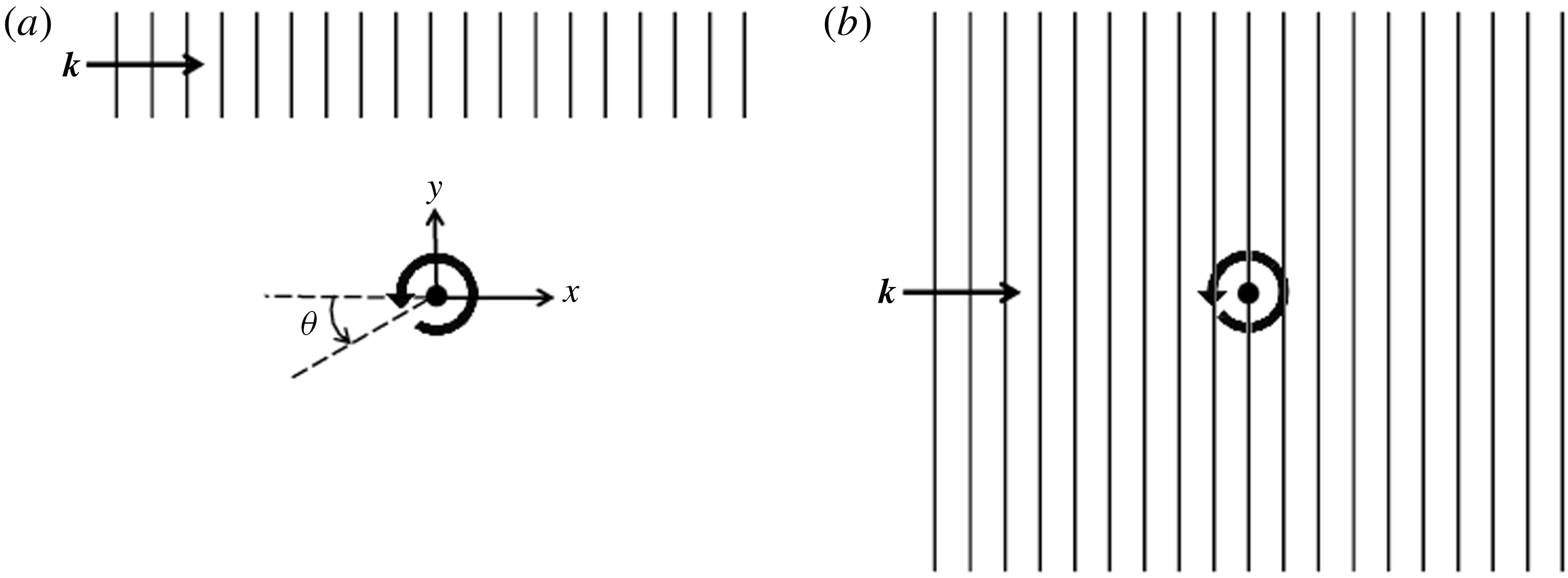
Panels (a) and (b) are schematics of wave–vortex interaction problems (i) and (ii), respectively. Waves of wavenumber
 $\boldsymbol{k}$
are incident from the left and are weakly refracted by the vortex. Rays are nearly parallel to the
 $x$
axis. The azimuthal angle
 $\unicode[STIX]{x1D703}$
is defined unconventionally but in a way that will be convenient when discussing the Aharonov–Bohm effect.

For gravity-wave parametrization, in particular, there are therefore unresolved questions as to how to compute, and indeed how to think about, the wave-induced mean forces for realistic, three-dimensional backgrounds. Current parametrization schemes ignore these questions because they altogether neglect horizontal refraction, giving rise to what is sometimes called the ‘missing forces’ problem for such schemes.
The simplest wave–vortex problems in which these questions arise are to be found in a two-dimensional, non-rotating shallow-water or acoustical setting, with no viscous or other wave dissipation. Two basic examples, the main examples to be studied in this paper, are sketched in figures 1(a) and 1(b). They will be referred to as problem (i) and problem (ii), respectively. The background flow is a single vortex whose vorticity is confined to a core of radius
 $r=r_{0}$
, say, with irrotational flow outside. The coordinates are as shown in figure 1(a), with
 $r^{2}=x^{2}+y^{2}$
. The vortex weakly refracts a train of gravity waves or sound waves incident from the left. The refraction induces a small difference between incoming and outgoing pseudomomentum fluxes – corresponding to the background not being translationally invariant – and the pseudomomentum rule leads us to expect a persistent
 $O(a^{2})$
mean recoil force to be exerted. That expectation is independent of whether or not the waves overlap the vortex core. One reason for studying the two problems side by side is a desire to understand how overlap or non-overlap affect the way in which the recoil force arises, and where it is exerted, as well as whether it complies with the pseudomomentum rule.
Problem (i), with no overlap, has already been studied in an earlier paper (Bühler & McIntyre (Reference Bühler and McIntyre2003), hereafter Reference Bühler and McIntyreBM03) but will be revisited here in order to compare it with problem (ii), for which new results will be obtained. Also new will be results for a rapidly-rotating version of problem (i), to be defined below and to be referred to as problem (iii).
Implicit here, as above, is the assumption that the waves can be described by linearized theory for
 $a\ll 1$
on a background flow of much greater magnitude. Our aim is to obtain precise results by analytical means, in order to gain insight into the questions just noted. To get analytically tractable, precisely soluble problems it turns out that we must also assume, as was done in Reference Bühler and McIntyreBM03, that the background flow and the resulting refraction are very weak in the sense that the vortex must be assumed to have small Froude or Mach number
 $$\begin{eqnarray}\unicode[STIX]{x1D716}=U/c_{0}\ll 1,\end{eqnarray}$$
where
 $U$
is a vortex flow speed and
 $c_{0}$
an intrinsic wave speed. Thus the analyses to be presented fall within the asymptotic regime
 $a\ll \unicode[STIX]{x1D716}\ll 1$
. For definiteness,
 $U$
will be taken to be the flow speed at the edge
 $r=r_{0}$
of the vortex core, and
 $c_{0}$
the wave speed far from the core. For general
 $r\geqslant r_{0}$
the wave speed
 $c=c(r)=c_{0}\{1+O(\unicode[STIX]{x1D716}^{2}r_{0}^{2}/r^{2})\}$
, from the Bernoulli effect and the
 $r^{-1}$
dependence of the vortex flow speed.
The regime
 $a\ll \unicode[STIX]{x1D716}\ll 1$
also encompasses the celebrated Lighthill theory of spontaneous sound emission from, and scattering by, unsteady systems of vortices. It can be contrasted with, for instance, the regime
 $a\sim \unicode[STIX]{x1D716}\ll 1$
(e.g. Lelong & Riley Reference Lelong and Riley1991; Ward & Dewar Reference Ward and Dewar2010; Thomas Reference Thomas2017), in which wave–vortex interactions of the resonant-triad type are possible. The vortical field, if sufficiently complex spatially, can then act as a passive ‘catalyst’ of wave–wave energy transfer very like the Bragg scattering or ‘elastic scattering’ studied in McComas & Bretherton (Reference McComas and Bretherton1977), in a somewhat different context. Yet another regime of interest, one that has been studied very often in past decades, is
 $a^{2}\sim \unicode[STIX]{x1D716}\ll 1$
, for instance in connection with the generation of Langmuir vortices by the non-dissipative Craik–Leibovich instability (e.g. Craik & Leibovich Reference Craik and Leibovich1976; Leibovich Reference Leibovich1980; Reference BühlerB14 § 11.3). Indeed the regime
 $a^{2}\sim \unicode[STIX]{x1D716}\ll 1$
arises naturally in a great variety of problems where mean flows are generated non-dissipatively, from rest, entirely through the presence of waves. Then refraction of the waves by the mean flow comes in only at higher order. Further such examples include, among many others, those studied by Longuet-Higgins & Stewart (Reference Longuet-Higgins and Stewart1964), Bretherton (Reference Bretherton1969), McIntyre (Reference McIntyre1981, Reference McIntyre1988), Wagner & Young (Reference Wagner and Young2015), Haney & Young (Reference Haney and Young2017), Thomas, Bühler & Smith (Reference Thomas, Bühler and Smith2018) and Thomas & Yamada (Reference Thomas and Yamada2019).
Returning now to problems (i)–(iii), in which
 $a\ll \unicode[STIX]{x1D716}\ll 1$
and refraction takes place at leading order in
 $\unicode[STIX]{x1D716}$
, it will be shown in this paper that the pseudomomentum rule is satisfied not only in problem (i) but also in the other two problems, to leading order at least. In all three problems, the background feels a persistent
 $O(a^{2}\unicode[STIX]{x1D716}^{1})$
mean recoil force satisfying the rule.
Problem (ii) is a classical version of the phonon–vortex problem studied in the quantum vortex literature. This classical version is considered for instance by Sonin (Reference Sonin1997) and Stone (Reference Stone2000a
), who take the wavetrain to be infinitely wide, and incident from
 $x=-\infty$
. They argue not only that the pseudomomentum rule holds but also that there is a remarkable simplification, namely that the dominant wave-refraction effect, the sole effect that comes in at leading order,
 $O(a^{2}\unicode[STIX]{x1D716}^{1})$
, is the topological phase jump arising from what is called Aharonov–Bohm effect. We will find, however – with cross-checks from two independent methods – that another, quite different refraction effect is also relevant in problem (ii), except in one special limiting case where the Aharonov–Bohm phase jump is indeed dominant. In that special case the length of the wavetrain is taken to infinity first, followed by the width. If the order of limits is reversed, a different answer is obtained and the Aharonov–Bohm phase jump, while still relevant, is no longer the only relevant refraction effect. However, as already emphasized we find that the pseudomomentum rule is still satisfied to leading order, that is, correct to
 $O(a^{2}\unicode[STIX]{x1D716}^{1})$
.
The Aharonov–Bohm phase jump is a topological property of the wave field most simply expressed via the following far-field solution to the linearized equations. The solution is well known in the quantum literature and will be verified below, in § 2 and appendix A. For sufficiently large
 $r$
, and outside a relatively narrow ‘wake’ region surrounding the positive
 $x$
axis, the wave field has the asymptotic form
 $A\exp (\text{i}\unicode[STIX]{x1D6F7})$
where the amplitude
 $A=$
 $O(a)$
is a real constant, with error
 $O(a\unicode[STIX]{x1D716}^{2}r_{0}^{2}/r^{2})$
, and the phase
 $\unicode[STIX]{x1D6F7}$
is given by
 $$\begin{eqnarray}\unicode[STIX]{x1D6F7}=k_{0}(x-c_{0}t)-\unicode[STIX]{x1D6FC}\unicode[STIX]{x1D703}+\text{const.}\,+\,O(\unicode[STIX]{x1D716}^{2}r_{0}^{2}/r^{2}).\end{eqnarray}$$
The incident wavenumber
 $k_{0}$
is a constant. The azimuthal angle
 $\unicode[STIX]{x1D703}$
is defined as in figure 1(a) and ranges from
 $-\unicode[STIX]{x1D70B}$
to
 $\unicode[STIX]{x1D70B}$
, while
 $\unicode[STIX]{x1D6FC}$
is a constant defined by
 $$\begin{eqnarray}\unicode[STIX]{x1D6FC}=\unicode[STIX]{x1D6E4}k_{0}/2\unicode[STIX]{x1D70B}c_{0}=Uk_{0}r_{0}/c_{0}=k_{0}r_{0}\unicode[STIX]{x1D716},\end{eqnarray}$$
where
 $\unicode[STIX]{x1D6E4}$
is the Kelvin circulation of the vortex. The phase jump
 $2\unicode[STIX]{x1D70B}\unicode[STIX]{x1D6FC}$
across the positive
 $x$
axis is the Aharonov–Bohm phase jump, a topological defect of (1.2). In a full solution it is smoothed out across the wake region. It measures the effect of the vortex flow in compressing the wavetrain on the positive-
 $y$
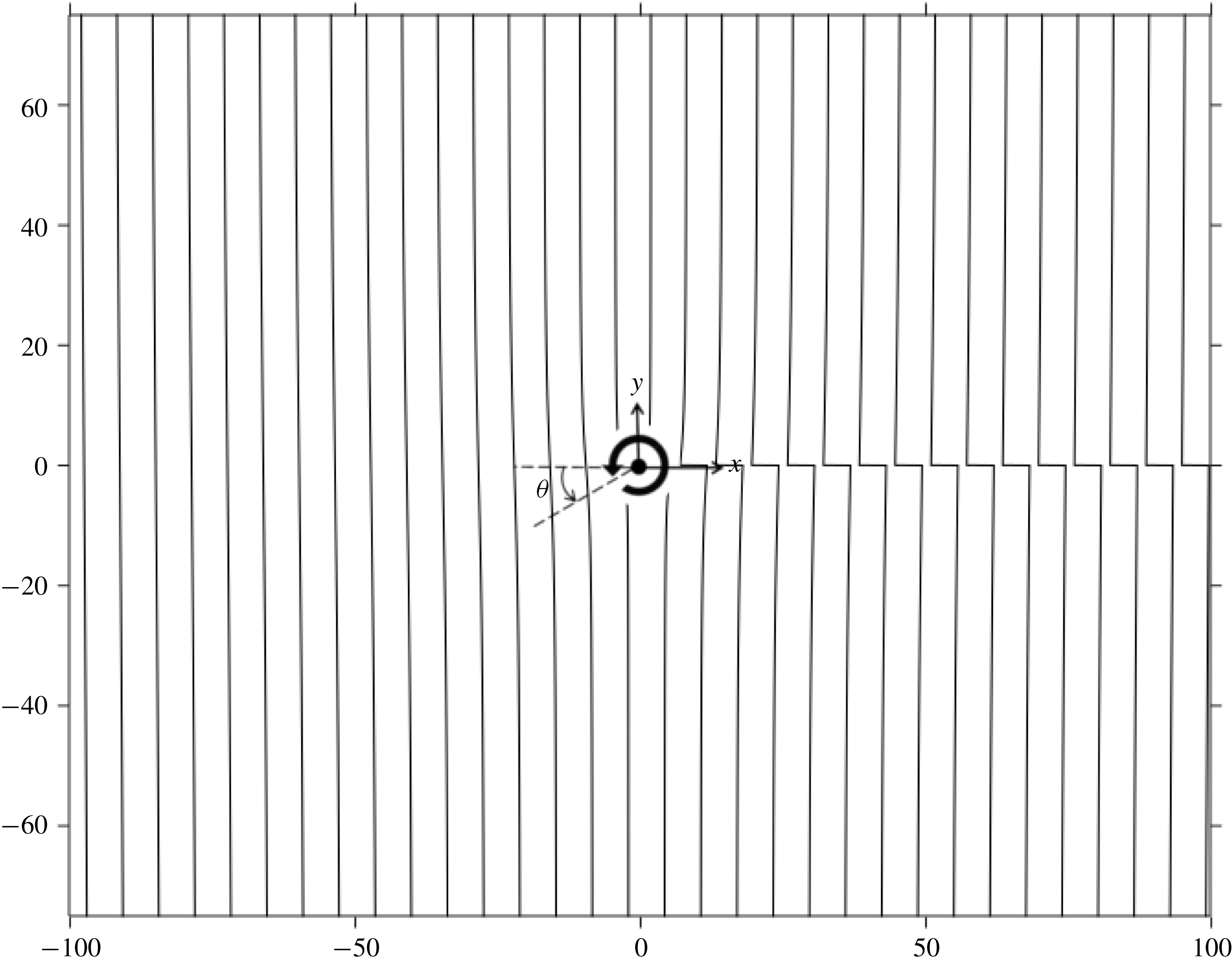
side and stretching it on the negative. The wavecrest shapes
 $\unicode[STIX]{x1D6F7}=$
const. described by (1.2), with the error term neglected, are plotted in figure 2 for
 $\unicode[STIX]{x1D6FC}=0.75$
, fixing the phase jump at three-quarters of a wavelength. Depending on the value of
 $k_{0}r_{0}$
this can take us outside the range of validity of our asymptotic regime (see for instance § 7), but
 $\unicode[STIX]{x1D6FC}=0.75$
is chosen here to make the refraction effects visible in the figure. They include the other relevant effect already mentioned, which is that, except on the
 $y$
axis, the wavecrests are slightly rotated away from the
 $y$
direction, by
 $O(\unicode[STIX]{x1D716}r_{0}/r)$
. This latter effect is also important in problem (i), as noted in Reference Bühler and McIntyreBM03 and in Reference BühlerB14 § 14.2.
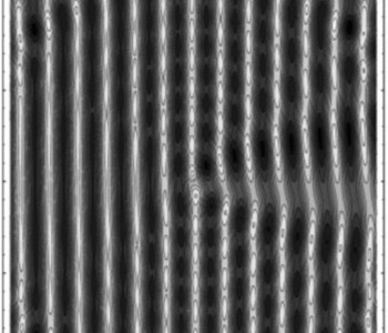
Wavecrests plotted from the far-field solution (1.2), with
 $\unicode[STIX]{x1D6FC}=0.75$
. The unit of length is taken as
 $k_{0}^{-1}$
so that the unrefracted wavelength is
 $2\unicode[STIX]{x1D70B}$
. The Aharonov–Bohm phase jump appears as a phase discontinuity on the positive
 $x$
-axis. In a full solution this discontinuity is smoothed out across a relatively narrow ‘wake’ region.

There remains the question of where the wave-induced recoil force is exerted. The question is ambiguous as it stands, and can be answered in more than one way, but there is one and only one way that avoids bringing in the
 $O(a^{2})$
mean pressure field. It has the further advantage of being the only way that is relevant to gravity-wave parametrization. It is to ask, then answer, the question thus: If the waves were removed and the recoil force exerted artificially, as an external applied force, where should it be exerted in order to have the same effect on the mean flow? As shown in Reference Bühler and McIntyreBM03 and Reference BühlerB14 § 14.2, in the case of problem (i), the answer is not at locations where the waves are refracted – as a naive invocation of the pseudomomentum rule might suggest – but, rather, solely at the location of the vortex core. Reference Bühler and McIntyreBM03 therefore called the recoil ‘remote’. In problem (i), the vortex core can be arbitrarily distant from locations where the waves are refracted. There is of course nothing mysterious about this remoteness – no violation of Newton’s Third Law – because pressure fields can mediate actions and reactions continuously, over substantial distances, just as they do in ordinary vortex–vortex interactions.
To arrive at this picture Reference Bühler and McIntyreBM03 relied mainly on a thought-experiment in which an artificial ‘holding force’ was applied to the vortex core, in such a way as to cancel the recoil due to the waves. It was shown by careful analysis that, by applying this holding force, the mean flow and wave field can be kept exactly steady, with exactly constant total momentum. Here, following Reference BühlerB14 § 14.2, we ask instead how the mean flow responds to the net pseudomomentum flux in the absence of a holding force. The answer is then that the vortex translates, and keeps on translating persistently, in a direction perpendicular to the recoil force – a classic Magnus-force-like scenario. It translates because it is advected by an
 $O(a^{2})$
‘Bretherton flow’ induced by the wave field (Bretherton Reference Bretherton1969). With no holding force, therefore, the Kelvin impulse of the vortex (e.g. Batchelor (Reference Batchelor1967) equation (7.3.7), and equation (3.3) below) changes in just the same way as if the waves were removed and the recoil force artificially applied to the vortex core. Because
 $a^{2}\ll a\ll \unicode[STIX]{x1D716}$
, the wave field can still be treated as steady. And in each problem studied here and in Reference Bühler and McIntyreBM03, the Bretherton flow organizes itself such that the rate of change of impulse corresponds to a recoil force that is consistent with the pseudomomentum rule.
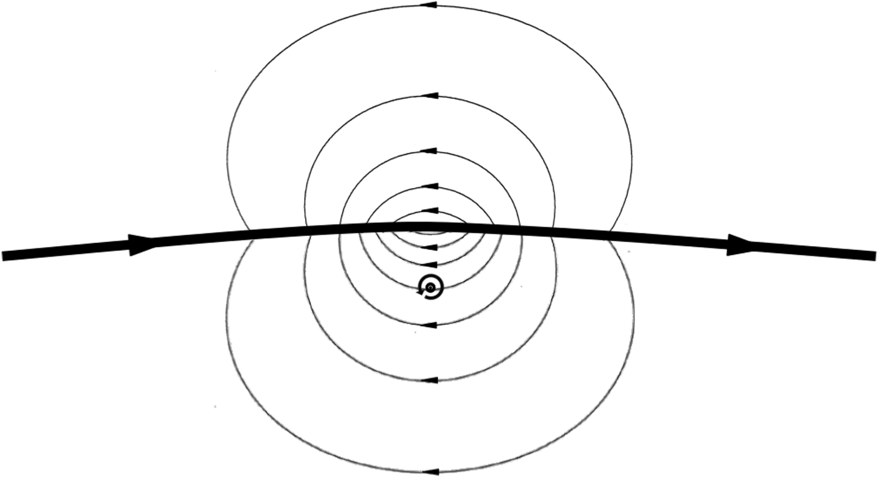
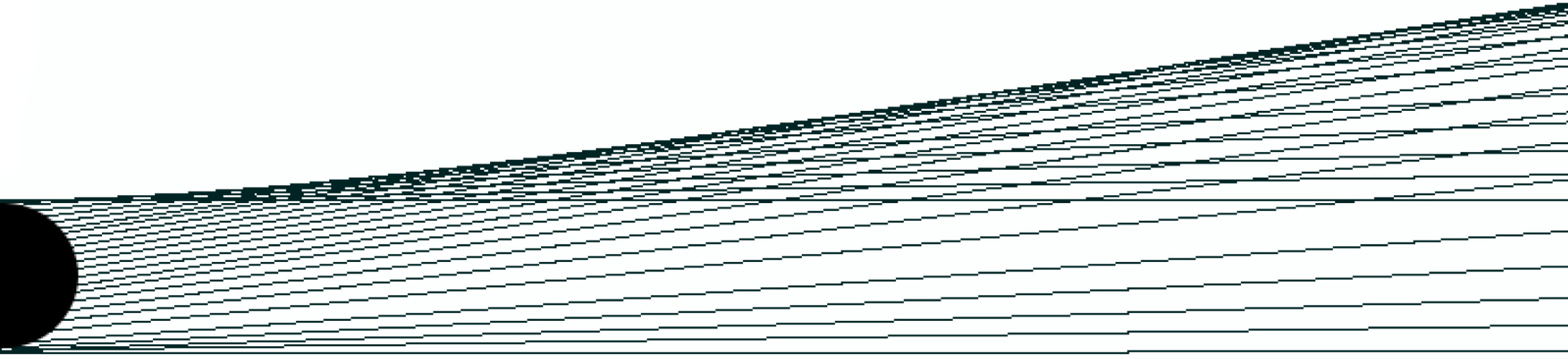
Schematic of the Bretherton flow arising in a version of problem (i) studied in Reference Bühler and McIntyreBM03. The
 $O(a^{2})$
mean flow within a narrow wavetrain, whose ray path is shown by the heavy curve, is dominated by the Stokes drift. A small portion of its mass flux,
 $O(a^{2}\unicode[STIX]{x1D716}^{1})$
in this case, leaks sideways as a consequence of wave refraction. To describe this situation the refraction problem must be considered correct to two orders in
 $\unicode[STIX]{x1D716}$
, as was done in § 5.1 of Reference Bühler and McIntyreBM03. Refraction effects enter at both orders, not only the
 $O(\unicode[STIX]{x1D716})$
effects illustrated in figure 2 but also an
 $O(\unicode[STIX]{x1D716}^{2})$
change in the direction of the absolute group velocity, exaggerated in this schematic.

By way of illustration, figure 3 depicts schematically the Bretherton flow in a version of problem (i) solved in § 5.1 of Reference Bühler and McIntyreBM03, q.v. for the analytical details. The heavy curve represents a narrow wavetrain that is slightly deflected as it goes past the vortex, in such a way that the net pseudomomentum flux into the region points in the positive
 $y$
direction. Ray theory is used to describe the waves, as throughout Reference Bühler and McIntyreBM03, assuming
 $k_{0}r_{0}\gg 1$
. The
 $O(a^{2})$
mean flow within the wavetrain is dominated by the Stokes drift. A small portion of its mass flux leaks sideways as a consequence of wave refraction, forming the Bretherton flow, which is irrotational outside the wavetrain. In the example shown it advects the vortex core leftward, in the negative
 $x$
direction. The corresponding recoil force – a force that would move the vortex core leftward in the absence of waves – is therefore a force in the positive
 $y$
direction, like the net pseudomomentum flux. Its magnitude is shown by Reference Bühler and McIntyreBM03’s analysis to be consistent with the pseudomomentum rule.
In Reference Bühler and McIntyreBM03 and Reference BühlerB14, as in the present work, it is assumed that the vortex core size
 $r=r_{0}$
is small enough to allow the core to be carried bodily along by the Bretherton flow, whose scale is much larger, with strain rate much less than vorticity since
 $a^{2}\ll a\ll \unicode[STIX]{x1D716}$
(cf. Kida Reference Kida1981). That in turn makes the results independent of detailed core structure, i.e. of the function
 $\unicode[STIX]{x1D714}_{0}(r)$
where
 $\unicode[STIX]{x1D714}_{0}$
is the vorticity, but dependent only on the Kelvin circulation
 $\unicode[STIX]{x1D6E4}=\int \!\!\int \!\unicode[STIX]{x1D714}_{0}\text{d}x\,\text{d}y$
.
In the case of problem (ii), the same remote-recoil effects will be found to occur. In addition, because of overlap, there is a local recoil corresponding to advection of the vortex core by the Stokes drift of the wavetrain. This local contribution is given by the celebrated Craik–Leibovich vortex force,
 $\unicode[STIX]{x1D714}_{0}$
times the Stokes drift, equation (2.12) below, and is directed toward negative
 $y$
in the case of figure 1(b). Its quantum vortex counterpart is the Iordanskii force, with the Stokes drift corresponding to the phonon current. The special limiting case where the Aharonov–Bohm effect is dominant is also special in another way, namely that the local contribution is the only contribution. The remote contribution vanishes, in that particular limit. Generically, however, both contributions are important, as will be shown.
The plan of the paper is as follows. Section 2 introduces the equations to be used, and verifies the far-field solution (1.2). Section 3 recalls how the Kelvin impulse
 $\boldsymbol{I}$
of a vortex responds to a force applied to its core, and proves a general theorem relating the pseudomomentum field to the rate of change of
 $\boldsymbol{I}$
. This is a variant of the impulse–pseudomomentum theorem first proved in Bühler & McIntyre (Reference Bühler and McIntyre2005). It provides one way of seeing that the pseudomomentum rule holds in all three of our problems, independently of our explicit calculations of wave refraction and net pseudomomentum flux. The theorem does, however, depend heavily on the smallness of
 $\unicode[STIX]{x1D716}$
and leaves open some challenging questions about the wider validity of the rule. Section 4 briefly revisits problem (i), in preparation for its extension to problem (ii) in §§ 5–7. In § 8 we formulate and solve problem (iii), the rapidly-rotating version of problem (i). In that version, the waves are high-frequency deep-water surface gravity waves, and the mean flow obeys quasigeostrophic shallow-water dynamics in a fluid layer whose depth
 $H$
is sufficiently large by comparison with
 $k_{0}^{-1}$
. The mean flow feels rotation strongly but the waves feel it only weakly. The
 $O(a)$
wavemotion can be treated as irrotational to sufficient accuracy. A point of interest is that the rotation produces a tendency for the Stokes drift to be cancelled by the well-known Eulerian-mean ‘anti-Stokes flow’ (Ursell Reference Ursell1950; Hasselmann Reference Hasselmann1970; Pollard Reference Pollard1970; Lane, Restrepo & McWilliams Reference Lane, Restrepo and McWilliams2007). It might be thought that the cancellation suppresses the Bretherton flow and hence the remote recoil, but the analysis will show otherwise. Section 9 offers some concluding remarks, emphasizing challenges for future work.
2 Equations used
To verify the far-field wave solution (1.2) we need the linearized equations outside the vortex core. The irrotational background velocity field
 $\boldsymbol{u}_{0}$
is
 $\boldsymbol{u}_{0}(r)\,=\,Ur_{0}r^{-1}\hat{\unicode[STIX]{x1D73D}}\,=\,\unicode[STIX]{x1D716}c_{0}r_{0}r^{-1}\hat{\unicode[STIX]{x1D73D}}$
where
 $\hat{\unicode[STIX]{x1D73D}}$
is the unit vector in the
 $\unicode[STIX]{x1D703}$
direction. The equations are most succinctly written in their Bernoulli form
 $$\begin{eqnarray}\displaystyle & \displaystyle \left(\frac{\unicode[STIX]{x2202}}{\unicode[STIX]{x2202}t}+\boldsymbol{u}_{0}\!\cdot \unicode[STIX]{x1D735}\right)\unicode[STIX]{x1D719}^{\prime }=-c^{2}\unicode[STIX]{x1D702}^{\prime }+\unicode[STIX]{x1D712}^{\prime }, & \displaystyle\end{eqnarray}$$
 $$\begin{eqnarray}\displaystyle & \displaystyle \left(\frac{\unicode[STIX]{x2202}}{\unicode[STIX]{x2202}t}+\boldsymbol{u}_{0}\!\cdot \unicode[STIX]{x1D735}\right)\unicode[STIX]{x1D702}^{\prime }=-\unicode[STIX]{x1D6FB}^{2}\unicode[STIX]{x1D719}^{\prime }, & \displaystyle\end{eqnarray}$$
where
 $\unicode[STIX]{x1D719}^{\prime }$
is the velocity potential for the irrotational wavemotion,
 $\boldsymbol{u}^{\prime }=\unicode[STIX]{x1D735}\unicode[STIX]{x1D719}^{\prime }$
, say, while
 $\unicode[STIX]{x1D702}^{\prime }$
is the fractional layer-thickness or density disturbance, in the shallow water or acoustical interpretation respectively, and
 $\unicode[STIX]{x1D712}^{\prime }$
is a prescribed oscillatory forcing potential. Such forcing is a convenient way of representing wave sources and sinks, as used in Reference Bühler and McIntyreBM03 and Reference BühlerB14. In the limiting cases of problem (ii) these sources and sinks will recede to infinity, leaving
 $\unicode[STIX]{x1D712}^{\prime }=0$
for all finite
 $(x,y)$
. Equation (2.2) is the linearized mass-conservation equation. Eliminating
 $\unicode[STIX]{x1D702}^{\prime }$
and noting that
 $(\unicode[STIX]{x2202}_{t}+\boldsymbol{u}_{0}\!\cdot \unicode[STIX]{x1D735})c=0$
, because
 $c$
is a function of
 $r$
alone, we have
 $$\begin{eqnarray}\left(\frac{\unicode[STIX]{x2202}}{\unicode[STIX]{x2202}t}+\boldsymbol{u}_{0}\!\cdot \unicode[STIX]{x1D735}\right)^{\!2}\unicode[STIX]{x1D719}^{\prime }-c^{2}\unicode[STIX]{x1D6FB}^{2}\unicode[STIX]{x1D719}^{\prime }=\left(\frac{\unicode[STIX]{x2202}}{\unicode[STIX]{x2202}t}+\boldsymbol{u}_{0}\!\cdot \unicode[STIX]{x1D735}\right)\unicode[STIX]{x1D712}^{\prime }.\end{eqnarray}$$
Now if
 $\unicode[STIX]{x1D719}^{\prime }\propto \exp (\text{i}\unicode[STIX]{x1D6F7})$
with
 $\unicode[STIX]{x1D6F7}$
as in (1.2)–(1.3), we have a local wavenumber vector
 $$\begin{eqnarray}\boldsymbol{k}\;=\;\unicode[STIX]{x1D735}\unicode[STIX]{x1D6F7}\;=\;k_{0}\hat{\boldsymbol{x}}-\unicode[STIX]{x1D6FC}r^{-1}\hat{\unicode[STIX]{x1D73D}}+O(\unicode[STIX]{x1D716}^{2}k_{0}r_{0}^{2}r^{-2})\;=\;k_{0}\{\hat{\boldsymbol{x}}-\unicode[STIX]{x1D716}r_{0}r^{-1}\hat{\unicode[STIX]{x1D73D}}+O(\unicode[STIX]{x1D716}^{2}r_{0}^{2}r^{-2})\},\end{eqnarray}$$
where
 $\hat{\boldsymbol{x}}$
is the unit vector in the
 $x$
direction and where the error term has been assumed to have length-scale
 ${\gtrsim}k_{0}^{-1}$
. We note that
 $\boldsymbol{k}$
is slightly rotated away from the
 $x$
direction, pointing slightly into the background flow, as already seen in figure 2 where the wavecrests are rotated away from the
 $y$
direction. So
 $$\begin{eqnarray}\unicode[STIX]{x1D735}\unicode[STIX]{x1D719}^{\prime }\;=\;\text{i}\boldsymbol{k}\unicode[STIX]{x1D719}^{\prime }\;=\;\text{i}k_{0}\left\{\hat{\boldsymbol{x}}-\unicode[STIX]{x1D716}r_{0}r^{-1}\hat{\unicode[STIX]{x1D73D}}+O(\unicode[STIX]{x1D716}^{2}r_{0}^{2}r^{-2})\right\}\unicode[STIX]{x1D719}^{\prime },\end{eqnarray}$$
and with
 $\boldsymbol{u}_{0}(r)\,=\,\unicode[STIX]{x1D716}c_{0}r_{0}r^{-1}\hat{\unicode[STIX]{x1D73D}}$
we have, noting that
 $\hat{\unicode[STIX]{x1D73D}}\!\cdot \hat{\boldsymbol{x}}\,=\,\sin \unicode[STIX]{x1D703}$
,
 $$\begin{eqnarray}\left(\frac{\unicode[STIX]{x2202}}{\unicode[STIX]{x2202}t}+\boldsymbol{u}_{0}\!\cdot \unicode[STIX]{x1D735}\right)\unicode[STIX]{x1D719}^{\prime }\;=\;\text{i}k_{0}c_{0}\left\{-1+\unicode[STIX]{x1D716}r_{0}r^{-1}\sin \unicode[STIX]{x1D703}+O(\unicode[STIX]{x1D716}^{2}r_{0}^{2}r^{-2})\right\}\unicode[STIX]{x1D719}^{\prime }\end{eqnarray}$$
and
 $$\begin{eqnarray}\phantom{MMN}\left(\frac{\unicode[STIX]{x2202}}{\unicode[STIX]{x2202}t}+\boldsymbol{u}_{0}\!\cdot \unicode[STIX]{x1D735}\right)^{\!2}\unicode[STIX]{x1D719}^{\prime }\;=\;-k_{0}^{2}c_{0}^{2}\left\{1-2\unicode[STIX]{x1D716}r_{0}r^{-1}\sin \unicode[STIX]{x1D703}+O(\unicode[STIX]{x1D716}^{2}r_{0}^{2}r^{-2})\right\}\unicode[STIX]{x1D719}^{\prime },\end{eqnarray}$$
which equals
 $c_{0}^{2}\unicode[STIX]{x1D6FB}^{2}\unicode[STIX]{x1D719}^{\prime }\,=\,-|\boldsymbol{k}|^{2}c_{0}^{2}\unicode[STIX]{x1D719}^{\prime }$
to the same accuracy and therefore satisfies (2.3) with
 $\unicode[STIX]{x1D712}^{\prime }\,=\,0$
, to that accuracy. The next order
 $O(\unicode[STIX]{x1D716}^{2}r_{0}^{2}r^{-2})$
fails to satisfy (2.3), because a contribution
 $-2k_{0}^{2}c_{0}^{2}\unicode[STIX]{x1D716}^{2}r_{0}^{2}r^{-2}\unicode[STIX]{x1D719}^{\prime }$
on the right of (2.7) disagrees with a contribution
 $-k_{0}^{2}c_{0}^{2}\unicode[STIX]{x1D716}^{2}r_{0}^{2}r^{-2}\unicode[STIX]{x1D719}^{\prime }$
to
 $c_{0}^{2}\unicode[STIX]{x1D6FB}^{2}\unicode[STIX]{x1D719}^{\prime }$
, with no coefficient 2. At higher orders there are contributions from
 $\unicode[STIX]{x1D735}(\sin \unicode[STIX]{x1D703})$
that also disagree. We note in passing that, by contrast,
 $\exp (\text{i}\unicode[STIX]{x1D6F7})$
with no error term is an exact, and not merely a far-field asymptotic, solution to the Schrödinger equation of the original Aharonov–Bohm problem (details in appendix A). The Schrödinger equation (A 1) differs from (2.3) except in the limit
 $\unicode[STIX]{x1D716}\rightarrow 0$
(e.g. Stone Reference Stone2000a
).
The expression (2.4) for
 $\boldsymbol{k}$
is consistent with ray theory, as can be checked from Reference Bühler and McIntyreBM03 (4.12) or Reference BühlerB14 (14.5). Also of interest is the direction of the absolute group velocity
 $$\begin{eqnarray}\boldsymbol{C}^{\text{abs}}=\frac{c\boldsymbol{k}}{|\boldsymbol{k}|}+\boldsymbol{u}_{0}(r)=\frac{c_{0}\boldsymbol{k}}{|\boldsymbol{k}|}+\boldsymbol{u}_{0}(r)+O(\unicode[STIX]{x1D716}^{2}c_{0}r_{0}^{2}r^{-2}).\end{eqnarray}$$
Correct to
 $O(\unicode[STIX]{x1D716}c_{0}r_{0}r^{-1})$
,
 $\boldsymbol{C}^{\text{abs}}$
is parallel to
 $\hat{\boldsymbol{x}}$
, as can be checked by taking the
 $y$
components of (2.4) and of
 $\boldsymbol{u}_{0}(r)\,=\,\unicode[STIX]{x1D716}c_{0}r_{0}r^{-1}\hat{\unicode[STIX]{x1D73D}}$
. Propagation due to the
 $y$
component of
 $\boldsymbol{k}$
cancels advection due to the
 $y$
component of
 $\boldsymbol{u}_{0}$
. The cancellation follows also from the irrotationality of the background flow outside the vortex core, in virtue of the curl-curvature formula of ray theory (Reference BühlerB14 p. 86).
We avoided relying on ray theory here, when verifying (1.2), because integrating the ray equations over large distances might, conceivably, accumulate significant errors in
 $\unicode[STIX]{x1D6F7}$
, giving incorrect values for the Aharonov–Bohm phase jump, whereas the error
 $O(\unicode[STIX]{x1D716}^{2}r_{0}^{2}/r^{2})$
in (1.2) is small enough to rule out any such accumulation. A convenient corollary is that (1.2) can be used in problem (i) as well as in problem (ii), because when ray theory is valid it is permissible, correct to
 $O(\unicode[STIX]{x1D716})$
, to replace the constant amplitude
 $A$
by a
 $y$
-dependent amplitude envelope that restricts the wavetrain appropriately, as sketched in figure 1(a), again using the
 $O(\unicode[STIX]{x1D716})$
property
 $\boldsymbol{C}^{\text{abs}}\Vert \hat{\boldsymbol{x}}$
just noted (as contrasted with the
 $O(\unicode[STIX]{x1D716}^{2})$
bending of ray paths in figure 3).
Ray theory will, on the other hand, be sufficient for our treatment of problem (iii), in which the Aharonov–Bohm phase jump has no role. Details are postponed until § 8.
For the mean flow, a natural and efficient framework for solving problems (i)–(iii) is that of generalized Lagrangian-mean (GLM) theory, as laid out for instance in Reference BühlerB14. However, except where stated otherwise the reader unfamiliar with GLM theory can read the equations as involving, to sufficient accuracy, only the Eulerian-mean velocity
 $\overline{\boldsymbol{u}}$
and the Stokes drift
 $\overline{\boldsymbol{u}}^{\text{S}}$
, or phonon current per unit mass. Whenever the
 $O(a)$
wavemotions are irrotational and describable by ray theory, the exact GLM pseudomomentum
 $\unicode[STIX]{x1D5FD}$
per unit mass can be replaced by
 $\overline{\boldsymbol{u}}^{\text{S}}$
and the exact Lagrangian-mean velocity
 $\overline{\boldsymbol{u}}^{\text{L}}$
by
 $\overline{\boldsymbol{u}}+\overline{\boldsymbol{u}}^{\text{S}}$
, with error
 $O(a^{2}\unicode[STIX]{x1D716}^{2})$
; see e.g. Reference BühlerB14, equations (10.15) and (10.17). Then the combination
 $\overline{\boldsymbol{u}}^{\text{L}}-\unicode[STIX]{x1D5FD}$
, which occurs frequently in the exact theory, can be read simply as
 $\overline{\boldsymbol{u}}$
, and the exact mean vorticity
 $\widetilde{\unicode[STIX]{x1D74E}}$
defined by
 $$\begin{eqnarray}\widetilde{\unicode[STIX]{x1D74E}}\;=\;\unicode[STIX]{x1D735}\!\times (\overline{\boldsymbol{u}}^{\text{L}}-\unicode[STIX]{x1D5FD})\end{eqnarray}$$
can be read simply as
 $\overline{\unicode[STIX]{x1D74E}}$
, the Eulerian-mean vorticity. (The quantity
 $\widetilde{\unicode[STIX]{x1D74E}}$
is the simplest exact measure of mean vorticity. It arises from frozen-field distortions of the three-dimensional vorticity field by the wave-induced displacement field.) The relation
 $\unicode[STIX]{x1D5FD}=\overline{\boldsymbol{u}}^{\text{S}}$
is always valid sufficiently far from the vortex core, in all three problems, where ray theory is always valid. In problems (i) and (ii) we need only the vertical or
 $z$
component of (2.9).
The power and economy of the GLM formalism comes from Kelvin’s circulation theorem and its consequence, e.g. Reference BühlerB14 § 10.2.9, that
 $\overline{\boldsymbol{u}}^{\text{L}}$
exactly advects mean vorticities
 $\widetilde{\unicode[STIX]{x1D74E}}$
, or
 $\widetilde{\unicode[STIX]{x1D74E}}+\boldsymbol{f}$
in problem (iii), with
 $\boldsymbol{f}$
the vector Coriolis parameter. This will prove useful throughout our analyses. In problem (iii) it expresses Ursell’s insight into the anti-Stokes flow, in a succinct and natural way to be pointed out in § 8. The advection property is neatly summarized by the exact three-dimensional form of the non-dissipative equation for
 $\widetilde{\unicode[STIX]{x1D74E}}$
; see e.g. Reference BühlerB14, equations (10.99) and (10.153). It is
 $$\begin{eqnarray}\frac{\unicode[STIX]{x2202}\widetilde{\unicode[STIX]{x1D74E}}}{\unicode[STIX]{x2202}t}~-~\unicode[STIX]{x1D735}\!\times \{\overline{\boldsymbol{u}}^{\text{L}}\!\times (\,\boldsymbol{f}+\widetilde{\unicode[STIX]{x1D74E}})\}~=~0\end{eqnarray}$$
or alternatively
 $$\begin{eqnarray}\frac{\overline{\text{D}}^{\text{L}}\widetilde{\unicode[STIX]{x1D74E}}}{\text{D}t}~+~(\,\boldsymbol{f}+\widetilde{\unicode[STIX]{x1D74E}})\unicode[STIX]{x1D735}\!\cdot \overline{\boldsymbol{u}}^{\text{L}}~=~(\,\boldsymbol{f}+\widetilde{\unicode[STIX]{x1D74E}})\!\cdot \unicode[STIX]{x1D735}\overline{\boldsymbol{u}}^{\text{L}},\end{eqnarray}$$
where
 $\overline{\text{D}}^{\text{L}}/\text{D}t=\unicode[STIX]{x2202}/\unicode[STIX]{x2202}t+\overline{\boldsymbol{u}}^{\text{L}}\!\cdot \unicode[STIX]{x1D735}$
. If we now set
 $\boldsymbol{f}=0$
and apply the foregoing recipe to (2.10), replacing
 $\widetilde{\unicode[STIX]{x1D74E}}$
by
 $\overline{\unicode[STIX]{x1D74E}}$
and
 $\overline{\boldsymbol{u}}^{\text{L}}$
by
 $\overline{\boldsymbol{u}}+\overline{\boldsymbol{u}}^{\text{S}}$
, then we get the approximate version of (2.10) known as the Craik–Leibovich equation:
 $$\begin{eqnarray}\frac{\unicode[STIX]{x2202}\overline{\unicode[STIX]{x1D74E}}}{\unicode[STIX]{x2202}t}-\unicode[STIX]{x1D735}\!\times (\overline{\boldsymbol{u}}\!\times \overline{\unicode[STIX]{x1D74E}})=\unicode[STIX]{x1D735}\!\times (\overline{\boldsymbol{u}}^{\text{S}}\!\times \overline{\unicode[STIX]{x1D74E}}).\end{eqnarray}$$
The right-hand side of (2.12) is the curl of the Craik–Leibovich vortex force
 $\overline{\boldsymbol{u}}^{\text{S}}\!\times \overline{\unicode[STIX]{x1D74E}}$
, which as mentioned earlier makes a local contribution
 $\overline{\boldsymbol{u}}^{\text{S}}\!\times \unicode[STIX]{x1D74E}_{0}$
to the effective force on the vortex in problem (ii), where
 $\unicode[STIX]{x1D74E}_{0}=\unicode[STIX]{x1D735}\!\times \boldsymbol{u}_{0}$
. Equation (2.12) was originally derived by Craik & Leibovich (Reference Craik and Leibovich1976), via a much longer route, to study another problem – the dynamics of Langmuir vortices – assuming incompressible flow
 $\unicode[STIX]{x1D735}\!\cdot \boldsymbol{u}=0$
and steady wave fields, and under the strong parameter restriction
 $a^{2}\sim \unicode[STIX]{x1D716}\ll 1$
, i.e. that all mean flows, whether wave-induced or pre-existing, have order of magnitude
 $O(a^{2})$
. The route via GLM just recalled, which is not only much shorter but also has wider validity, was first pointed out by Leibovich (Reference Leibovich1980).
To complete the mean-flow equations we need a mass-conservation equation. As usual in GLM, we define a mean two-dimensional density or layer depth
 $\tilde{h}$
such that the areal mass element
 $\propto \tilde{h}\text{d}x\,\text{d}y$
exactly; see equations (10.42)–(10.47) of Reference BühlerB14. Then mass conservation is expressed by
 $$\begin{eqnarray}\frac{\unicode[STIX]{x2202}\tilde{h}}{\unicode[STIX]{x2202}t}+\unicode[STIX]{x1D735}_{\!\text{H}}^{\phantom{L}}\!\cdot (\tilde{h}\overline{\boldsymbol{u}}_{\text{H}}^{\text{L}})=0,\end{eqnarray}$$
where suffix H denotes horizontal projection, on to the
 $xy$
plane, superfluous in the two-dimensional acoustical setting but needed in the shallow-water setting and in problem (iii). In all three problems, however, we shall find that (2.13) can be simplified to
 $$\begin{eqnarray}\unicode[STIX]{x1D735}_{\!\text{H}}^{\phantom{L}}\!\cdot \overline{\boldsymbol{u}}_{\text{H}}^{\text{L}}=0\end{eqnarray}$$
if we are willing to work to the lowest significant accuracy – the lowest that captures the remote-recoil effects to be discussed. This will keep the analysis extraordinarily simple yet able to illustrate the main points. Equation (2.14) will be justified shortly for problems (i) and (ii) and in § 8 for problem (iii), with error estimates. We can then define a streamfunction,
 $\tilde{\unicode[STIX]{x1D713}}$
say, such that the horizontal velocity components can be written as
 $$\begin{eqnarray}\overline{u}_{\text{H}}^{\text{L}}~=~-\frac{\unicode[STIX]{x2202}\tilde{\unicode[STIX]{x1D713}}}{\unicode[STIX]{x2202}y}\quad \text{and}\quad \overline{v}_{\text{H}}^{\text{L}}~=~\frac{\unicode[STIX]{x2202}\tilde{\unicode[STIX]{x1D713}}}{\unicode[STIX]{x2202}x}.\end{eqnarray}$$
The Bretherton flow has streamfunction
 $$\begin{eqnarray}\tilde{\unicode[STIX]{x1D713}}_{\text{B}}^{\phantom{i}}~=~\tilde{\unicode[STIX]{x1D713}}~-~\tilde{\unicode[STIX]{x1D713}}_{0},\end{eqnarray}$$
where
 $\tilde{\unicode[STIX]{x1D713}}_{0}$
is the streamfunction for the non-divergent velocity field
 $\boldsymbol{u}_{0}$
of the vortex flow.
To compute the Bretherton flows in problems (i) and (ii) to sufficient accuracy (see § 4), we need only (2.15)–(2.16) and the vertical component of (2.9). We have
 $\widetilde{\unicode[STIX]{x1D74E}}=\unicode[STIX]{x1D735}\!\times (\overline{\boldsymbol{u}}^{\text{L}}-\unicode[STIX]{x1D5FD})=\unicode[STIX]{x1D735}\!\times \boldsymbol{u}_{0}=\unicode[STIX]{x1D74E}_{0}$
, expressing irrotationality outside the vortex core. The vertical component of
 $\unicode[STIX]{x1D735}\!\times (\overline{\boldsymbol{u}}^{\text{L}}-\boldsymbol{u}_{0})$
is just
 $\unicode[STIX]{x1D6FB}_{\!\text{H}}^{2}\tilde{\unicode[STIX]{x1D713}}_{\text{B}}^{\phantom{i}}$
. We therefore have
 $$\begin{eqnarray}\unicode[STIX]{x1D6FB}_{\!\text{H}}^{2}\tilde{\unicode[STIX]{x1D713}}_{\text{B}}^{\phantom{i}}~=~\hat{\boldsymbol{z}}\!\cdot \unicode[STIX]{x1D735}\!\times \unicode[STIX]{x1D5FD},\end{eqnarray}$$
where
 $\hat{\boldsymbol{z}}$
is the vertical unit vector. The right-hand side of (2.17) is known as soon as we know the wave pseudomomentum field
 $\unicode[STIX]{x1D5FD}$
, which as mentioned earlier can be identified with the
 $\overline{\boldsymbol{u}}^{\text{S}}$
field whenever the wavemotion is irrotational and ray theory applies.
For problem (iii) it will be shown in § 8 that we need only two modifications. First, the vorticity
 $\unicode[STIX]{x1D6FB}_{\!\text{H}}^{2}\tilde{\unicode[STIX]{x1D713}}_{\text{B}}^{\phantom{i}}$
must be replaced in the standard way by
 $(\unicode[STIX]{x1D6FB}_{\!\text{H}}^{2}-L_{\text{D}}^{-2})\tilde{\unicode[STIX]{x1D713}}_{\text{B}}^{\phantom{i}}$
, the quasigeostrophic potential vorticity (PV), of the Bretherton flow, where
 $L_{\text{D}}$
is the Rossby deformation length-scale
 $L_{\text{D}}=f^{-1}(gH)^{1/2}$
where
 $g$
is gravity and
 $f=|\,\boldsymbol{f}|$
. Second, we must replace
 $\unicode[STIX]{x1D5FD}$
, which for deep-water surface gravity waves is strongly
 $z$
-dependent, by its vertical average
 $\langle \unicode[STIX]{x1D5FD}\rangle$
. So in place of (2.17) we have simply
 $$\begin{eqnarray}(\unicode[STIX]{x1D6FB}_{\!\text{H}}^{2}-L_{\text{D}}^{-2})\tilde{\unicode[STIX]{x1D713}}_{\text{B}}^{\phantom{i}}~=~\hat{\boldsymbol{z}}\!\cdot \unicode[STIX]{x1D735}\!\times \langle \unicode[STIX]{x1D5FD}\rangle .\end{eqnarray}$$
The derivation of (2.18) involves some delicate arguments about the asymptotics and will be postponed until § 8 and appendix C. The elliptic operators in (2.17) and (2.18) illustrate, by implication, a generic property of Bretherton flows, that they can extend well outside the wavetrain where
 $\unicode[STIX]{x1D5FD}\neq 0$
. That is one way of seeing the generic nature of remote recoil.
We now justify replacing (2.13) by (2.14) for problems (i) and (ii). Among the errors thus incurred, the largest is
 $O(a^{2}\unicode[STIX]{x1D716}^{1})$
. It arises in problem (i), from the variation of wave amplitude
 $A$
across the wavetrain and illustrating, incidentally, a need to avoid textbook arguments for the near-incompressibility of low-Mach-number or low-Froude-number flows. Those arguments do not take into account the kinds of spatial heterogeneity that are possible here, especially in problem (i).
For our asymptotic regime we need to let
 $a\rightarrow 0$
and
 $\unicode[STIX]{x1D716}\rightarrow 0$
keeping
 $a\ll \unicode[STIX]{x1D716}$
, for a given geometry of the background flow and incident wave field. Where the vortex flow
 $\boldsymbol{u}_{0}(r)$
crosses the wavetrain, in problem (i), it encounters
 $\tilde{h}$
values that are reduced by
 $O(a^{2}\unicode[STIX]{x1D716}^{0})$
because of the Brillouin radiation stress in the wavetrain. And since
 $\unicode[STIX]{x1D735}_{\!\text{H}}^{\phantom{L}}\!\cdot \boldsymbol{u}_{0}=0$
, the resulting contribution to
 $\unicode[STIX]{x1D735}_{\!\text{H}}^{\phantom{L}}\!\cdot (\tilde{h}\overline{\boldsymbol{u}}_{\text{H}}^{\text{L}})$
in (2.13), which is neglected in going to (2.14), is just
 $\boldsymbol{u}_{0}\!\cdot \unicode[STIX]{x1D735}_{\!\text{H}}^{\phantom{L}}\tilde{h}$
to leading order, with magnitude
 $O(a^{2}\unicode[STIX]{x1D716}^{1})$
since
 $\boldsymbol{u}_{0}=$
 $O(\unicode[STIX]{x1D716})$
. (This contribution is significant, however, at the greater accuracy required in the case of figure 3, as can be seen from (5.1) of Reference Bühler and McIntyreBM03, even though it will not be required in the present analyses.)
The
 $O(a^{2}\unicode[STIX]{x1D716}^{0})$
local reduction in
 $\tilde{h}$
within the wavetrain (set-down, in the shallow-water setting) is necessary to ensure that the
 $O(a^{2})$
sideways mean fluid acceleration vanishes. The sideways gradients of Brillouin radiation stress and
 $O(a^{2})$
mean pressure must cancel. Only the isotropic part of the Brillouin radiation stress is involved, the so-called ‘hard-spring’ contribution, unrelated to pseudomomentum fluxes, and equal to
 $\unicode[STIX]{x2202}\ln c/\unicode[STIX]{x2202}\ln h$
times wave-energy per unit area, where
 $h$
is layer depth or two-dimensional mass density (e.g. Brillouin Reference Brillouin1936; Reference BühlerB14 § 10.5.1).
3 Impulse and pseudomomentum
The impulse–pseudomomentum theorem applies to problems (i)–(iii) as well as to a more general set of problems involving multiple vortices and more complicated wave fields, with arbitrary wave source and sink regions. The theorem provides an elegant way of showing that the pseudomomentum rule is satisfied in all these problems. There is, however, a severe limitation. The theorem relies crucially on horizontal non-divergence, (2.14). So it applies only at the lowest significant order of accuracy. There is a challenge here since the limitation puts the case of figure 3 outside the scope of the theorem. As just pointed out, (5.1) of Reference Bühler and McIntyreBM03 shows that (2.14) is not accurate enough in that case; in fact (2.14) must then be replaced by the anelastic equation
 $$\begin{eqnarray}\unicode[STIX]{x1D735}_{\!\text{H}}^{\phantom{L}}\!\cdot (\tilde{h}\overline{\boldsymbol{u}}_{\text{H}}^{\text{L}})=0.\end{eqnarray}$$
Yet Reference Bühler and McIntyreBM03’s analysis shows that the pseudomomentum rule still holds, a point to which we will return.
Before proceeding, we revisit the thought-experiment in which the waves are removed and an artificial external force field
 $\boldsymbol{F}$
exerted on the vortex core
 $\unicode[STIX]{x1D714}_{0}(r)$
, producing a rate of change of Kelvin impulse. In order to make the vortex translate bodily without change of shape, with velocity
 $\boldsymbol{u}_{\text{tr}}$
, say, we need
 $\boldsymbol{F}=-\unicode[STIX]{x1D714}_{0}\hat{\boldsymbol{z}}\!\times \boldsymbol{u}_{\text{tr}}$
. (The curl of this force field is just that required to move the vortex core through the fluid at velocity
 $\boldsymbol{u}_{\text{tr}}$
, while the divergence sets up the dipolar pressure field required to produce the corresponding changes outside the core, where the velocity field is irrotational.) Being transverse to the vortex motion, the resultant force
 $\boldsymbol{R}$
has the character of a Magnus force:
 $$\begin{eqnarray}\boldsymbol{R}\;=\;\int \!\!\int \!\boldsymbol{F}\text{d}x\,\text{d}y\;=\;-\hat{\boldsymbol{z}}\!\times \boldsymbol{u}_{\text{tr}}\int \!\!\int \!\unicode[STIX]{x1D714}_{0}\text{d}x\,\text{d}y\;=\;-\unicode[STIX]{x1D6E4}\hat{\boldsymbol{z}}\!\times \boldsymbol{u}_{\text{tr}}.\end{eqnarray}$$
The Kelvin impulse is defined for our two-dimensional shallow water or acoustical domain as
 $$\begin{eqnarray}\boldsymbol{I}~=\;\int \!\!\int (\,y,-x)Q\text{d}x\,\text{d}y~=\;\int \!\!\int -\hat{\boldsymbol{z}}\!\times \boldsymbol{x}Q\text{d}x\,\text{d}y,\end{eqnarray}$$
(e.g. Batchelor Reference Batchelor1967, equation (7.3.7)) where
 $\boldsymbol{x}=(x,y)$
and where
 $Q$
is the vorticity,
 $Q=\unicode[STIX]{x1D714}_{0}$
in this case. When the vortex translates in response to
 $\boldsymbol{F}$
, the rate of change of
 $\boldsymbol{I}$
is just
 $\boldsymbol{R}$
; cf. (3.7) below. In the corresponding thought-experiment for problem (iii), the same statements hold if
 $Q$
is redefined as the quasigeostrophic PV.
The impulse–pseudomomentum theorem makes the following assumptions, in addition to (2.14) and its consequences (2.15)–(2.18). The wave field together with its sources and sinks is taken to have finite extent, prior to taking any infinite-wavetrain limits that might be of interest, while the domain of integration is taken infinite so as to enclose within it the vortex core, or cores, as well as all the waves and their source and sink regions. It is assumed that the pseudomomentum field satisfies a two-dimensional equation of the form (see appendix D)
 $$\begin{eqnarray}\frac{\unicode[STIX]{x2202}\unicode[STIX]{x1D5FD}}{\unicode[STIX]{x2202}t}~+~\unicode[STIX]{x1D735}_{\!\text{H}}^{\phantom{L}}\!\cdot \unicode[STIX]{x1D5D5}~=\;-\,(\unicode[STIX]{x1D735}_{\!\text{H}}^{\phantom{L}}\overline{\boldsymbol{u}}^{\text{L}})\!\cdot \unicode[STIX]{x1D5FD}~+~\pmb{{\mathcal{F}}},\end{eqnarray}$$
with vertical averaging understood in problem (iii). The first term on the right comes from wave refraction and scattering by the mean flow, and
 $\pmb{{\mathcal{F}}}$
is the rate of generation or absorption of pseudomomentum in the wave source and sink regions, per unit area. In the refraction term,
 $\unicode[STIX]{x1D5FD}$
contracts with
 $\overline{\boldsymbol{u}}^{\text{L}}$
and not with
 $\unicode[STIX]{x1D735}_{\!\text{H}}^{\phantom{L}}$
. On the left, the precise form of the pseudomomentum flux tensor
 $\unicode[STIX]{x1D5D5}$
is immaterial but we note for later reference that, wherever ray theory holds, we shall have, in Cartesian tensor notation, with
 $i$
and
 $j$
running from 1 to 2, the standard group-velocity property
 $$\begin{eqnarray}\mathsf{B}_{ij}~=~\mathsf{p}_{i}\,C_{j}^{\text{abs}},\end{eqnarray}$$
where
 $\boldsymbol{C}^{\text{abs}}$
is the absolute group velocity,
 $\boldsymbol{u}_{0}$
plus the intrinsic group velocity,
 $c\boldsymbol{k}/|\boldsymbol{k}|$
in problems (i) and (ii) as in (2.8), and
 $c\boldsymbol{k}/2|\boldsymbol{k}|$
in problem (iii). The divergence operator contracts with
 $\boldsymbol{C}^{\text{abs}}$
so that, in Cartesians, the
 $i$
th component of
 $\unicode[STIX]{x1D735}_{\!\text{H}}^{\phantom{L}}\!\cdot \unicode[STIX]{x1D5D5}$
is
 $\mathsf{B}_{ij,j}$
. The theorem states that
 $$\begin{eqnarray}\displaystyle \frac{\text{d}}{\text{d}t}\left(\boldsymbol{I}~+~\unicode[STIX]{x1D5E3}\right)~=\;\int \!\!\int \pmb{{\mathcal{F}}}\;\text{d}x\,\text{d}y,\end{eqnarray}$$
where
 $\unicode[STIX]{x1D5E3}=\int \!\int \unicode[STIX]{x1D5FD}\text{d}x\,\text{d}y$
, the total pseudomomentum, again with vertical averaging understood in problem (iii).
The proof begins by noting that
 $Q\text{d}x\,\text{d}y$
is materially invariant, so that
 $$\begin{eqnarray}\frac{\text{d}\boldsymbol{I}}{\text{d}t}~=~\!\!\int \!\!\int \frac{\overline{\text{D}}^{\text{L}}(\,y,-x)}{\text{D}t}Q\text{d}x\,\text{d}y~=~\!\!\int \!\!\int (\overline{v}_{\text{H}}^{\text{L}},-\overline{u}_{\text{H}}^{\text{L}})Q\text{d}x\,\text{d}y.\end{eqnarray}$$
From here on, with everything in two dimensions
 $(x,y)$
, we drop the suffixes H so that, for instance,
 $\unicode[STIX]{x1D735}_{\!\text{H}}^{\phantom{L}}$
will be denoted by
 $\unicode[STIX]{x1D735}$
. Then, recalling (2.9) and (2.15)–(2.18), we have
 $$\begin{eqnarray}\frac{\text{d}\boldsymbol{I}}{\text{d}t}~=~\!\!\int \!\!\int Q\unicode[STIX]{x1D735}\tilde{\unicode[STIX]{x1D713}}\,\text{d}x\,\text{d}y~=~\!\!\int \!\!\int \left\{(\unicode[STIX]{x1D6FB}^{2}-L_{\text{D}}^{-2})\tilde{\unicode[STIX]{x1D713}}-\,\hat{\boldsymbol{z}}\!\cdot \unicode[STIX]{x1D735}\!\times \unicode[STIX]{x1D5FD}\right\}\unicode[STIX]{x1D735}\tilde{\unicode[STIX]{x1D713}}\,\text{d}x\,\text{d}y,\end{eqnarray}$$
with
 $L_{\text{D}}$
finite in problem (iii) but infinite in problems (i)–(ii). Now
 $\unicode[STIX]{x1D6FB}^{2}\tilde{\unicode[STIX]{x1D713}}\unicode[STIX]{x1D735}\tilde{\unicode[STIX]{x1D713}}$
contributes nothing because, in Cartesians, its
 $i$
th component is
 $\tilde{\unicode[STIX]{x1D713}}_{,jj}\tilde{\unicode[STIX]{x1D713}}_{,i}=(\tilde{\unicode[STIX]{x1D713}}_{,j}\tilde{\unicode[STIX]{x1D713}}_{,i})_{,j}-{\textstyle \frac{1}{2}}(\tilde{\unicode[STIX]{x1D713}}_{,j}\tilde{\unicode[STIX]{x1D713}}_{,j})_{,i}$
, which integrates to zero. The integrated terms at infinity vanish because, if we consider a domain of integration having radius
 $r\rightarrow \infty$
, the integrated terms have integrands
 $O(r^{-2})$
in problems (i) and (ii) and
 $O(\exp (-2r/L_{\text{D}}))$
in problem (iii), from the vortex-only contributions. The Bretherton flows, being dipolar because of the
 $\unicode[STIX]{x1D735}$
on the right-hand sides of (2.17) and (2.18), decay at the same rate or faster as
 $r\rightarrow \infty$
. In problem (iii) we have the additional contribution
 $-L_{\text{D}}^{-2}\tilde{\unicode[STIX]{x1D713}}\unicode[STIX]{x1D735}\tilde{\unicode[STIX]{x1D713}}\;\propto \;{\textstyle \frac{1}{2}}\unicode[STIX]{x1D735}(\tilde{\unicode[STIX]{x1D713}}^{2})$
, which also integrates to zero because
 $\tilde{\unicode[STIX]{x1D713}}^{2}=O(\exp (-2r/L_{\text{D}}))$
. Therefore (3.8) reduces, in all three problems, to
 $$\begin{eqnarray}\frac{\text{d}\boldsymbol{I}}{\text{d}t}~=\,-\int \!\!\int (\hat{\boldsymbol{z}}\!\cdot \unicode[STIX]{x1D735}\!\times \unicode[STIX]{x1D5FD})\unicode[STIX]{x1D735}\tilde{\unicode[STIX]{x1D713}}\,\text{d}x\,\text{d}y.\end{eqnarray}$$
Upon exchanging the dot with the cross and then integrating by parts, using the finite extent of the wave field, we see that the right-hand side is equal to
 $$\begin{eqnarray}-\!\!\int \!\!\int \{(\hat{\boldsymbol{z}}\!\times \unicode[STIX]{x1D735})\!\cdot \unicode[STIX]{x1D5FD}\}\unicode[STIX]{x1D735}\tilde{\unicode[STIX]{x1D713}}\,\text{d}x\,\text{d}y~=~\!\!\int \!\!\int \{\unicode[STIX]{x1D5FD}\!\cdot (\hat{\boldsymbol{z}}\!\times \unicode[STIX]{x1D735})\}\unicode[STIX]{x1D735}\tilde{\unicode[STIX]{x1D713}}\,\text{d}x\,\text{d}y~=~\!\!\int \!\!\int (\unicode[STIX]{x1D735}\overline{\boldsymbol{u}}^{\text{L}})\!\cdot \unicode[STIX]{x1D5FD}\,\text{d}x\,\text{d}y\quad\end{eqnarray}$$
since
 $\hat{\boldsymbol{z}}\!\times \unicode[STIX]{x1D735}$
commutes with
 $\unicode[STIX]{x1D735}$
, and
 $\hat{\boldsymbol{z}}\!\times \unicode[STIX]{x1D735}\tilde{\unicode[STIX]{x1D713}}=\overline{\boldsymbol{u}}^{\text{L}}$
by (2.15), so that the integrand on the right is minus the refraction term in (3.4). On eliminating that term between (3.4) and (3.10), and noting that
 $\unicode[STIX]{x1D735}\!\cdot \unicode[STIX]{x1D5D5}$
integrates to zero, again because of the finite extent of the wave field, we arrive at (3.6).
The proof has no dependence on whether or not ray theory applies. It depends only on (2.14)–(2.18) and on the form of (3.4), not on any particular formulae for
 $\unicode[STIX]{x1D5FD}$
,
 $\unicode[STIX]{x1D5D5}$
and
 $\pmb{{\mathcal{F}}}$
. The group-velocity property (3.5) will, however, be useful when considering pseudomomentum budgets in detail, for problems (i)–(iii), because along with ray theory it always holds far from the vortex core, together with the approximation
 $\unicode[STIX]{x1D5FD}=\overline{\boldsymbol{u}}^{\text{S}}$
.
The case of figure 3 prompts the question: Can we replace (2.14) by (3.1) and still prove the theorem? After considerable effort, the author has been forced to the conclusion that we cannot. At higher orders in
 $\unicode[STIX]{x1D716}$
there is an incompatibility between the per-unit-mass basis of vorticity – being the curl of velocity rather than of mass transport – and the per-unit-volume, or per-unit-area, basis of conservation relations, and their refractive extensions such as (3.4), in which
 $\unicode[STIX]{x1D5FD}$
would need to be replaced by
 $\tilde{h}\unicode[STIX]{x1D5FD}$
in order to attain enough accuracy to be compatible with (3.1) (again see appendix D). But one cannot simply insert a factor
 $\tilde{h}$
into the integrand of (3.3), because
 $\tilde{h}Q\text{d}x\,\text{d}y$
is not materially invariant and the subsequent steps from (3.7) onward are invalidated.
It seems likely that this limitation is not a limitation of the pseudomomentum rule as such, but only a limitation of the Kelvin impulse concept. As is well known, the ability to replace momentum budgets by impulse budgets depends on incompressibility. Incompressibility is needed in order to banish to infinity the large-scale
 $O(a^{2})$
pressure-field adjustments in transient situations, including transient versions of thought-experiments like that associated with the Magnus relation (3.2).
Indeed, there is a variant of the case of figure 3 in which the pseudomomentum rule holds to all orders in
 $\unicode[STIX]{x1D716}$
, as was shown in Reference Bühler and McIntyreBM03 § 5.2. However, that result depended on keeping the mean flow exactly steady – over an infinite domain – by applying an artificial ‘holding force’ to the vortex core as described in § 1, and then taking account of the full momentum budget in the far field correct to
 $O(a^{2})$
. Conditions in the far field are greatly simplified by assuming exact steadiness everywhere. The result depends on the generic relation between the fluxes of momentum and pseudomomentum. As shown in GLM theory they differ only by an isotropic term (see appendix D), which can be balanced by changes in mean pressure. Whether that can lead to further generalization remains to be explored.
4 Bretherton flows and recoil forces for problem (i)
In this section we review Reference Bühler and McIntyreBM03’s leading-order results on recoil forces in problem (i), as a preliminary to the subsequent analyses of problem (ii). We confine attention to recoil forces computed from Bretherton flows, omitting Reference Bühler and McIntyreBM03’s ray-theoretic calculations of the
 $O(a^{2}\unicode[STIX]{x1D716}^{1})$
net pseudomomentum flux. The impulse–pseudomomentum theorem tells us that such calculations must give the same results, at this lowest order, as indeed they were found to do. However, as pointed out in Reference Bühler and McIntyreBM03, the Bretherton flows provide the simplest route to the results. Just as
 $\boldsymbol{R}$
in (3.2) can be computed correct to
 $O(a^{2}\unicode[STIX]{x1D716}^{1})$
from
 $\boldsymbol{u}_{\text{tr}}$
correct to
 $O(a^{2}\unicode[STIX]{x1D716}^{0})$
, because
 $\unicode[STIX]{x1D6E4}$
is an
 $O(\unicode[STIX]{x1D716})$
quantity, a wave-induced recoil can be computed correct to
 $O(a^{2}\unicode[STIX]{x1D716}^{1})$
from a Bretherton flow correct to
 $O(a^{2}\unicode[STIX]{x1D716}^{0})$
, that is, from a Bretherton flow computed for an unrefracted [sic] wavetrain.
To take advantage of this simplification, in problem (i), we need to consider a wavetrain of finite length. That is because of the curl-curvature formula mentioned below (2.8), with its implication that the absolute group velocity
 $\boldsymbol{C}^{\text{abs}}$
remains parallel to
 $\hat{\boldsymbol{x}}$
when wave refraction is computed correct to
 $O(\unicode[STIX]{x1D716})$
. It remains parallel despite the
 $O(\unicode[STIX]{x1D716})$
refraction effects illustrated in figure 2; recall the cancellation noted below (2.8). The
 $O(a^{2}\unicode[STIX]{x1D716}^{1})$
net pseudomomentum flux and recoil force, which depend entirely on
 $O(\unicode[STIX]{x1D716})$
wavecrest rotations of the kind illustrated in figure 2, therefore vanish when the wave source and sink are allowed to recede to infinity.
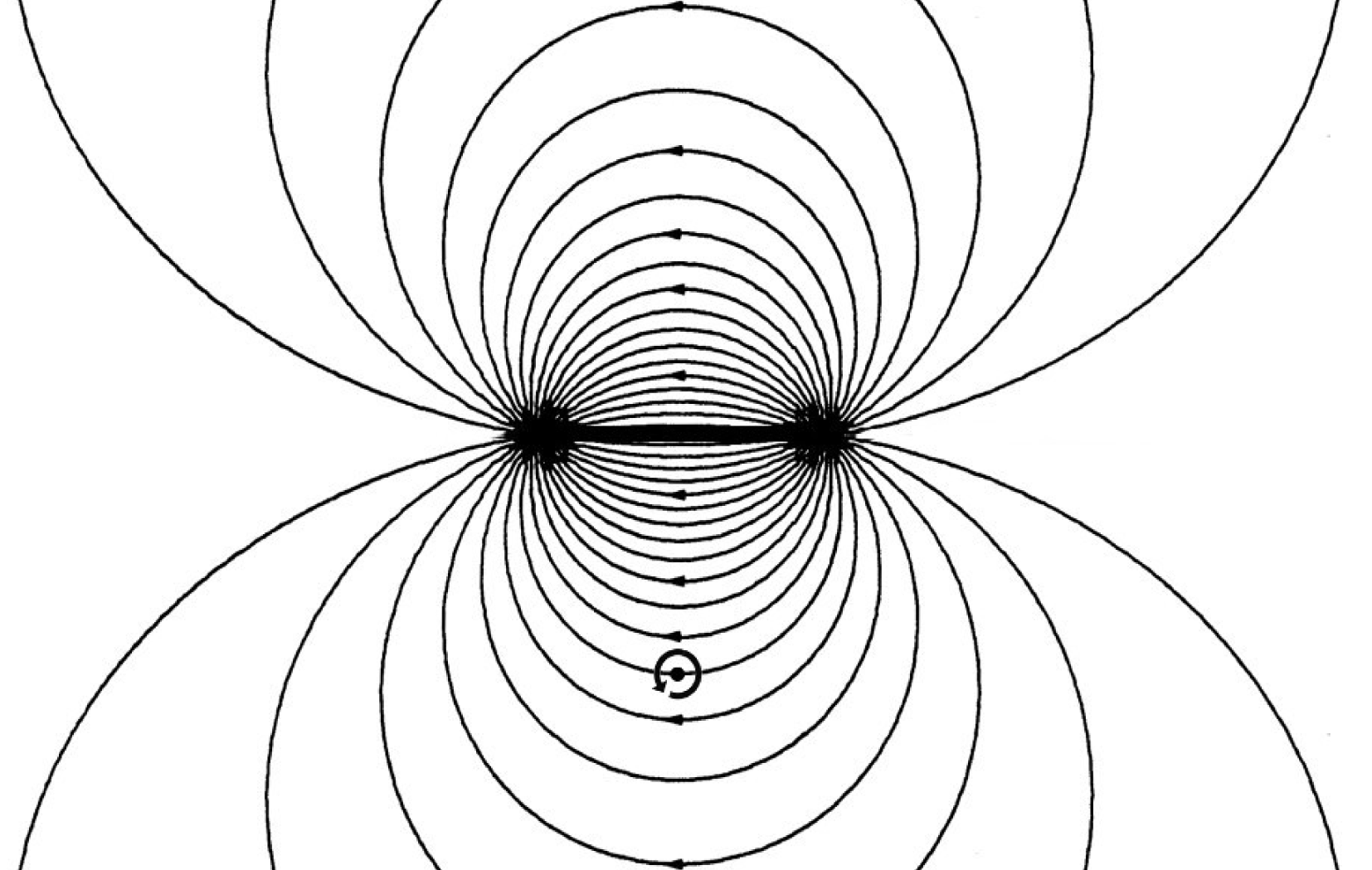
So to obtain the simplest, leading-order version of problem (i), following Reference Bühler and McIntyreBM03, we let the unrefracted wavetrain extend between wave source and sink regions centred at finite locations
 $(x,y)=(-X,Y)$
and
 $(+X,Y)$
, say, as sketched in figure 4 (heavy straight line). For consistency with Reference Bühler and McIntyreBM03’s use of ray theory we take
 $X,Y\gg W$
, and
 $W\gg k_{0}^{-1}$
, where
 $W$
is a width-scale for the wavetrain. In order to generate and absorb an approximately monochromatic wavetrain, the wave source and sink are prescribed, just as in Reference Bühler and McIntyreBM03, by taking the oscillatory forcing potential
 $\unicode[STIX]{x1D712}^{\prime }$
to be
 $\exp (\text{i}\boldsymbol{k}\!\cdot \boldsymbol{x}-\text{i}kct)$
times a slowly-varying forcing envelope whose length-scale is at least of the same order of magnitude as
 $W$
, and where the real part is understood. However, the forcing envelope scale is kept
 $\ll X,Y$
, allowing us to think of the source and sink regions as approximately localized. It is convenient to take
 $\boldsymbol{k}\!\cdot \boldsymbol{x}=k_{0}x$
in the source along with
 $kct=k_{0}ct$
, with constant
 $k_{0}$
.
The
 $O(a^{2}\unicode[STIX]{x1D716}^{0})$
Bretherton flow for the unrefracted wavetrain satisfies (2.17), with evanescence at infinity. It consists of the Stokes drift
 $\overline{\boldsymbol{u}}^{\text{S}}$
straight along the wavetrain, parallel to
 $\hat{\boldsymbol{x}}$
, together with irrotational return flows symmetrically on both sides, as sketched in figure 4. All the vorticity of this Bretherton flow comes from
 $\hat{\boldsymbol{z}}\!\cdot \unicode[STIX]{x1D735}\!\times \unicode[STIX]{x1D5FD}$
on the right-hand side of (2.17). Within the wavetrain but outside the wave source and sink,
 $\hat{\boldsymbol{z}}\!\cdot \unicode[STIX]{x1D735}\!\times \unicode[STIX]{x1D5FD}$
is simply minus the horizontal shear of the Stokes drift.
Schematic of Bretherton-flow streamlines in problem (i), as analysed in Reference Bühler and McIntyreBM03 correct to lowest order
 $O(a^{2}\unicode[STIX]{x1D716}^{0})$
for the finite wavetrain whose ray path is shown by the heavy straight line. At this order the Stokes drift is non-divergent except within the wave source and sink regions. The waves propagate from a source on the left to a sink on the right.

In virtue of the incompressibility expressed by (2.14)–(2.16), the irrotational return flow outside the wavetrain, which advects the vortex core, is the same as if it were induced by a two-dimensional mass sink at the left end of the wavetrain and a mass source at the right end whose strengths are equal to the mass flow in the Stokes drift within the wavetrain. Omitting factors
 $\unicode[STIX]{x1D70C}$
, where
 $\unicode[STIX]{x1D70C}$
is fluid mass density, we define the source and sink strengths
 $\pm S$
as the volume fluxes in a layer of unit depth; thus
 $$\begin{eqnarray}S=\int \overline{u}^{\text{S}}(\,y)\text{d}y=\int \mathsf{p}_{1}(\,y)\text{d}y,\end{eqnarray}$$
with the integral taken across the wavetrain. The pseudomomentum within the wavetrain has been written correct to
 $O(a^{2}\unicode[STIX]{x1D716}^{0})$
as
 $\mathsf{p}_{1}(\,y)\,\hat{\boldsymbol{x}}$
. Using
 $W\ll X$
and
 $W\ll Y$
, again following Reference Bühler and McIntyreBM03, we can approximate the mass-source flow in problem (i) as radially outward from
 $(x,y)=(X,Y)$
at speed
 $S/[2\unicode[STIX]{x1D70B}\{(x-X)^{2}+{(\,y-Y)^{2}\}}^{1/2}]$
, and similarly the mass-sink flow as radially inward toward
 $(x,y)=(-X,Y)$
. When these flows are added vectorially we obtain the flow pattern sketched in figure 4; and the net velocity advecting the vortex core at
 $(x,y)=(0,0)$
is
 $$\begin{eqnarray}\overline{\boldsymbol{u}}^{\text{L}}(0,0)~=~\frac{S}{\unicode[STIX]{x1D70B}}\frac{X}{X^{2}+Y^{2}}(-\hat{\boldsymbol{x}})\end{eqnarray}$$
correct to
 $O(a^{2}\unicode[STIX]{x1D716}^{0})$
. Because of the Magnus relation this corresponds to a resultant recoil force
 $\boldsymbol{R}=-\unicode[STIX]{x1D6E4}\hat{\boldsymbol{z}}\!\times \overline{\boldsymbol{u}}^{\text{L}}(0,0)$
, i.e.
 $$\begin{eqnarray}\boldsymbol{R}~=~\frac{\unicode[STIX]{x1D6E4}S}{\unicode[STIX]{x1D70B}}\frac{X}{X^{2}+Y^{2}}(+\hat{\boldsymbol{y}})\end{eqnarray}$$
correct to
 $O(a^{2}\unicode[STIX]{x1D716}^{1})$
, where
 $\hat{\boldsymbol{y}}$
is the unit vector in the
 $y$
direction.
Notice that
 $\overline{\boldsymbol{u}}^{\text{L}}(0,0)$
and
 $\boldsymbol{R}$
tend toward zero in the formal limit
 $X\rightarrow \infty$
, cross-checking what was deduced from the direction of
 $\boldsymbol{C}^{\text{abs}}$
and consequent vanishing of the
 $O(a^{2}\unicode[STIX]{x1D716}^{1})$
net pseudomomentum flux and recoil force in that limit. As the wavetrain gets longer, the irrotational return part of the Bretherton flow becomes increasingly spread out in the
 $y$
direction, diluting its effect at
 $(x,y)=(0,0)$
.
5 Bretherton flows and recoil forces for problem (ii)
The dilution effect just pointed out is the easiest way of seeing the non-interchangeability of limits in problem (ii). The same dilution effect occurs for any wavetrain whose width
 $W$
is held fixed while its length
 $L=2X\rightarrow \infty$
. In that formal limit the magnitude of the return flow at any fixed point tends toward zero; and it remains zero if the formal limit
 $W\rightarrow \infty$
is taken subsequently. The vortex core is then advected solely by the Stokes drift
 $\overline{\boldsymbol{u}}^{\text{S}}(0,0)=\overline{\boldsymbol{u}}^{\text{S}}=\mathsf{p}_{1}\hat{\boldsymbol{x}}$
, which is now constant across the wavetrain, so that with
 $L\rightarrow \infty$
first in problem (ii), (4.2) and (4.3) are replaced by
 $$\begin{eqnarray}\overline{\boldsymbol{u}}^{\text{L}}(0,0)~=~\overline{\boldsymbol{u}}^{\text{S}}~=~\mathsf{p}_{1}\hat{\boldsymbol{x}}\end{eqnarray}$$
and
 $$\begin{eqnarray}\boldsymbol{R}~=~-\unicode[STIX]{x1D6E4}\mathsf{p}_{1}\hat{\boldsymbol{y}}.\end{eqnarray}$$
Not only the magnitudes but also the signs have changed. These results hold for arbitrary
 $k_{0}r_{0}$
, because in the unrefracted wavetrain we always have
 $\overline{\boldsymbol{u}}^{\text{S}}=\unicode[STIX]{x1D5FD}=\mathsf{p}_{1}\hat{\boldsymbol{x}}$
. Notice that (5.2) is equal to the Craik–Leibovich vortex force
 $\overline{\boldsymbol{u}}^{\text{S}}\!\times \overline{\unicode[STIX]{x1D74E}}=\overline{\boldsymbol{u}}^{\text{S}}\!\times \unicode[STIX]{x1D74E}_{0}$
integrated over the vortex core, corresponding to the Iordanskii force in the quantum fluids literature (e.g. Sonin Reference Sonin1997), with
 $\overline{\boldsymbol{u}}^{\text{S}}=\unicode[STIX]{x1D5FD}$
corresponding to the phonon current per unit mass. The relation to the Aharonov–Bohm effect is discussed in the next two sections.
In any other version of problem (ii) there will be two contributions, one from the Craik–Leibovich vortex force and the other from the return part of the Bretherton flow. In the opposite formal limit, with the width
 $W$
of the wavetrain going to infinity first, the two contributions cancel. The return flow is then uniform, and equal and opposite to the Stokes drift, being diluted only near the extremities
 $y\sim \pm {\textstyle \frac{1}{2}}W$
. In that formal limit, therefore, the recoil force
 $\boldsymbol{R}$
vanishes.
In all other versions of problem (ii) there is always some dilution, making the return flow weaker than the Stokes drift and keeping the sign of the recoil opposite to that in problem (i). For instance, consider the ‘square’ limit
 $L=W\rightarrow \infty$
. Then it is readily shown that
 $$\begin{eqnarray}\overline{\boldsymbol{u}}^{\text{L}}(0,0)~=~{\textstyle \frac{1}{2}}\overline{\boldsymbol{u}}^{\text{S}}(0,0)~=~{\textstyle \frac{1}{2}}\mathsf{p}_{1}\hat{\boldsymbol{x}}\end{eqnarray}$$
so that in place of (5.2) we have
 $$\begin{eqnarray}\boldsymbol{R}~=~-{\textstyle \frac{1}{2}}\unicode[STIX]{x1D6E4}\mathsf{p}_{1}\hat{\boldsymbol{y}}.\end{eqnarray}$$
More generally, the factor
 ${\textstyle \frac{1}{2}}$
is replaced by
 $\{1-\,2\unicode[STIX]{x1D70B}^{-1}\lim \arctan (W/L)\}$
.
To derive this last result, one can regard the wide wavetrain as made up of narrow wavetrains each with
 $S=\mathsf{p}_{1}\text{d}y$
, for constant
 $\mathsf{p}_{1}$
, and then integrate (4.3), with
 $Y$
replaced by
 $y$
, over the whole wavetrain to get the contribution to
 $\boldsymbol{R}$
from the return flow. That contribution, for
 $L\rightarrow \infty$
and
 $W\rightarrow \infty$
in various ways, is therefore
 $$\begin{eqnarray}\frac{\unicode[STIX]{x1D6E4}\mathsf{p}_{1}}{\unicode[STIX]{x1D70B}}\lim \int _{-{\textstyle \frac{1}{2}}W}^{{\textstyle \frac{1}{2}}W}\frac{X\text{d}y}{X^{2}+y^{2}}(+\hat{\boldsymbol{y}})\;=\;\frac{2\unicode[STIX]{x1D6E4}\mathsf{p}_{1}}{\unicode[STIX]{x1D70B}}\lim \arctan (W/L)\,\hat{\boldsymbol{y}}.\end{eqnarray}$$
In the next two sections, the foregoing results for problem (ii) will be cross-checked against computations of far-field pseudomomentum fluxes correct to
 $O(a^{2}\unicode[STIX]{x1D716}^{1})$
, taking account of the refracted wavecrest shapes illustrated in figure 2 and their mathematical description (1.2). The impulse–pseudomomentum theorem tells us that the results must agree; but it is interesting, nevertheless, not only to carry out the cross-checks but also to see how the refraction works in more detail, thereby gaining mechanistic insight, and another view of the non-interchangeability of limits.
Perhaps surprisingly, the quantum fluids literature – going back over the past fifty years or so – tends to ignore many of the points under discussion, including the
 $O(a^{2})$
mean flow problem, the distinction between momentum and pseudomomentum, and the non-interchangeability of limits. The author has, however, found one big quantum fluids paper (Sonin Reference Sonin1997) in which the non-interchangeability of limits is mentioned toward the end of the paper, almost as an afterthought; see below equation (83) therein. Another paper (Wexler & Thouless Reference Wexler and Thouless1998) takes a different path but flags up the dangers of manipulating divergent infinite series. Some but not all of the
 $O(a^{2})$
effects are discussed in Stone (Reference Stone2000b
), while all are consistently dealt with in Guo & Bühler (Reference Guo and Bühler2014), within the Gross–Pitaevskii superfluid model, but only for problem (i). The issues still seem to be surrounded by controversy, perhaps involving unconscious assumptions (e.g. McIntyre Reference McIntyre2017) about, for instance, the distinction between particles and quasiparticles.
6 Wave refraction in problem (ii): the far field outside the wake
The impulse-pseudomomentum theorem says that
 $\boldsymbol{R}$
can be computed as
 $-\oint \unicode[STIX]{x1D5D5}\!\cdot \hat{\boldsymbol{n}}\text{d}s$
, correct to
 $O(a^{2}\unicode[STIX]{x1D716}^{1})$
, for a steady wave field whose sources and sinks lie outside the contour of integration. The unit normal
 $\hat{\boldsymbol{n}}$
is directed outward, and
 $\unicode[STIX]{x1D5D5}$
is the pseudomomentum flux tensor appearing in (3.4). We take advantage of the simplicity of the refracted far-field solution (1.2), and its compatibility with ray theory and the group-velocity property (3.5), by letting the contour expand appropriately as
 $L\rightarrow \infty$
and
 $W\rightarrow \infty$
. It is convenient to take the contour to be a rectangle with dimensions
 $L$
by
 $W$
, where
 $L$
is now to be read as the length of the wavetrain excluding its source and sink regions, as they recede to infinity. Then, correct to
 $O(a^{2}\unicode[STIX]{x1D716}^{1})$
,
 $$\begin{eqnarray}\boldsymbol{R}\,=\,-\lim \oint \unicode[STIX]{x1D5D5}\!\cdot \hat{\boldsymbol{n}}\text{d}s\;=\,\lim \left(\mathop{\int }_{-\frac{1}{2}W}^{\frac{1}{2}W}\unicode[STIX]{x1D5D5}\!\cdot \hat{\boldsymbol{x}}\text{d}y\biggm\vert_{x=-\frac{1}{2}L}-\int _{-\frac{1}{2}W}^{\frac{1}{2}W}\unicode[STIX]{x1D5D5}\!\cdot \hat{\boldsymbol{x}}\text{d}y\biggm\vert_{x=\frac{1}{2}L}\right).\end{eqnarray}$$
We have used (1.2) and (3.5) to neglect the contributions from the sides of the rectangle parallel to
 $\hat{\boldsymbol{x}}$
, as follows. For the transverse,
 $y$
component, the only relevant component of (3.5) on the sides parallel to
 $\hat{\boldsymbol{x}}$
is
 $\mathsf{B}_{22}=\hat{\boldsymbol{y}}\!\cdot \unicode[STIX]{x1D5FD}\,\boldsymbol{C}^{\text{abs}}\!\cdot \hat{\boldsymbol{y}}$
. In the far field, again thanks to ray theory, we have
 $\unicode[STIX]{x1D5FD}\,=\,\overline{\boldsymbol{u}}^{\text{S}}\,=\,{\mathcal{A}}\boldsymbol{k}$
where
 ${\mathcal{A}}$
is the wave-action per unit mass and where
 $\boldsymbol{k}\,=\,\unicode[STIX]{x1D735}\unicode[STIX]{x1D6F7}\,=\,k_{0}\{\hat{\boldsymbol{x}}-\unicode[STIX]{x1D716}r_{0}r^{-1}\hat{\unicode[STIX]{x1D73D}}+O(\unicode[STIX]{x1D716}^{2}r_{0}^{2}r^{-2})\}$
, from (1.2) and (1.3) or from (2.4). We also have
 $c=c(r)=c_{0}\{1+O(\unicode[STIX]{x1D716}^{2}r_{0}^{2}r^{-2})\}$
, as noted in § 1. Denoting
 $\unicode[STIX]{x1D5FD}\!\cdot \hat{\boldsymbol{x}}$
by
 $\mathsf{p}_{1}$
as before, and
 $\unicode[STIX]{x1D5FD}\!\cdot \hat{\boldsymbol{y}}$
by
 $\mathsf{p}_{2}$
, we have
 $\mathsf{p}_{2}/\mathsf{p}_{1}=\boldsymbol{k}\!\cdot \hat{\boldsymbol{y}}/\boldsymbol{k}\!\cdot \hat{\boldsymbol{x}}=O(\unicode[STIX]{x1D716}r_{0}r^{-1})$
. From the formula (2.8), again noting the cancellation of leading-order
 $y$
components, we have
 $\boldsymbol{C}^{\text{abs}}\!\cdot \hat{\boldsymbol{y}}=O(\unicode[STIX]{x1D716}^{2}c_{0}r_{0}^{2}r^{-2})$
. Hence
 $\mathsf{B}_{22}=\mathsf{p}_{1}c_{0}$
times
 $O(\unicode[STIX]{x1D716}^{3}r_{0}^{3}r^{-3})$
. For the longitudinal,
 $x$
component, we have
 $\mathsf{B}_{12}=\mathsf{p}_{1}\boldsymbol{C}^{\text{abs}}\!\cdot \hat{\boldsymbol{y}}$
 $=\mathsf{p}_{1}c_{0}$
times
 $O(\unicode[STIX]{x1D716}^{2}r_{0}^{2}r^{-2})$
. Both make negligible contributions as the rectangle expands to infinity.
Now it is clear from § 5 that
 $\boldsymbol{R}\Vert \hat{\boldsymbol{y}}$
, so that
 $\boldsymbol{R}=R\hat{\boldsymbol{y}}$
, say, correct to
 $O(a^{2}\unicode[STIX]{x1D716}^{1})$
. For the sake of brevity, therefore, we restrict attention from now on to evaluating
 $R$
from the
 $y$
component of (6.1). We do this in two stages, to be described in this and the next section. The first stage is to compute the contribution
 $R_{\text{o}}$
from outside the wake. The non-interchangeability of limits comes from that contribution. Outside the wake, we can again use (1.2), (2.4), (2.8) and (3.5). At the second stage, in the next section, we compute
 $R=R_{\text{o}}+R_{\text{w}}$
, where
 $R_{\text{w}}$
is the contribution from within the wake. It will be found that
 $R_{\text{w}}$
agrees with (5.2) and that it is proportional to the Aharonov–Bohm phase jump. The first contribution
 $R_{\text{o}}$
will be found to agree with (5.5) and to depend solely on the other relevant refraction effect, the
 $O(\unicode[STIX]{x1D716})$
rotation of wavecrests seen in figure 2 and expressed by the
 $\hat{\unicode[STIX]{x1D73D}}$
term in
 $\boldsymbol{k}$
. From here on we denote
 $\unicode[STIX]{x1D5D5}$
evaluated from (1.2), (2.4), (2.8) and (3.5) by
 $\unicode[STIX]{x1D5D5}_{\text{o}}$
, so that
 $$\begin{eqnarray}R_{\text{o}}=\lim \hat{\boldsymbol{y}}\!\cdot \!\left(\int _{-\frac{1}{2}W}^{\frac{1}{2}W}\unicode[STIX]{x1D5D5}_{\text{o}}\!\cdot \hat{\boldsymbol{x}}\text{d}y\biggm\vert_{x=-\frac{1}{2}L}\!\!-\!\!\int _{-\frac{1}{2}W}^{0-}\unicode[STIX]{x1D5D5}_{\text{o}}\!\cdot \hat{\boldsymbol{x}}\text{d}y\biggm\vert_{x=\frac{1}{2}L}\!\!-\!\!\int _{0+}^{\frac{1}{2}W}\unicode[STIX]{x1D5D5}_{\text{o}}\!\cdot \hat{\boldsymbol{x}}\text{d}y\biggm\vert_{x=\frac{1}{2}L}\right),\end{eqnarray}$$
which, in the limit, correctly excludes the wake contribution because of the relative narrowness of the wake, whose width
 $w\ll W$
, as detailed in the next section.
We can evaluate
 $\hat{\boldsymbol{y}}\!\cdot \unicode[STIX]{x1D5D5}_{\text{o}}\!\cdot \hat{\boldsymbol{x}}=\mathsf{p}_{2}\boldsymbol{C}^{\text{abs}}\!\cdot \hat{\boldsymbol{x}}$
from
 $\boldsymbol{C}^{\text{abs}}\!\cdot \hat{\boldsymbol{x}}=c_{0}\{1+O(\unicode[STIX]{x1D716}r_{0}r^{-1})\}$
and
 $\mathsf{p}_{2}=\mathsf{p}_{1}\boldsymbol{k}\!\cdot \hat{\boldsymbol{y}}/\boldsymbol{k}\!\cdot \hat{\boldsymbol{x}}=-\mathsf{p}_{1}\{\unicode[STIX]{x1D716}r_{0}r^{-1}\hat{\unicode[STIX]{x1D73D}}\!\cdot \hat{\boldsymbol{y}}+O(\unicode[STIX]{x1D716}^{2}r_{0}^{2}r^{-2})\}=\mathsf{p}_{1}k_{0}^{-1}\{\unicode[STIX]{x2202}\unicode[STIX]{x1D6F7}/\unicode[STIX]{x2202}y+O(\unicode[STIX]{x1D716}^{2}r_{0}^{2}r^{-2})\}$
with
 $\unicode[STIX]{x1D6F7}$
as in (1.2), and where
 $\mathsf{p}_{1}$
can now be read as the incident pseudomomentum, neglecting refraction, that is,
 $\mathsf{p}_{1}=$
const. as in §§ 4–5. Correct to
 $O(a^{2}\unicode[STIX]{x1D716}^{1})$
, therefore, the first integral on the right of (6.2) reduces to
 $c_{0}\mathsf{p}_{1}k_{0}^{-1}\lim \int _{-\unicode[STIX]{x1D6FC}\tilde{\unicode[STIX]{x1D703}}}^{+\unicode[STIX]{x1D6FC}\tilde{\unicode[STIX]{x1D703}}}\text{d}\unicode[STIX]{x1D6F7}=c_{0}\mathsf{p}_{1}k_{0}^{-1}\lim (2\unicode[STIX]{x1D6FC}\tilde{\unicode[STIX]{x1D703}})=(\unicode[STIX]{x1D6E4}\mathsf{p}_{1}/\unicode[STIX]{x1D70B})\lim \tilde{\unicode[STIX]{x1D703}}$
, where
 $\tilde{\unicode[STIX]{x1D703}}=\arctan (W/L)>0$
. The non-interchangeability of the limits
 $L\rightarrow \infty$
and
 $W\rightarrow \infty$
is now evident.
At each fixed
 $y$
, and correct to
 $O(a^{2}\unicode[STIX]{x1D716}^{1})$
,
 $\mathsf{p}_{2}$
is an odd function of
 $x$
, and
 $\hat{\boldsymbol{y}}\!\cdot \unicode[STIX]{x1D5D5}_{\text{o}}\!\cdot \hat{\boldsymbol{x}}$
also. Therefore the second and third integrals in (6.2) add up to a contribution equal to that from the first integral, so that altogether
 $$\begin{eqnarray}R_{\text{o}}\;=\;\frac{2\unicode[STIX]{x1D6E4}\mathsf{p}_{1}}{\unicode[STIX]{x1D70B}}\lim \arctan (W/L)\end{eqnarray}$$
correct to
 $O(a^{2}\unicode[STIX]{x1D716}^{1})$
, in agreement with (5.5). Notice incidentally that problem (i) now appears as a trivial variant of the above, obtained by selecting appropriate subsets of rays in cases where ray theory is valid all along the wavetrain.
7 Wave refraction in problem (ii): the far field within the wake
To complete the work on problem (ii) we need to evaluate the remaining contribution to the
 $y$
component of (6.1),
 $$\begin{eqnarray}R_{\text{w}}\;=\;-\lim \int _{\text{wake}}\hat{\boldsymbol{y}}\!\cdot \unicode[STIX]{x1D5D5}_{\text{w}}\!\cdot \hat{\boldsymbol{x}}\text{d}y\biggm\vert_{x=\frac{1}{2}L},\end{eqnarray}$$
and to verify that it agrees with (5.2). Here
 $\unicode[STIX]{x1D5D5}_{\text{w}}$
stands for
 $\unicode[STIX]{x1D5D5}$
within the wake.
We evaluate (7.1) in two cases that are analytically tractable,
 $k_{0}r_{0}\ll 1$
and
 $k_{0}r_{0}\gg 1$
. In the second case we use ray tracing across the vortex core, and in the first we draw on the work of Ford & Llewellyn Smith (Reference Ford and Llewellyn Smith1999), hereafter FLS), who carried out a careful and thorough asymptotic analysis of weak refraction and scattering in that case, building on earlier contributions including that of Sakov (Reference Sakov1993); see also Belyaev & Kopiev (Reference Belyaev and Kopiev2008).
7.1 The long-wave case
 $k_{0}r_{0}\ll 1$

FLS’s results are subject to a severe restriction on the range of
 $\unicode[STIX]{x1D6FC}$
values for which they are valid. From (1.3) we see that
 $\unicode[STIX]{x1D6FC}$
is now the product of two small quantities
 $k_{0}r_{0}$
and
 $\unicode[STIX]{x1D716}$
. The results are nevertheless attractive for our purposes because, when valid, they show that the wake has a simple Fresnel-diffractive structure with width-scale
 $w\sim k_{0}^{-1/2}L^{1/2}\gg k_{0}^{-1}$
, and angular scale asymptotically zero, as
 $L\rightarrow \infty$
. Across the wake there is a smooth phase transition such that the ray-theoretic formulae used in § 6 still hold, including
 $\unicode[STIX]{x1D5FD}\propto \boldsymbol{k}$
and
 $\mathsf{p}_{2}=\mathsf{p}_{1}k_{0}^{-1}\unicode[STIX]{x2202}\unicode[STIX]{x1D6F7}/\unicode[STIX]{x2202}y$
, where
 $\unicode[STIX]{x1D6F7}$
now denotes the phase within the wake, as distinct from the phase given by (1.2). The wave field within the wake still has the form
 $A\exp (\text{i}\unicode[STIX]{x1D6F7})$
, where the amplitude
 $A$
is still real and constant to sufficient accuracy across the wake, with relative error
 $O(\unicode[STIX]{x1D716})$
, and where the phase
 $\unicode[STIX]{x1D6F7}$
increases by
 $2\unicode[STIX]{x1D70B}\unicode[STIX]{x1D6FC}$
going anticlockwise across the wake. Therefore we can evaluate
 $\int \hat{\boldsymbol{y}}\!\cdot \unicode[STIX]{x1D5D5}_{\text{w}}\!\cdot \hat{\boldsymbol{x}}\text{d}y$
across the wake as
 $\int c_{0}\mathsf{p}_{2}\text{d}y=c_{0}\mathsf{p}_{1}k_{0}^{-1}\int \!\text{d}\unicode[STIX]{x1D6F7}=2\unicode[STIX]{x1D70B}\unicode[STIX]{x1D6FC}c_{0}\mathsf{p}_{1}k_{0}^{-1}=\unicode[STIX]{x1D6E4}\mathsf{p}_{1}$
, verifying that (7.1) with its minus sign does agree with (5.2).
FLS’s solution also contains a Born-scattering term with amplitude
 $O(r^{-1/2})$
, which however contributes nothing. The magnitude
 $O(r^{-1})$
of its pseudomomentum flux makes it potentially able to contribute to
 $-\oint \unicode[STIX]{x1D5D5}\!\cdot \hat{\boldsymbol{n}}\text{d}s$
. But for our rectangular contour of integration the contribution to
 $\hat{\boldsymbol{y}}\!\cdot \unicode[STIX]{x1D5D5}\!\cdot \hat{\boldsymbol{n}}$
is an odd function of
 $y$
, which integrates to zero.
The reader who wishes to check the foregoing against FLS in more detail may find the following notes useful. Outside the wake, the leading far-field term in FLS’s solution agrees with the foregoing for any
 $\unicode[STIX]{x1D6FC}\ll 1$
because we then have, from (1.2),
 $$\begin{eqnarray}\displaystyle & & \displaystyle \exp (\text{i}\unicode[STIX]{x1D6F7})~=~\exp (-\text{i}\unicode[STIX]{x1D6FC}\unicode[STIX]{x1D703})\exp \{\text{i}(k_{0}(x-c_{0}t))+\text{const.}\}\nonumber\\ \displaystyle & & \displaystyle ~=~(1-\text{i}\unicode[STIX]{x1D6FC}\unicode[STIX]{x1D703})\exp \{\text{i}(k_{0}(x-c_{0}t))+\text{const.}\}+O(\unicode[STIX]{x1D6FC}^{2}).\end{eqnarray}$$
This agrees with FLS’s (2.14), (2.20) and the leading term in their (5.7), after allowing for their different definition of
 $\unicode[STIX]{x1D703}$
and remembering that our
 $\unicode[STIX]{x1D703}$
jumps from
 $+\unicode[STIX]{x1D70B}$
to
 $-\unicode[STIX]{x1D70B}$
, going anticlockwise across the positive
 $x$
axis. In their dimensionless notation, our
 $\unicode[STIX]{x1D6FC}$
is written as
 $M^{2}\unicode[STIX]{x1D6E4}\unicode[STIX]{x1D714}/2\unicode[STIX]{x1D70B}$
, where their
 $M$
is our
 $\unicode[STIX]{x1D716}$
and their
 $\unicode[STIX]{x1D6E4}\unicode[STIX]{x1D714}/2\unicode[STIX]{x1D70B}$
is our
 $k_{0}r_{0}/\unicode[STIX]{x1D716}$
, all taken positive. The Born scattering term is the next,
 $O(r^{-1/2})$
term in their (5.7), with outgoing waves
 $\propto r^{-1/2}\exp \{\text{i}k_{0}(r-c_{0}t)\}$
. The Fresnel wake is described by their (5.12). The phase transition at fixed
 $x$
is given by the sum
 $C+S$
of two real-valued Fresnel integrals, suitably scaled, and is therefore an odd function of
 $y/w$
, with
 $\unicode[STIX]{x1D6F7}$
asymptoting toward
 $\pm \unicode[STIX]{x1D70B}\unicode[STIX]{x1D6FC}+\text{const}.$
with gentle oscillations on the scale
 $w$
. The factor
 $\exp (-\text{i}\unicode[STIX]{x1D702}^{2})$
in FSL’s (5.11), where
 $\unicode[STIX]{x1D702}^{2}={\textstyle \frac{1}{2}}(\,y/w)^{2}$
, converts a Born-like factor
 $\exp \{\text{i}k_{0}(r-c_{0}t)\}$
into a plane-wave factor
 $\exp \{\text{i}k_{0}(x-c_{0}t)\}$
, to sufficient accuracy within the wake, matching up with our (7.2).
Belyaev & Kopiev (Reference Belyaev and Kopiev2008) reconsider FLS using a different solution technique, that of Aharonov & Bohm (Reference Aharonov and Bohm1959) and Berry et al. (Reference Berry, Chambers, Large, Upstill and Walmsley1980). They also discuss the conceptual issue of whether (1.2) above can usefully be regarded as a plane wave outside the Fresnel wake, in the limit
 $r\rightarrow \infty$
. However, the wave field properties required by the foregoing analysis of the pseudomomentum budget are unaffected. Those properties are, most crucially, the validity of (1.2) outside the wake, the phase continuity across the wake, and the
 $y$
-antisymmetry of the Born contribution to
 $\hat{\boldsymbol{y}}\!\cdot \unicode[STIX]{x1D5D5}\!\cdot \hat{\boldsymbol{n}}$
. And we note again that the analysis is independently confirmed by the end-to-end cross-check from §§ 3–5.
7.2 The short-wave case
$k_{0}r_{0}\gg 1$

We now evaluate (7.1) in the case
 $kr_{0}\gg 1$
, using ray theory. Attention is restricted to the simplest case, the Rankine vortex model in which the core is in solid rotation, with constant angular velocity
 $\unicode[STIX]{x1D6FA}={\textstyle \frac{1}{2}}|\unicode[STIX]{x1D74E}_{0}|=|\boldsymbol{u}_{0}(r)|/r=\unicode[STIX]{x1D6E4}/2\unicode[STIX]{x1D70B}r_{0}^{2}$
, taken positive, i.e. anticlockwise, for definiteness, as in the figures.
Correct to
 $O(\unicode[STIX]{x1D716})$
the rays outside the core and its lee are straight, as already remarked, with absolute group velocities
 $\boldsymbol{C}^{\text{abs}}$
parallel to
 $\hat{\boldsymbol{x}}$
, but slightly rotated wavecrests, as seen in figure 2. Inside the core, the ray-tracing equations, e.g. (2.14) of Reference Bühler and McIntyreBM03, verify what is obvious from rotating the reference frame while keeping the same intrinsic phase and group velocity
 $c=c_{0}\{1+O(\unicode[STIX]{x1D716}^{2})\}$
, namely that the wavenumber vector
 $\boldsymbol{k}$
rotates with angular velocity
 $\unicode[STIX]{x1D6FA}$
as a ray point crosses the core at velocity
 $c_{0}\hat{\boldsymbol{x}}+O(\unicode[STIX]{x1D716})$
. Thus the rays bend slightly to the left as they cross the core into its lee, where they are straight again but no longer quite parallel to the
 $x$
axis. We note that the group velocity
 $\boldsymbol{C}^{\text{abs}}$
rotates twice as fast as
 $\boldsymbol{k}$
, with angular velocity
 $2\unicode[STIX]{x1D6FA}$
, because of the changing
 $O(\unicode[STIX]{x1D716})$
contribution from the
 $y$
component of
 $\boldsymbol{u}_{0}=\unicode[STIX]{x1D6FA}(-y,x)$
in (2.8) as the ray point crosses the core. This and the straightness of the rays outside the core are special cases of the curl-curvature formula mentioned below (2.8). The formula implies generally that, correct to
 $O(\unicode[STIX]{x1D716})$
, the group velocity vector rotates with angular velocity
 $\unicode[STIX]{x1D74E}_{0}=\unicode[STIX]{x1D735}\!\times \boldsymbol{u}_{0}$
.
Rays emerging from the vortex core and forming a wake with a caustic, computed correct to
 $O(\unicode[STIX]{x1D716})$
from the ray-tracing equations. The
 $O(\unicode[STIX]{x1D716})$
deflections are exaggerated in the plot. The rays entering the core, not shown, are initially parallel to the
 $x$
axis at
 $y/r_{0}=0$
,
 $\pm 0.1$
,
 $\pm 0.2$
,
 $\pm 0.3$
,
 $\pm 0.4$
,
 $\pm 0.5$
,
 $\pm 0.6$
,
 $\pm 0.7$
,
 $\pm 0.8$
,
 $\pm 0.9$
,
 $\pm 0.95$
,
 $\pm 0.98$
,
 $\pm 0.995$
,
 $\pm 1$
.

For weak refraction the ray undergoing the greatest deflection is that crossing the widest part of the core, at
 $y=0$
. The rays from
 $-r_{0}<y<0$
therefore splay out slightly, while those from
 $0<y<r_{0}$
cross one another and form a caustic, extending slightly outside the tangent line
 $y=+r_{0}$
, as shown in figure 5 with the deflections exaggerated. A full analysis is beyond our scope here; to evaluate (7.1) we will simply add up the leading-order pseudomomentum fluxes
 $\hat{\boldsymbol{y}}\!\cdot \unicode[STIX]{x1D5D5}_{\text{w}}\!\cdot \hat{\boldsymbol{x}}=c_{0}\mathsf{p}_{2}$
as if carried by each ray independently. This assumes that the refraction term in the
 $O(a^{2}\unicode[STIX]{x1D716}^{1})$
pseudomomentum law (3.4) works in the same way, to leading order at least, whether or not the rays go through a caustic.
The treatment of the ray deflections as small of order
 $\unicode[STIX]{x1D716}$
, and the neglect of diffractive effects, becomes delicate and very restrictive when combined with the formal limit
 $L\rightarrow \infty$
. It will nevertheless yield the correct result, in agreement with (5.2), as will now be shown. The agreement will also lend support to our assumption about (3.4) and caustics.
The following is a shortcut to the results from the ray-tracing equations shown in figure 5, using the rotation-rate of
 $\boldsymbol{k}$
already mentioned. A ray point entering the core at
 $y=-r_{0}\sin \unicode[STIX]{x1D703}$
, say, for some fixed
 $\unicode[STIX]{x1D703}$
with
 $|\unicode[STIX]{x1D703}|<\unicode[STIX]{x1D70B}/2$
, already has a wavenumber with non-vanishing
 $y$
component
 $\boldsymbol{k}\!\cdot \hat{\boldsymbol{y}}=-\unicode[STIX]{x1D6FC}r_{0}^{-1}\hat{\unicode[STIX]{x1D73D}}\!\cdot \hat{\boldsymbol{y}}=+\unicode[STIX]{x1D6FC}r_{0}^{-1}\cos \unicode[STIX]{x1D703}$
, from (1.2) or (2.4) giving, at that location,
 $\hat{\boldsymbol{y}}\!\cdot \unicode[STIX]{x1D5D5}_{\text{w}}\!\cdot \hat{\boldsymbol{x}}=c_{0}\mathsf{p}_{2}=c_{0}\mathsf{p}_{1}k_{0}^{-1}\unicode[STIX]{x1D6FC}r_{0}^{-1}\cos \unicode[STIX]{x1D703}=\mathsf{p}_{1}\unicode[STIX]{x1D6E4}(2\unicode[STIX]{x1D70B}r_{0})^{-1}\!\cos \unicode[STIX]{x1D703}=\mathsf{p}_{1}\unicode[STIX]{x1D6FA}r_{0}\cos \unicode[STIX]{x1D703}$
. As the ray point crosses the core, over a distance
 $2r_{0}\cos \unicode[STIX]{x1D703}$
and taking a time
 $2c_{0}^{-1}r_{0}\cos \unicode[STIX]{x1D703}$
, the vectors
 $\boldsymbol{k}$
and
 $\unicode[STIX]{x1D5FD}$
rotate with angular velocity
 $\unicode[STIX]{x1D6FA}$
, so that
 $c_{0}\mathsf{p}_{2}$
increases by a further small amount
 $2\mathsf{p}_{1}\unicode[STIX]{x1D6FA}r_{0}\cos \unicode[STIX]{x1D703}$
(equal to
 $c_{0}\mathsf{p}_{1}$
times the net rotation angle
 $2c_{0}^{-1}\unicode[STIX]{x1D6FA}r_{0}\cos \unicode[STIX]{x1D703}$
), and again by a further small amount
 $\mathsf{p}_{1}\unicode[STIX]{x1D6FA}r_{0}\cos \unicode[STIX]{x1D703}$
after exiting the core and reaching sufficiently large
 $x>0$
. This last increment is the same increment as in (1.2) between the far edge of the core and
 $x\rightarrow \infty$
. However, it is to be added to the new far-core-edge value
 $3\mathsf{p}_{1}\unicode[STIX]{x1D6FA}r_{0}\cos \unicode[STIX]{x1D703}$
rather than to the original value
 $-\mathsf{p}_{1}\unicode[STIX]{x1D6FA}r_{0}\cos \unicode[STIX]{x1D703}$
implied by (1.2) and (2.4). With our ray still nearly parallel to the
 $x$
axis after exiting the core, we are using the fact that the
 $O(\unicode[STIX]{x1D716})$
rates of change of
 $\boldsymbol{k}\!\cdot \hat{\boldsymbol{y}}$
outside the core are the same as those implied by (1.2), (2.4) and (2.8).
So, adding all the contributions just noted, we have that the ray has a total end-to-end change
 $\mathsf{p}_{1}\unicode[STIX]{x1D6FA}r_{0}\cos \unicode[STIX]{x1D703}+2\mathsf{p}_{1}\unicode[STIX]{x1D6FA}r_{0}\cos \unicode[STIX]{x1D703}+\mathsf{p}_{1}\unicode[STIX]{x1D6FA}r_{0}\cos \unicode[STIX]{x1D703}=4\mathsf{p}_{1}\unicode[STIX]{x1D6FA}r_{0}\cos \unicode[STIX]{x1D703}$
, in
 $c_{0}\mathsf{p}_{2}$
, corresponding to an end-to-end deflection angle
 $\unicode[STIX]{x1D6FD}$
, say,
 $=\mathsf{p}_{2}/\mathsf{p}_{1}|_{x\rightarrow \infty }=4c_{0}^{-1}\unicode[STIX]{x1D6FA}r_{0}\cos \unicode[STIX]{x1D703}=4\unicode[STIX]{x1D716}\cos \unicode[STIX]{x1D703}$
, with maximum value
 $4\unicode[STIX]{x1D716}$
, in an anticlockwise sense. Integrating the change in
 $c_{0}\mathsf{p}_{2}$
over all the rays that cross the core, from
 $y=-r_{0}$
to
 $y=r_{0}$
, noting that
 $\text{d}y=-r_{0}\cos \unicode[STIX]{x1D703}\text{d}\unicode[STIX]{x1D703}$
and that
 $\int _{-\unicode[STIX]{x1D70B}/2}^{\unicode[STIX]{x1D70B}/2}\cos ^{2}\unicode[STIX]{x1D703}\text{d}\unicode[STIX]{x1D703}=\unicode[STIX]{x1D70B}/2$
, we find from (7.1) with due care over signs that
 $R_{\text{w}}=-2\unicode[STIX]{x1D70B}\mathsf{p}_{1}\unicode[STIX]{x1D6FA}r_{0}^{2}=-\unicode[STIX]{x1D6E4}\mathsf{p}_{1}$
, agreeing with (5.2) as expected.
To summarize, (6.1) gives us, both for
 $k_{0}r_{0}\ll 1$
and for
 $k_{0}r_{0}\gg 1$
,
 $$\begin{eqnarray}R\;=\;R_{\text{w}}+\,R_{\text{o}}\;=\;-\left\{1-\frac{2}{\unicode[STIX]{x1D70B}}\lim \arctan \left(\frac{W}{L}\right)\right\}\unicode[STIX]{x1D6E4}\mathsf{p}_{1}\end{eqnarray}$$
for arbitrary limiting values of
 $W/L$
, agreeing with the independent derivations in §§ 3–5. Furthermore, recalling that those independent derivations are valid for arbitrary
 $k_{0}r_{0}$
, we see also that (7.3) must be a result far more robust than is suggested by the delicacy of the flux computations for
 $k_{0}r_{0}\ll 1$
and
 $k_{0}r_{0}\gg 1$
. On the other hand, everything still depends on the smallness of
 $\unicode[STIX]{x1D716}$
. Numerical solutions for cases of stronger refraction show wakes oriented at substantial angles away from the
 $x$
axis; see for instance figures 2–3 of Coste, Lund & Umeki (Reference Coste, Lund and Umeki1999). And it is still an open question as to what might or might not replace the impulse–pseudomomentum theorem for arbitrary
 $\unicode[STIX]{x1D716}$
.
8 Problem (iii)
The main reason for being interested in this rapidly-rotating version of problem (i), in which the waves are deep-water gravity waves, is the existence of the Ursell anti-Stokes flow. This is an Eulerian-mean flow
 $\overline{\boldsymbol{u}}$
that largely cancels the strongly
 $z$
-dependent Stokes drift
 $\overline{\boldsymbol{u}}^{\text{S}}$
of the waves. Indeed the cancellation is exact, for finite-amplitude waves, when the wave field is exactly steady and exactly homogeneous across an infinite
 $xy$
domain (Ursell Reference Ursell1950; Pollard Reference Pollard1970). (In a thought-experiment starting with irrotational waves, in such a domain, the mean flow undergoes a free inertial oscillation about the anti-Stokes state. It is sometimes forgotten that this thought-experiment was clearly analysed and understood in Ursell’s pioneering work.) In problem (iii), however, contrary to what might at first be thought, the anti-Stokes flow fails to suppress remote recoil.
We consider an unstratified rapidly-rotating system of finite depth
 $H$
under gravity
 $-g\hat{\boldsymbol{z}}$
, so that the
 $z$
direction is vertically upward. The vector Coriolis parameter
 $\boldsymbol{f}$
is parallel to
 $\hat{\boldsymbol{z}}$
. The waves have a wavenumber
 $k=|\boldsymbol{k}|$
that is large enough to make
 $\exp (-kH)$
negligible. The intrinsic wave frequency
 $kc=(gk)^{1/2}\gg f=|\,\boldsymbol{f}|$
, so that rotation affects the wave dynamics only weakly.
In addition to
 $a$
and
 $\unicode[STIX]{x1D716}$
we now have another small parameter, the mean-flow Rossby number
 $$\begin{eqnarray}\text{Ro}~=~U/fr_{0}~\ll ~1,\end{eqnarray}$$
whose smallness will bring in the Taylor–Proudman effect and give us quasigeostrophic mean-flow dynamics. As before, the velocity scale
 $U$
will be taken as the velocity of the vortex flow at the edge of the core,
 $r=r_{0}$
. The core will be defined by non-vanishing quasigeostrophic potential vorticity,
 $(\unicode[STIX]{x1D6FB}_{\!\text{H}}^{2}-L_{\text{D}}^{-2})\tilde{\unicode[STIX]{x1D713}}_{0}$
in the notation of § 2.
The anti-Stokes flow can be regarded as a consequence of the Taylor–Proudman effect together with the exact advection property expressed by the mean vorticity equations (2.10) and (2.11). This is no more than a rephrasing of Ursell’s original argument, putting it within the GLM framework. Focusing on the present case
 $\text{Ro}\ll 1$
, we can regard inertia waves as fast waves with a strong Coriolis restoring force. The Taylor–Proudman effect arises from the corresponding stiffness of the lines of absolute vorticity
 $\boldsymbol{f}+\widetilde{\unicode[STIX]{x1D74E}}$
, which must tend to stay vertical, on average at least. In particular, they cannot be continually sheared over by the mean flow; and for this purpose the mean flow is the Lagrangian-mean flow
 $\overline{\boldsymbol{u}}^{\text{L}}$
, as equations (2.10) and (2.11) make clear. A Lagrangian-mean flow without vertical shear is a Stokes drift plus an Eulerian-mean anti-Stokes flow, plus an additional contribution that is independent of
 $z$
– in this case the vortex flow plus the Bretherton flow that mediates remote recoil.
To tackle problem (iii) we must first derive (2.18). The starting point is the vertical component of (2.11). Writing
 $f+\widetilde{\unicode[STIX]{x1D714}}$
for the vertical component of
 $\boldsymbol{f}+\widetilde{\unicode[STIX]{x1D74E}}$
, and
 $\overline{w}^{\text{L}}$
for the vertical component of
 $\overline{\boldsymbol{u}}^{\text{L}}$
, we have
 $$\begin{eqnarray}\frac{\overline{\text{D}}^{\text{L}}\widetilde{\unicode[STIX]{x1D714}}}{\text{D}t}~+~(f+\widetilde{\unicode[STIX]{x1D714}})\unicode[STIX]{x1D735}\!\cdot \overline{\boldsymbol{u}}^{\text{L}}~=~(\,\boldsymbol{f}+\widetilde{\unicode[STIX]{x1D74E}})\!\cdot \unicode[STIX]{x1D735}\overline{w}^{\text{L}}\end{eqnarray}$$
exactly. Upon cancelling a pair of terms in
 $\unicode[STIX]{x2202}\overline{w}^{\text{L}}/\unicode[STIX]{x2202}z$
, this reduces to
 $$\begin{eqnarray}\frac{\overline{\text{D}}^{\text{L}}\widetilde{\unicode[STIX]{x1D714}}}{\text{D}t}~+~(f+\widetilde{\unicode[STIX]{x1D714}})\unicode[STIX]{x1D735}_{\!\text{H}}^{\phantom{L}}\!\cdot \overline{\boldsymbol{u}}_{\text{H}}^{\text{L}}~=~\widetilde{\unicode[STIX]{x1D74E}}_{\text{H}}\!\cdot \unicode[STIX]{x1D735}_{\!\text{H}}^{\phantom{L}}\overline{w}^{\text{L}}.\end{eqnarray}$$
As before, suffix H denotes horizontal projection. Writing
 $\widetilde{\unicode[STIX]{x1D714}}=\unicode[STIX]{x1D714}_{0}+\widetilde{\unicode[STIX]{x1D714}}_{\text{B}}$
and
 $\overline{\boldsymbol{u}}^{\text{L}}=\boldsymbol{u}_{0}+\overline{\boldsymbol{u}}_{\text{B}}^{\text{L}}$
where the vortex-only contributions
 $\unicode[STIX]{x1D714}_{0}$
and
 $\boldsymbol{u}_{0}$
are
 $z$
-independent, with
 $\boldsymbol{u}_{0}$
horizontal, and the wave-induced contributions
 $\widetilde{\unicode[STIX]{x1D714}}_{\text{B}}$
and
 $\overline{\boldsymbol{u}}_{\text{B}}^{\text{L}}$
are
 $O(a^{2})$
, we note that in the first term on the left the contribution
 $\overline{\boldsymbol{u}}_{\text{B}}^{\text{L}}\!\cdot \unicode[STIX]{x1D735}\widetilde{\unicode[STIX]{x1D714}}_{\text{B}}\,=\,\overline{\boldsymbol{u}}_{\text{B}}^{\text{L}}\!\cdot \unicode[STIX]{x1D735}_{\!\text{H}}^{\phantom{L}}\widetilde{\unicode[STIX]{x1D714}}_{\text{B}}\,+\,\overline{w}^{\text{L}}\unicode[STIX]{x2202}\widetilde{\unicode[STIX]{x1D714}}_{\text{B}}/\unicode[STIX]{x2202}z\,=\,$
 $O(a^{4})$
and is therefore negligible. (We need not restrict
 $\unicode[STIX]{x1D716}$
at this stage.) There are two further such
 $O(a^{4})$
contributions in (8.3), namely the right-hand side, and on the left
 $\widetilde{\unicode[STIX]{x1D714}}_{\text{B}}\unicode[STIX]{x1D735}_{\!\text{H}}^{\phantom{L}}\!\cdot \overline{\boldsymbol{u}}_{\text{H}}^{\text{L}}=\widetilde{\unicode[STIX]{x1D714}}_{\text{B}}\unicode[STIX]{x1D735}_{\!\text{H}}^{\phantom{L}}\!\cdot \overline{\boldsymbol{u}}_{\text{B}}^{\text{L}}$
since
 $\unicode[STIX]{x1D735}_{\!\text{H}}^{\phantom{L}}\!\cdot \boldsymbol{u}_{0}=0$
. The
 $O(a^{2})$
contribution
 $\unicode[STIX]{x1D714}_{0}\unicode[STIX]{x1D735}_{\!\text{H}}^{\phantom{L}}\!\cdot \overline{\boldsymbol{u}}_{\text{H}}^{\text{L}}=\unicode[STIX]{x1D714}_{0}\unicode[STIX]{x1D735}_{\!\text{H}}^{\phantom{L}}\!\cdot \overline{\boldsymbol{u}}_{\text{B}}^{\text{L}}$
is also negligible, against
 $f\unicode[STIX]{x1D735}_{\!\text{H}}^{\phantom{L}}\!\cdot \overline{\boldsymbol{u}}_{\text{H}}^{\text{L}}$
, because of the smallness of
 $\text{Ro}$
. After neglecting all these contributions we can take the vertical average of (8.3), using the
 $z$
-independence of
 $\boldsymbol{u}_{0}$
and
 $\unicode[STIX]{x1D74E}_{0}$
. Denoting vertical averages by angle brackets as before and noting that
 $\boldsymbol{u}_{0}\!\cdot \unicode[STIX]{x1D735}_{\!\text{H}}^{\phantom{L}}\unicode[STIX]{x1D714}_{0}=0$
we get
 $$\begin{eqnarray}\left(\frac{\unicode[STIX]{x2202}}{\unicode[STIX]{x2202}t}+\boldsymbol{u}_{0}\!\cdot \unicode[STIX]{x1D735}_{\!\text{H}}^{\phantom{L}}\right)\langle \widetilde{\unicode[STIX]{x1D714}}_{\text{B}}\rangle \;+\;\langle \overline{\boldsymbol{u}}_{\text{B}}^{\text{L}}\rangle \!\cdot \unicode[STIX]{x1D735}_{\!\text{H}}^{\phantom{L}}\unicode[STIX]{x1D714}_{0}\;+\;f\unicode[STIX]{x1D735}_{\!\text{H}}^{\phantom{L}}\!\cdot \langle \overline{\boldsymbol{u}}_{\text{H}}^{\text{L}}\rangle ~=~0\end{eqnarray}$$
or, written more compactly, again with negligible error
 $O(a^{4})$
,
 $$\begin{eqnarray}\frac{\overline{\text{D}}_{\text{H}}^{\text{L}}\langle \widetilde{\unicode[STIX]{x1D714}}\rangle }{\text{D}t}~+~f\unicode[STIX]{x1D735}_{\!\text{H}}^{\phantom{L}}\!\cdot \langle \overline{\boldsymbol{u}}_{\text{H}}^{\text{L}}\rangle ~=~0,\end{eqnarray}$$
where we have defined
 $\overline{\text{D}}_{\text{H}}^{\text{L}}/\text{D}t=\unicode[STIX]{x2202}/\unicode[STIX]{x2202}t+\langle \overline{\boldsymbol{u}}_{\text{H}}^{\text{L}}\rangle \!\cdot \unicode[STIX]{x1D735}_{\!\text{H}}^{\phantom{L}}$
. In a closely similar way, the vertical average of the three-dimensional mass-conservation equation, Reference BühlerB14 equation (10.47), simplifies to a vertically-averaged version of (2.13),
 $$\begin{eqnarray}\frac{\overline{\text{D}}_{\text{H}}^{\text{L}}\tilde{h}}{\text{D}t}~+~\tilde{h}\unicode[STIX]{x1D735}_{\!\text{H}}^{\phantom{L}}\!\cdot \langle \overline{\boldsymbol{u}}_{\text{H}}^{\text{L}}\rangle ~=~0,\end{eqnarray}$$
again with negligible error
 $O(a^{4})$
. As before, the mean layer depth
 $\tilde{h}=\tilde{h}(x,y,t)$
is defined such that
 $\unicode[STIX]{x1D70C}\tilde{h}\text{d}x\,\text{d}y$
is the areal mass element, where
 $\unicode[STIX]{x1D70C}$
is the constant mass density. Elimination of
 $\unicode[STIX]{x1D735}_{\!\text{H}}^{\phantom{L}}\!\cdot \langle \overline{\boldsymbol{u}}_{\text{H}}^{\text{L}}\rangle$
between (8.5) and (8.6) gives us that
 $\langle \widetilde{\unicode[STIX]{x1D714}}\rangle -f\ln \tilde{h}$
, plus an arbitrary additive constant, is a material invariant under advection by
 $\langle \overline{\boldsymbol{u}}_{\text{H}}^{\text{L}}\rangle$
. Fractional changes in
 $\tilde{h}$
are small,
 $(\tilde{h}-H)/H=O(\text{Ro})$
, and so taking the additive constant to be
 $f\ln H$
and using
 $\ln \tilde{h}-\ln H=\ln (\tilde{h}/H)=\ln \{(\tilde{h}-H+H)/H\}=(\tilde{h}-H)/H+O(\text{Ro}^{2})$
, we get
 $$\begin{eqnarray}\frac{\overline{\text{D}}_{\text{H}}^{\text{L}}\tilde{q}}{\text{D}t}~=~0,\end{eqnarray}$$
where
 $$\begin{eqnarray}\tilde{q}~=~\tilde{q}(x,y,t)~=~\langle \widetilde{\unicode[STIX]{x1D714}}\rangle -\frac{f}{H}(\tilde{h}-H),\end{eqnarray}$$
which is the appropriate form of the quasigeostrophic potential vorticity of the mean flow. In any thought-experiment in which the waves are switched on after the vortex is established, (8.7) implies that the
 $\tilde{q}$
field is unchanged by the presence of the waves, apart from the advection of the vortex core by the Bretherton flow. See also appendix B. So in problem (iii) we have
 $\tilde{q}=q_{0}$
where
 $q_{0}$
is the potential vorticity of the vortex alone.
The final step in deriving (2.18) is to make explicit use of hydrostatic and geostrophic balance. Some delicate scale analysis is involved at this stage. The full details are given in appendix C, in which the key points are as follows. Hydrostatic balance, meaning the overall balance for a complete fluid column, implies that horizontal pressure gradients on the bottom, underneath the wavetrain, are given by
 $\unicode[STIX]{x1D70C}g\unicode[STIX]{x1D735}_{\!\text{H}}^{\phantom{L}}\tilde{h}$
, again because
 $\unicode[STIX]{x1D70C}\tilde{h}\text{d}x\,\text{d}y$
is the areal mass element. Geostrophic balance then gives (2.15) with
 $\tilde{\unicode[STIX]{x1D713}}=g(\tilde{h}-H)/f$
. Then
 $\tilde{q}=q_{0}$
together with (2.9) and (2.16) gives (2.18). The Taylor–Proudman effect extends the geostrophic relation upward into the wavetrain,
 $\langle \overline{\boldsymbol{u}}_{\text{H}}^{\text{L}}\rangle =\overline{\boldsymbol{u}}_{\text{H}}^{\text{L}}$
. Radiation stresses within the wavetrain cannot break the overall hydrostatic balance because such stresses have no foothold on the bottom boundary, in virtue of our assumption that
 $\exp (-kH)$
is negligibly small. That allows us to neglect the net vertical, radiation-stress-induced external force on the fluid column – in contrast, it should be noted, with the situation of figure 3. For further comments see appendix C. In appendix C we also note that the exact wave solution of Pollard (Reference Pollard1970) provides some useful cross-checks.
With (2.18) in place, we can now invoke the impulse-pseudomomentum theorem to assert that recoil forces can be computed either from Bretherton flows correct to
 $O(a^{2}\unicode[STIX]{x1D716}^{0})$
or from net pseudomomentum fluxes correct to
 $O(a^{2}\unicode[STIX]{x1D716}^{1})$
. In the remainder of this section we carry out both computations, in the case of a small vortex core with
 $r_{0}\ll L_{\text{D}}$
, providing mechanistic insight as well as an end-to-end cross-check on our derivation of (2.18).
First consider the Bretherton flow. Because it satisfies (2.18), it decays sideways like
 $\exp (-|y|/L_{\text{D}})$
, on the fixed length-scale
 $L_{\text{D}}$
. Therefore there is no dilution effect like that in problem (i). With
 $L\rightarrow \infty$
, and with a narrow wavetrain for which
 $W\ll L_{\text{D}}$
and
 $W\ll Y$
, in the notation of § 4, we have, for
 $|y-Y|>W$
, outside the unrefracted wavetrain, with
 $Y$
the distance to the vortex core,
 $$\begin{eqnarray}\overline{\boldsymbol{u}}_{\text{B}}^{\text{L}}(x,y)~=~(S/2L_{\text{D}})\exp (-|y-Y|/L_{\text{D}})(-\hat{\boldsymbol{x}}),\end{eqnarray}$$
where
 $S$
is still defined by (4.1) but with vertical averaging understood. So, for our small vortex core with
 $r_{0}\ll L_{\text{D}}$
, carried bodily by the
 $z$
-independent Bretherton flow, the recoil force is
 $$\begin{eqnarray}\boldsymbol{R}=(\unicode[STIX]{x1D6E4}S/2L_{\text{D}})\exp (-|Y|/L_{\text{D}})(+\hat{\boldsymbol{y}}),\end{eqnarray}$$
with
 $\unicode[STIX]{x1D6E4}$
evaluated at the edge of the core. The signs are the same as those in problem (i).
Second, we compute
 $\boldsymbol{R}$
from the
 $O(a^{2}\unicode[STIX]{x1D716}^{1})$
pseudomomentum flux
 $\mathsf{B}_{21}=\hat{\boldsymbol{y}}\!\cdot \unicode[STIX]{x1D5D5}\!\cdot \hat{\boldsymbol{x}}$
, using ray theory. As in § 7.2, the rays start exactly parallel to the
 $x$
axis, with
 $\mathsf{p}_{2}\rightarrow 0$
as
 $x\rightarrow -\infty$
, and finish after bending slightly, through an
 $O(\unicode[STIX]{x1D716})$
end-to-end deflection angle
 $\unicode[STIX]{x1D6FD}=\mathsf{p}_{2}/\mathsf{p}_{1}|_{x\rightarrow \infty }$
. The vortex flow has velocity
 $\boldsymbol{u}_{0}(r)=\hat{\unicode[STIX]{x1D73D}}\unicode[STIX]{x2202}\unicode[STIX]{x1D713}_{0}/\unicode[STIX]{x2202}r$
, say, where the quasigeostrophic streamfunction
 $\unicode[STIX]{x1D713}_{0}$
satisfies
 $(\unicode[STIX]{x1D6FB}^{2}-L_{\text{D}}^{-2})\unicode[STIX]{x1D713}_{0}=0$
outside the core. Defining
 $r^{\prime }=r/L_{\text{D}}$
, we have
 $$\begin{eqnarray}\unicode[STIX]{x1D713}_{0}~=\;-\frac{\unicode[STIX]{x1D6E4}}{2\unicode[STIX]{x1D70B}}K_{0}(r^{\prime })\quad \text{outside the core},\end{eqnarray}$$
where
 $K_{0}(r^{\prime })$
is the modified Bessel function asymptoting to
 $(\unicode[STIX]{x1D70B}/2r^{\prime })^{1/2}\exp (-r^{\prime })$
for
 $r^{\prime }\gg 1$
and to
 $-\ln (r^{\prime })$
for
 $r^{\prime }\ll 1$
, near the core. The Kelvin circulation
 $\unicode[STIX]{x1D6E4}$
is again defined to be the circulation at the core edge
 $r=r_{0}$
, namely
 $\pm 2\unicode[STIX]{x1D70B}r_{0}|\boldsymbol{u}_{0}(r_{0})|=\pm 2\unicode[STIX]{x1D70B}r_{0}U$
, with positive sign when the vortex is cyclonic as in the figures. For
 $r>r_{0}$
the circulation is not constant, but decays exponentially like
 $r^{\prime 1/2}\exp (-r^{\prime })$
.
To verify agreement with (8.10) we need only calculate
 $\unicode[STIX]{x1D6FD}$
. The curl-curvature formula tells us that
 $\unicode[STIX]{x1D6FD}$
is non-zero at
 $O(\unicode[STIX]{x1D716})$
, because the relative vorticity
 $\unicode[STIX]{x1D6FB}^{2}\unicode[STIX]{x1D713}_{0}=L_{\text{D}}^{-2}\unicode[STIX]{x1D713}_{0}$
is non-zero outside the core. A cyclonic vortex core is surrounded by anticyclonic vorticity and the rays therefore bend to the right, rather than to the left as in § 7, so that
 $\text{sgn}\unicode[STIX]{x1D6FD}=-\text{sgn}\unicode[STIX]{x1D6E4}$
. Notice incidentally that there will no longer be any far-field subtleties, or issues with non-interchangeable limits, thanks to the exponential decay of
 $\unicode[STIX]{x1D713}_{0}$
. Another effect of that decay is that the right-bending rays must splay out slightly when they pass to the left of the vortex, but cross one another and form a caustic when to the right. The presence or absence of a caustic makes no difference to the results.
The deep water waves in problem (iii) have intrinsic frequency
 $kc=(gk)^{1/2}$
and intrinsic group velocity
 $\boldsymbol{C}=C\boldsymbol{k}/k$
where
 $C={\textstyle \frac{1}{2}}c={\textstyle \frac{1}{2}}(g/k)^{1/2}$
. The absolute group velocity
 $\boldsymbol{C}^{\text{abs}}={\textstyle \frac{1}{2}}c_{0}\hat{\boldsymbol{x}}+$
 $O(\unicode[STIX]{x1D716})$
, with
 $O(\unicode[STIX]{x1D716})$
contributions coming both from
 $\boldsymbol{u}_{0}$
and from refractive changes in wavenumber
 $\boldsymbol{k}$
. Following a ray point moving at speed
 ${\textstyle \frac{1}{2}}c_{0}+$
 $O(\unicode[STIX]{x1D716})$
, the curl-curvature formula says that the direction of
 $\boldsymbol{C}^{\text{abs}}$
rotates clockwise away from the
 $x$
direction at an angular velocity equal to the (negative) relative vorticity
 $\unicode[STIX]{x1D6FB}^{2}\unicode[STIX]{x1D713}_{0}=L_{\text{D}}^{-2}\unicode[STIX]{x1D713}_{0}$
. So for weak refraction we have
 $$\begin{eqnarray}\unicode[STIX]{x1D6FD}~=~({\textstyle \frac{1}{2}}c_{0})^{-1}\int _{-\infty }^{\infty }L_{\text{D}}^{-2}\unicode[STIX]{x1D713}_{0}(x,Y)\text{d}x~=\;-\frac{\unicode[STIX]{x1D6E4}\;}{\unicode[STIX]{x1D70B}c_{0}L_{\text{D}}^{2}}\int _{-\infty }^{\infty }K_{0}\{(x^{2}+Y^{2})^{1/2}/L_{\text{D}}\}\text{d}x.\end{eqnarray}$$
The integral on the right is exactly equal to
 $L_{\text{D}}\unicode[STIX]{x1D70B}\exp (-|Y|/L_{\text{D}})$
, as will be shown shortly. Hence
 $\unicode[STIX]{x1D6FD}=-(\unicode[STIX]{x1D6E4}/c_{0}L_{\text{D}})\exp (-|Y|/L_{\text{D}})$
. Remembering that
 $C={\textstyle \frac{1}{2}}c_{0}$
, we see that there is an end-to-end difference in pseudomomentum fluxes representing a rate of import
 $-{\textstyle \frac{1}{2}}c_{0}\mathsf{p}_{2}|_{x\rightarrow \infty }=-{\textstyle \frac{1}{2}}c_{0}\unicode[STIX]{x1D6FD}\mathsf{p}_{1}=+(\unicode[STIX]{x1D6E4}\mathsf{p}_{1}/2L_{\text{D}})\exp (-|Y|/L_{\text{D}})$
of
 $y$
-pseudomomentum per unit
 $y$
-distance, correct to
 $O(a^{2}\unicode[STIX]{x1D716}^{1})$
. Recalling the definition of
 $S$
in (4.1), with vertical averaging understood, we sum over all the rays to find the total recoil force in the
 $y$
direction as
 $$\begin{eqnarray}\boldsymbol{R}~=~(\unicode[STIX]{x1D6E4}S/2L_{\text{D}})\exp (-|Y|/L_{\text{D}})(+\hat{\boldsymbol{y}}),\end{eqnarray}$$
in agreement with (8.10).
The integral on the right of (8.12) is equal to
 $L_{\text{D}}$
times the value at
 $y^{\prime }=Y/L_{\text{D}}$
of the function
 $J(\,y^{\prime })$
defined by
 $J(\,y^{\prime })=\int _{-\infty }^{\infty }K_{0}(r^{\prime })\text{d}x^{\prime }$
where
 $x^{\prime }=x/L_{\text{D}}$
and
 $y^{\prime }=y/L_{\text{D}}$
so that
 $r^{\prime 2}=x^{\prime 2}+y^{\prime 2}$
. Now
 $K_{0}(r^{\prime })$
is equal to its Laplacian in the
 $x^{\prime },y^{\prime }$
plane, except at the origin where the Laplacian has a delta function
 $-2\unicode[STIX]{x1D70B}\unicode[STIX]{x1D6FF}(x^{\prime })\unicode[STIX]{x1D6FF}(\,y^{\prime })$
in place of the integrable logarithmic singularity in
 $K_{0}$
itself. For any
 $y^{\prime }\neq 0$
we therefore have
 $$\begin{eqnarray}J(\,y^{\prime })~=~\int _{-\infty }^{\infty }\left(\frac{\unicode[STIX]{x2202}^{2}}{\unicode[STIX]{x2202}x^{\prime 2}}+\frac{\unicode[STIX]{x2202}^{2}}{\unicode[STIX]{x2202}y^{\prime 2}}\right)K_{0}(r^{\prime })\text{d}x^{\prime }~=~\frac{\text{d}^{2}}{\text{d}y^{\prime 2}}\int _{-\infty }^{\infty }K_{0}(r^{\prime })\text{d}x^{\prime }~=~\frac{\text{d}^{2}}{\text{d}y^{\prime 2}}J(\,y^{\prime })\end{eqnarray}$$
and, taking the delta function into account, we have for all
 $y^{\prime }$
from
 $-\infty$
to
 $+\infty$
 $$\begin{eqnarray}\frac{\text{d}^{2}}{\text{d}y^{\prime 2}}J(\,y^{\prime })-J(\,y^{\prime })~=\;-2\unicode[STIX]{x1D70B}\unicode[STIX]{x1D6FF}(\,y^{\prime }),\end{eqnarray}$$
whose solution evanescent at infinity is
 $J(\,y^{\prime })=\unicode[STIX]{x1D70B}\exp (-|y^{\prime }|)$
, corresponding to the result asserted.
9 Concluding remarks
Despite their restricted parameter range, the problems studied here are enough to remind us that remote recoil, as such, is generic and ubiquitous. Remote recoil will occur whenever wave-induced mean flows extend outside wavetrains or wave packets and advect coherent vortices. Remote recoil is excluded, or made subdominant, by asymptotic theories of wave–current interactions that assume slowly-varying mean currents with a single large length-scale and correspondingly weak vorticity or PV anomalies.
The main question left open by this work concerns the scope of the pseudomomentum rule. As remarked at the end of § 3, the rule is known to be valid in a wider range of cases than those considered here, even though in a still wider context there are known exceptions including the case of one-dimensional sound waves in a rigid tube, as noted long ago in Brillouin’s classic works on radiation stress. Further exceptions include the internal-gravity-wave problem studied in McIntyre (Reference McIntyre1973) and the rotating problems studied in Thomas et al. (Reference Thomas, Bühler and Smith2018, & refs.), in some ways similar to our problem (iii). The failure of the rule in these latter cases, and in Brillouin’s, is related to
 $O(a^{2})$
mean pressure reactions from confining boundaries (more detail in appendix C below). We may similarly expect failure of the rule in laboratory experiments such as those of Humbert, Aumaître & Gallet (Reference Humbert, Aumaître and Gallet2017), conducted in tanks or channels with confining walls that can support
 $O(a^{2})$
mean pressures. Section 3 reminds us that the impulse–pseudomomentum theorem depends on having a sufficiently large fluid domain enclosing the regions occupied by waves and vortices.
For the reasons indicated at the end of § 3, even in a large domain the scope of the pseudomomentum rule in wave–vortex interactions is very much a non-trivial question calling for further research, probably involving numerical experimentation along the lines of the strong-refraction experiments of Coste et al. (Reference Coste, Lund and Umeki1999). Even though the Kelvin impulse concept depends on banishing large-scale pressure-field adjustments to infinity, the basic thought-experiment associated with the Magnus relation (3.2), that of applying a force to move a vortex core, works, by contrast, in a relatively local way. This poses not only a technical but also a non-trivial conceptual challenge.
Regarding quantum vortices, it would be interesting to see how the present analysis of problem (ii) extends to the Gross–Pitaevskii superfluid model, a context in which problem (i) was studied in Guo & Bühler (Reference Guo and Bühler2014). In the corresponding version of problem (ii) we can expect to find the same non-interchangeability of limits and the same caveats regarding the Aharonov–Bohm effect, pointing to a remote-recoil contribution in addition to the Iordanskii force. The Gross–Pitaevskii model provides a simple representation of quantum vortex cores (Berloff Reference Berloff2004), whose supersonic flow velocities might vitiate any attempt at a weak-refraction theory, even though the small core size might, on the other hand, imply that bodily advection of the core – back and forth by a larger-scale wavemotion as well as persistently by the mean flow – could still be a useful simplifying feature.
Acknowledgements
P. S. Berloff provided the first stimulus to embark on this study. I thank him and N. G. Berloff, O. Bühler, V. F. Kopiev, H. Salman, M. Stone, J. Thomas, J. Vanneste and W. R. Young for their interest and for their very useful comments – some of them on substantial technical points – during the writing and revision of the paper. I should also like to thank the three referees, whose comments were extremely challenging and of great value in helping me to sharpen the presentation, in the course of two major revisions.
Appendix A. The Schrödinger equation and the phase function (1.2)
In the quantum problem originally studied by Aharonov & Bohm (Reference Aharonov and Bohm1959), the wave field
 $\unicode[STIX]{x1D719}=\exp (\text{i}\unicode[STIX]{x1D6F7})$
with
 $\unicode[STIX]{x1D6F7}$
defined by (1.2) is not only a far field but also an exact solution. For reasons that are obvious from figure 2, the quantum literature often calls it a ‘dislocated’ wave field. In the quantum problem there is no restriction to small
 $\unicode[STIX]{x1D6FC}$
. That is easily verified; the relevant Schrödinger equation can be written in suitable units as
 $$\begin{eqnarray}\text{i}\,\frac{\unicode[STIX]{x2202}\unicode[STIX]{x1D719}}{\unicode[STIX]{x2202}t}~+~\frac{c_{0}}{\,k_{0}}\left(\unicode[STIX]{x1D735}+\text{i}\unicode[STIX]{x1D6FC}r^{-1}\hat{\unicode[STIX]{x1D73D}}\right)^{2}\!\unicode[STIX]{x1D719}~=~0,\end{eqnarray}$$
where the square denotes a scalar product. When
 $\unicode[STIX]{x1D719}=\exp (\text{i}\unicode[STIX]{x1D6F7})$
, with the error term deleted from (1.2), we have
 $\unicode[STIX]{x2202}\unicode[STIX]{x1D719}/\unicode[STIX]{x2202}t=-\text{i}c_{0}k_{0}\unicode[STIX]{x1D719}$
and
 $\unicode[STIX]{x1D6FB}\unicode[STIX]{x1D719}=(\text{i}k_{0}\hat{\boldsymbol{x}}-\text{i}\unicode[STIX]{x1D6FC}r^{-1}\hat{\unicode[STIX]{x1D73D}})\unicode[STIX]{x1D719}$
, satisfying (A 1) exactly. This wavefunction
 $\unicode[STIX]{x1D719}$
is part of a solution to (A 1) that describes non-relativistic electrons going past an infinitely long, thin magnetic solenoid, whose total magnetic flux and magnetic vector potential
 $\propto r^{-1}\hat{\unicode[STIX]{x1D73D}}$
play the roles of
 $\unicode[STIX]{x1D6E4}$
and
 $\boldsymbol{u}_{0}$
in the vortex problem.
In the complete solution, originally derived by Aharonov & Bohm and generalized to a solenoid of arbitrary diameter by Berry et al. (Reference Berry, Chambers, Large, Upstill and Walmsley1980), there is in addition a Fresnel diffractive wake and a smaller,
 $O(r^{-1/2})$
contribution outside the wake region. The Fresnel wake is exactly centred on the positive
 $x$
axis, for arbitrary
 $\unicode[STIX]{x1D6FC}$
, and smooths out the discontinuity in
 $\unicode[STIX]{x1D6F7}$
. In the thin-solenoid case the smaller,
 $O(r^{-1/2})$
contribution is describable as Born scattering off the solenoid, whose approximately circular wavecrests are faintly visible in figure 6, from a paper by Stone (Reference Stone2000a
). The figure shows a numerical calculation of the thin-solenoid solution of (A 1) with
 $\unicode[STIX]{x1D6FC}=0.25$
, large enough to make visible the phase change across the Fresnel wake.
Numerical solution of the original Aharonov–Bohm problem (A 1), from Stone (Reference Stone2000a
). The real part of
 $\unicode[STIX]{x1D719}$
is plotted. Here
 $\unicode[STIX]{x1D6FC}=0.25$
, just large enough to make the phase change across the Fresnel wake easily visible. Also visible, very faintly, is a Born-scattered contribution recognizable by its approximately circular wavecrests. Reprinted, with permission, from figure 1 of Stone (Reference Stone2000a
); copyright 2000 by the American Physical Society.

All these features are qualitatively the same as those found by FLS in their analysis for
 $k_{0}r_{0}\ll 1$
of the linear wave field in the vortex problem. However, in stark contrast with the Schrödinger problem, the wave field becomes qualitatively different (e.g. Coste et al.
Reference Coste, Lund and Umeki1999) as soon as
 $\unicode[STIX]{x1D6FC}$
goes outside the very restricted range of values permitted by (1.3), when
 $\unicode[STIX]{x1D716}\ll 1$
as well as
 $k_{0}r_{0}\ll 1$
.
Appendix B. Secular changes in problem (iii)
In deriving (2.18) in § 8 we ignored a subtlety worth remarking on. The argument for taking
 $\tilde{q}=q_{0}$
, even though correct within the quasigeostrophic framework, does not by itself exclude secular changes in
 $\tilde{q}$
over very long times in the exact dynamics of problem (iii). However, such changes can be excluded by appealing to the exact conservation of the Kelvin circulation around material loops of all sizes, shapes and orientations as fluid particles travel around the vortex, and in and out of the wavetrain. The
 $O(a^{4})$
terms neglected in going from (8.3) to (8.5) describe only slight, reversible distortions, within the wave layer, of such material loops and of the absolute vortex lines threading them – the inertially-stiff lines of
 $\boldsymbol{f}+\widetilde{\unicode[STIX]{x1D74E}}$
. Equation (8.7) is only an approximate expression of the exact statement that the Kelvin circulation is constant for all material loops, including those whose parts outside the wavetrain lie in horizontal planes, at all altitudes
 $z$
. The circulation of such loops cannot change secularly unless the qualitative geometry of the picture changes, such that the loops and the absolute vortex lines deform irreversibly. Physically, this would correspond to the presence of large-amplitude breaking waves, in this case breaking surface gravity waves, or breaking inertia waves, or both. As shown by GLM theory, the irreversible deformation of otherwise wavy material contours can usefully be taken as the defining property of wave breaking (McIntyre & Palmer Reference McIntyre and Palmer1985). Our thought-experiments assume that no such wave breaking occurs.
Appendix C. Asymptotic validity of equation (2.18)
As well as using
 $\text{Ro}\ll 1$
in going from (8.3) to (8.4), the derivation of (2.18) used overall hydrostatic balance to determine horizontal pressure gradients on the bottom as
 $\unicode[STIX]{x1D70C}g\unicode[STIX]{x1D735}_{\!\text{H}}^{\phantom{L}}\tilde{h}$
, together with geostrophic balance to give (2.15) with
 $\tilde{\unicode[STIX]{x1D713}}=g(\tilde{h}-H)/f$
beneath the wavetrain and elsewhere. The Taylor–Proudman effect extends this picture upward into the wavetrain via the stiffness of the vortex lines of
 $\widetilde{\unicode[STIX]{x1D74E}}+\boldsymbol{f}$
, which bend away from the vertical only slightly, through small angles
 $O(\text{Ro})$
.
Before proceeding to the asymptotic justification of (2.15) and (2.18), we note that overall hydrostatic balance does actually fail, along with the impulse–pseudomomentum theorem and the pseudomomentum rule, in the somewhat similar problems studied in Thomas et al. (Reference Thomas, Bühler and Smith2018, & refs.). Those problems assume rotating shallow water dynamics for the wavemotion as well as for the mean flow. The failure is due to the confinement of the wavetrain by the lower boundary. Other cases of confinement by boundaries and consequent pseudomomentum-rule failure include the classic case of one-dimensional sound waves in a rigid tube, with a wavemaker at one end and an absorber at the other (e.g. Brillouin Reference Brillouin1936; McIntyre Reference McIntyre1981; Reference BühlerB14 § 12.2.2). In problems like that of Thomas et al., the lower boundary gives the radiation-stress field a foothold – a bottom boundary to react against – allowing the stress divergence to push or pull vertically on the complete fluid column and to disrupt overall hydrostatic balance so as to change the
 $O(a^{2})$
pressure gradients on the bottom. This in turn produces additional terms on the right of equations like (2.18) governing potential-vorticity inversion, breaking the impulse–pseudomomentum theorem by breaking the connection between
 $\tilde{\unicode[STIX]{x1D713}}$
and
 $g(\tilde{h}-H)/f$
. Remote recoil is still generic, however. Here we are using the term ‘radiation stress’ in the slightly loose sense of any wave-induced momentum flux that arises from averaging the equations of motion in some way, rather than in the stricter sense adopted in Brillouin’s writings and for instance in Longuet-Higgins & Stewart (Reference Longuet-Higgins and Stewart1964), in Reference BühlerB14 § 10.5, and in Andrews & McIntyre (Reference Andrews and McIntyre1978), hereafter Reference Andrews and McIntyreAM78, § 8.4), to mean the sole effect of the waves on the mean flow – which is definable in some but not all wave–mean interaction problems.
In problem (iii), the impulse–pseudomomentum theorem does hold and with it the pseudomomentum rule – as was independently confirmed in § 8 – essentially because the foothold effect is too small to disrupt overall hydrostatic balance, thanks to sufficient separation between the lower boundary and the wavetrain such that
 $\exp (-kH)$
can be neglected. To verify this in detail and to check for other possible errors it is simplest, again, to work within the GLM framework, thereby avoiding the complications that come from the intersection of the free surface with the horizontal Eulerian coordinate surface
 $z=0$
, which we take as the undisturbed free surface. We would like to demonstrate asymptotic validity not only for problem (iii), but also for the wider variety of wave–vortex configurations covered by the impulse–pseudomomentum theorem in § 3. For scale-analytic purposes we use
 $k$
and
 $kc$
to denote a typical wavenumber and frequency, whose orders of magnitude are unaffected by weak refraction.
Clearly
 $a$
,
 $\unicode[STIX]{x1D716}$
,
 $\text{Ro}$
,
 $f/kc$
and
 $\exp (-kH)$
must all be treated as small parameters, the last two in order to use deep-water wave dynamics with Coriolis effects neglected and to guarantee negligibility of the foothold effect. We would like to let all five parameters tend toward zero, keeping
 $a\ll \unicode[STIX]{x1D716}$
, for a given geometry of the vortex core, or cores, and the incident wave field.
For simplicity’s sake we restrict attention to cases in which
 $$\begin{eqnarray}a~\ll ~\text{Ro}~\sim ~f/kc~\sim ~\unicode[STIX]{x1D716}\ll \;1\end{eqnarray}$$
in the limit. It will prove expedient, however, to allow
 $\exp (-kH)\,\lesssim \,\unicode[STIX]{x1D716}$
. As in (8.1) we take
 $$\begin{eqnarray}\text{Ro}~=~U/fr_{0}.\end{eqnarray}$$
Given geometry means that horizontal scales such as
 $W$
and
 $r_{0}$
will be held fixed in the limit. We therefore need not distinguish among those scales, and will take
 $r_{0}$
as their representative. It is convenient also to fix
 $f$
and
 $c$
, and to take
 $U$
toward zero like
 $\unicode[STIX]{x1D716}$
. Then (C 1) implies that we must take
 $k$
toward infinity like
 $\unicode[STIX]{x1D716}^{-1}$
. The meaning of ‘given incident wave field’ will therefore have to be relaxed to mean a given amplitude distribution while
 $k\rightarrow \infty$
, consistent with ray theory. We must also take gravity
 $g$
toward infinity like
 $\unicode[STIX]{x1D716}^{-1}$
, because
 $c^{2}=g/k$
. Restated in a dimensionally consistent way, these conditions can be summarized as
 $$\begin{eqnarray}U\,\sim \,c\unicode[STIX]{x1D716}\,\sim \,fr_{0}\unicode[STIX]{x1D716},~~~~k\,\sim \,r_{0}^{-1}\unicode[STIX]{x1D716}^{-1},~~~~g\,\sim \,c^{2}k\,\sim \,c^{2}r_{0}^{-1}\unicode[STIX]{x1D716}^{-1},\end{eqnarray}$$
as
 $\unicode[STIX]{x1D716}\rightarrow 0$
. The assumption
 $\exp (-kH)\lesssim \unicode[STIX]{x1D716}$
implies that
 $kH\gtrsim |\ln \unicode[STIX]{x1D716}|$
and hence that
 $H\gtrsim r_{0}\unicode[STIX]{x1D716}|\ln \unicode[STIX]{x1D716}|$
and
 $L_{\text{D}}=(gH)^{1/2}/f\gtrsim r_{0}|\ln \unicode[STIX]{x1D716}|^{1/2}$
, which allows enough flexibility to accommodate our illustrative results (8.9)–(8.13) alongside the more general wave–vortex configurations considered in § 3. It is convenient also to assume that
 $H\lesssim r_{0}$
, though this is hardly a significant restriction since
 $H\sim r_{0}$
would correspond to
 $L_{\text{D}}\sim r_{0}\unicode[STIX]{x1D716}^{-1/2}$
, greatly exceeding any other horizontal scale.
We assume that the pressure on the free surface is constant, with or without disturbances, and take the constant to be zero without loss of generality. Within the wavetrain there is a three-dimensional
 $O(a^{2}\unicode[STIX]{x1D716}^{0})$
radiation stress or wave-induced momentum flux
 $\unicode[STIX]{x1D6F1}_{ij}$
, say, which dies off exponentially with depth like
 $\exp (2kz)$
, for deep-water waves with vertical structure
 $\exp (kz)$
, as well as vanishing at the free surface
 $z=0$
. The Cartesian-tensor indices
 $i,j$
now take values
 $(1,2,3)$
, corresponding to
 $(x,y,z)$
. The sign convention will be such that the force per unit volume felt by the mean flow is
 $-\unicode[STIX]{x1D6F1}_{ij,j}$
. The most convenient formula for
 $\unicode[STIX]{x1D6F1}_{ij}$
, which is an
 $O(a^{2})$
wave property, is

where
 $\overline{p}^{\text{L}}$
is the Lagrangian-mean pressure and
 $p^{\ell }$
the
 $O(a)$
Lagrangian disturbance pressure, while
 $\unicode[STIX]{x1D743}$
is the
 $O(a)$
disturbance particle-displacement field, with Cartesian components
 $\unicode[STIX]{x1D743}=(\unicode[STIX]{x1D709}_{1},\unicode[STIX]{x1D709}_{2},\unicode[STIX]{x1D709}_{3})$
and zero divergence
 $\unicode[STIX]{x1D709}_{l,l}=0$
correct to
 $O(a)$
. The formula (C 4) can be read off from Reference Andrews and McIntyreAM78 (8.6), (8.10) and (9.3), or from Reference BühlerB14 (10.43), (10.57), (10.73), (10.77) and (10.84).
(In Reference Andrews and McIntyreAM78,
 $\unicode[STIX]{x1D6F1}_{ij}$
is denoted by
 $-R_{ij}$
, and in Reference BühlerB14 by
 $\tilde{\unicode[STIX]{x1D6F1}}_{ij}-\overline{p}^{\text{L}}\unicode[STIX]{x1D6FF}_{ij}$
. When using Reference Andrews and McIntyreAM78 (8.10) we can neglect the divergence of
 $\unicode[STIX]{x1D743}$
as well as an
 $O(a^{2})$
term
 $k_{ij}$
, before substituting into (8.6) and discarding terms
 $\propto a^{3}$
or higher. In Reference BühlerB14, (10.73) is rewritten as
 $K_{km}=J\unicode[STIX]{x1D6FF}_{km}-\unicode[STIX]{x1D709}_{i,k}K_{im}$
before substituting it into (10.84) in the same way. Then use is made of (10.43), (10.57) and (10.77). The equation numbers in Reference BühlerB14 correspond to (10.43), (10.57), (10.71), (10.75) and (10.82) in the original, 2009 edition. Though not needed here, it may be of interest to note that substitution of the leading order deep-water plane wave structure (which has
 $p^{\ell }=0$
) into the horizontal components of (C 4) leads to the standard
 $O(a^{2})$
result
 $\int \unicode[STIX]{x1D5FD}\boldsymbol{C}\text{d}z$
for the depth-integrated horizontal momentum flux (e.g. (24), (33) of Longuet-Higgins & Stewart (Reference Longuet-Higgins and Stewart1964)).)
We use a ray-theoretic description of the waves, relative to suitably-oriented horizontal axes. The
 $x$
or
 $x_{1}$
axis is chosen parallel to the local wavenumber, whose magnitude is asymptotically large like
 $\unicode[STIX]{x1D716}^{-1}$
according to (C 3b
). Zooming in to the local plane-wave structure, we have
 $$\begin{eqnarray}(\unicode[STIX]{x1D709}_{1},\unicode[STIX]{x1D709}_{2},\unicode[STIX]{x1D709}_{3})\,=\,b\exp (kz)\{\cos \unicode[STIX]{x1D6F7}+O(\unicode[STIX]{x1D716}),~O(\unicode[STIX]{x1D716}),~\sin \unicode[STIX]{x1D6F7}+O(\unicode[STIX]{x1D716})\},\end{eqnarray}$$
where
 $\unicode[STIX]{x1D6F7}=k(x-ct)+\text{const.}$
, with
 $k$
,
 $c$
and the displacement amplitude
 $b$
all locally constant. We take
 $a=bk$
, so that
 $a\ll \unicode[STIX]{x1D716}$
is the dimensionless wave slope. The relative errors
 $O(\unicode[STIX]{x1D716})$
include weak-refractive effects as well as a small transverse displacement
 $\unicode[STIX]{x1D709}_{2}=O(\unicode[STIX]{x1D716})$
whose magnitude arises from our assumption in (C 1) that
 $f/kc\,\sim \,\unicode[STIX]{x1D716}$
, in agreement with Pollard’s exact solution, which incidentally has
 $p^{\ell }$
exactly zero. However, to allow for weak refraction we will use a more conservative estimate
 $p^{\ell }\lesssim \unicode[STIX]{x1D716}\unicode[STIX]{x1D70C}gb\exp (kz)$
, which is
 $O(\unicode[STIX]{x1D716})$
times the Eulerian disturbance pressure.
The overbars in (C 4) are to be read as Eulerian phase averages over the local wave structure, in the standard way. Notice that if
 $\overline{p}^{\text{L}}$
were constant and
 $p^{\ell }$
zero then the divergence
 $\unicode[STIX]{x1D6F1}_{ij,j}$
would vanish. Therefore an additive constant in the pressure has no effect on the dynamics, confirming that, without loss of generality, we may take
 $\unicode[STIX]{x1D6F1}_{ij}=0$
at the free surface. Neglecting
 $O(a^{2})$
contributions to
 $\overline{p}^{\text{L}}$
, we can replace it by
 $-\unicode[STIX]{x1D70C}gz$
so that correct to
 $O(a^{2})$

The resultant vertical force on a complete fluid column per unit horizontal area is

where the greek index
 $\unicode[STIX]{x1D6FE}$
runs from 1 to 2, but
 $j$
,
 $l$
and
 $m$
still from 1 to 3. This expression is more convenient than the alternative expression obtainable by applying derivatives to the factor
 $\unicode[STIX]{x1D70C}gz$
only, in the first line, giving a result that looks simpler but obscures the foothold effect, the expression in the second line.
Vertical derivatives
 $\unicode[STIX]{x2202}/\unicode[STIX]{x2202}z=\unicode[STIX]{x2202}/\unicode[STIX]{x2202}x_{3}$
have order of magnitude
 ${\sim}k\sim \unicode[STIX]{x1D716}^{-1}$
, and horizontal derivatives order unity or less,
 ${\lesssim}\unicode[STIX]{x1D716}^{0}$
, as
 $\unicode[STIX]{x1D716}\rightarrow 0$
, because horizontal scales such as
 $r_{0}$
and
 $W$
are being held fixed, while
 $L_{\text{D}}\gtrsim r_{0}|\ln \unicode[STIX]{x1D716}|^{1/2}$
. In the last term of the foothold contribution on the second line of (C 7) we use our conservative estimate
 $p^{\ell }\lesssim \unicode[STIX]{x1D716}\unicode[STIX]{x1D70C}gb\exp (kz)$
, and the assumptions
 $k\sim r_{0}^{-1}\unicode[STIX]{x1D716}^{-1}$
and
 $\exp (-kH)\lesssim \unicode[STIX]{x1D716}$
made in (C 1)–(C 3), to show that the term in question has magnitude
 ${\lesssim}\unicode[STIX]{x1D716}\unicode[STIX]{x1D70C}gb^{2}k\exp (-2kH)\lesssim \unicode[STIX]{x1D716}^{2}\unicode[STIX]{x1D70C}gb^{2}/r_{0}$
. The first two terms combine to give a larger estimated magnitude
 ${\lesssim}\unicode[STIX]{x1D716}\unicode[STIX]{x1D70C}gb^{2}/r_{0}$
, as shown next.
In the first two terms we note that the largest, vertical-derivative contributions  and
 cancel each other to leading order. This is because of the special structure of deep-water waves and would not be the case in, for instance, the problems studied by Thomas et al. For the local plane-wave structure we have
 , hence
 ${\textstyle \frac{1}{2}}\overline{(\unicode[STIX]{x1D709}_{3}\unicode[STIX]{x1D709}_{3})}={\textstyle \frac{1}{4}}b^{2}\exp (2kz)$
, with relative error
 $O(\unicode[STIX]{x1D716})$
. The vertical second derivative
 . Therefore the sum of the first two terms has its order of magnitude reduced by a factor
 $\unicode[STIX]{x1D716}$
or less, and can be estimated as
 ${\lesssim}\unicode[STIX]{x1D716}\unicode[STIX]{x1D70C}gb^{2}k^{2}H\exp (-2kH)$
. Using our assumptions
 $k\sim r_{0}^{-1}\unicode[STIX]{x1D716}^{-1}$
,
 $\exp (-kH)\lesssim \unicode[STIX]{x1D716}$
, and
 $H\lesssim r_{0}$
, we have
 $\unicode[STIX]{x1D716}\unicode[STIX]{x1D70C}gb^{2}k^{2}H\exp (-2kH)\lesssim \unicode[STIX]{x1D716}\unicode[STIX]{x1D70C}gb^{2}/r_{0}$
as asserted. Thus the entire foothold contribution, the second line of (C 7), can be estimated as
 ${\sim}\unicode[STIX]{x1D716}\unicode[STIX]{x1D70C}gb^{2}/r_{0}$
at most.
In the vertically integrated, non-foothold contribution in the third line of (C 7), each term has magnitude
 ${\lesssim}\unicode[STIX]{x1D716}\unicode[STIX]{x1D70C}gb^{2}/r_{0}$
also. To check this for the term in
 $p^{\ell }$
, we may take
 $\int \!...\hspace{2.22198pt}\text{d}z\sim k^{-1}$
, and as before use
 $p^{\ell }\lesssim \unicode[STIX]{x1D716}\unicode[STIX]{x1D70C}gb\exp (kz)\sim \unicode[STIX]{x1D716}\unicode[STIX]{x1D70C}gb$
in the integrand, so that
 , the factors
 $k$
and
 $r_{0}^{-1}$
coming from the vertical and horizontal derivatives respectively. Integration removes the factor
 $k$
, leaving a contribution
 ${\lesssim}\unicode[STIX]{x1D716}\unicode[STIX]{x1D70C}gb^{2}/r_{0}$
.
In the other term, the first term on the third line, we have  , with a factor
 $k^{2}$
since among the three derivatives at most two are vertical, as happens in the contribution with
 $l=3$
. The factor
 $\unicode[STIX]{x1D716}$
comes from the
 $O(\unicode[STIX]{x1D716})$
relative magnitude of
 $\unicode[STIX]{x1D709}_{\unicode[STIX]{x1D6FE}}$
when
 $\unicode[STIX]{x1D6FE}=2$
or, when
 $\unicode[STIX]{x1D6FE}=1$
, from the phase difference between
 $\unicode[STIX]{x1D709}_{3,3}$
and
 $\unicode[STIX]{x1D709}_{1}$
, which is
 $\unicode[STIX]{x1D70B}/2+O(\unicode[STIX]{x1D716})$
. So averaging their product produces a factor
 $\unicode[STIX]{x1D716}$
. With
 $\int \!...\hspace{2.22198pt}\text{d}z\sim k^{-1}$
, and
 $\unicode[STIX]{x1D70C}gz\sim \unicode[STIX]{x1D70C}gk^{-1}$
, this term and therefore the whole third line
 ${\lesssim}\unicode[STIX]{x1D716}\unicode[STIX]{x1D70C}gb^{2}/r_{0}$
as asserted.
In summary, then, the resultant vertical force (C 7) per unit horizontal area
 ${\lesssim}\unicode[STIX]{x1D716}\unicode[STIX]{x1D70C}gb^{2}/r_{0}$
. This is the greatest amount by which the pressure on the bottom boundary can depart from its hydrostatic value
 $\unicode[STIX]{x1D70C}g\tilde{h}$
. Let
 $\unicode[STIX]{x1D6FF}\tilde{\unicode[STIX]{x1D713}}$
be the corresponding error in
 $\tilde{\unicode[STIX]{x1D713}}=g(\tilde{h}-H)/f$
; then
 $\unicode[STIX]{x1D6FF}\tilde{\unicode[STIX]{x1D713}}\lesssim \unicode[STIX]{x1D716}gb^{2}/(fr_{0})$
. In the operator
 $(\unicode[STIX]{x1D6FB}_{\!\text{H}}^{2}-L_{\text{D}}^{-2})$
on the left-hand side of (2.18) the relevant horizontal scales are either fixed
 ${\sim}r_{0}$
, in the limit
 $\unicode[STIX]{x1D716}\rightarrow 0$
, or expand slightly because
 $L_{\text{D}}\gtrsim r_{0}|\ln \unicode[STIX]{x1D716}|^{1/2}$
. So the error on the left-hand side of (2.18) is no greater than
 $\unicode[STIX]{x1D6FF}\tilde{\unicode[STIX]{x1D713}}$
divided by
 $r_{0}^{2}$
as
 $\unicode[STIX]{x1D716}\rightarrow 0$
; so the error
 ${\lesssim}\unicode[STIX]{x1D716}gb^{2}/(fr_{0}^{3})$
. To neglect this error, we need to show that it is small in comparison with
 $\hat{\boldsymbol{z}}\!\cdot \unicode[STIX]{x1D735}\!\times \langle \unicode[STIX]{x1D5FD}\rangle$
on the right-hand side of (2.18). Estimating
 $\hat{\boldsymbol{z}}\!\cdot \unicode[STIX]{x1D735}\!\times \langle \unicode[STIX]{x1D5FD}\rangle$
as
 ${\sim}\langle \unicode[STIX]{x1D5FD}\rangle _{\text{typ}}/W\sim \langle \unicode[STIX]{x1D5FD}\rangle _{\text{typ}}/r_{0}$
, where
 $\langle \unicode[STIX]{x1D5FD}\rangle _{\text{typ}}$
is a typical magnitude of
 $\langle \unicode[STIX]{x1D5FD}\rangle$
, we therefore need to show that
 $$\begin{eqnarray}\unicode[STIX]{x1D716}gb^{2}/(fr_{0}^{3})\;\ll \;\langle \unicode[STIX]{x1D5FD}\rangle _{\text{typ}}/r_{0}\end{eqnarray}$$
as
 $\unicode[STIX]{x1D716}\rightarrow 0$
. Now
 $\langle \unicode[STIX]{x1D5FD}\rangle _{\text{typ}}\sim gb^{2}/(cH)$
since in ray theory
 $\langle \unicode[STIX]{x1D5FD}\rangle$
is
 $c^{-1}$
times the wave-energy per unit horizontal area,
 ${\sim}\unicode[STIX]{x1D70C}gb^{2}$
, divided by
 $\unicode[STIX]{x1D70C}H$
. So in (C 8) the ratio of the left-hand side to the right-hand side is
 $\unicode[STIX]{x1D716}cH/(fr_{0}^{2})$
; and, recalling that
 $\unicode[STIX]{x1D716}c\sim U$
and that
 $\text{Ro}\sim U/(fr_{0})$
, we see that
 $\unicode[STIX]{x1D716}cH/(fr_{0}^{2})\,\sim \,\text{Ro}H/r_{0}\,\lesssim \,\text{Ro}\,\sim \,\unicode[STIX]{x1D716}$
. This estimate is sufficient for our purposes, but is very conservative because it relies again on the assumption
 $H\lesssim r_{0}$
. If we restrict
 $H$
more tightly, to its marginal order of magnitude
 $H\sim r_{0}\unicode[STIX]{x1D716}|\ln \unicode[STIX]{x1D716}|$
, then (C 8) is satisfied more strongly, with ratio
 $\unicode[STIX]{x1D716}^{2}|\ln \unicode[STIX]{x1D716}|$
instead of
 $\unicode[STIX]{x1D716}$
. Either way, (2.15) and (2.18) have now been validated, as required, as leading-order approximations on the basis of which Bretherton flows can be computed correct to
 $O(a^{2}\unicode[STIX]{x1D716}^{0})$
and thence recoil forces correct to
 $O(a^{2}\unicode[STIX]{x1D716}^{1})$
.
Although the foregoing is sufficient for our purposes, the results can of course be checked directly from the vertical component of the GLM momentum equation, Reference Andrews and McIntyreAM78 (8.7a) or Reference BühlerB14 (10.82). In carrying out that check it needs to be remembered that the GLM divergence effect raises the Lagrangian-mean altitudes of the free surface and other isobaric material surfaces. To leading order, in the local plane wave, the surfaces are raised by
 $O(a^{2})$
amounts
 , as is also necessary to account for the waves’ potential energy
 ${\textstyle \frac{1}{2}}\unicode[STIX]{x1D70C}g\overline{\unicode[STIX]{x1D709}_{3}^{2}}|_{z=0}$
per unit area (McIntyre Reference McIntyre1988). The raising of the free surface is accompanied by a compensating
 $O(a^{2})$
reduction,
 , in the mean density
 $\tilde{\unicode[STIX]{x1D70C}}$
defined such that
 $\tilde{\unicode[STIX]{x1D70C}}\text{d}x\text{d}y\text{d}z$
is the volumetric mass element, consistent with a negligible change in the total mass overlying a horizontal area element of the bottom boundary.
Appendix D. The
$O(a^{2}\unicode[STIX]{x1D716}^{1})$
pseudomomentum law

The two-dimensional pseudomomentum law (3.4) holds to the order of accuracy required in § 3, namely correct to
 $O(a^{2}\unicode[STIX]{x1D716}^{1})$
– the order of magnitude of the refraction term on the right-hand side – as
 $a$
and
 $\unicode[STIX]{x1D716}$
tend toward zero with
 $a\ll \unicode[STIX]{x1D716}$
for a given geometry of the vortices and incident wave field, whose horizontal scales are held fixed in the limit as in appendix C.
The most secure route to (3.4) is to start with its exact GLM counterparts, in all three problems, so that we can see precisely what is neglected. To save space we refer directly to Reference BühlerB14’s exact GLM equations (10.123)–(10.126), which are (10.122)–(10.125) in the original, 2009 edition. The second of these equations defines the exact non-advective flux of pseudomomentum, the exact counterpart of
 $\mathsf{B}_{ij}-\mathsf{p}_{i}\overline{u}_{j}^{\text{L}}$
in (3.4)–(3.5) above. We recall that the non-advective flux can be rewritten exactly, within the GLM framework, as an isotropic term
 $\propto \unicode[STIX]{x1D6FF}_{ij}$
plus the wave-induced flux of momentum. This will be useful when considering problem (iii), in which the anisotropic part of the expression on the right of (C 4) will be made use of.
In the gas dynamical version of problems (i) and (ii) the motion is strictly two-dimensional. Equation (3.4) can be read off straightforwardly from its exact counterpart,
 $\tilde{\unicode[STIX]{x1D70C}}$
times Reference BühlerB14 (10.126) (see also (10.47)), with indices
 $i,j$
etc. running from 1 to 2. The two-dimensional mean density
 $\tilde{\unicode[STIX]{x1D70C}}$
is the same as our
 $\tilde{h}$
and can be approximated as a constant, in its product with the refraction term, the third term on the right. The fractional error involved is small,
 $O(a^{2}\unicode[STIX]{x1D716}^{0})$
 $+$
 $O(a^{0}\unicode[STIX]{x1D716}^{2})$
, corresponding to absolute error
 $O(a^{4}\unicode[STIX]{x1D716}^{1})$
 $+$
 $O(a^{2}\unicode[STIX]{x1D716}^{3})$
, the first term coming from the hard-spring contribution to the Brillouin radiation stress noted at the end of § 2, and the second from the Bernoulli pressure drop surrounding a vortex core. In the last term on the right of Reference BühlerB14 (10.126), the gradient
 $\tilde{\unicode[STIX]{x1D70C}}_{,i}=\tilde{h}_{,i}$
is similarly small,
 $O(a^{2}\unicode[STIX]{x1D716}^{0})$
 $+$
 $O(a^{0}\unicode[STIX]{x1D716}^{2})$
, but is multiplied by the expression in large curly brackets, which is
 $O(a^{2}\unicode[STIX]{x1D716}^{0})$
rather than
 $O(a^{2}\unicode[STIX]{x1D716}^{1})$
. The product
 $O(a^{4}\unicode[STIX]{x1D716}^{0})$
 $+$
 $O(a^{2}\unicode[STIX]{x1D716}^{2})$
is, however, still negligible against
 $a^{2}\unicode[STIX]{x1D716}^{1}$
, the magnitude of the refraction term. The first term on the right corresponds to
 $\pmb{{\mathcal{F}}}$
in (3.4), with the irrotational forcing potential
 $\unicode[STIX]{x1D719}$
corresponding to
 $-\unicode[STIX]{x1D712}^{\prime }$
in (2.1). The second term on the right is zero, there being no rotational forcing or dissipation. The flux tensor
 $\mathsf{B}_{ij}$
in our (3.4)–(3.5) is given by Reference BühlerB14’s (10.125) plus the
 $O(a^{2}\unicode[STIX]{x1D716}^{1})$
advective flux
 $\tilde{\unicode[STIX]{x1D70C}}\mathsf{p}_{i}\overline{u}_{j}^{\text{L}}$
, in which
 $\tilde{\unicode[STIX]{x1D70C}}$
can again be approximated as a constant, with the same relative and absolute errors as in the refraction term. Thus (3.4) is established correct to
 $O(a^{2}\unicode[STIX]{x1D716}^{1})$
.
In the shallow water version of problems (i) and (ii), the governing equations are the same as in the gas dynamical version with the ratio of specific heats set to 2, and no more need be said.
For problem (iii), we need the vertical average of
 $\tilde{\unicode[STIX]{x1D70C}}$
times the horizontal projection of Reference BühlerB14 (10.126) or, more conveniently, of (10.123), with zero right-hand side because there is no rotational forcing or dissipation. In the horizontal projection, the free suffix
 $i$
takes values
 $i=1,2$
, while the dummy suffixes
 $j$
,
 $k$
and
 $m$
run from 1 to 3. The last term on the left of (10.123) corresponds to
 $\pmb{{\mathcal{F}}}$
, while the second-last term, an elastic-energy term, is zero because the flow is three-dimensionally incompressible.
In the third-last term on the left, the density
 $\unicode[STIX]{x1D70C}$
is constant and the factor
 $\overline{(p/\unicode[STIX]{x1D70C})}^{\text{L}}$
can be taken as
 $-gz$
with error
 $O(a^{2}\unicode[STIX]{x1D716}^{0})$
, while the factor
 $\tilde{\unicode[STIX]{x1D70C}}_{,i}/\tilde{\unicode[STIX]{x1D70C}}=\;$
 $O(a^{2}\unicode[STIX]{x1D716}^{0})$
, with
 $\tilde{\unicode[STIX]{x1D70C}}$
now the three-dimensional GLM mean density, which contains an
 $O(a^{2}\unicode[STIX]{x1D716}^{0})$
contribution from the GLM divergence effect recalled at the end of appendix C. This contribution is significant in the third-last term only. Everywhere else it represents a negligible fractional error in
 $\tilde{\unicode[STIX]{x1D70C}}$
. The third-last term can be simplified to
 $\unicode[STIX]{x1D70C}^{-1}$
times
 $-gz\tilde{\unicode[STIX]{x1D70C}}_{,i}~+$
 $O(a^{4}\unicode[STIX]{x1D716}^{0})$
, whose vertical average is the horizontal gradient of
 $-\langle gz(\tilde{\unicode[STIX]{x1D70C}}-\unicode[STIX]{x1D70C})\rangle$
, with error
 $O(a^{4}\unicode[STIX]{x1D716}^{0})$
. This gradient can be incorporated without further error into the flux divergence
 $\unicode[STIX]{x1D735}_{\!\text{H}}^{\phantom{L}}\!\cdot \unicode[STIX]{x1D5D5}$
of our (3.4) (in which vertical averaging is understood), via a horizontally isotropic contribution
 $-\langle gz(\tilde{\unicode[STIX]{x1D70C}}-\unicode[STIX]{x1D70C})\rangle \unicode[STIX]{x1D6FF}_{ij}$
to the averaged flux itself,
 $\mathsf{B}_{ij}$
.
The second term on the left of Reference BühlerB14 (10.123), a wave kinetic energy term, can be treated in the same way, giving another isotropic contribution to the vertically-averaged flux
 $\mathsf{B}_{ij}$
in (3.4). In the advection term
 $\overline{\boldsymbol{u}}^{\text{L}}\!\cdot \unicode[STIX]{x1D735}\mathsf{p}_{i}\,=\,\unicode[STIX]{x1D735}\!\cdot (\boldsymbol{u}_{0}\mathsf{p}_{i})~+$
 $O(a^{4}\unicode[STIX]{x1D716}^{0})$
, the
 $z$
-independent factor
 $\boldsymbol{u}_{0}$
can be taken outside the vertical average, as can also be done in the refraction term
 . Finally, we note that the
 $\unicode[STIX]{x2202}/\unicode[STIX]{x2202}z$
contribution to the three-dimensional flux divergence,
 $\tilde{\unicode[STIX]{x1D70C}}$
times the fourth term on the left of (10.123), has vertical average zero because of our assumptions, spelt out in appendix C, that
 $\exp (-2kH)$
is negligible and that the pressure vanishes or is constant at the free surface, so that the non-advective 13 and 23 components of the three-dimensional pseudomomentum flux defined in BM (10.124) vanish there. As already mentioned, these anisotropic components are equal to the corresponding components of the wave-induced flux of momentum, which correct to
 $O(a^{2})$
are given by the anisotropic terms in (C 4) or (C 6).
The foregoing is enough to establish for problem (iii) that our (3.4), with vertical averaging understood, holds to the order of accuracy required in § 3. However, it may be of interest to note that, to leading order under the scaling assumptions of appendix C, the quantity
 $\langle gz(\tilde{\unicode[STIX]{x1D70C}}-\unicode[STIX]{x1D70C})\rangle$
is
 $H^{-1}$
times the potential energy of the deep-water waves per unit area, replacing the elastic energy in the gas dynamical system and, in the isotropic part of
 $\mathsf{B}_{ij}$
, cancelling the wave kinetic energy to leading order as expected from averaged-Lagrangian considerations. Using
 , following on from the end of appendix C, and continuing to neglect
 $\exp (-2kH)$
we have, using integration by parts,

which is the standard formula for the surface-wave potential energy per unit area.