1. INTRODUCTION
Autonomous Underwater Vehicles (AUVs) were first introduced about four decades ago (Paull et al., Reference Paull, Saeedi, Seto and Li2014). Since then, AUVs have been under continuous research to improve their size, structure, operation time, efficiency, etc. With the advancement of other technologies such as efficient and advanced sensors, AUVs are now being used in many military as well as civilian applications. Some examples of AUV applications are bathymetric surveys, inspections of underwater structures, search and rescue operations, mine countermeasure and underwater surveillance for military purposes (Stutters et al., Reference Stutters, Liu, Tiltman and Brown2008; Hagen et al., Reference Hagen, Størkersen, Vestgård, Kartvedt and Sten2003).
Localisation of AUVs at all times is one of the most important aspects of any AUV operation. This is required to ensure accuracy of the collected data as well as safety of the vessel. However, when compared to ground vessels, self-localisation of an underwater vessel is a much more complex and challenging task due to non-availability of Global Navigation Satellite System (GNSS) signals and attenuation of Radio Frequency (RF) waves in water. Therefore, AUVs have to rely on Inertial Navigation Systems (INS) using inertial sensors for localisation and navigation in water. However, even high accuracy inertial sensors may accumulate errors with the passage of time, causing unbounded error in localisation of AUVs. In order to ensure longer operations of AUVs can be successfully completed, INS are often supplemented by various techniques (Kinsey et al., Reference Kinsey, Eustice and Whitcomb2006) such as frequent surfacing for a GNSS feed, bottom or water tracking using a Doppler Velocity Log (DVL) (Hegrenaes and Hallingstad, Reference Hegrenaes and Hallingstad2011; Hegrenaes and Berglund, Reference Hegrenæs and Berglund2009) or acoustic baseline systems using pre-deployed beacons. (Petillot et al., Reference Petillot, Maurelli, Valeyrie, Mallios, Ridao, Aulinas and Salvi2010; Newman and Leonard, Reference Newman and Leonard2003; Plueddemann et al., Reference Plueddemann, Kukulya, Stokey and Freitag2012). Although these techniques are effective for many applications, they either require the AUVs to leave the operation area for GNSS fixes or need costly pre-installations of beacons. Moreover, these methods also limit the area of operation of AUVs. In order to overcome these limitations, a new method named cooperative localisation is being studied (Xiao et al., Reference Xiao, Wang, Deng, Fu and Ling2017; Tan et al., Reference Tan, Gao and Chitre2014; Huang et al., Reference Huang, Zhang, Xu, Wu and Chambers2017a; Webster et al., Reference Webster, Walls, Whitcomb and Eustice2013; Gao and Chitre, Reference Gao and Chitre2010; Qi et al., Reference Qi, Wang, Wang and Fu2017). In this method, multiple AUVs operate together and only a few AUVs have high accuracy INS installed or they leave the operation area for a GNSS fix while other AUVs fix their position relative to the accurate position of these AUVs and apply corrections to their estimated location.
Cooperative localisation for aerial or ground vehicles offers fewer challenges as relative ranges of different vehicles can be measured easily using Radio Frequency (RF) or laser signals. It has been shown by Roumeliotis and Bekey (2010) that autonomous vehicles can accurately find their position, even without GNSS, if they share their attitude data and relative positions with each other. However, for AUVs, acoustic waves are the only option for range measurement as well as for communication due to strong attenuation of RF waves in water. Transmission of sound waves in water is slow, has a high loss rate and is severely affected by bathymetric conditions. Hence, range measurement is extremely noisy and communication is limited to a small bandwidth and a low data rate. Different techniques have been proposed by researchers for addressing these issues. In Gao et al. (Reference Gao, Liu and Xu2014a) a new message exchange scheme was proposed for reducing measurement update time for round-trip ranging of slave AUVs. In Fallon et al. (Reference Fallon, Papadopoulos and Leonard2010a) a scalable and modular framework suitable for cooperative navigation of multiple AUVs was discussed. Moreover, the effect of the number of AUVs and the condition of the communication channel on the performance of cooperative navigation was also analysed. Use of an Extended Kalman Filter (EKF) and its variants has also been widely studied for cooperative localisation of AUVs (Webster et al., Reference Webster, Walls, Whitcomb and Eustice2013; Gao and Chitre, Reference Gao and Chitre2010; Huang et al., Reference Huang, Trawny, Mourikis and Roumeliotis2011; Fallon et al., Reference Fallon, Papadopoulos, Leonard and Patrikalakis2010b). In Huang et al. (Reference Huang, Zhang, Xu, Wu and Chambers2017b) a robust filter based on Student's t-based Gaussian model was presented for heavy tailed measurement and process noise for cooperative localisation of AUVs. In our previous work (Gao et al., Reference Gao, Liu, Xu and Che2014b), a novel algorithm based on Huber's generalised maximum likelihood theory was derived. The algorithm was named Huber-based Iterative Divided Difference Filtering (HIDDF). The filtering algorithm was applied for localisation of AUVs using cooperative navigation. The results were verified in lake trials using a single master and a single slave vessel. Moreover, a comparative study of the proposed algorithm with previously used algorithms was presented which showed the efficacy of the proposed algorithm, especially in weak observability, large initial error and outlier measurement conditions. However, in addition to the above-mentioned anomalies, the other factor that may affect accuracy of underwater cooperative localisation is inaccuracy of system noise statistics. Therefore, it was expected that further improvement of the state estimation of the system could be achieved, and an estimate of the system's noise statistical properties could be made online in real time, by adaptively adjusting the filtering gain matrix to improve the system performance.
Adaptive noise filtering is used to realise online estimation of noise characteristics under the condition of unknown system noise statistics. According to different implementation principles, Mehra (Reference Mehra1972) classified noise adaptive estimation methods into four types: Bayesian method, maximum likelihood method, correlation matching method and covariance matching method. The Bayesian method and the maximum likelihood methods are complex in implementation, and the complexity of the algorithm increases with an increase of the dimensions of the noise covariance matrix. The correlation matching method makes an adaptive estimation of the system noise characteristics by correlating the system output with the unknown noise covariance. However, the noise covariance obtained by this method is often not unique, and the adaptive estimation can only be realised under steady-state system conditions. The covariance matching method is more intuitive; however, it also has the problem of non-uniformity of process noise covariance. In response to this problem, Myers and Tapley (Reference Myers and Tapley1976) developed a covariance matching method to estimate the covariance of system noise and measurement noise simultaneously based on stored finite sample observations. This method is well suited for systems satisfying Gaussian noise distribution; however, it lacks robustness against non-Gaussian noise. Moreover, different Adaptive Kalman Filters (AKF) have been proposed in literature such as the residual-based AKF (Yu, Reference Yu2012), innovation-based AKF (Fang and Yang, Reference Fang and Yang2011) and Variational Bayesian based AKF (Sarkk and Nummenmaa, Reference Sarkk and Nummenmaa2009). However, these algorithms assumed that process noise characteristics are accurately known, which may not be suitable in many cases of cooperative localisation of AUVs. A new Adaptive Extended Kalman Filter (AEKF) based on an online expectation-maximisation approach was proposed in Huang et al. (Reference Huang, Zhang, Xu, Wu and Chambers2017b) for online estimation of measurement and process noise, where measurement noise was assumed to be a Gaussian white process. However, in practical cooperative localisation systems, multiple propagation effect may cause outlier measurements of range, which will induce heavy-tailed non-Gaussian measurement noise. In this paper, we have proposed an improved robust adaptive noise estimation algorithm based on the Myers-Tapley method. The proposed algorithm is suitable for both Gaussian and non-Gaussian noise distributions. The proposed algorithm has been used with the already proposed Huber-based cooperative localisation algorithm in order to improve the state estimation performance of cooperative localisation of AUVs.
This paper is organised as follows: In Section 2, a basic model of cooperative localisation was presented. In Section 3, the principle of the Myers-Tapley noise adaptive estimation algorithm is introduced. In Section 4, we have introduced a novel residual weighted statistical method and attenuated memory statistical method in order to enhance the adaptability of Myers-Tapley algorithm to non-Gaussian noise conditions. Simulation results and comparative analysis are presented in Section 5. Experimental results and analysis based on dual pilot and single pilot vessel scheme are presented in Section 6. The paper is concluded in Section 7.
2. BASIC MODEL FOR COOPERATIVE LOCALISATION
Cooperative Localisation of an AUV is performed by using relative ranges of an AUV from other AUVs whose accurate position is already known. The most popular configuration used for cooperative localisation of AUVs is a master-slave configuration. In this configuration, master vessels are fitted with high precision inertial sensors and may use a GNSS feed for keeping their position error very low while slave vessels are fitted with low cost, low precision Dead Reckoning (DR) equipment. The slave vessels maintain their position accuracy by combining their DR position with relative range and reference positions received from master vessels at regular intervals. Both master and slave vessels are equipped with communication modems for this purpose. In our experiment, the slave vessel is fitted with a magnetic compass and DVL for estimating its position using DR. The basic working principle is explained in Figure 1.
Basic working Principle of the system.

2.1. Dynamic system model
As depth of AUVs can be measured precisely using a pressure sensor, a Three-Dimensional (3D) localisation problem can be simplified to a Two-Dimensional (2D) problem (Fallon et al., Reference Fallon, Papadopoulos, Leonard and Patrikalakis2010b). The position of the AUV in x-y plane X k = [x k, y k, θ k] T can be described using following equation:
 $$x_{k}=x_{k-1}+\Delta {\rm T}\lpar \hat{v}_{k}\cos\hat{\theta}_{k}+\hat{w}_{k}\sin\hat{\theta}_{k}\rpar $$
 $$y_{k}=y_{k-1}+\Delta {\rm T}\lpar \hat{v}_{k}\sin\hat{\theta}_{k}-\hat{w}_{k}\cos\hat{\theta}_{k}\rpar $$
 $$\theta_k=\hat{\theta}_k $$
where Δ T is the sampling period,  $\hat{v}_{k}\comma \; \hat{w}_{k}$ and
 $\hat{\theta }_{k}$, and are the measured velocity in forward and starboard directions and measured heading respectively. Accordingly, the state equation in discrete form is given by:
 $$X_{k+1}=f\lpar X_k\comma \; \mu_k\rpar +W_k $$
where μ k is the control input and W k is process noise which is assumed to be a zero mean Gaussian distribution with covariance matrix Q k:
 $$Q_{k}=E\lsqb W_{k}W_{k}^{T}\rsqb =\left[\matrix{\sigma_{v_{k}}^{2} & 0 & 0 \cr 0 & \sigma_{w_{k}}^{2} & 0 \cr 0 & 0 & \sigma_{\theta_{k}}^{2}}\right]$$
The estimated position at time k is described by  $\hat{X}_{k}$. Predicted position
 $\bar{X}_{k+1\vert k}$ at time k + 1 is calculated using Equation (4). When a reference position from the master vessel is received, it is combined with
 $\bar{X}_{k+1\vert k}$ to get
 $\bar{X}_{k+1}$.
2.2. Measurement model
The master vessel transmits its reference position  $X^{r}_{k}=\lsqb x^{r}_{k}\comma \; y^{r}_{k}\comma \; z^{r}_{k}\rsqb ^{T}$ at time k via an acoustic modem, which is received by the slave vessel. The relative range is measured by Time of Arrival. The range measurement function is given by:
 $$Y_{k}=g\lpar X_{k}\rpar +V_{k}=\sqrt{\lpar x_{k}^{r}-x_{k}\rpar ^{2}+\lpar y_{k}^{r}-y_{k}\rpar ^{2}+\lpar z_{k}^{r}-z_{k}\rpar ^{2}}+V_{k} $$
where V k is the range measurement noise.
3. MYERS-TAPELY ADAPTIVE NOISE ESTIMATION METHOD
This is a relatively straightforward method to measure the online noise statistics through a measurement residual and prediction residual sequence stored in a sliding window. The length of the sliding window is chosen according to the actual situation, and it is assumed that the statistical characteristics of the noise in the measurement interval remain unchanged.
Consider an N-dimensional measurement noise sequence {ζ k, ζ k−1, …, ζ k−N−1} obtained at time k. The corresponding covariance matrix is given by:
 $$C_{\zeta}=\displaystyle{{1}\over{N-1}}\sum_{j=1}^{N}\lpar \zeta_{j}-\bar{\zeta}\rpar \lpar \zeta_{j}-\bar{\zeta}\rpar ^{T} $$
where ζ i denotes the j-th term of the stored measurement residual sequence while  $\bar{\zeta}$ denotes the residual sample mean and is given by:
 $$\bar{\zeta}=\displaystyle{{1}\over{N}}\sum^N_{j=1}\zeta_i $$
The expected value of the covariance matrix Cζ can be obtained by using a Kalman filter:
 $$\hbox{E}\lsqb {{\bi C}}_{\zeta}\rsqb ={{\bi R}}+\displaystyle{{1}\over{N}}\sum_{j=1}^{N} {{\bi H}}_{j}\bar{{{\bi P}}}_{j}{{\bi H}}_{j}^{T} $$
Using Equations (7) and (9), the estimated value of measurement noise covariance matrix R can be obtained as follows (Myers and Tapley, Reference Myers and Tapley1976):
 $$\hat{{{\bi R}}}=\displaystyle{{1}\over{N-1}}\sum_{j=1}^{N}\left[\lpar {\bf \zeta}_{i}-\bar{{\bf \zeta}}\rpar \lpar {\bf \zeta}_{i}-\bar{{\bf \zeta}}\rpar^{T} -\left(\displaystyle{{N-1}\over{N}}\right){{\bi H}}_{j}\bar{{{\bi P}}}_{j}{{\bi H}}_{j}^{T}\right]$$
Similarly, the estimated value of the process noise covariance matrix may also be obtained as follows:
 $$\hat{{{\bi Q}}}=\displaystyle{{1}\over{N-1}}\sum_{j=1}^{N}\left[\lpar {\bf \lambda}_{i}-\bar{{\bf \lambda}}\rpar \lpar {\bf \lambda}_{i}-\bar{{\bf \lambda}}\rpar^{T}- \left(\displaystyle{{N-1}\over{N}}\right)\lpar \bar{{{\bi P}}}_{j}^{*}-\hat{{{\bi P}}}_{j}\rpar \right]$$
It should be noted that the above method of adaptive estimation of noise is suitable for a Gaussian noise distribution; however, it lacks robustness against non-Gaussian noise distribution because the sample mean and covariance cannot completely describe the non-Gaussian noise characteristics.
4. PROPOSED ROBUST ADAPTIVE FILTERING ALGORITHM FOR NON-GAUSSIAN NOISE
4.1. Residual weighted statistical method
In order to achieve robust estimation of the noise statistics under the influence of non-Gaussian noise, a residual weighted statistical method is adopted to weight the measurement residuals and the prediction residuals obtained during each measurement update process. The selection of the weighting function is same as given in Gao et al. (Reference Gao, Liu and Xu2014a).
For an N-dimensional measured residual sequence ζ i and predicted residual sequence λ i, mean and covariance values after using weighted functions (Gao et al., Reference Gao, Liu, Xu and Che2014b) are given as follows:
 $$\bar{{\bf \zeta}}=\left[\sum_{i=1}^{N}\omega_{\zeta_i}\right]^{-1}\cdot\left[\sum_{i=1}^{N}\omega_{\zeta_i}\zeta_i\right]$$
 $$\bar{{\bf \lambda}}=\left[\sum_{i=1}^{N}\omega_{\lambda_i}\right]^{-1}\cdot\left[\sum_{l=1}^{N}\omega_{\lambda_i}\lambda_i\right]$$
 $${{\bi C}}_{\zeta}=\left[\sum_{i=1}^{m}\omega_{i}-1\right]^{-1}\cdot\left[\sum_{i1}^{m}\lpar \omega_{i}{\bf \zeta}_{i}-\bar{{\bf \zeta}}\rpar \lpar \omega_{i}{\bf \zeta}_{i}-\bar{{\bf \zeta}}\rpar^{T}\right]$$
 $${{\bi C}}_{\lambda}=\left[\sum_{i=1}^{m}\omega_{i}-1\right]^{-1}\cdot\left[\sum_{i1}^{m}\lpar \omega_{i}{\bf \lambda}_{i}-\bar{{\bf \lambda}}\rpar \lpar \omega_{i}{\bf \lambda}_{i}-\bar{{\bf \lambda}}\rpar^{T}\right]$$
where  $\omega_{\zeta_{i}}$ and
 $\omega_{\lambda_{i}}$ denote the weight coefficients of the i-th term of measurement residual and predicted residual sequence, respectively. The values of ω i are given by using the projection statistical method (Fallon et al., Reference Fallon, Papadopoulos, Leonard and Patrikalakis2010b; Gao et al., Reference Gao, Liu, Xu and Che2014b; Mili et al., Reference Mili, Cheniae, Vichare and Rousseeuw1996; Myers and Tapley Reference Myers and Tapley1976):
 $$\omega_{i}=\min\lsqb 1\comma \; \ \lpar \chi_{n\comma \alpha}^{2}/P_{i}^{2}\rpar \rsqb $$
where:
 $$P_{i}=\max_{\Vert v\Vert =1}\left[\displaystyle{{\Vert {{\bi h}}_{i}^{T}{{\bi v}}-\hbox{median}\lpar {{\bi h}}_{j}^{T}{{\bi v}}\rpar \Vert }\over{c\cdot \hbox{median}\lpar \Vert {{\bi h}}_{k}^{T}{{\bi v}} -\hbox{median}\lpar {{\bi h}}_{j}^{T}{{\bi v}}\rpar \Vert \rpar }}\right]$$
In the above equation, c = 1.4826 is the Fisher's consistency correction factor and  $\hbox{median}\lpar {{\bi h}}^{T}_{j}{{\bi v}}\rpar $ means the median of sample data points hj(1 · · · m) in direction of unit vector v.
Statistical properties of measurement and process noise are calculated using a Kalman filtering process:
 $$\eqalign{\hat{{{\bi R}}}^{\ast} & =\left[\sum_{i=1}^{N}\omega_{\zeta_i}-1\right]^{-1}\cdot \left[\sum_{i=1}^{N}\lpar \omega_{\zeta_i}{\bf \zeta}_{i}-\bar{{\bf \zeta}}_r\rpar \lpar \omega_{\zeta_i}{\bf \zeta}_{i}-\bar{{\bf \zeta}}_{r}\rpar^{T}\right]\cr & \quad -\mathop{{\rm median}}\limits_{j \in N} \lsqb \lpar {{\bi H}}_{j}\bar{{{\bi P}}}_{j}^{1/2}\rpar \psi_{x}^{-1}\lpar {{\bi H}}_{j} \bar{{{\bi P}}}_{j}^{1/2}\rpar^{T}\rsqb } $$
Matrix  $\hat{{{\bi R}}}^{\ast}$ is related to the covariance of measurement noise as follows:
 $$\hat{{{\bi R}}}^\ast=\hat{{{\bi R}}}^{1/2}\bar{{\bf \psi}}^{-1}_y\lpar \hat{{{\bi R}}}^{1/2}\rpar ^T $$
where  $\bar{{\bf \psi}}^{-1}_{y}$ is the median of the matrix ψy. From Equation (19):
 $$\hat{{{\bi R}}}=\lpar \hat{{{\bi R}}}^\ast\rpar ^{1/2}\bar{{\bf \psi}}_y\lpar \lpar \hat{{{\bi R}}}^\ast\rpar ^{1/2}\rpar ^T $$
Similarly, for process noise:
 $$\hat{{{\bi Q}}}=\left[\sum_{i=1}^{N}\omega_{\lambda_i}-1\right]^{-1}\cdot \left[\sum_{i=1}^{N}\lpar \omega_{\lambda_i}{\bf \lambda}_{i}-\bar{{\bf \lambda}}_r\rpar \lpar \omega_{\lambda_i}{\bf \lambda}_{i}-\bar{{\bf \lambda}}_r\rpar^{T}\right]-\mathop{\hbox{median}}\limits_{j \in N} \lpar \bar{{{\bi P}}}_{k}^{\ast}-\hat{{{\bi P}}}_{j}\rpar $$
4.2. Attenuated memory statistical method
The statistical characteristics of noise estimated by the adaptive estimation process are only based on the residual sequence obtained previously, which completely ignores the influence of the initial system noise characteristics. In order to take into account the influence of a priori noise, it is very important to smooth the processing of the noise characteristics based on the historical residuals by introducing the attenuation coefficient to ensure the accuracy and stability of the noise statistics. After the attenuation coefficient is introduced, the final covariance matrices of measurement noise and process noise are expressed as follows:
 $$\tilde{{{\bi R}}}_k=k_f\tilde{{{\bi R}}}_{k-1}+\lpar 1-k_f\rpar \hat{{{\bi R}}}_k $$
 $$\tilde{{{\bi Q}}}_k=k_f\tilde{{{\bi Q}}}_{k-1}+\lpar 1-k_f\rpar \hat{{{\bi Q}}}_k $$
where k f is the attenuation coefficient. The value of attenuation coefficient should be chosen according to the actual application, but generally the range of values is limited to k f ∈ [1/2 1].
5. SIMULATION ANALYSIS
Performance of the proposed adaptive noise algorithm in cooperative localisation of AUVs is verified here by simulation under both Gaussian and non-Gaussian noise conditions. This enables the verification of the algorithm's performance against the real constraints of underwater localisation. The following noise distribution model is used for simulating noise:
 $$f\lpar \omega_{k}\rpar =\displaystyle{{1-\varepsilon}\over{\sigma_{1}\sqrt{2\pi}}}\exp\left(-\displaystyle{{\omega_{k}^{2}}\over{2\sigma_{1}^{2}}}\right)+\displaystyle{{\varepsilon}\over{\sigma_{2}}}\exp\lpar -\displaystyle{{\omega_{k}^{2}}\over{\sigma_{2}^{2}}}\rpar $$
Here, the magnitude of the disturbance coefficient ε indicates the degree of non-Gaussian noise pollution. When ϵ = 0, the system model obeys the ideal Gaussian distribution and when ϵ > 0, it indicates the presence of non-Gaussian noise. The values of other parameters used for simulations are as follows:
System noise:
 ${{\bi Q}}_{k}=diag\lsqb \lpar 0.05\, \hbox{m/s}^{2}\rpar \ \lpar 5^{\circ}\rpar ^{2}\rsqb $
Attenuation coefficient: k f = 0.7
Stored residual sequence length: N = 10

5.1. Simulation under Gaussian noise condition
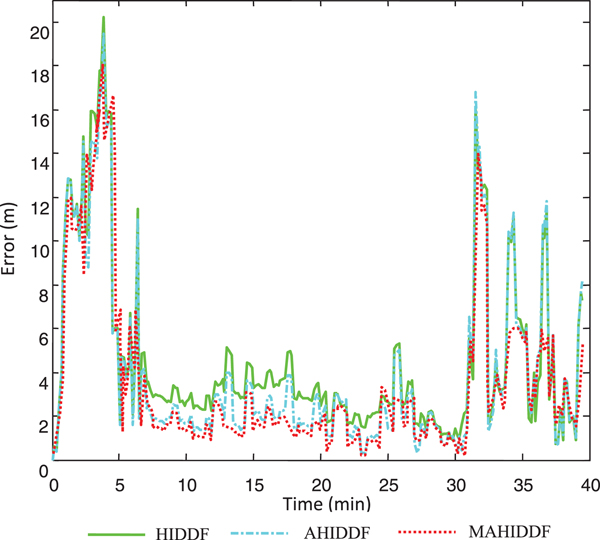
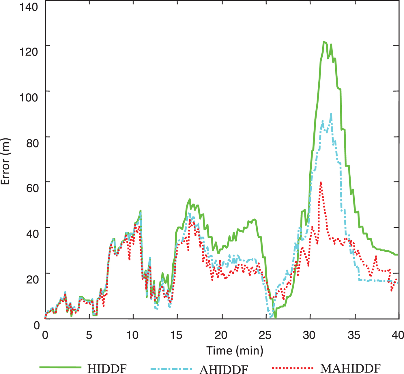
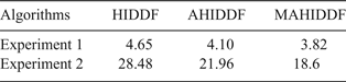
First, performance of the adaptive filtering algorithms under pure Gaussian noise is simulated (ϵ = 0). The simulation results are shown in Figures 2 and 3 for two different trajectories. By comparing the simulation error curves, it can be seen that Huber-based Iterated Divided Difference Filter with weighted Adaptive noise estimation (AHIDDF) and Huber-based Iterated Divided Difference Filter with attenuated Memory Adaptive noise estimation (MAHIDDF) algorithms compensated by noise adaptive estimation have better performance for state estimation compared to the older HIDDF algorithm. Table 1 summarises the cooperative localisation simulation results of different algorithms under Gaussian noise conditions. It can be seen in both the simulation experiments that the newly proposed algorithms have achieved improved performance. The effect is more obvious in Experiment 2.
Comparison of error in Experiment 1 - simulation results under Gaussian noise.

Comparison of error in Experiment 2 - simulation results under Gaussian noise.

Comparison of cooperative positioning error under Gaussian noise simulation (m)

5.2. Simulation under non-noise condition
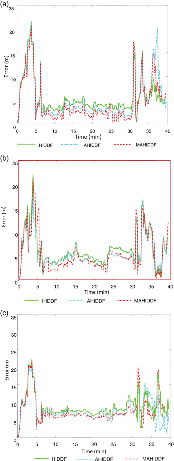
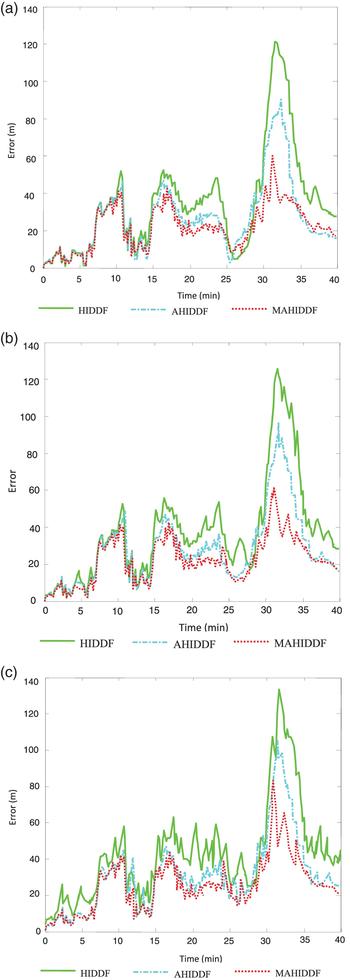
To further verify the robustness of the adaptive filtering algorithm, simulation was also performed under a different non-Gaussian noise condition by setting the value of disturbance coefficient ϵ as 0.1, 0.3 and 0.5. The respective simulation results are shown in Figures 4 and 5 for two different trajectories. It is obvious from the results that with the increase in value of disturbance coefficient, error in state estimation is increased for all the algorithms due to the presence of non-Gaussian noise. However, cooperative localisation performance of the proposed adaptive filters is better than HIDDF in all noise conditions. Simulation error results under non-Gaussian noise condition are summarised in Table 2.
Comparison of error in Experiment 1– simulation results under non-Gaussian noise (a) ε = 0.1 (b) ε = 0.3 (c) ε = 0.5.

Comparison of error in Experiment 2– simulation results under non-Gaussian noise (a) ε = 0.1 (b) ε = 0.3 (c) ε = 0.5.

Comparison of cooperative positioning error under non-Gaussian noise simulation (m)

6. EXPERIMENTAL RESULTS AND ANALYSIS
In order to verify the effectiveness of the proposed algorithm in practical systems, cooperative localisation experiments were conducted in Taihu Lake, Wuxi, China. Then, based on the offline test data, the performance of the algorithm was simulated under dual-pilot and single-pilot vessel schemes. The advantages and feasibility of the proposed algorithm are analysed through performance comparison with different filtering algorithms.
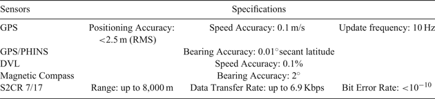
Keeping in mind the complexity of underwater communication and associated system noise characteristics in shallow water, it is sufficient to verify the cooperative localisation performance using surface boats. The pilot/master boats were equipped with a high precision real time Global Positioning System (GPS) system to provide the reference position for cooperative localisation. The slave boat was installed with a DVL and a magnetic compass to estimate its position using Dead Reckoning (DR). To provide a reference base, a GPS / Fog-based High Performance Inertial Navigation System (PHINS) was also installed on the slave boat to provide a relatively accurate position, speed and heading reference. An Evodiaics S2CR 7/17 type acoustics communication system was used for underwater transmission and range measurement. For ease of operation, each master boat sent self-identifier GPS location information and the relative distance measurement information to the slave boat at a fixed interval of 5 s. The slave boat used the dual-master alternative pilot method and no matter from which master boat information was received, it was used for coordinated positioning. Except for the acoustic measurement information, the other sensor information was sampled and processed at intervals of 1 s. The sensor specifications used in the experiment are shown in Table 3.
Specifications of sensors used in Experiments

6.1. Cooperative localisation based on dual-pilot experiment
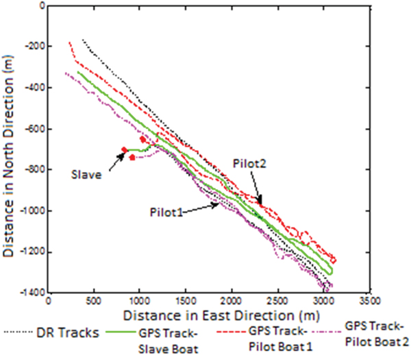
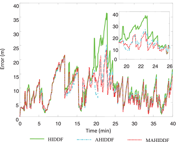
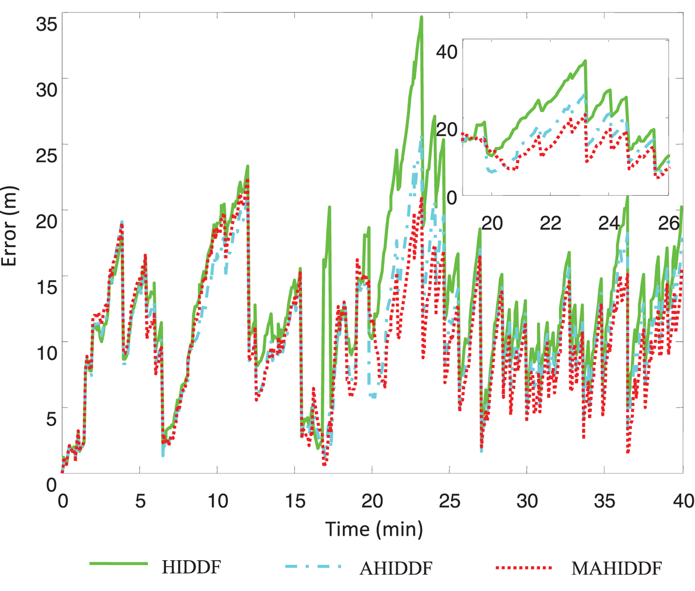
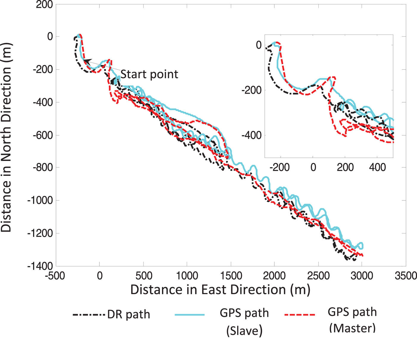
First, a dual pilot experiment was carried out for a cooperative localisation performance test. The average speed of the boats was 2.2 m/s during the experiment. The trajectory of the master-slave boat is shown in Figure 6. A total of 40 experiments were carried out, and intervals of 5 s, 15 s and 30 s were set for offline observation data to verify the cooperative localisation system performance.
Path taken by master and slave boats in dual pilot experiment.

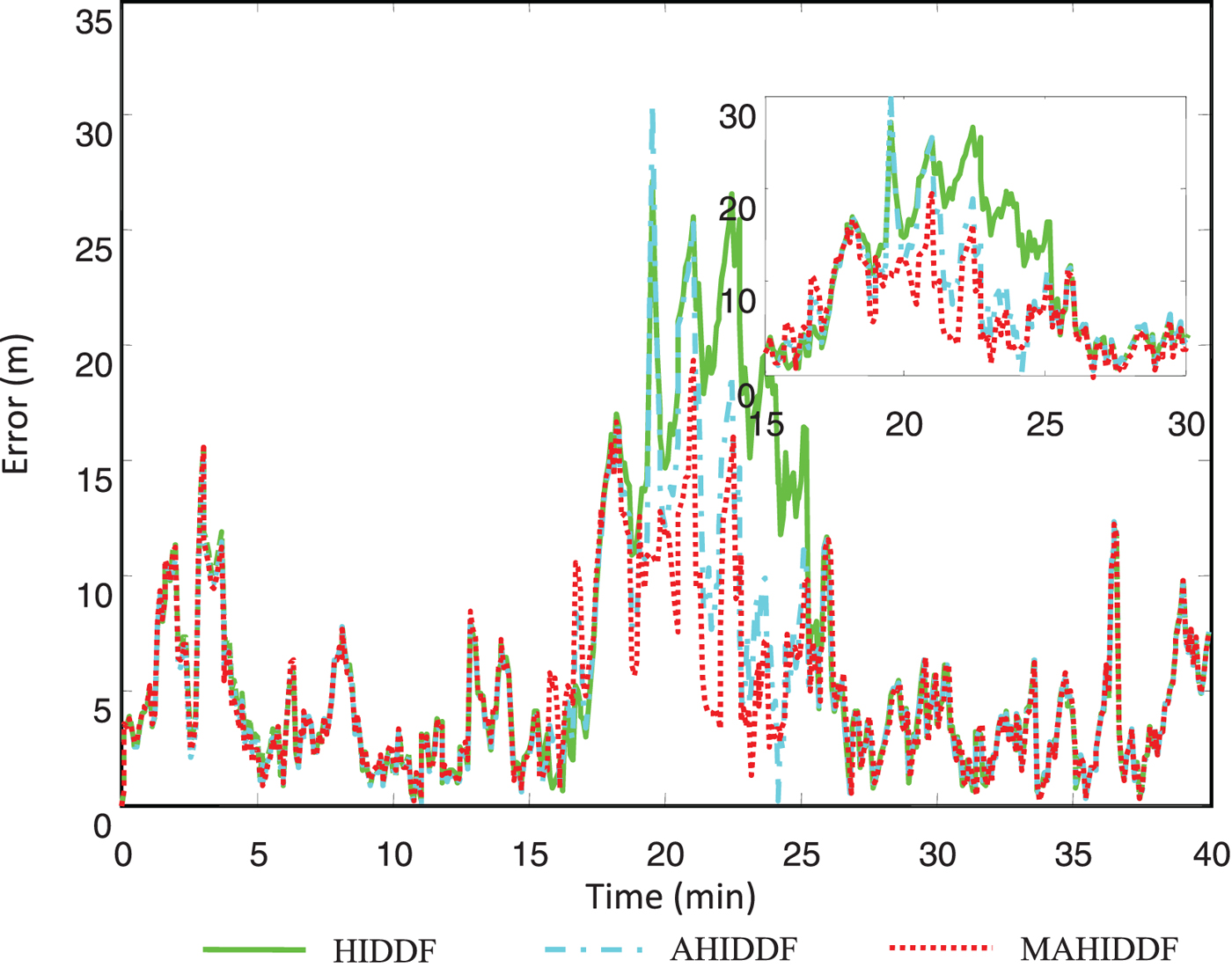
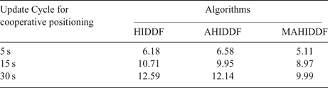
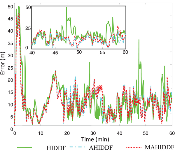
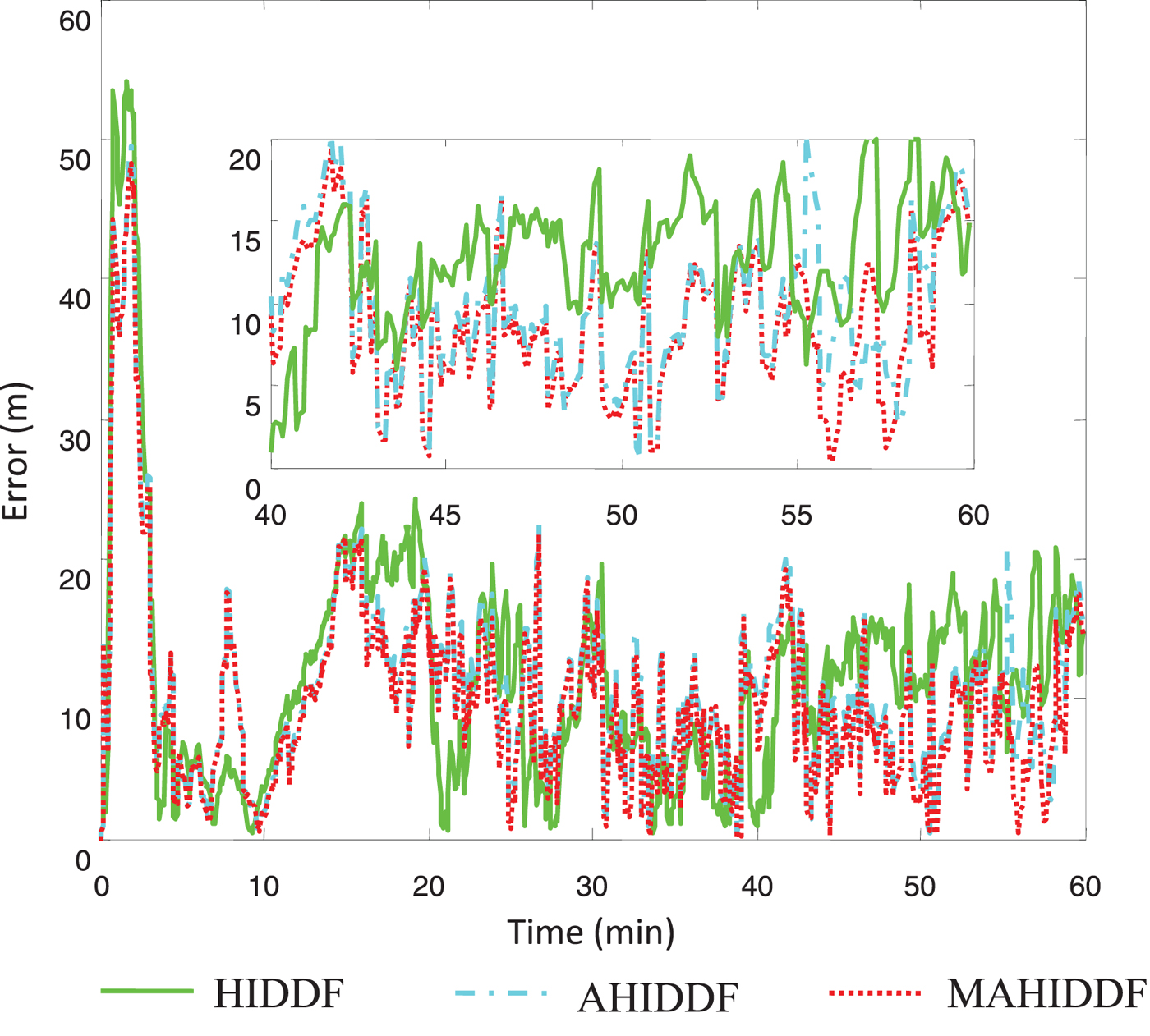
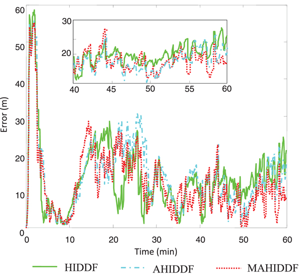
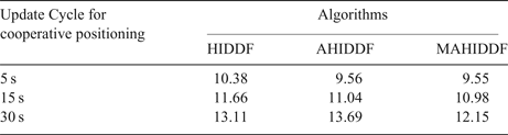
The simulation results based on dual pilot experiment are shown in Figures 7, 8 and 9 for intervals of 5 s, 15 s and 30 s respectively. Analysis of measurement noise indicates that abnormal, heavy tailed noise was observed during the period 18 min–22 min. It can be seen that cooperative localisation based on dual pilot vessel assistance provides timely and effective correction for dead reckoning errors, and the cooperative localisation performance is better. The comparison results indicate that the adaptive filtering algorithm (MAHIDDF), proposed in this paper showed enhanced cooperative localisation performance, especially during the abnormal measurement noise interval at around 20 min. The same is also obvious from the position error results summarised in Table 4. Finally, it is also clear from the results that co-location accuracy also decreases with the extension of the measurement update cycle.
Comparison of position error (5 s update cycle for cooperative localisation).

Comparison of position error (15 s update cycle for cooperative localisation).

Comparison of position error (30 s update cycle for cooperative localisation).

Comparison of cooperative position error for different update cycles (m) - dual pilot experiment

6.2. Cooperative localisation based on single-pilot experiment
In order to test the performance of the proposed algorithm under relatively weak observability conditions, a single pilot experiment was performed. In this experiment, cooperative localisation of one slave boat was performed using updates from a single master boat. The experiment runtime was 1 hr. Based on the offline test data, the algorithm simulations under the cooperative cycles of 5 s, 15 s and 30 s were carried out, respectively. The path taken by master and slave boats is shown in Figure 10.
Path taken by master and slave boats in single pilot experiment.

Analysis of measurement noise for the single pilot experiment indicates that abnormal, heavy tailed noise was observed during a period from 40 min–60 min. The simulation results based on 5 s, 15 s and 30 s cooperative update cycles are shown in Figures 11, 12 and 13, respectively. It can be clearly seen that cooperative localisation performance of all the algorithms has been degraded in the single pilot experiment compared to the dual pilot experiment. This is due to the low observability conditions in the single pilot case compared to the previous case. By comparing the simulation results of different adaptive filtering algorithms, we can see that the adaptive filtering algorithm (MAHIDDF), proposed in this paper, has shown improved performance and position error has remained lower than HIDDF especially during the 40 min-60 min interval. The same is also obvious from the position error results summarised in Table 5.
Comparison of Position Error (5 s update cycle for cooperative localisation).

Comparison of Position Error (15 s update cycle for cooperative localisation).

Comparison of position error (30 s update cycle for cooperative localisation).

Comparison of cooperative position error for different update cycles(m) - single pilot experiment

7. CONCLUSIONS
This paper has presented a weighted adaptive noise estimation filter based on the Myers-Tapley method which is robust against Gaussian as well as non-Gaussian noise. The filter has been used for online noise estimation of AUVs in order to enhance its performance in cooperative localisation. Efficacy of the proposed algorithm has been proved using simulation results as well as practical experiments. Experiments have been conducted using dual-pilot and single-pilot schemes. The results of different cooperative localisation algorithms have been analysed via performance comparison. Both simulation and experiment results show that the proposed method has improved performance especially against abnormal, heavy tailed noise. Future work may include performance comparison of the proposed adaptive noise algorithm with latest adaptive algorithms for cooperative localisation of AUVs.
FINANCIAL SUPPORT
This work was financially supported by key projects of the National Natural Science Fund, No. 61633008, Heilongjiang province post-doctoral research start-up funding project (No. LBHQ15032), and the open funding project of the State Key Laboratory for Marine Engineering (No. 1616).