1. Introduction
Flow around cylindrical-shaped bluff bodies is prevalent in many industrial applications, including high-speed train pantographs, aircraft landing gear struts, bridges and skyscrapers. An important concern in the aerodynamic and hydrodynamic design of such structures is the phenomenon of Kármán vortex shedding, a cyclic vortex formation-shedding process, which occurs beyond the first critical Reynolds number (
 $ \textit{Re}\approx 49$
) (Williamson Reference Williamson1996). This can lead to significant consequences, such as enhanced aerodynamic noise, lift and drag fluctuations, and in turn, vortex-induced vibration. Therefore, controlling, suppressing or ideally eliminating this periodic vortex shedding is highly desirable in such applications.
Current flow control strategies to suppress vortex shedding can be broadly categorised into active and passive approaches (Choi, Jeon & Kim Reference Choi, Jeon and Kim2008). Active approaches, such as plasma actuators (Thomas, Kozlov & Corke Reference Thomas, Kozlov and Corke2008), air blowing and suction (Maryami et al. Reference Maryami, Arcondoulis, Guo and Liu2024a , Reference Maryami, Arcondoulis and Liub ), and synthetic jets (Hu & Morgans Reference Hu and Morgans2023), typically require external energy input. In contrast, passive control methods achieve similar effects via applying local or minimal geometric changes to the objects, e.g. splitter plates (Duan & Wang Reference Duan and Wang2021), porous coatings (Arcondoulis et al. Reference Arcondoulis, Liu, Ragni, Avallone, Rubio-Carpio, Sedaghatizadeh, Yang and Li2023; Maryami et al. Reference Maryami, Arcondoulis, Liu and Liu2023) and local shape modifications. Passive control does not need energy input and is generally simple and cost effective to apply, making it particularly attractive for practical applications. Among various passive control strategies, introducing three-dimensional (3-D) perturbations along the spanwise direction to separated shear layers, known as ‘3-D forcing’ (Choi et al. Reference Choi, Jeon and Kim2008), has proven to be an effective method for both flow and noise control. Typical 3-D forcing control methods include spanwise waviness (Bearman & Owen Reference Bearman and Owen1998; Darekar & Sherwin Reference Darekar and Sherwin2001; Shi et al. Reference Shi, Bai, Alam, Ji and Zhu2023), helical strakes (Korkischko & Meneghini Reference Korkischko and Meneghini2010; Zhou et al. Reference Zhou, Razali, Hao and Cheng2011) and longitudinal grooves (Law & Jaiman Reference Law and Jaiman2018).
For spanwise waviness methods, Lam & Lin (Reference Lam and Lin2008) performed large-eddy simulations (LES) to investigate wavy circular cylinders with wavelength (
 $\lambda _z$
) and diameter (
 $d$
) ratios of
 $1.1\lt \lambda _z/d \lt 3.3$
at
 $ \textit{Re}=3000$
. The optimal wavelength for the best aerodynamic performance was found at
 $\lambda _z = 1.9d$
with a single vortex shedding frequency in the
 $\lambda _z/d$
range considered. Direct numerical simulations (DNS) conducted by Darekar & Sherwin (Reference Darekar and Sherwin2001), on wavy square cylinders with varying
 $\lambda _z$
at
 $ \textit{Re} = 100$
, identified a critical wavelength of
 $\lambda _z =5.6d$
, below which a single vortex shedding frequency was observed, while two distinct shedding frequencies appeared above this critical value. Tombazis & Bearman (Reference Tombazis and Bearman1997) also reported the presence of two vortex shedding frequencies in the wake of wavy blunt trailing edges within
 $3.5 \leqslant \lambda _z/d \leqslant 5.6$
at
 $ \textit{Re} =4\times 10^4$
, and they ascribed the flow control mechanism to vortex dislocations in the wake.
The concept of vortex dislocation was first introduced by Williamson (Reference Williamson1989), who identified two distinct types of coherent vortex structures in the wake behind a circular cylinder with attached end plates, namely the oblique and parallel modes, with distinct vortex shedding frequencies and a phase mismatch. Vortex dislocations can be further categorised into natural and forced dislocations (Williamson Reference Williamson1992). The primary difference between these two categories is that the former is intermittent, occurring during the transition from two-dimensional to 3-D wake structures, and is commonly observed during the wake transition regime, whereas the latter is periodic and typically induced by modifications in geometric configurations, especially sudden spanwise changes such as a cylinder with a ring (Williamson Reference Williamson1992), cylinders with step-change diameter (Morton, Yarusevych & Scarano Reference Morton, Yarusevych and Scarano2016; Massaro, Peplinski & Schlatter Reference Massaro, Peplinski and Schlatter2023; Tian et al. Reference Tian, Zhu, Andersson, Pettersen and Holmedal2025) or twisted finite wings (Pandi & Mittal Reference Pandi and Mittal2023, Reference Pandi and Mittal2025).
Spanwise twisting can be applied to cylinders with a non-circular cross-section, for instance, elliptical cylinders. As an effective method of 3-D forcing, spanwise twisting has a unique advantage over spanwise waviness; namely, its flow control effects are independent on incoming flow direction, which have been explored in several studies on twisted elliptical cylinders. Jung & Yoon (Reference Jung and Yoon2014) performed LES in the subcritical regime (
 $ \textit{Re} = 3000$
), demonstrating excellent flow control capabilities, in terms of maximum reductions of mean drag coefficient
 $\overline {C}_{\kern-1pt D}$
by 13 % and lift coefficient fluctuation
 $C_{\kern-1pt L}'$
by 96 %, along with the optimal aspect ratio (major–minor axis ratio) of
 $1.44$
. The effects of
 $ \textit{Re}$
were further investigated within the subcritical range of
 $3000 \leqslant Re \leqslant 10\,000$
(Yoon, Kim & Kim Reference Yoon, Kim and Kim2019), where the linear increase rate of
 $\overline {C}_{\kern-1pt D}$
and
 $C_{\kern-1pt L}'$
with
 $ \textit{Re}$
was found to be one order of magnitude smaller than that of the straight cylinder. Wei et al. (Reference Wei, Yang, Xia and Li2017) employed cluster-based reduced-order modelling to investigate the wake stabilisation mechanism and identified two distinct wake regimes at
 $ \textit{Re} = 2\times 10^4$
, between which, the in-phase regime exhibited lower
 $\overline {C}_{\kern-1pt D}$
and
 $C_{\kern-1pt L}'$
compared with the antiphase regime. In low
 $ \textit{Re}$
range, the DNS study at
 $ \textit{Re}=100$
by Wei, Yoon & Jung (Reference Wei, Yoon and Jung2016) demonstrated that while the time history of
 $C_{\kern-1pt L}'$
for the twisted cylinder mirrors that of the straight one,
 $C_{\kern-1pt D}$
displays a different pattern due to the formation of 3-D vortical structures along the span. More recently, Yang, Li & Jin (Reference Yang, Li and Jin2024) investigated wake dynamic transition using DNS and identified streamwise vortical structures, i.e. a ‘lock state’ in the spanwise vortex wavelengths, and oblique shedding modes in the wake.
Kim, Lee & Choi (Reference Kim, Lee and Choi2016) introduced spanwise wavelength of
 $2\leqslant \lambda _z/d \leqslant 7$
on top of a helically twisted elliptical cylinder (HTE) using LES, and revealed a maximum drag reduction of 23 % for the case of
 $\lambda _z/d = 4.0$
at
 $ \textit{Re} = 3\,900$
. Inspired by this study, a new geometric modification, referred to as variable pitch HTE, was proposed by Moon & Yoon (Reference Moon and Yoon2020). Their LES performed at
 $ \textit{Re} =3000$
found that
 $C_{\kern-1pt D}$
consistently decreases as pitch increases, with an additional 4.1 % reduction compared with HTE, and that the Strouhal number
 $St$
of vortex shedding,
 $St_{{vs}}$
, becomes lower than that of HTE, suggesting improved wake stability.
Previous studies of twisted cylinders primarily focused on the elliptical cross-section. Polygons, another commonly encountered non-axisymmetric shape, for which spanwise twisting may take similar effects for flow control, have not been considered yet. Even studies on straight polygonal cylinders are scarce. Khaledi & Andersson (Reference Khaledi and Andersson2011) studied the wake behind a hexagonal cylinder (side number
 $N=6$
) in the range of
 $100\leqslant Re \leqslant 1000$
through DNS, and found that the vortex shedding frequency is higher in face orientation (a surface normally facing the incoming flow) than in corner orientation (an edge facing the incoming flow). The aerodynamic performances for polygonal cylinders of
 $N \in \mathbb{Z}[2,16]$
in principal orientations (either face or corner orientation) within
 $10^4\leqslant Re \leqslant 10^5$
were systematically investigated experimentally by Xu et al. (Reference Xu, Zhang, Gan, Li and Zhou2017), who showed that
 $\overline {C}_{\kern-1pt D}$
,
 $C_{\kern-1pt L}'$
and
 $St_{{vs}}$
are all sensitive to
 $N$
and their orientation.
As for the wake flow behind polygonal cylinders, Wang et al. (Reference Wang, Xu, Gan, Zhang and Zhou2019, Reference Wang, Gan, Xu and Zhou2020) conducted particle image velocimetry (PIV) measurements and proper orthogonal decomposition (POD) analysis on the same set of cylinders (
 $N \in \mathbb{Z}[2,16]$
) in their principal orientations in the range of
 $10^4\leqslant Re \leqslant 6\times 10^4$
. Their findings indicated that the effect of side number
 $N$
and orientation on the mean wake flow distribution and vortex patterns can be unified with a properly chosen characteristic length scale. Masoudi et al. (Reference Masoudi, Gan and Sims-Williams2021, Reference Masoudi, Sims-Williams and Gan2023) performed LES studies to explore the shear layer and wake properties of polygonal cylinders of
 $N \in \mathbb{Z}[5,8]$
at arbitrary incidence angles
 $\alpha$
and
 $ \textit{Re}=10^4$
, and found that
 $\alpha$
plays a critical role in determining the wake flow behaviour, attributing to the discretised and periodic distribution of corner-face topology on polygon surface. They also observed that aerodynamic forces and flow separation characteristics exhibit a uniquely non-monotonic behaviour and complex dependencies on both
 $\alpha$
and
 $N$
. Semiempirical equations were derived to predict the separation points on polygonal cylinders and a wake deflection angle was proposed to successfully scale the aerodynamic forces and
 $St_{{vs}}$
. Additionally, a correlation analysis performed by Cheng et al. (Reference Cheng, Masoudi, Liu and Gan2024) revealed that the asymmetric circulation magnitude of the vortices shed on the upper and lower sides of the cylinder, due to the effect of
 $\alpha$
, is responsible for the observed behaviours of
 $\overline {C}_{\kern-1pt D}$
,
 $C_{\kern-1pt L}'$
, and
 $St_{{vs}}$
.
An intriguing finding from the above studies of straight polygonal cylinders across the full range of
 $\alpha$
is that within the group of cylinders
 $N\geqslant 5$
, which have received less attention than square (
 $N=4$
) and triangular (
 $N=3$
) cylinders, the hexagonal cylinder (
 $N=6$
) exhibits distinctive features that deserve special attention. On the one hand,
 $C_{\kern-1pt L}'$
for the hexagonal cylinder can reach notably high values in corner orientation, exceeding those of all other polygonal cylinders and the circular cylinder (Xu et al. Reference Xu, Zhang, Gan, Li and Zhou2017). This suggests the shedding of the most coherent, energetic and symmetric vortex structures from the top and bottom surfaces. On the other hand, at a non-principal orientation, the hexagon exhibits the highest time mean
 $C_{\kern-1pt L}$
, nearly 50 % greater than that of the next highest polygon (observed in the pentagon case), indicating a pronounced asymmetry in vortex shedding strength between the two sides (Masoudi, Gan & Sims-Williams Reference Masoudi, Gan and Sims-Williams2021). These features imply that applying a spanwise twist to the hexagonal cylinder can likely achieve effective flow and noise control, more so than other polygonal cylinders of
 $N\geqslant 5$
, making it a good representative case of passive control strategies for this group of cylinders.
Applying a uniform spanwise twist to a polygonal cylinder introduces a continuous variation in the local incidence angle, resulting in flow characteristics that can differ fundamentally from those observed in twisted elliptical cylinders mentioned above. This difference arises from the potential for local flow reattachment within specific ranges of incidence angles along the span. Moreover, compared with an elliptical cross-section, the polygonal geometry, with its discrete edge–face configuration, could induce stronger flow separation, giving rise to distinct wake dynamics. However, such geometric effects are not necessarily a monotonic function of the twist angle, as will be demonstrated in this study, nor of the number of polygonal sides. Therefore, a systematic investigation of the flow and acoustic characteristics of twisted polygonal cylinders as a passive control strategy represents a valuable contribution to both our fundamental understanding and engineering practice. In this paper, we begin with the case of a twisted hexagonal cylinder.
In the present study, we adopt a combined systematic experimental and numerical approach to demonstrate this control effect. Far-field noise is measured for flow over hexagonal cylinders with varying twist angles to identify the geometry that results in the best noise reduction effect. Subsequently, wall-resolved LES simulations are performed to reveal the underlying mechanisms. Section 2 describes the noise measurement set-up, and § 3 outlines the numerical method. The main findings, including the spanwise variation of flow separation and the resultant wake properties are presented in § 4. The primary mechanisms of flow and noise control are discussed in § 4.6. Finally, the conclusions are drawn in § 5.
2. Experimental set-up
2.1. Cylinder geometry
The geometry of the twisted hexagonal cylinder employed in the experiment is shown in figure 1. The inscribed circle diameter of the hexagonal cross-section,
 $D_i = 25$
mm, is used to define the Reynolds number
 $ \textit{Re}$
along with the incoming free stream velocity
 $U_\infty$
. A twist angle
 $\phi _0 = \pi /3$
is uniformly applied over a span
 $L_s$
, which defines the twist wavelength, so that the two end surfaces over
 $L_s$
have the identical orientation, i.e.
 \begin{align} \phi (z)=\phi _0 \big[(z-z_0)/L_s \big], \end{align}
where
 $z_0$
is at the cylinder midspan, as depicted in figure 1(
 $b$
), and
 $\phi (z_0)=0$
. To differentiate from the wavelength for wavy cylinders, which is commonly denoted as
 $\lambda _z$
, here
 $L_s$
is used for the twist wavelength, which is also the span for the LES simulations described in § 3. The degree of twisting is defined by twist angle per unit span as
 \begin{align} \gamma ^* = \phi _0\left (\frac {D_i}{L_s}\right ) \!. \end{align}
(
 $a$
) Schematic of the far-field noise experimental set-up with a twisted cylinder placed in an aeroacoustic wind tunnel. (
 $b$
) Isometric view of the twisted cylinder. (
 $c$
) Midspan sectional view in the corner orientation, where
 $\pm \theta$
label the positive and negative azimuthal directions.

As summarised in table 1, a straight cylinder and 10 twisted cylinders with increasing
 $\gamma ^*$
were experimentally investigated. These cylinders were mounted in the wind tunnel to satisfy the corner orientation condition at the cylinder midspan
 $z=z_0$
, i.e. the incidence angle
 $\theta _0=0^\circ$
, unless stated otherwise. All cylinders have a constant 550 mm total span, resulting in an aspect ratio of 22, as shown in figure 1(
 $b$
). Consequently, cases with increasing
 $\gamma ^*$
have a larger number of twist wavelengths covered within the total cylinder span. The effect of this inconsistency on noise radiation is negligible, since the primary contribution to the measured far-field noise arises from the span length due to the low spanwise coherence, as will be discussed in § 4.3. The lowest achievable
 $\gamma ^*$
,
 $1/18$
, corresponding to
 $L_s=6\pi D_i$
, is limited by the size of the wind tunnel, which accommodates slightly more than one
 $L_s$
. The test models were fabricated using photosensitive resin 3-D light-curing printing technology, finely ground to minimise surface roughness and the tendency of premature transition of the laminar boundary layer before flow separation.
Tested cases with varying unit span twist angle
 $\gamma ^*$
. The LES simulations are performed for the four cases (Cases 0, 4, 7 and 10) marked with
 $\dagger$
.

2.2. Acoustic measurements
Far-field noise measurements were conducted in a low-speed, open-jet anechoic wind tunnel at the Southern University of Science and Technology (SUSTech), as shown in figure 1(
 $a$
), at free stream velocities
 $U_\infty$
ranging from 12
 $\mathrm{m\,s}^{-1}$
to 60
 $\mathrm{m\,s}^{-1}$
with a 6
 $\mathrm{m\,s}^{-1}$
interval, corresponding to the testing
 $ \textit{Re}$
range of
 $2\times 10^4$
–
 $10^5$
. The test section has a cross-sectional area of 0.6 m
 $\times$
0.55 m. The inner dimensions of the anechoic chamber are 3.8 m
 $\times$
5.7 m
 $\times$
3.0 m, with the cutoff frequency of 100 Hz for a 1.9 m free-field radius. The wind speed in the open test section can reach up to 70
 $\mathrm{m\,s}^{-1}$
with the turbulence level lower than 0.15 % at
 $U_\infty =50$
 $\mathrm{m\,s}^{-1}$
. More details of the SUSTech anechoic wind tunnel can be found in Yang et al. (Reference Yang, Liu, Liu, Shen, Zhang, Wei, Liu and Xu2021).
A Brüel & Kjær 4966-H-041 far-field microphone was positioned 1.5 m horizontally from the midspan of the vertically mounted model in the test section. Acoustic data were collected using an NI PXI-10,420 chassis and a 24-bit NI PXI-4496 data acquisition card, with a sampling frequency of 51.2 kHz (
 $St=fD_i/U_{\infty }\approx 1066.7$
) and a sampling duration of 20 s. Acoustic pressure signals were then transformed into power spectral density (PSD),
 $\phi _{pp}$
, using Welch’s method. The dataset was partitioned into 160 segments with a 50 % overlap for averaging, resulting in a resolution of 2 Hz (
 $St\approx 0.0042$
). The far-field acoustic PSD in
 $\mathrm{dB\,Hz}^{-1}$
was obtained as follows:
 \begin{align} \varPhi _{pp}=10\log _{10} \left (\frac {\phi _{\mathit{pp}}}{p^2_{\textit{ref}}} \right ) \!, \end{align}
where the reference pressure
 $p_{\textit{ref}} = 2 \times 10^{-5}$
Pa.
3. Numerical methodology
3.1. Governing equations and numerical schemes
To resolve the flow around the twisted hexagonal cylinder in this
 $ \textit{Re}$
range, which is plausibly highly 3-D and unsteady, LES simulations were conducted aiming to solve the unsteady Navier–Stokes equation by segregating large- and small-scale vortices by applying an implicit low-pass filtering. The unsteady and spatially filtered incompressible governing equations are written as
 \begin{align} \frac {\partial \tilde {u}_i}{\partial x_i}=0, \\[-28pt] \nonumber \end{align}
 \begin{align} \frac {\partial \tilde {u}_i}{\partial t}+\frac {\partial \tilde {u}_i\tilde {u}_{\kern-1pt j}}{\partial x_{\kern-1pt j}}=-\frac {1}{\rho }\frac {\partial \tilde {p}}{\partial x_i}+\frac {\partial }{\partial x_{\kern-1pt j}}\left [\nu \left (\frac {\partial \tilde {u}_i}{\partial x_{\kern-1pt j}}+\frac {\partial \tilde {u}_{\kern-1pt j}}{\partial x_i}\right )+\tau _{\textit{ij}}\right ], \\[-2pt] \nonumber \end{align}
where
 $x_i$
represents the Cartesian coordinates,
 $\tilde {u}$
and
 $\tilde {p}$
are the spatially filtered velocity and pressure, and
 $\tau _{\textit{ij}}$
denotes the viscous stress tensor.
The subgrid-scale (SGS) stress tensor is given by
 $\tau _{\textit{ij}}=\widetilde {u_i u_{\kern-1pt j}}-\tilde {u}_i \tilde {u}_{\kern-1pt j}$
, which represents the momentum transport between filtered flow field and unresolved SGS turbulence, and was modelled to close the filtered continuity and momentum equations. Wall-adapting local eddy-viscosity model (Nicoud & Ducros Reference Nicoud and Ducros1999) based on an eddy-viscosity assumption was used in the present study, which demonstrates a good capability of capturing the near-wall flow field,
 \begin{align} \tau _{\textit{ij}} - \frac {1}{3}\tau _{kk}\delta _{\textit{ij}}=2\nu _t\tilde {S}_{\textit{ij}}, \end{align}
where
 $\tilde {S}_{\textit{ij}}$
is the rate of strain tensor defined as
 $\tilde {S}_{\textit{ij}}=1/2 (\tilde {g}_{\textit{ij}} + \tilde {g}_{\textit{ji}} )$
with the velocity gradient tensor
 $\tilde {g}_{\textit{ij}} = \partial \tilde {u}_i/\partial x_{\kern-1pt j}$
, and
 $\nu _{t}$
denotes the SGS viscosity defined as
 \begin{align} \nu _t = (C_w\varDelta )^2\frac {\big(S^d_{\textit{ij}} S^d_{\textit{ij}} \big)^{3/2}}{\big(\tilde {S}_{\textit{ij}}\tilde {S}_{\textit{ij}} \big)^{5/2}+ \big(S^d_{\textit{ij}} S^d_{\textit{ij}} \big)^{5/4}} , \end{align}
where
 $C_w = 0.325$
is the model coefficient,
 $\varDelta$
the filtration scale and
 $S^d_{\textit{ij}}$
the traceless symmetric part of the velocity gradient tensor square,
 \begin{align} S^d_{\textit{ij}} = \frac {1}{2}\big (\tilde {g}_{\textit{ij}}^2 + \tilde {g}_{\textit{ji}}^2\big ) - \frac {1}{3}\delta _{\textit{ij}} \tilde {g}_{kk}^2. \end{align}
The simulations were implemented in OpenFOAM. The Gauss linear scheme was used for pressure and velocity gradient discretisation, and the divergence term was discretised by a linear-upwind stabilised transport scheme, which combines linear upwind and linear interpolation with weighting factors 0.25 and 0.75 to stabilise the solutions. The implicit three-level scheme (backward) was applied for time stepping. A pressure-implicit with split-operator algorithm (Patankar & Spalding Reference Patankar and Spalding1983) was applied to couple pressure and velocity. The generalised geometric–algebraic multigrid numerical solver was set for pressure, and the smooth solver was used for velocity. Three pressure-implicit with split-operator correctors were used for each time step to obtain the final results. A dynamic time step was utilised to ensure that the maximum Courant number
 $Co=U_{\infty }\Delta t/\Delta x \leqslant 1$
. Statistical flow field data were sampled for a duration of 0.4 s which corresponds to at least 30 complete vortex shedding cycles after a quasisteady state was reached for all cases.
In the present study, far-field noise was predicted using the Ffowcs Williams–Hawkings (FW–H) equation with the Farassat 1A formulation (Brentner & Farassat Reference Brentner and Farassat1998). Built upon the foundational works of Lighthill (Reference Lighthill1952) and Curle (Reference Curle1955), the FW–H equation (Williams & Hawkings Reference Williams and Hawkings1969) is written as
 \begin{align} \left (\frac {\partial ^2}{\partial t^2} - c_0^2 {\nabla} ^2\right ) \big [H(f) \rho '\big ] & = \frac {\partial ^2}{\partial x_i \partial x_{\kern-1pt j}} \big [T_{\textit{ij}} H(f)\big ] \nonumber \\& \quad + \frac {\partial }{\partial t} \big [\rho _0 v_n + \rho (u_n - v_n) \delta (f)\big ] \nonumber \\& \quad - \frac {\partial }{\partial x_i} \left \{\big [p_{\textit{ij}} n_{\kern-1pt j} + \rho u_i (u_n - v_n)\big ] \delta (f) \right \}, \end{align}
which is an inhomogeneous wave equation, with the right-hand side comprising three types of acoustic sources in order, i.e. the quadrupole, monopole and dipole terms. The quadrupole term, associated with turbulence in the flow field, is represented by the Lighthill stress tensor
 $T_{\textit{ij}} = \rho u_i u_{\kern-1pt j} + p_{\textit{ij}} - c_0^2 \rho '\delta _{\textit{ij}}$
. The monopole term corresponds to unsteady mass flux, and the dipole term is due to unsteady forces applied on the body surface. In (3.6),
 $H(f)$
is the Heaviside function;
 $\rho _0, c_0$
denote the density and speed of sound in ambient air, respectively, and
 $\rho '$
the fluid density fluctuation; the term
 $u_i$
represents the surface velocity component in the
 $i$
-direction, while
 $u_n$
and
 $v_n$
are the normal components of the fluid and surface velocities, respectively, with
 $n_{\kern-1pt j}$
the surface normal vector;
 $p_{\textit{ij}} = p'\delta _{\textit{ij}}-\tau _{\textit{ij}}$
denotes the compressive stress tensor with
 $p'$
the pressure fluctuation. For flow around stationary bluff bodies at low Mach numbers (
 $Ma \lt 0.3$
), as in the case of this study, quadrupole noise is negligible and the monopole term vanishes over the surface, thus leaving the dipole term the dominant acoustic source. For the calculation of far-field noise, a dynamic library libAcoustics developed by Epikhin et al. (Reference Epikhin, Evdokimov, Kraposhin, Kalugin and Strijhak2015) was used in the present study. The FW–H impermeable integration surface is placed on cylinders. The far-field receiver is placed in the midspan plane at a constant radius of
 $R=60D_i$
, which is the same as the experimental set-up.
3.2. Computational domain and boundary conditions
An O-shaped computational domain of diameter
 $40D_i$
was adopted as illustrated in figure 2. The cylinder was positioned at the domain centre, whose spanwise length was set to be the twist wavelength
 $L_s$
, so that periodic boundary conditions can be applied at the two end surfaces of the domain. Following the experimental set-up in § 2.1, the corner orientation was also achieved at the cylinder midspan (i.e.
 $z_0/L_s=0.5$
). The absolute span of the cylinder therefore varies according to the
 $\gamma ^*$
value and (2.2). For the straight cylinder with
 $\gamma ^*=0$
,
 $L_s$
was set to be
 $\pi D_i$
(Masoudi, Sims-Williams & Gan Reference Masoudi, Sims-Williams and Gan2023). The domain size provides satisfactory accuracy for similar LES tasks under comparable
 $ \textit{Re}$
conditions (Kravchenko & Moin Reference Kravchenko and Moin2000; Cheng et al. Reference Cheng, Pullin, Samtaney, Zhang and Gao2017; Masoudi et al. Reference Masoudi, Gan and Sims-Williams2021). Over the inlet surface, the Dirichlet boundary condition,
 $\boldsymbol {U} = (U_{\infty },0,0)$
, was applied with zero pressure gradient (
 $\partial p/\partial n = 0$
). At the outlet, Neumann boundary condition was applied to the velocity, and the pressure was set to zero (Jiang et al. Reference Jiang, Hu, Cheng and Zhou2022; Zhang et al. Reference Zhang, Kareem, Xu and Jiang2023). A standard no-slip boundary condition was applied to the cylinder surface.
Schematic of the computational domain and boundary conditions: (
 $a$
) isometric view; (
 $b$
) top view; (
 $c$
) side view.

(
 $a$
) Structured hexahedral grid shown in the
 $x$
–
 $y$
plane. (
 $b$
) Histogram of the grid cell count for the LES resolution
 $M$
.

The present LES study utilised structured hexahedral grids, which extend outward from the cylinder surface with a growth rate of 1.1 in the
 $x$
–
 $y$
plane, see figure 3(
 $a$
). The first layer was positioned at a distance of
 $y/D_i=4\times 10^{-4}$
from the cylinder surface, ensuring
 $y^+\lt 1$
. In the present work, the drag coefficient
 $C_{\kern-1pt D}$
, lift coefficient
 $C_{\kern-1pt L}$
and Strouhal number
 $St_0$
of dominant vortex shedding are defined as
 \begin{align} C_{\kern-1pt D}=\frac {F_D}{0.5\rho U^2_{\infty } (L_s D_i)}, \qquad C_{\kern-1pt L}=\frac {F_L}{0.5\rho U^2_{\infty } (L_s D_i)}, \\[-28pt] \nonumber \end{align}
 \begin{align} St_0=\frac {f_0D_i}{U_\infty }, \\[-2pt] \nonumber \end{align}
where
 $F_D$
and
 $F_L$
are the drag and lift forces, respectively, and
 $f_0$
represents the predominant tonal frequency determined from the far-field noise PSD. The time-averaged
 $\overline {C}_{\kern-1pt D}$
and
 $St_0$
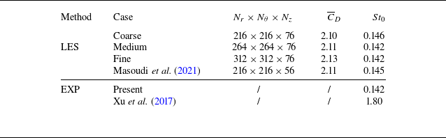
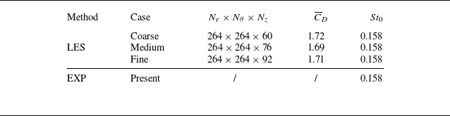
were used for the grid sensitivity analysis, with further details provided in Appendix A.
The final adopted mesh consists of 264 grid points in both radial (
 $r$
) and azimuthal (
 $\theta$
) directions and 76 grid points uniformly distributed in the spanwise
 $z$
-direction for
 $\gamma ^* = 0$
and
 $1/3$
(152 and 228 grid points for
 $\gamma ^* = 1/6$
and
 $1/9$
, respectively). The LES spatial resolution was evaluated by the ratio of the resolved turbulence kinetic energy (TKE), denoted as
 $k_{\textit{res}}$
, to the overall TKE, which is the sum of
 $k_{\textit{res}}$
and the subgrid TKE,
 $k_{\textit{sgs}}$
, i.e.
 \begin{align} M = \frac {k_{\textit{res}}}{k_{\textit{sgs}}+k_{\textit{res}}}, \end{align}
where the ratio
 $M$
was calculated from over 30 vortex shedding cycles. Accurate LES requires sufficiently fine grids to resolve 80 % of TKE (Pope Reference Pope2001). The histogram of
 $M$
for Case 10 (
 $\gamma ^* = 1/3$
), which has the strongest twist (see table 1), is presented in figure 3(
 $b$
). It indicates that approximately 94 % of the mesh cell counts resolve more than 90 % of the TKE. Therefore, the adopted grid with the chosen scheme is considered reasonably accurate for the flow field quantities under investigation. The current numerical scheme was also validated by comparing the time-averaged streamwise velocity distribution over the
 $x$
–
 $z$
plane at
 $y=0$
, with that obtained from a PIV experiment. More details can be found in Appendix B.
In addition to the straight cylinder (
 $\gamma ^*=0$
), three twist cases of
 $\gamma ^* = 1/9$
,
 $1/6$
and
 $1/3$
, representing a weak, optimal and strong twist, respectively, were selected for detailed LES simulations (see table 1), matching the lower
 $ \textit{Re}$
bound of the experiment at
 $ \textit{Re}=2\times 10^4$
. An spanwise correction method for acoustic prediction proposed by Kato et al. (Reference Kato, Iida, Takano, Fujita and Ikegawa1993), which is shown in Appendix C, was adopted to account for the discrepancy in cylinder lengths between the simulation and the experiment, facilitating a cross-comparison. Figure 4 shows that the corrected far-field noise PSD spectra are in good agreement with the measured data for
 $\gamma ^* = 0$
(the straight cylinder) and
 $\gamma ^* = 1/3$
(the most twisted case). The case
 $\gamma ^* = 1/6$
with the optimal control effect, which will be demonstrated in § 4, is also shown, but the agreement is worse. This is attributed to the unique wake characteristics of this case, as will be examined and presented in § 4.3, which cannot be fully captured by LES within reasonable simulation time.
Comparison of far-field noise PSD between numerical simulations (corrected) and experiments at
 $ \textit{Re} = 2 \times 10^4$
: (a)
 $\gamma ^* = 0$
and
 $1/9$
; (b)
 $\gamma ^* = 1/6$
and
 $1/3$
. The cases of
 $\gamma ^*=0$
and
 $1/3$
are shifted in the vertical direction for better visualisation.

3.3. Proper orthogonal decomposition
In the present study, a snapshot-based POD proposed by Sirovich (Reference Sirovich1987) was employed to evaluate flow structure coherency for the 3-D velocity field obtained from LES. Simulated flow velocity data were linearly interpolated to uniform rectilinear coordinates
 $\boldsymbol{x}$
, such that each vector in a snapshot
 $\boldsymbol{q}(\boldsymbol{x}, t)$
is written in a structure
 \begin{align} \boldsymbol{q}(\boldsymbol{x}, t) = [u(\boldsymbol{x}, t),v(\boldsymbol{x}, t),w(\boldsymbol{x}, t)]^T, \end{align}
where
 $t$
is the discrete time;
 $u$
,
 $v$
and
 $w$
are the velocity components in the
 $x$
-,
 $y$
- and
 $z$
-axes, respectively;
 $\boldsymbol{q}(\boldsymbol{x}, t)$
is a concatenated vector for the three velocity components with dimension
 $3N$
, where
 $N$
is the number of grid points in a snapshot. The
 $K$
snapshots are then assembled into a matrix as
 \begin{align} \boldsymbol{Q} = \begin{bmatrix} \boldsymbol{q'}(\boldsymbol{x}, t_1) & \boldsymbol{q'}(\boldsymbol{x}, t_2) & {\cdots} & \boldsymbol{q'}(\boldsymbol{x}, t_M) \end{bmatrix} \in \mathbb{R}^{3N \times K} , \end{align}
where
 $\boldsymbol{q'}(\boldsymbol{x}, t) = \boldsymbol{q}(\boldsymbol{x}, t) - \boldsymbol{\overline {q}}(\boldsymbol{x})$
, with
 $\boldsymbol{\overline {q}}(\boldsymbol{x})$
the time-averaged quantity.
The covariance matrix
 $\boldsymbol{C} = \boldsymbol{Q^T Q}$
is then constructed for an eigenvalue problem,
 \begin{align} \boldsymbol{C} \psi _j = \lambda _j \psi _j, \end{align}
where
 $\psi _j$
is the
 $j$
th eigenvector. The
 $j$
th POD mode can be calculated as
 \begin{align} \phi _j = \boldsymbol{Q} \psi _j \frac {{1}}{\sqrt {\lambda _j}}. \end{align}
These modes are orthogonal and ranked according to their energy content which is the eigenvalue
 $\lambda$
. The instantaneous velocity field can be ‘smoothed’ by a truncated expansion using the leading
 $r$
(
 $r\leqslant M$
) POD modes,
 \begin{align} \boldsymbol{q}(\boldsymbol{x}, t) \approx \boldsymbol{\overline {q}}(\boldsymbol{x})+\sum _{j=1}^{r} a_j(t) \phi _j(\boldsymbol{x}), \end{align}
where
 $a_j(t)$
is the POD coefficient corresponding to the
 $j$
th mode, computed by projecting the flow field fluctuation onto the POD modes as
 \begin{align} \boldsymbol{a}(t) = [\phi _1,\phi _2,\ldots ,\phi _K]^T \boldsymbol{q}'(\boldsymbol{x}, t) \in R^{K\times 1}. \end{align}
A total of 2000 snapshots were extracted evenly distributed over the sampling time duration of 0.4 s, corresponding to at least 30 vortex shedding cycles. A convergence test was conducted, confirming that 30 cycles were sufficient to achieve satisfactory statistical convergence. The POD was performed over the ‘whole’ wake volume, and also regional volumes, as will be presented in § 4.3.
4. Results and discussion
4.1. Aeroacoustic and aerodynamic characteristics
Far-field noise PSD,
 $\varPhi _{pp}$
(dB Hz−1), derived from the experimental noise data according to (2.3), is presented in figure 5(
 $a$
), which demonstrates a dominant peak occurring at
 $St = 0.142$
for the straight corner-oriented hexagonal cylinder (the baseline case
 $\gamma ^* = 0$
). This corresponds to the fundamental Kármán vortex shedding from the straight cylinder as defined in (3.7b
), hereafter denoted as
 $St_0$
, which agrees well with previous LES (Masoudi et al. Reference Masoudi, Gan and Sims-Williams2021) and experimental (Xu et al. Reference Xu, Zhang, Gan, Li and Zhou2017) studies. When twisting is introduced, all
 $\gamma ^* \gt 0$
cases are shown to reduce both the tonal and broadband noise levels relative to the baseline, where the case
 $\gamma ^* = 1/6$
demonstrates a remarkable tonal noise reduction of up to 15 dB. A noteworthy observation is that for the cases displaying a single dominant peak,
 $\varPhi _{pp}$
is not a monotonic function of
 $\gamma ^*$
, i.e.
 $\varPhi _{pp}|_{\gamma ^*=0}\gt \varPhi _{pp}|_{\gamma ^*=1/3}\gt \varPhi _{pp}|_{\gamma ^*=1/6}$
.
(
 $a$
) Far-field noise PSD,
 $\varPhi _{pp}$
, for varying
 $\gamma ^*$
cases. (
 $b$
) Dependence of the number of tones on
 $\gamma ^*$
, where the marker size is proportional to the peak
 $\varPhi _{pp}$
value. Experimental data at
 $ \textit{Re} = 2\times 10^4$
.

Another interesting observation is the change of the number of tones in the noise spectrum as
 $\gamma ^*$
increases. The tone number increases from one for the baseline case (
 $\gamma ^*=0$
) to two as
 $\gamma ^*$
reaches
 $1/18$
, and then remains at two until
 $\gamma ^*\lesssim 1/6$
, beyond which the spectrum reduces back to a single tone at
 $St_0$
, larger than that of the baseline yet with lower
 $\varPhi _{pp}$
. The dual tone observed within
 $1/18\leqslant \gamma ^*\lesssim 1/6$
suggests a vortex shedding pattern deviating from the classical Kármán type, which is plausibly attributed to spatial variation of spanwise twist, rather than to a temporal switch of vortex-shedding modes. These two patterns are labelled as Patterns I and II, respectively, as shown in figure 5(
 $b$
), which will be elaborated in § 4.3. The frequencies for the two tones in this
 $\gamma ^*$
range are denoted as
 $St_1$
and
 $St_2$
, respectively. Exactly at which
 $\gamma ^*$
the second tone starts to emerge in the range
 $0\lt \gamma ^*\lt 1/18$
cannot be convincingly determined from the experiments due to the spatial constraint of the wind tunnel as explained in § 2. A close inspection of the inset plot in figure 5(
 $a$
) reveals that the spectrum for the case
 $\gamma ^* = 1/6$
appears to lie between the single-tone and dual-tone cases. It can be interpreted either as a single, blunt hump or as two peaks without a clearly defined valley between them. This feature, as will be shown later, leads to a promising simultaneous noise reduction effect (aeroacoustically) and a stabilising effect (aerodynamically), with the optimal performance apparently occurring near
 $\gamma ^* = 1/6$
.
Twisted cylinders can be viewed as cylinders whose given cross-sectional shape (a hexagon in this case) rotates in the same direction along the span with an infinitesimal step, resulting in a continuously changing sectional incidence
 $\phi (z)$
and, in turn, a varying sectional flow separation point. Masoudi et al. (Reference Masoudi, Gan and Sims-Williams2021) found that for the straight hexagonal cylinder the vortex shedding frequency varies smoothly in the range
 $0.14\lesssim St_0 \lesssim 0.17$
as the incidence angle changes. When twist is applied,
 $St_1$
and
 $St_2$
in Pattern II likely originate from a similar range of incidence angles. In this regime, the corresponding frequencies exhibit a bimodal distribution centred around two preferred values of
 $St_1 \approx 0.14$
and
 $St_2 \approx 0.17$
, rather than a broadband spectrum. As the degree of twist further increases to
 $\gamma ^*\geqslant 1/5.4$
, only one preferred frequency is selected, which is
 $St_0$
in Pattern I, with its value (
 $\approx 0.16$
) almost equivalent to the arithmetic mean of
 $St_0$
(
 $\approx 0.157$
) across all incidence angles of a straight hexagonal cylinder.
The total far-field noise was evaluated by integrating the PSD
 $\varPhi _{pp}$
over
 $ 0.1\lesssim St\lesssim 5$
, yielding the OASPL. The effect of spanwise twist on noise reduction with respect to the baseline case (
 $\Delta$
OASPL) is obvious, as shown in figure 6(
 $a$
). The nonlinearly varying
 $\Delta$
OASPL with
 $\gamma ^*$
minimises at
 $\gamma ^* = 1/6$
, achieving a total noise reduction increasing with
 $ \textit{Re}$
, viz., 11 dB at
 $ \textit{Re}=2\times 10^4$
and 17 dB at
 $ \textit{Re}=10^5$
. In addition, the dependence of OASPL on the cylinder orientation, measured by the midspan incidence
 $\theta _0$
, is much weaker than on the twist angle, which is demonstrated in figure 7. As shown in figure 6(
 $b$
), the far-field acoustic radiation exhibits a consistent scaling with the
 $Ma^6$
law regardless of
 $\gamma ^*$
, a characteristic of dipole sound sources, suggesting that the unsteady forces on the cylinder surface are the primary noise source. Within the tested subcritical
 $ \textit{Re}$
range, the case with
 $\gamma ^* = 1/6$
consistently shows the best noise reduction performance, underscoring the potential practical value of this specific twist angle.
(
 $a$
) Dependence of measured overall sound pressure level (OASPL) reduction on
 $\gamma ^*$
at
 $ \textit{Re} = 2\times 10^4$
,
 $6\times 10^4$
and
 $1\times 10^5$
. (
 $b$
) Variation of OASPL with Reynolds number for varying
 $\gamma ^*$
cases.

Variation of far-field OASPL with cylinder midspan incidence angle
 $\theta _0$
and
 $\gamma ^*$
. Experimental data at
 $ \textit{Re} = 2\times 10^4$
.

Comparison of aerodynamic performance for the twisted and straight cylinders at
 $ \textit{Re} = 2\times 10^4$
, obtained from numerical simulations. (
 $a$
,
 $b$
) Time history of drag and lift coefficients, (
 $c$
) phase-space plot of the force coefficients, (
 $d$
) PSD of lift coefficient fluctuation.

The far-field OASPL is associated with the flow field whose global characteristics can be captured by the time history of
 $C_{\kern-1pt D}$
and
 $C_{\kern-1pt L}$
, as shown in figure 8(
 $a$
,
 $b$
), where
 $t^*=tU_\infty /D_i$
. These simulation results suggest that their fluctuation level, e.g. the root-mean-square (r.m.s.) values calculated based on 30 shedding cycles, namely
 $C'_{L,\textit{rms}}$
and
 $C'_{D,\textit{rms}}$
, as well as the time-averaged drag,
 $\overline {C}_{\kern-1pt D}$
, are significantly reduced for twisted cylinders, perhaps as expected. In line with the noise spectrum is the non-monotonic variation of the fluid forces with increasing
 $\gamma ^*$
. To facilitate a clear comparison of their features in time domain, figure 8(
 $c$
) shows the phase diagram, where the strongest suppression of the oscillation amplitude of the two fluid forces for the
 $\gamma ^* = 1/6$
case is evident. In particular,
 $C'_{L,\textit{rms}}$
,
 $C'_{D,\textit{rms}}$
and
 $\overline {C}_{\kern-1pt D}$
are reduced by 90 %, 27 % and 37 %, respectively, compared with the baseline case. The
 $\overline {C}_{\kern-1pt D}$
value is also lower than that of the straight hexagonal cylinder in any orientation, which is typically
 $\gtrsim 1.5$
under a similar subcritical
 $ \textit{Re}$
(Masoudi et al. Reference Masoudi, Gan and Sims-Williams2021).
The PSD of
 $C_{\kern-1pt L}'$
for the four cases are shown in figure 8(
 $d$
), with the
 $\gamma ^* = 1/6$
case exhibiting the lowest dominant spectral peak. This supports the finding of the most significant far-field noise attenuation for this case, as shown in figure 6(
 $a$
), since the dominant acoustic radiation perpendicular to the free stream is associated with the fundamental frequency of lift fluctuations in a dipole source (Gerrard Reference Gerrard1955; Etkin, Korbacher & Keefe Reference Etkin, Korbacher and Keefe1957). Consistent with the behaviour of
 $\varPhi _{pp}$
, the case with
 $\gamma ^* = 1/9$
displays two distinct peaks, reinforcing the link between the near-field flow dynamics and far-field noise.
The aerodynamic and aeroacoustic results presented in this section therefore suggest that the twist angle
 $\gamma ^* = 1/6$
somehow yields the optimal control effect on a hexagonal cylinder, which minimises the tonal peak, OASPL,
 $\overline {C}_{\kern-1pt D}$
and r.m.s. forces at the same time, among all tested twist angles including the straight cylinder (zero twist), in all possible orientations. This conclusion plausibly applies up to
 $ \textit{Re}\sim 10^5$
, according to the trend of OASPL shown in figure 6(
 $a$
). The physical mechanism behind this observation will be elucidated subsequently.
4.2. Shear layer separation along the span
The separation–reattachment behaviour of the shear layer can be determined by examining wall shear stress
 $\tau _{w} = \mu ({\mathrm{d}u_\Vert }/{\mathrm{d}y_\perp } )$
, where
 $u_\Vert$
is the local velocity component parallel to the wall and
 $y_\perp$
is the normal distance to the local wall. Figure 9 presents the distribution of the normalised time-averaged wall shear stress
 $\tau _{w}^* = \overline {\tau }_{w} / (\rho _0 f_{0}^2 D_i^2 )$
on the cylinder surface, with respect to the azimuthal angle
 $\theta$
defined in figure 1(
 $c$
), where the characteristic
 $f_0$
represents the dominant vortex shedding frequency of the baseline straight cylinder. Marked lines that feature the flow separation characteristics, viz., the primary separation line (PSL) and secondary separation line (SSL), are determined by the magnitude (
 $\overline {\tau }_{w}=0$
) and the change of sign of
 $\overline {\tau }_{w}$
(Wu, Ma & Zhou Reference Wu, Ma and Zhou2015), respectively.
Contours of normalised wall shear stress on the cylinder surface: (
 $a$
)
 $\gamma ^* = 0$
, (
 $b$
)
 $1/9$
, (
 $c$
)
 $1/6$
, (
 $d$
)
 $1/3$
. Solid lines mark the stagnation line along the span (SL); similarly, thick dashed lines mark the PSL, thin dashed lines mark the SSL and dotted lines are for the reattachment line (RL), all based on time-averaged flow fields. The azimuthal angle
 $\theta$
is defined in figure 1(
 $c$
).

Contours of
 $\overline {\omega }_z^*$
for the case
 $\gamma ^*=1/3$
in (i) and
 $\gamma ^*=1/6$
in (ii). (
 $a$
) Sections where shear layer separates without reattachment, corresponding to RI in figure 9; (
 $b$
) sections where shear layer reattaches and separates for the second time, corresponding to RII in figure 9. The windward stagnation points are labelled with solid circles. The sectional PSL, SSL and RL are labelled as primary separation points (PSP) with open circles, secondary separation points (SSP) with open squares and reattachment points (RP) with open pentagrams, respectively. The red dot in (
 $a$
) marks the (
 $x,y$
) location of the spanwise sampling probes for figure 13(
 $a$
i–
 $a$
iv). Here
 $\phi ^*(z) = \phi (z)/\phi _0$
.

According to the
 $\overline {\tau }_{w}$
distribution along the
 $z$
-direction, showing an antisymmetric pattern about
 $z/L_s=0.5$
, the cylinder midspan, two distinct separation regimes can be identified, which are labelled in figure 9(
 $b$
) for example. In Regime I (RI), flow separates at the upper and lower PSL without reattachment, while Regime II (RII) features the flow reattachment downstream of PSL and separation for the second time at SSL. The spanwise range of RI, centred at the midspan, is determined by the appearance of SSL and is nonlinearly
 $\gamma ^*$
dependent, which are
 $0.81L_s$
,
 $0.84L_s$
and
 $0.71L_s$
, respectively, for
 $\gamma ^*=1/9$
,
 $1/6$
and
 $1/3$
, maximising at the case
 $\gamma ^*=1/6$
. This case also reveals the lowest
 $\overline {\tau }_{w}$
magnitude towards the base area, i.e.
 $\theta \to \pm 180^{\circ }$
, indicating a reduced influence from the vortices shed into the wake. This suggests that either the strength of these vortices has weakened or their roll-up occurs farther downstream.
The time-averaged classical Kármán vortex shedding, characterised by the shear layer separation–reattachment mechanism, is visualised in the
 $x$
–
 $y$
plane in figure 10, based on the normalised time-mean spanwise vorticity
 $\overline {\omega }_z^* = \overline {\omega }_z D_i / U_{\infty }$
, where
 $\omega _z= ({\partial v}/{\partial x} - \partial u/{\partial y} )$
. Recalling the antisymmetric nature of the sectional incidence angle
 $\phi (z)$
and the time-mean shear layer shape about
 $z/L_s=0.5$
across all cases, figure 10 reveals that at the same sectional incidence (i.e. within the same column), shear layers appear thinner and longer for the case
 $\gamma ^*=1/6$
compared with
 $\gamma ^*=1/3$
.
Masoudi et al. (Reference Masoudi, Sims-Williams and Gan2023) found that the length of the time-averaged shear layer, denoted as
 $\overline {L}_\omega$
and shown in figure 10(
 $b$
), is an important length scale to characterise both the wake behind polygonal cylinders and the associated fluid forces. It can be quantified as the distance from the cylinder centre to the shear layer’s endpoint, based on a properly chosen threshold, which should not impact the finding sensitively. In the present study
 $\overline {\omega }^*=\pm 10$
, and the spanwise variation of
 $\overline {L}_\omega$
for the top and bottom shear layers are presented in figure 11(
 $a$
,
 $b$
), respectively, which are antisymmetric to each other. The qualitative comparison of
 $\overline {L}_\omega$
visualised in figure 10 is now reassured quantitatively. That is, for most of the cylinder span, and hence local twist
 $\phi (z)$
,
 $\overline {L}_\omega$
of the shear layer behind the cylinder of
 $\gamma ^*=1/6$
is approximately
 $30\,\%$
larger than that of
 $\gamma ^*=1/3$
. In fact, it is evident that the former has the largest
 $\overline {L}_\omega$
along its span among all cases, and as long as twist is introduced (i.e.
 $\gamma ^*\gt 0$
),
 $\overline {L}_\omega$
enlarges in general. By sorting the magnitudes, it can be seen that
 $\overline {L}_\omega |_{\gamma ^*=1/6}\gt \overline {L}_\omega |_{1/9}\gt \overline {L}_\omega |_{1/3}\gt \overline {L}_\omega |_{\gamma ^*=0}$
, following a nonlinear order that is opposite to that of
 $\overline {C}_{\kern-1pt D}$
shown in figure 8(
 $a$
), consistent with the general relationship between
 $\overline {L}_\omega$
and
 $\overline {C}_{\kern-1pt D}$
reported in Masoudi et al. (Reference Masoudi, Gan and Sims-Williams2021). According to Gerrard (Reference Gerrard1966), an increase in turbulence intensity within the shear layer enhances diffusion in their interaction region, which reduces entrainment into the shear layer and shifts the vortex roll-up downstream, resulting in a longer shear layer. Consequently, the largest
 $\overline {L}_\omega$
in the case
 $\gamma ^* = 1/6$
suggests that the entrainment effect is weaker than in other cases, indicating a longer vortex formation length with weaker oscillations in the transverse direction.
Time-averaged shear layer length
 $\overline {L}_\omega$
along the span for the top (
 $a$
) and bottom (
 $b$
) shear layers, whose spanwise distributions appear approximately antisymmetric. The red solid pentagram in each case marks the location where shear layer reattachment occurs.

Focusing on the twisted cylinder cases shown in figure 11(
 $a$
), as the local twist angle
 $\phi$
increases along the
 $z$
-axis,
 $\overline {L}_\omega$
notably decreases until the spanwise location marked by the red solid pentagram, where shear layer reattachment is just about to occur and
 $\overline {L}_\omega$
reaches the minima. This range corresponds to RI illustrated in figure 9. Beyond the pentagram enters RII, where shear layer reattachment occurs and
 $\overline {L}_\omega$
experiences abrupt increment. After reattachment, the shear layer length increases sharply with a steep slope. This suggests that compared with RI, the entrainment effect in RII is weaker due to reattachment, leading to more stable shear layers. It may also be inferred from the rather invariant shear layer thickness observed for different
 $\gamma ^*$
and
 $\phi ^*$
cases that strong shear layer flapping motion, typically present in straight cylinders at some orientations (Masoudi et al. Reference Masoudi, Sims-Williams and Gan2023), is largely suppressed when twist is introduced. The flapping motion would otherwise lead to a thicker shear layer in a time-averaged sense.
Contours of
 $v'_{\textit{rms}}$
in the
 $y=0$
plane overlaid with the spanwise variation of
 $L_f$
: (
 $a$
)
 $\gamma ^* = 0$
, (
 $b$
)
 $\gamma ^* = 1/9$
, (
 $c$
)
 $\gamma ^* = 1/6$
, (
 $d$
)
 $\gamma ^* = 1/3$
. In the plane shown, the distribution of
 $v'_{\textit{rms}}$
is similar to that of the total TKE, due to the dominance of the former. The RI/RII partition follows that in figure 9.

The spanwise variation in shear layer separation points can lead to local phase differences in vortex shedding, resulting in highly 3-D wake flow structures. These structures are reflected in the distribution of the r.m.s. transverse velocity fluctuation,
 $v'_{\textit{rms}}$
in the
 $y=0$
plane (Bevilaqua Reference Bevilaqua1973), which is shown in figure 12. Spanwise variation of the vortex formation length,
 $L_f(z)$
, defined as the
 $x$
-coordinate of the maximum
 $v'_{\textit{rms}}$
in this plane, is also marked on top of the
 $v'_{\textit{rms}}$
contour, going along the peak values. The distribution of
 $v'_{\textit{rms}}$
in figure 12(
 $a$
) shows that the baseline case (
 $\gamma ^* = 0$
) exhibits a nearly spanwise invariant vortex shedding pattern. In contrast, variation of
 $v'_{\textit{rms}}$
along the span is evident for the twisted cases (figure 12
 $b$
–
 $d$
). The magnitude of maximum
 $v'_{\textit{rms}}$
follows a descending order:
 $\gamma ^*=0$
,
 $1/3$
,
 $1/9$
, minimising at
 $\gamma ^*=1/6$
, in line with the ordering of
 $C_{\kern-1pt L}'$
in figure 8(
 $b$
) and
 $\Delta$
OASPL in figure 6(
 $a$
), as expected from the demonstrated correlation between
 $v'_{\textit{rms}}$
and vortex shedding noise (Maryami & Liu Reference Maryami and Liu2024). The spanwise-averaged
 $L_f$
also follows the same order, but in reverse (ascending) direction. These trends indicate that the twisted cylinders attenuate turbulent fluctuations in the wake while pushing the wake region with strong TKE farther downstream.
In addition to the Kármán vortex shedding in the wake, a Kelvin–Helmholtz (K–H) type of instability emerges in the shear layer region. This instability originates from the velocity inflection point within the shear layer and grows as the shear layer rolls up to form the primary Kármán vortex street. The broadband peak observed in the velocity spectrum is attributed to this convective instability (Prasad & Williamson Reference Prasad and Williamson1997). To identify this phenomenon, velocity probes were deployed along the span of the cylinders, i.e.
 $(x,y,z)=(0.35D_i,0.85D_i,[0,L_s])$
as shown in figure 10(
 $a$
). This line ensures that the probes are approximately within the shear flow region for all
 $\gamma ^*$
cases. The PSD of the
 $v'$
signal,
 $\varPhi _{\mathit{vv}}$
in decibels per hertz, was then obtained using Welch’s method with a reference velocity of 1
 $\mathrm{m\,s}^{-1}$
and a resolution of 4 Hz.
Contours of
 $v'$
PSD,
 $\varPhi _{\mathit{vv}}$
, along the spanwise direction: (a i–a iv) near the shear layer region
 $(0.35D_i,0.8D_i,[0,L_s])$
, marked by the red dot in figure 10(
 $a$
), and (b i–b iv) in the wake region
 $(3D_i,0,[0,L_s])$
. Labels i–iv represent
 $\gamma ^* = 0$
,
 $\gamma ^* = 1/9$
,
 $\gamma ^* = 1/6$
and
 $\gamma ^* = 1/3$
, respectively. The RI/RII partition follows that in figure 9.

Figure 13(
 $a$
i–
 $a$
iv) illustrates the spanwise dependence of
 $\varPhi _{vv}$
from the shear layer probes. The formation of K–H vortices is reflected by the spectral hump of
 $\varPhi _{vv}$
in the region
 $St \gtrsim 1$
(Prasad & Williamson Reference Prasad and Williamson1997; Lander et al. Reference Lander, Moore, Letchford and Amitay2018; Rajagopalan & Antonia Reference Rajagopalan and Antonia2005), for
 $\gamma ^*\gt 0$
cases (figure 13
 $a$
ii–
 $a$
iv). Discernibly, the K–H instability is pronounced in RI (cf. figure 9) where statistically the separated shear layer is less likely to reattach, whereas shear layer reattachment (RII) tends to suppress the K–H instability. This lends support to the observation that flow reattachment stabilises the shear layer, consistent with the increased
 $\overline {L}_\omega$
shown in figure 11. For the straight cylinder, figure 13 (
 $a$
i), the spectral distribution of
 $\varPhi _{vv}$
is much more homogeneous than the other cases for
 $St\gt St_0$
, despite at moderate levels. This is because the K–H instability in the straight cylinder is relatively weaker than the other cases, and is overshadowed by higher-frequency signals.
For comparison,
 $\varPhi _{vv}$
in the central wake region is illustrated in figure 13(
 $b$
i–
 $b$
iv), where the probes were positioned in the wake along the span, i.e.
 $(3D_i,0,[0,L_s])$
. In the baseline case
 $\gamma ^* = 0$
(figure 13
 $b$
i), a strong peak appears constantly along the span at
 $St_0$
. As twist applies, two distinct vortex shedding frequencies
 $St_1$
and
 $St_2$
can be identified in
 $\gamma ^* = 1/9$
( figure 13
 $b$
ii), in RI and RII, respectively. In ( figure 13
 $b$
iii), the increased twist of
 $\gamma ^* = 1/6$
results in a diminished
 $St_0$
peak in RI, especially near
 $z/L_s=0.5$
, consistent with the relatively broad, weak peak in the shear layer region ( figure 13
 $a$
iii), and the maintained (strong) PSD level at
 $St_0$
in RII. Interestingly, as twist further increases to
 $\gamma ^*=1/3$
, shear layer attachment features (RI and RII region) lose their impact on the
 $\varPhi _{vv}$
distribution, which appears similar to that of the baseline case.
These observations plausibly explain the origin of tonal characteristics observed in figure 5. That is, Pattern I with a single dominant tone, represented by cases
 $\gamma ^*=0$
and
 $1/3$
, is attributed to the classical Kármán vortex shedding across the entire cylinder span, while
 $St_1$
in Pattern II (
 $\gamma ^*=1/9$
) is contributed by the primary flow separation (without reattachment) in RI, and the higher
 $St_2$
originates from the shear layer reattachment behaviour occurred in RII. The blunt peak in the
 $\gamma ^*=1/6$
case primarily results from the broader yet weaker
 $\varPhi _{vv}$
peak in RI. These characteristics are all due to the spatial effect because of spanwise twist. A careful inspection of figure 13(
 $a$
ii,
 $b$
ii) reveals that the two peaks in fact coexist in RII for
 $\gamma ^*=1/9$
, with
 $St_1$
weaker. This is a reflection of a temporal effect, confirmed by a local wavelet analysis (figure not shown), indicating that the shear layer reattachment behaviour in RII is intermittent in nature. More direct evidence will be provided in § 4.5.
4.3. Vortex structures in the
 $w$
ake

Turbulent wake flow structures behind the four cylinders are displayed in figure 14, where the vortex isosurface is based on the
 $Q$
-criterion. To facilitate direct comparison, the flow field is replicated on both ends in cases
 $\gamma ^*=0,1/6$
and
 $1/3$
as per the periodic boundary condition, so that all four cases appear to have the same displayed span as the
 $\gamma ^*=1/9$
case. Behind the straight cylinder in (figure 14
 $a$
), classical Kármán vortex shedding is evident, with vortices appearing more organised as they evolve downstream. Ribbon-like streamwise vortices are noticeable, which were also present in straight cylinders of other cross-sectional geometries, e.g. the heptagonal (Masoudi et al. Reference Masoudi, Sims-Williams and Gan2023) and circular (Aljure et al. Reference Aljure, Lehmkhul, Rodríguez and Oliva2017) cylinders at similar Reynolds numbers.
Isosurface of normalised
 $Q$
-criterion,
 $Q_n = QD_i^2/U_{\infty }^2 \approx 0.09$
, coloured by normalised spanwise vorticity,
 $\omega _z D_i/U_\infty$
: (
 $a$
)
 $\gamma ^* = 0$
, (
 $b$
)
 $\gamma ^* = 1/9$
, (
 $c$
)
 $\gamma ^* = 1/6$
, (
 $d$
)
 $\gamma ^* = 1/3$
. For direct comparison, cylinder spans in (
 $a$
), (
 $c$
) and (
 $d$
) have been replicated symmetrically at both ends in accordance with the periodic boundary condition, so as to match the simulated span of the
 $\gamma ^*=1/9$
case in (
 $b$
), which has the largest twist wavelength
 $L_s$
(see § 3.2).

The nonlinear effect of the twist angle
 $\gamma ^*$
is also clearly reflected in the wake flow structures. Introducing a weak twist of
 $\gamma ^*=1/9$
destroys the coherent Kármán vortices and the streamwise vortices over the entire domain displayed. As the twist increases to
 $\gamma ^*=1/6$
, the upstream vortex coherency is further demolished, but the downstream coherency appears to recover. Further increasing the twist to
 $\gamma ^*=1/3$
resurges vortex structure coherency for both upstream and downstream. These qualitative observations echo the findings of the non-monotonic effect of twist discussed in §§ 4.1 and 4.2.
Statistical quantification of flow structure coherence level can be made by the POD analysis as introduced in § 3.3. Figure 15(
 $a$
) presents the energy fraction of the first 50 POD modes for the ‘whole’ wake region
 $8D_i \times 6D_i \times L_s$
. Beyond
 $8D_i$
, the grid resolution of the O-shaped domain is insufficient to support high-fidelity flow simulations. All four cylinders consistently demonstrate energetic classical Kármán vortex shedding in the wake, as evidenced by the high energy fractions of the first two POD modes. The second mode features a quarter wavelength downstream advection of the first mode; see figure 15(
 $c$
i–
 $c$
iv), analogous to the wake characteristics behind straight polygonal cylinders (Wang et al. Reference Wang, Gan, Xu and Zhou2020).
(
 $a$
) The POD energy fraction,
 $\lambda _n / \sum \lambda _n$
, and cumulative energy fraction,
 $\sum ^n_1 \lambda _n / \sum \lambda _n$
, of the first 50 modes. (
 $b$
) Dependence on
 $\gamma ^*$
of regional POD cumulative energy fraction. Black squares are for upstream,
 $0.6D_i\leqslant x\leqslant L_f$
, and red circles for downstream,
 $L_f\leqslant x \leqslant 8.6D_i$
. (
 $c$
i–
 $c$
iv) The first POD mode of fluctuating transverse velocity (
 $v'$
) in the
 $x$
–
 $z$
plane for
 $\gamma ^* = 0$
,
 $1/9$
,
 $1/6$
and
 $1/3$
, respectively. (
 $d$
i) Suboptimal mode 3 of
 $v'$
for
 $\gamma ^* = 1/9$
, (
 $d$
ii) Suboptimal mode 3 of fluctuating streamwise velocity
 $u'$
for
 $\gamma ^* = 1/6$
in the
 $x$
–
 $y$
plane at midspan
 $z=z_0$
, (
 $d$
iii) Reconstructed
 $u^r$
field for
 $\gamma ^* = 1/6$
using POD mode 3 alone. Dashed lines in (
 $c$
ii–
 $c$
iv) and (
 $d$
i) separate RI and RII regimes, cf. figure 9.

The effect of increasing
 $\gamma ^*$
on the pattern change of the first POD mode reveals that it is not unidirectional. Patterns in the downstream wake region
 $x\gtrsim 2D_i$
for zero (figure 15
 $c$
i) and the strongest twist case (figure 15
 $c$
iv) resemble each other, echoing the flow visualisation in figure 14, while the two intermediate twist cases (figure 15
 $c$
ii,
 $c$
iii) display a similar distorted pattern characterised by distinct magnitude distributions. The alternating band-shaped pattern displays a bend towards upstream in central RI, with
 $\gamma ^*=1/9$
exhibiting a larger magnitude there, whereas
 $\gamma ^*=1/6$
shows a lower magnitude in central RI, compared with RII, which leads to a broken structure in the near field,
 $x\lesssim 2D_i$
. The mode magnitude distribution is largely consistent with the velocity spectrum
 $\varPhi _{vv}$
shown in figure 13(
 $b$
i–
 $b$
iv).
As twist is introduced, energy fractions of the first two POD modes appreciably reduce, and energy is distributed towards higher modes. The order of energy fraction of the first two modes does not vary monotonically with
 $\gamma ^*$
, consistent with the findings discussed above. However, this trend does not align well with that of
 $\Delta$
OASPL as shown in figure 6(
 $a$
). To account for this discrepancy, we now examine the spatial variation of flow coherence by performing POD in upstream and downstream wake regions separately, partitioned at the (spanwise-averaged) vortex formation length
 $L_f$
, as illustrated in figure 12. Cumulative energy fraction,
 $\varSigma _1^n \lambda _n$
, for
 $n=2$
and
 $5$
, are presented in figure 15(
 $b$
) as functions of
 $\gamma ^*$
.
For the upstream,
 $x\leqslant L_f$
, figure 15(
 $b$
) shows that the coherence level of alternative Kármán vortex shedding (
 $n=2$
) is the highest behind the straight cylinder, as expected, followed by
 $\gamma ^*=1/3$
. The case associated with the lowest coherence is
 $\gamma ^*=1/6$
, which plausibly explains its superior noise reduction effect, since the first two modes are responsible for inducing surface pressure fluctuations and radiating acoustic waves (Maryami & Liu Reference Maryami and Liu2024). When more modes are included, the
 $n=5$
curve indicates that
 $\gamma ^*=1/9$
and
 $1/6$
share a similar energy fraction
 $\approx 40\,\%$
, while the case
 $\gamma ^*=1/3$
is only marginally higher. On the other hand, in the downstream,
 $x\geqslant L_f$
, the coherence level for
 $n=2$
switches between
 $\gamma ^*=1/9$
and
 $1/6$
. This lends support to the observation in figure 14 that vortex coherency in the latter tends to recover in the far field with respect to the former. Including more modes to
 $n=5$
and beyond does not change this trend (see figure 15
 $a$
).
A close inspection of figure 15(
 $a$
) reveals that, within the ‘whole’ wake region, modes 3 and 4 of
 $\gamma ^* = 1/9$
, which appear as a pair, as well as the unpaired mode 3 of
 $\gamma ^* = 1/6$
, exhibit moderate energy levels, despite substantially lower than the two leading modes. These are suboptimal modes. Mode 3 of
 $\gamma ^* = 1/9$
is illustrated in figure 15(
 $d$
i), while mode 4 (not shown) represents a phase-shifted counterpart, consistent with the relationship between mode 2 and mode 1, hence also represents Kármán vortex shedding, but with an appreciably different spatial pattern. This mode exhibits reduced magnitude in RI, in contrast to the distribution seen in the first mode (figure 15
 $c$
ii), indicating an RII-dominated shedding mode. Furthermore, spectrum of the leading POD coefficient for mode 3 reveals two peaks of comparable intensity, whereas the spectrum for mode 1 is characterised by a dominant primary peak accompanied by a weaker secondary one (figure not shown). The paired modes 3 and 4 are therefore a manifestation of the two frequencies,
 $St_1$
and
 $St_2$
, in RII for
 $\gamma ^* = 1/9$
, echoing figure 13.
The suboptimal mode 3 of
 $\gamma ^* = 1/6$
is shown in figure 15(
 $d$
ii). This distinctive mode exhibits no coherent structure in the central
 $x$
–
 $z$
plane, but displays a clear spatial pattern in the
 $x$
–
 $y$
plane at
 $z = z_0$
. This mode appears to represent the time-mean wake, as is more clearly illustrated by the reconstructed streamwise velocity
 $u^r$
using this mode alone, shown in figure 15(
 $d$
iii). This type of suboptimal mode – possessing non-trivial energy content yet lacking a paired counterpart – exists only for
 $\gamma ^* = 1/6$
, which indicates that a larger fraction of the total energy is transferred from the coherent Kármán vortex shedding to this non-shedding mode. The result suggests that the vortex shedding exhibits pronounced intermittency, which is further discussed in the time domain subsequently.
The discussion above indicates the spatial evolution of vortex coherence from a statistical perspective. In the time domain, this originates from temporal variations, i.e. intermittent changes in the vortex shedding pattern from the cylinder surface. This is revealed in figure 16, where time development of
 $v$
along the span is shown, together with the variation of
 $C_{\kern-1pt L}$
over the period
 $280\leqslant t^*\leqslant 430$
. The streamwise sample location is
 $x=3D_i$
, matching that in figure 13(
 $b$
i–
 $b$
iv), where vortex roll-up has completed statistically, as
 $3D_i\approx L_f$
for
 $\gamma ^*=1/6$
and
 $\gt L_f$
for the other cases, see figure 12. Visualisations of 3-D coherent vortex structures at selected time instants are presented in figure 17, where instantaneous flow field is reconstructed using the first five POD modes, according to (3.13), and represented with the
 $Q$
-criterion isosurface coloured by the normalised spanwise vorticity
 $\omega _z^{r} D_i/U_{\infty }$
. The superscript
 $r$
in
 $\omega _z^{r}$
stands for the POD reconstructed quantity, and
 $r=5$
. The energy fraction for the sum of the first five modes can be inferred from figure 15(
 $b$
).
Time evolution of (
 $a$
i–
 $d$
i)
 $C_{\kern-1pt L}$
and (
 $a$
ii–
 $d$
ii) distribution of transverse velocity
 $v$
along the spanwise line
 $(3D_i,0,[0,L_s])$
, marked in figure 17(c i), for
 $\gamma ^* = 0$
,
 $1/9$
,
 $1/6$
and
 $1/3$
, respectively. Dashed lines in (
 $b$
ii–
 $d$
ii) mark the RI/RII partition, cf. figure 9.

Isosurface of
 $Q$
-criterion,
 $Q^r_n \approx 0.09$
, calculated from the velocity field reconstructed using the first five POD modes (for the full field), and coloured by the corresponding reconstructed spanwise vorticity
 $\omega _z^r D_i/U_{\infty }$
: (
 $a$
)
 $\gamma ^* = 0$
, (
 $b$
i,
 $b$
ii)
 $\gamma ^* = 1/9$
, (
 $c$
i,
 $c$
ii)
 $\gamma ^* = 1/6$
, (
 $d$
)
 $\gamma ^* = 1/3$
. Black dashed lines in (
 $b$
) and (
 $c$
) mark the RI/RII partition, cf. figure 9, and red dashed curves indicate the vortex core geometry. Similar to figure 14, cylinders in (
 $a$
), (
 $c$
) and (
 $d$
) have been replicated symmetrically at both ends to match the span of the
 $\gamma ^*=1/9$
case in (
 $b$
). The spanwise probes marked in (
 $c$
i) indicate the sample locations for figure 16.

For
 $\gamma ^* = 0$
, figure 16(
 $a$
ii) illustrates regular alternative bands, representing a stable and spanwise-uniform vortex shedding pattern. This is supported by the rather constant
 $C_{\kern-1pt L}$
amplitude over the scrutinised period in figure 16(
 $a$
i) and the very organised straight vortex tubes shown in figure 17(
 $a$
). In contrast, all twisted cylinders demonstrate lower spanwise coherence compared with the straight one. Among the three
 $\gamma ^*\gt 0$
cases, the strongest twist
 $\gamma ^*=1/3$
shows a pattern in figure 16(
 $d$
ii) most similar to the baseline case in figure 16(
 $a$
ii). The bands remain mostly straight but appear more turbulent, as supported by the increased fluctuation amplitude
 $C_{\kern-1pt L}'$
shown in figure 16(
 $d$
i). This is further confirmed in figure 17(
 $d$
), where vortex tubes are also straight and organised, yet display a wavy pattern, most pronounced for the near-field vortex tube, reflecting the geometry of the (twisted) cylinder surface. The wavy vortex tube suggests weakened shedding strength, consistent with the observations in Cruikshank, Baba & Lavoie (Reference Cruikshank, Baba and Lavoie2025). The rather organised vortex shedding in these two cases correspond to Pattern I shedding; see figure 5, where a single peak at
 $St_0$
dominates the far-field noise PSD.
The two intermediate twist cases display appreciably increased vortex shedding intermittency in figure 16(
 $b$
ii,
 $c$
ii), also reflected in the behaviour of
 $C_{\kern-1pt L}$
in figure 16(
 $b$
i,
 $c$
i). The case
 $\gamma ^*=1/9$
is a representative of Pattern II shedding where two dominant peaks are present in the acoustic spectrum (see figure 5), with the lower frequency
 $St_1$
stemming from regime RI and the higher frequency
 $St_2$
from RII, as discussed in § 4.2, in particular figure 13. The unmatched shedding frequencies in RI and RII give rise to shedding phase differences – namely, vortex dislocation (Williamson Reference Williamson1992): when the phase mismatch is small, vortex tubes curve upstream, denoted as C-type vortices, in line with the shape of the leading POD mode shown in figure 15(
 $c$
ii); as the phase mismatch builds up over time, vortex tubes in RI may cross over and connect with the one from the previous cycle in RII, resulting in the less frequent formation of X-type vortices with lower spanwise coherence compared with C-type vortices. These two types of vortex structures are highlighted in figure 17(
 $b$
i,
 $b$
ii), and were also observed in previous studies on cylinder and wing wake flows (Darekar & Sherwin Reference Darekar and Sherwin2001; Mittal, Pandi & Hore Reference Mittal, Pandi and Hore2021; Pandi & Mittal Reference Pandi and Mittal2023, Reference Pandi and Mittal2025). Vortex dislocation was previously applied as an effective mechanism for flow and noise control, in the form of distributed forcing (Kim & Choi Reference Kim and Choi2005; Bhattacharya & Gregory Reference Bhattacharya and Gregory2018) and wavy trailing edges (Tombazis & Bearman Reference Tombazis and Bearman1997; Cai, Chng & Tsai Reference Cai, Chng and Tsai2008).
Figure 16(
 $c$
ii) apparently shows a markedly different pattern, where the RI regime becomes largely dominated by fragmented or broken structures, which are initiated from
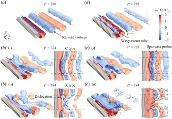
 $t^*\approx 310$
near the midspan of the cylinder and progressively spread towards the two ends over time, with occasional brief recovery of structure coherency, e.g. at
 $t^*\approx 370$
. At the same time, the amplitude of
 $C_{\kern-1pt L}$
fluctuation further diminishes from a comparably small value; see figure 16(
 $c$
i), echoing figure 8(
 $b$
). Structure coherency remains discernibly less fragmented in RII in comparison. Noting that the sampling location is at
 $x\approx L_f$
for this case, these incoherent flow structures detected here are formed upstream and subsequently advected to this point. This is aligned with figure 15(
 $b$
) that vortex shedding is of the least coherent Kármán type in the wake behind the cylinder of
 $\gamma ^*=1/6$
. Figure 17(
 $c$
i,
 $c$
ii) presents the vortex structures at two moments – before and after the onset of spanwise coherence loss (
 $t^*\approx 310$
). Vortex structures can also be categorised as C and X types, similar to the
 $\gamma ^*=1/9$
case, but with a less curved C type appearing occasionally and a more broken X type occurring frequently upstream (
 $x\leqslant 3D_i$
), though subtly reorganised downstream. This intermittency effect will be further discussed in § 4.6.
The cross-correlation of the transverse velocity
 $v$
along the spanwise direction
 $(3D_i,0,z)$
is calculated to examine the 3-D coherence in the near wake. The reference point is located at
 $(3D_i,0,L_s/2)$
. The correlation coefficient between
 $v(z)$
and
 $v(z+\Delta z)$
is calculated as
 \begin{align} R_{v_i v_j}= \frac {\langle v_i(z) \,v_j (z+\Delta z) \rangle }{\sqrt {\langle v^2_i (z)\rangle } \,\sqrt {\langle v^2_j (z+\Delta z)\rangle }}. \end{align}
Figure 18(
 $a$
) presents
 $R_{v_i v_j}$
calculated over a time period corresponding to approximately 30 vortex shedding cycles. For
 $\gamma ^* = 0$
,
 $R_{v_i v_j}$
decays slowly with increasing
 $\Delta z$
, suggesting spanwise-uniform vortex shedding. In contrast,
 $R_{v_i v_j}$
for the twisted cylinders decay more rapidly, suggesting that twisted configurations reduce the spanwise coherence of vortex shedding, making vortex shedding more 3-D, and thereby contributing to flow and noise control. Among the twisted cases,
 $\gamma ^* = 1/6$
shows the most significant reduction in spanwise correlation, consistent with its superior noise reduction performance, as shown in figure 6(
 $a$
). Additionally,
 $R_{v_i v_j}$
is recalculated for the time interval before and after
 $t^*=360$
(see figure 16
 $c$
i) to further illustrate its ability to indicate the level of spanwise coherence of the wake structure. The results are shown in figure 18(
 $b$
). It is clear that structure fragmentation (cf.
 $t^*\gt 360$
in figure 16
 $c$
ii) significantly reduces the spanwise correlation length, accompanied by the substantially weakened
 $C_{\kern-1pt L}$
fluctuation (figure 16
 $c$
i). As a result, the effective dipole source responsible for the radiated sound is markedly reduced according to Phillips (Reference Phillips1956).
Spanwise cross-correlation for all the twisted cases in (
 $a$
) and for
 $\gamma ^* = 1/6$
in (
 $b$
) over two time intervals; cf. figure 16(
 $c$
i,
 $c$
ii).

4.4. Low frequency modulation for
$\gamma ^* = 1/6$

The optimal twist
 $\gamma ^* = 1/6$
manifests interesting non-uniform characteristics in both space and time. Spatially, the regional POD analysis shown in figure 15 statistically reveals that the effective noise reduction stems from the low vortex coherency upstream,
 $x\leqslant L_f$
, echoing figure 18, despite the vortices’ reorganisation downstream. Temporally, figure 16 indicates a strong intermittent vortex shedding behaviour in RI for this case, which is supported quantitatively by Kurtosis (or flatness factor) of
 $v'$
, i.e.
 $K(v')=\overline {v'^4}/ (v'_{\textit{rms}} )^4$
, along the sampling line
 $(3D_i, 0, [0,L_s])$
. Kurtosis is often used to quantify intermittency in a turbulent flow (Davidson Reference Davidson2015). Figure 19(
 $b$
) shows that
 $K(v')$
is distinctively larger for
 $\gamma ^* = 1/6$
than other twist cases, especially over
 $0.2\lesssim z/L_s\lesssim 0.8$
, corresponding to RI.
(
 $a$
) The PSD of transverse velocity,
 $\varPhi _{\mathit{vv}}$
, within the shear layer region at the location
 $(x_\omega , y_\omega ,0.5L_s)$
, in RI. (
 $b$
) Kurtosis of
 $v'$
along the line
 $(3D_i, 0, [0,L_s])$
.

This intermittency can also be detected from the temporal behaviour within the shear layer. Figure 19(
 $a$
) presents PSD of
 $v'$
behind the midspan (
 $z/L_s=0.5$
) within RI. Unlike figure 13(
 $a$
i–
 $a$
iv), where the
 $(x,y)$
coordinates of the sampling location are fixed, here, the probe is placed as per the shedding characteristics of each case. That is, in the streamwise direction,
 $x_\omega =x_{{sep}}+0.5\overline {L}_{\omega }$
, where
 $x_{{sep}}$
stands for the
 $x$
-coordinate of the separation point. This places
 $x_\omega$
halfway into the time-averaged shear layer which is
 $\overline {L}_{\omega }$
long, see figure 10. Transversely, it corresponds to the
 $y$
-coordinate at which the time-averaged maximum
 $\omega$
magnitude occurs at
 $x_\omega$
, denoted as
 $y_\omega$
. Thus,
 $(x_\omega , y_\omega )$
varies for different cases.
As shown in figure 19(
 $a$
), in addition to the K–H instability in the shear layer reflected by the hump within
 $1\lesssim St\lesssim 4$
for all cases, consistent with figure 13(
 $a$
i–
 $a$
iv), the
 $\gamma ^*=1/6$
case shows another low frequency hump at
 $St_L$
in RI, which pertains to intermittency, namely modulation of vortex shedding, as shown in figure 21(
 $c$
). This low frequency
 $St_L\approx St_0/6$
(Kiya & Sasaki Reference Kiya and Sasaki1983) has also been observed in the wake flow behind flat plates (Wu et al. Reference Wu, Miau, Hu and Chou2005) and aerofoils (Yang et al. Reference Yang, Pröbsting, Li, Liu and Li2022), which was attributed to low-frequency oscillations of the recirculation bubble.
The configuration of
 $\gamma ^* = 1/6$
triggers a low-frequency oscillation of the recirculation bubble, which causes modulation in the flow field, leading to broader tones in RI, as shown in figures 13(
 $a$
iii) and 19(
 $a$
), unlike the single tone at
 $St_1$
in Pattern II (
 $\gamma ^* = 1/9$
). As a result, the far-field noise spectrum exhibits a blunt, broadened peak instead of clearly separated tones (figure 5
 $a$
). In addition, modulation produces a relatively stable region in RI over a specific time period (see figure 21
 $c$
) and a significant disparity in vortex shedding strength between RI and RII, which disrupts spanwise coherence (see figure 18), suppresses the dominant tone, and thus reduces noise emission.
4.5. Acoustic source strengths
The relationship between the characteristics of the near-field wake and far-field noise can be established by examining the acoustic source through the solution of the FW–H equation (3.6). For a rigid stationary surface at low Mach numbers, as discussed in § 3.1, the far-field solution can be simplified as the dipole source term (Curle Reference Curle1955; Glegg & Devenport Reference Glegg and Devenport2017),
 \begin{align} p'(\boldsymbol{x},t) \approx \frac {x_i}{4\pi |\boldsymbol{x}|^2 c_0} \int _S \left [ \frac {\partial (p_{\textit{ij}} n_{\kern-1pt j})}{\partial \tau }\right ]_{\tau =\tau ^*} \mathrm{d}S, \end{align}
where the far-field observer is located at
 $\boldsymbol{x}$
, and
 $\tau ^*=t-|\boldsymbol{x}|/c_0$
denotes the retarded time. Within the compressive stress tensor
 $p_{\textit{ij}}$
, the contribution of viscous stresses is generally much smaller than that of surface pressure fluctuations and can be neglected in far-field noise prediction (Glegg & Devenport Reference Glegg and Devenport2017). Consequently, the dipole source term in (4.2) is dominated by
 $p'$
on the cylinder surface, and the resulting far-field sound is approximately proportional to the time derivative,
 $\mathrm{d}p'/\mathrm{d}t$
. The dipole source strength on the hexagonal cylinder, denoted as
 $I_p$
, is obtained by first integrating the PSD of the pressure fluctuation derivative
 $\mathrm{d}p'/\mathrm{d}t$
over the frequency range
 $0.10 \lesssim St \lesssim 0.21$
, which well covers the dominant tones at
 $St_0$
,
 $St_1$
and
 $St_2$
in figure 5.
Contours of
 $I_p$
, normalised by
 $ U^3_\infty /D_i$
in decibels, over the cylinder surface: (
 $a$
)
 $\gamma ^* = 0$
, (
 $b$
)
 $\gamma ^* = 1/9$
, (
 $c$
)
 $\gamma ^* = 1/6$
, (
 $d$
)
 $\gamma ^* = 1/3$
. Note the different colourbar ranges. The azimuthal angle
 $\theta$
was defined in figure 1(
 $c$
). Dashed lines in (
 $b$
–
 $d$
) mark the RI/RII partition, cf. figure 9.

The contours of normalised
 $I_p$
in figure 20(
 $a$
) demonstrate that for the baseline case
 $\gamma ^* = 0$
, dipole sound sources due to vortex shedding are distributed on the leeward side, with the strongest source strength along the two PSLs
 $\theta =\pm 60^\circ$
, cf. figure 9(
 $a$
), indicating that the vicinity of PSL is the primary noise source (Oguma, Yamagata & Fujisawa Reference Oguma, Yamagata and Fujisawa2013). Applying twist significantly diminishes the
 $I_p$
level, with its maxima (see the colourbar range) consistent with
 $\Delta$
OASPL in figure 6(
 $a$
). For
 $\gamma ^*=1/9$
and
 $1/6$
in figure 20(
 $b{,}c$
), high levels of
 $I_p$
are concentrated around the base area (i.e.
 $\theta \approx \pm 180^{\circ }$
) within regime RI, different from the baseline, indicating that shear layer reattachment attenuates the noise source on the twisted cylinder. The
 $\gamma ^* = 1/6$
case shows the lowest
 $I_p$
intensity, which is associated with the weakest vortex shedding process, in line with figure 13(
 $b$
iii). For the strongest twist case
 $\gamma ^* = 1/3$
, the sound source distribution resembles the baseline case to some extent, with high intensities back to the PSL; see figure 9(
 $d$
), suggesting the classical vortex shedding (Pattern I), echoing figure 5(
 $b$
).
4.6. Discussion of control mechanisms
The experimental and numerical results shown in § 4.1–§ 4.3 have revealed that applying spanwise twist suppresses far-field noise through modifying the wake flow, though with a nonlinear dependence on the degree of twist, quantified by
 $\gamma ^*$
. Based on the four simulated cases, the following mechanisms are plausibly valid.
-
(i) A small to moderate twist in the range of
$ 1/18 \leqslant \gamma ^* \leqslant 1/7.2$
results in the emergence of dual tones in the noise spectrum with similar intensities substantially lower than that of the straight cylinder, leading to a noise reduction effect. This corresponds to Pattern II of vortex shedding where the mismatch of the two frequencies in RI and RII (figure 13) leads to vortex dislocation, namely the temporally alternating C- and X-type flow structures, as illustrated in figure 21(
$b$
). -
(ii) Further increasing the twist to
$1/5.4\leqslant \gamma ^*\leqslant 1/3$
reduces the number of tones in the noise spectrum back to one (the same for the straight cylinder), corresponding to the classical Kármán vortex shedding, Pattern I. However, the spanwise twist induces wavy vortex tubes, lowering the shedding coherency compared with the straight cylinder, thereby achieving a noise reduction effect that is weaker than Pattern II. This is illustrated in figure 21(
$a$
). -
(iii) At
$\gamma ^* = 1/6$
, or a nearby twist value, the mechanism appears to be a superposition of the two described above, corresponding to a transitional state between Patterns I and II, as illustrated in figure 21(
$c$
). This is supported by the moderate curvature of the C-type structure and the more broken X-type structure, compared with those in Pattern II, see figure 17. Additionally, modulation of vortex shedding in RI further weakens vortex shedding. These result in a blunt peak in the noise spectrum, intermediate between the single tone and dual tones of the two patterns (figure 5), consequently yielding a remarkable and optimal noise reduction effect, especially at high
$ \textit{Re}$
(see figure 6).


Schematic diagram illustrating the flow and noise control mechanisms of the twisted cylinders for (
 $a$
) Pattern I, (
 $b$
) Pattern II and (
 $c$
) transitional pattern (
 $\gamma ^* = 1/6$
).

5. Conclusions
In the present study, far-field noise experiments were conducted to investigate aerodynamic noise radiated from hexagonal cylinders with different twist angles (
 $0\lt \gamma ^* \leqslant 1/3$
) at
 $ \textit{Re} = 2\times 10^4$
–
 $10^5$
. The twist angle was found to play a significant role in noise reduction, although its effect does not vary monotonically with the angle. As
 $\gamma ^*$
decreases, the OASPL initially decreases and then increases. The maximum noise reduction occurs for
 $\gamma ^* = 1/6$
, where the reduction in the tonal peak reached 15 dB, and the OASPL was reduced by 11 dB. Furthermore, the noise reduction was found to be independent of Reynolds number variations within the subcritical regime. In addition, dual-tone phenomena were observed in the noise spectra for
 $1/18\leqslant \gamma ^*\lt 1/6$
. Based on the number of tones, the twisted cylinders were categorised into two flow patterns: Pattern I (single tone), corresponding to the classical von Kármán vortex shedding mode; and Pattern II (dual tones), corresponding to a spanwise dislocated vortex shedding mode, as well as a transitional state between Patterns I and II.
To further explore the flow and noise control mechanisms, numerical simulations were performed for selected cases (
 $\gamma ^* = 1/9$
,
 $1/6$
and
 $1/3$
) at
 $ \textit{Re} = 2\times 10^4$
. The flow separation, shear layer behaviour and wake characteristics were analysed to understand the 3-D vortex shedding processes, and an analysis of wall shear stress was performed to identify the flow separation and reattachment regimes. Twisted cylinders exhibited different ranges of separation (RI) and reattachment (RII) regimes along the span. This variation in flow separation results in different shear layer lengths, with the shear layer in RI being shorter than that in RII, related to more stable shear layer in the RII regime.
The emergence of 3-D coherent structures caused by the spanwise variation of flow separation was observed in the near wake of the twisted cylinders. Significant reductions in
 $v'_{\textit{rms}}$
were found, which is closely related to tonal noise levels, especially for
 $\gamma ^* = 1/6$
. The wavy vortex shedding observed in
 $\gamma ^* = 1/3$
was confirmed through POD modes in the
 $x$
–
 $z$
plane, providing insights into the noise reduction mechanism for Pattern I. For
 $\gamma ^* = 1/9$
(Pattern II), dual peaks were found in the spectra of both wake flow velocity and far-field noise. The POD analysis further confirmed the presence of two distinct flow patterns. Pattern II, pertaining to vortex dislocation, is induced by different vortex shedding frequencies in RI and RII, leading to the formation of C-type and X-type vortex structures, which is associated with a greater noise reduction. For
 $\gamma ^* = 1/6$
(transitional pattern), the observed low-frequency modulation in the RI regime leads to significant intermittency and a marked difference in vortex shedding intensity between RI and RII, disrupting spanwise coherence. Together with the frequent vortex dislocation revealed by POD analysis, these mechanisms jointly contribute to the superior noise reduction performance of the
 $\gamma ^* = 1/6$
configuration.
Acknowledgements
The authors are grateful for the support from the Centre for Computational Science and Engineering at Southern University of Science and Technology.
Funding
This research was supported by the National Natural Science Foundation of China (grant no. 12111530102), the Royal Society International Exchanges (grant no. IEC/NSFC/201061) and the Department of Science and Technology of Guangdong Province (grant no. 2023B1212060001).
Declaration of interests
The authors report no conflict of interest.
Appendix A. Mesh convergence study
Time-averaged quantities used for the grid sensitivity analysis were obtained over 30 vortex shedding cycles after a quasisteady state was reached. As shown in table 2, the time-averaged drag coefficient
 $\overline {C}_{\kern-1pt D}$
and the Strouhal number
 $St_0$
of vortex shedding demonstrate a good agreement with the previous LES results by Masoudi et al. (Reference Masoudi, Gan and Sims-Williams2021) and are slightly greater than the experimental results in Xu et al. (Reference Xu, Zhang, Gan, Li and Zhou2017). The medium grid was selected after striking a balance between the LES resolution and computational efficiency.
Comparison of aerodynamic parameters for the hexagonal cylinder in corner orientation, between the present and previous numerical studies performed at
 $ \textit{Re} = 10^4$
and experimental studies at
 $ \textit{Re} = 2\times 10^4$
. Here
 $N_r$
,
 $N_\theta$
and
 $N_z$
represent the number of grid points in the radial, azimuthal and spanwise directions, respectively.

The influence of spanwise grid resolution was examined on the strongest twist case (
 $\gamma ^* = 1/3$
). The resolution in the cross-sectional plane holds constant with
 $N_r \times N_\theta = 264\times 264$
, whereas the grid point number in the spanwise
 $z$
-direction varies from 60 to 92. Table 3 reflects a negligible impact on
 $\overline {C}_{\kern-1pt D}$
and
 $St_0$
. To balance computational cost and accuracy, the spanwise resolution of
 $N_z = 76$
was adopted in the simulations. As
 $L_s$
increases with decreasing
 $\gamma ^*$
,
 $N_z$
was set to 152 and 228 for
 $\gamma ^* = 1/6$
and
 $1/9$
, respectively, in order to maintain a consistent grid resolution along the span.
Comparison of aerodynamic parameters for the case
 $\gamma ^* = 1/3$
between different spanwise mesh resolutions at
 $ \textit{Re} = 2\times 10^4$
.

Appendix B. Further experimental validation
A time-resolved stereoscopic PIV (TR-SPIV) measurement was performed to capture the velocity field in the cylinder near wake. The in-plane flow distribution over the
 $x$
–
 $z$
plane at
 $y=0$
is used to validate the current numerical framework. Figure 22 presents a schematic of the experimental set-up. The flow in the wind tunnel was uniformly seeded with approximately 1
 $\unicode{x03BC}$
m oil droplets of Di(2-ethylhexyl) sebacate generated by an aerosol generator, and was illuminated using a double-pulsed Nd:YAG laser (527 nm, 50 mJ per pulse at 1 kHz, Photonics). The laser beam was shaped into a light sheet of approximately 5 mm thick. The laser beam was directed upstream in a forward-scattering configuration.
Schematic of the TR-SPIV experimental set-up: (a) side view; (b) top view.

Comparison of time-averaged streamwise velocity (
 $\overline {u}/U_{\infty }$
) distribution between numerical simulations and experiments at
 $ \textit{Re} = 2 \times 10^4$
: (
 $a$
)
 $\gamma ^* =0$
, (
 $b$
)
 $\gamma ^* =1/9$
, (
 $c$
)
 $\gamma ^* =1/6$
and (
 $d$
)
 $\gamma ^* =1/3$
.

Two 12-bit high-resolution CCD cameras (
 $1280\times 800$
pixels, pixel pitch 20
 $\unicode{x03BC}$
m, Phantom VEO 410L) equipped with Micro-Nikkor 60 mm f/2.8 lenses were used for image acquisition. The cameras were positioned at an angle of approximately
 $45^\circ$
to the field of view (FOV). Sheimpflug adaptors were used to ensure image focus. The laser and cameras were synchronised via a LaVision Programmable Time Unit to achieve a sampling rate of 1000 frame pairs per second and 2 s of sample duration. The acquired instantaneous images were processed using an iterative multigrid multipass process with window deformation. The final interrogation window size was
 $32\times 32$
pixels with 75 % overlap, resulting in a spatial resolution of 7.41 mm based on interrogation window size. The centre of the FOV was set at cylinder midspan
 $z_0$
with the left-hand edge at
 $x\approx 1.1D_i$
. After cropping, the final FOV size is approximately
 $9.8D_i\times 10.8D_i$
in the streamwise and spanwise directions, respectively.
Comparison of the time-averaged streamwise velocity
 $\overline {u}$
between numerical simulations and experiments at
 $ \textit{Re} = 2 \times 10^4$
(figure 23) shows reasonable agreement for all
 $\gamma ^*$
, reassuring the reliability of the adopted numerical scheme. The only noticeable discrepancy occurs in the case
 $\gamma ^* = 1/6$
, where the recirculation region from the experiment is slightly larger than the simulation result. Nevertheless, the overall distribution of
 $\overline {u}$
remains consistent between the two.
Appendix C. Spanwise correction for acoustic prediction
As the twist wavelength
 $L_s$
, which is also the span used for simulations, varies with
 $\gamma ^*$
and is much smaller than the span length of cylinder models tested experimentally, a direct comparison between the numerical and experimental results of far-field noise can be misleading, making a spanwise correction to the predicted
 $\varPhi _{pp}$
necessary. Following Kato et al. (Reference Kato, Iida, Takano, Fujita and Ikegawa1993), the correction for the far-field acoustic PSD calculated from simulations,
 $\varPhi _{pps}$
, can be written as
 \begin{align} \varPhi _{pp}= \begin{cases} \varPhi _{pps}+10\log _{10}\left ({L}/{L_s}\right ), & L_c \leqslant L_s; \\ \varPhi _{pps}+20\log _{10}\left ({L_c}/{L_s}\right ) + 10\log _{10}\left ({L}/{L_c}\right ), & L_s \leqslant L_c \leqslant L_e; \\ \varPhi _{pps}+20\log _{10}\left ({L}/{L_s}\right ), & L \leqslant L_c. \end{cases} \end{align}
In (C1),
 $L_e$
is the span of the cylinder model used in experiments,
 $L_c$
denotes the spanwise coherence length of the cylinder, and the target span
 $L$
for correction, which can be arbitrary, equals
 $L_e$
in the present study. It is worth noting that the correction method of Kato et al. (Reference Kato, Iida, Takano, Fujita and Ikegawa1993) was originally developed for sound pressure level (SPL). Since both PSD and SPL scale with
 $\log _{10}(p'^2)$
, this method is also applicable to
 $\varPhi _{pp}$
.
In the present study, the spanwise coherence length
 $L_c$
, which is a function of
 $f$
, is defined as the distance from a reference point to the location where the coherence level drops to a critical value. For
 $\gamma ^* = 0$
(spanwise homogeneous case), the coherence length was determined to be
 $L_c = 3.4L_s$
at
 $St_0$
using a Gaussian fit and the critical coherence value of 0.7. Note that the critical value of 0.5 was used by Kato et al. (Reference Kato, Iida, Takano, Fujita and Ikegawa1993) for circular cylinders, which was rather ad hoc to achieve a reasonable agreement with experiments. Therefore, in this study, a larger critical coherence of 0.7 was taken, because the straight hexagonal cylinder has higher spanwise coherence (see figure 17
 $a$
), due to stronger flow separation, than a circular cylinder. In contrast, for twisted cylinders, periodic reattachment within each wavelength
 $L_s$
disrupts the spanwise coherence, resulting in nearly independent local flow structures along the span (see figure 13). For this reason, the acoustic sources can be regarded as incoherent within each wavelength segment, which contribute to the far-field noise independently. Consequently, for numerical predictions of far-field acoustic PSD, the correction term to compensate for the larger cylinder span used in experiments than simulations becomes simply
 $L_e/L_s$
, i.e. the first expression in (C1).