1. INTRODUCTION
Vision-aided inertial navigation systems have been extensively studied (Kelly and Sukhatme, Reference Kelly and Sukhatme2011; Feng et al., Reference Feng, Wu and Wang2012; Weiss et al., Reference Weiss, Achtelik, Lynen, Chli and Siegwart2012; Kottas and Roumeliotis, Reference Kottas and Roumeliotis2013; Hesch et al., Reference Hesch, Kottas, Bowman and Roumeliotis2014; Xian et al., Reference Xian, Hu and Lian2015; Liu et al., Reference Liu, Sarvrood and Gao2018), as IMUs and vision systems have complementary features. For example, IMUs have the ability to capture fast ego-motion with lower uncertainty, while cameras can track feature points precisely in slow motion. This kind of integrated system can operate in environments where Global Navigation Satellite Systems (GNSS) are unreliable or unavailable. Corke et al. (Reference Corke, Lobo and Dias2007), made a comprehensive introduction of loosely-coupled and tightly-coupled vision and IMU integration systems. Loosely-coupled vision and IMU integration systems fuse the inertial navigation solution with relative pose estimation between consecutive image measurements (Tardif et al., Reference Tardif, George, Laverne, Kelly and Stentz2010; Sirtkaya et al., Reference Sirtkaya, Seymen and Alatan2013). Tightly-coupled methods, in contrast, process the raw information of both sensors in a single estimator, thus leading to higher accuracy (Mourikis and Roumeliotis, Reference Mourikis and Roumeliotis2007). A kind of vision-aided inertial tightly-coupled mechanisation which is based on tri-focal tensor geometry has been studied by many researchers (Asadi and Bottasso, Reference Asadi and Bottasso2012; Indelman et al., Reference Indelman, Gurfil, Rivlin and Rotstein2012; Fang and Huang, Reference Fang and Huang2013). For feature extraction, it is better to use both the lines and the points, because they can provide complementary information about the image (Zhang, Reference Zhang2013; Kitt et al., Reference Kitt, Geiger and Lategahn2010). Hu and Chen (Reference Hu and Chen2014) proposed a sliding window odometry using monocular camera geometry constraints among three images as measurements; the results showed that the mechanisation worked well, when point and line features were used. Experiments by Kong et al. (Reference Kong, Wu, Zhang and Wang2015), also showed that by using both point and line features, navigation accuracy was better than by merely using point features. An Unscented Kalman Filter (UKF) was used in the works by Hu and Chen (Reference Hu and Chen2014) and Kong et al. (Reference Kong, Wu, Zhang and Wang2015).
However, UKF may have some problems, since it cannot guarantee the stability of the tightly-coupled system, and it has to re-determine the positive definiteness of the estimation covariance matrix. Square-Root Unscented Kalman Filter SRUKF (Merwe et al., Reference Merwe and Wan2001) is an improvement of UKF, which uses QR decomposition (where Q is an orthogonal matrix and R is an upper triangular matrix) instead of Cholesky decomposition as in UKF. This can not only avoid the most expensive operation by merely calculating the square-root of the state covariance at each time updating, but also guarantees the positive semi-definiteness of the state covariance to ensure the stability of the computation. From this perspective, SRUKF is a better filter method to replace UKF. Based on this fact, Xian et al. (Reference Xian, Lian, Shan, Zhang, He and Hu2016), presented a SRUKF-based binocular stereo Vision/IMU tightly-coupled system, among which multiple view geometry constraints were used. The results indicated that this mechanisation provided benefits over that identified in Hu and Chen (Reference Hu and Chen2014).
However, the standard SRUKF uses 2n + 1 sigma points for the UT which will affect the computation time. UT methods have some variants with reduced sigma sets. For example, the simplex sigma set uses n + 2 sigma points (Julier et al., Reference Julier and Uhlmann2002). However, this kind of UT method has the problem that the radius which bounds the sphere of the sigma points is 2n/2. Therefore, at even relatively low dimensions, there are potential problems with numerical stability. The spherical simplex sigma set uses n + 2 sigma points (Julier et al., Reference Julier2003). The sigma points lie in the hypersphere with a radius of 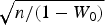 $\sqrt{n/\lpar 1-W_{0}\rpar }$, and this had better stability than the earlier proposal. Menegaz et al. (Reference Menegaz, Ishihara and Borges2011), proposed a minimum sigma set UT by using only n + 1 sigma points, and the experiments in this paper showed that this algorithm worked well. A novel simplex unscented transform and filter was proposed by Li et al. (Reference Li, Wei and Xiao2007), which also used n + 1 sigma points. The UKF and SRUKF family were systematically illustrated by Menegaz et al. (Reference Menegaz, Ishihara, Borges and Vargas2015). There are some conceptual statements in the reduced sigma point set section, and they are revised through theoretical analysis (Wang et al., Reference Wang, Wu and El-sheimy2017).
This paper introduces the quadrifocal tensor constraints in a binocular Vision-IMU tightly-coupled system. As far as the authors are aware, this is the first time that a quadrifocal tensor has been used in a real time positioning and navigation system. The structure of the binocular vision-IMU tightly-coupled system is in the form of error state, and the time updates of the state and the state covariance are directly estimated without using UT transformation. In order to further save computation cost, M-SRUKF is used in the binocular vision-IMU tightly-coupled system.
Several ego-motion cases from both outdoor and indoor open source datasets are used for evaluating the performance of the new algorithms. Results showed that the new M-SRUKF based binocular vision-IMU mechanisation by using four views geometry performs well in all the test cases.
2. VISION-IMU TIGHTLY-COUPLED SYSTEM MODEL
The reference frames and system model used in the vision-IMU tightly-coupled system are defined as follows (Xian et al., Reference Xian, Lian, Shan, Zhang, He and Hu2016).
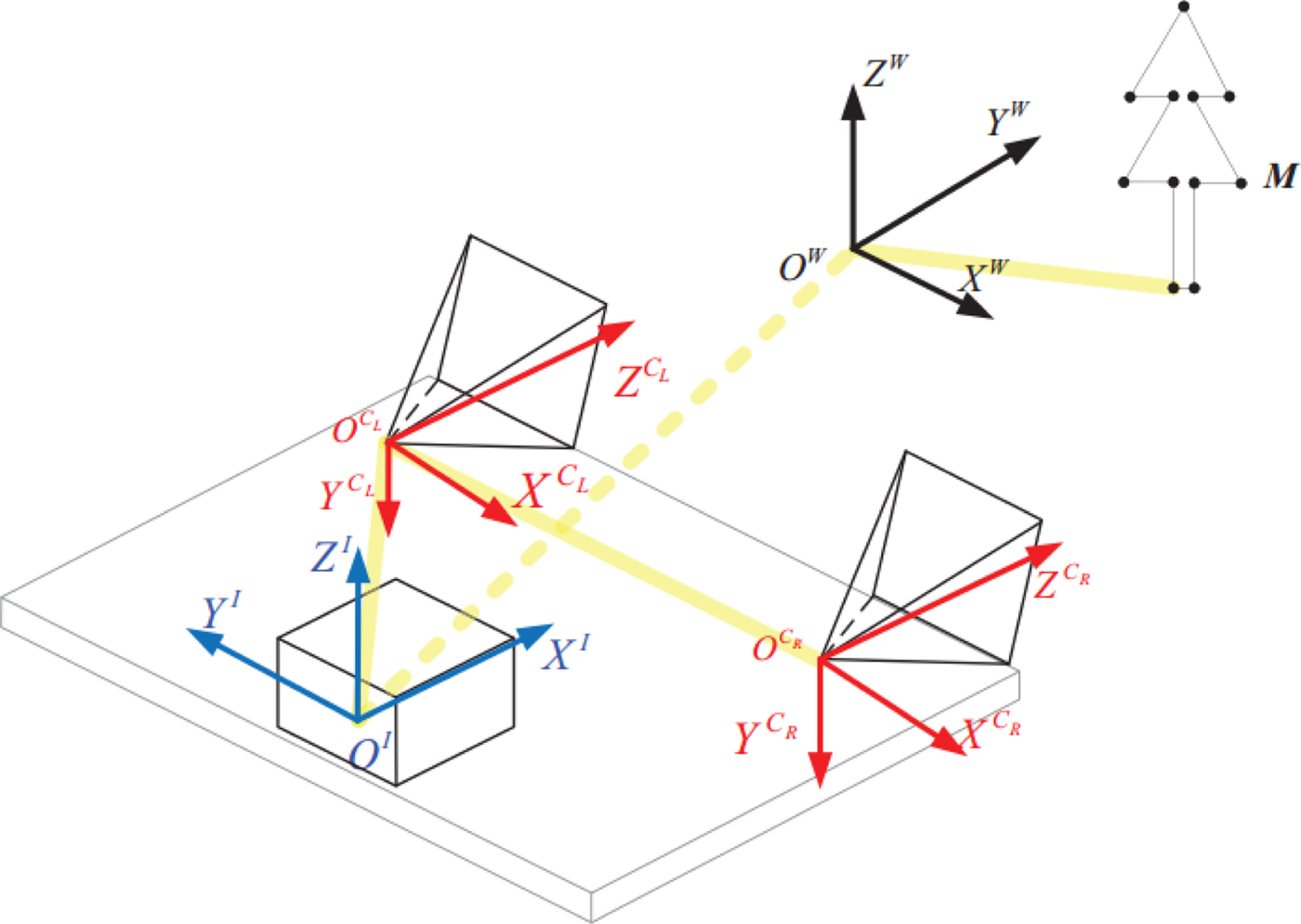
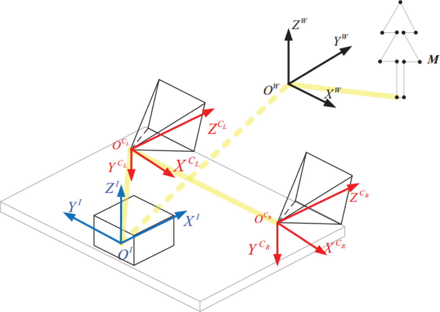
Figure 1 shows the relationships of the three reference frames. The W frame is the world frame, where the pose of the IMU is estimated with respect to this frame. The C frame is the camera frame, where C L is the left camera, C R is the right camera, and they are rigidly attached. The I frame is the IMU frame, with origin at the centre of the IMU body. The feature points M are modelled in the world frame W.
Reference frames and their relationships.
The IMU state vector is defined as:
 $${\bf x}_{IMU} \lpar t\rpar =\left[\matrix{{\lpar {\bar{\bi q}}_{WI}\rpar^T} & {\lpar {\bi v}_{WI}^W \rpar^T} & {\lpar {{\bi p}_{WI}^W }\rpar^T} & {\lpar {{\bi b}_g \lpar t\rpar }\rpar^T} & \lpar {{\bi b}_a \lpar t\rpar }\rpar^T & {}^1\lpar {\bar{\bi q}}_{WI}\rpar^T & {}^1\lpar {{\bi p}_{WI}^W }\rpar^T}\right]^T$$
where  ${\bi p}_{WI}^{W} \lpar t\rpar $ represents the position of IMU in the world frame {W};
 ${\bar{\bi q}}_{WI} \lpar t\rpar $ is the unit quaternion of the IMU frame {I} in the world frame;
 ${\bi v}_{WI}^{W}$ is the linear velocity of the IMU in the world frame; bg(t) and ba(t) are the IMU gyroscope and accelerometer biases, respectively.
 $\lpar {}^{1}\lpar \bar{\bi q}_{WI}\rpar^{T}\comma \; {}^{1}\lpar {\bi p}_{WI}^{W}\rpar^{T}\rpar $ denotes the last pose of the IMU respect to the frame {W}.
The biases bg(t) and ba(t) are modelled as a Gaussian random walk process, driven by the white, zero-mean noise vectors ngw and naw, with covariance matrices Qgw and Qaw, respectively. The time evolution of the IMU state is given by the following equation (Kelly et al., Reference Kelly and Sukhatme2011):
 $${\dot{\bi p}}_{WI}^W ={\bi v}_{WI}^W \comma \; {\dot{\bar{\bi q}}}_{WI} =\displaystyle{{1}\over{2}}\Omega \lpar {{\bf \omega}_{WI}^I}\rpar {\bar{\bi q}}_{WI} \comma \; \quad {\dot{\bi v}}_{WI}^W ={\bi a}_{WI}^W \comma \; {\dot{\bi b}}_g =n_{gw} \comma \; {\dot{\bi b}}_a ={\bi n}_{aw} $$
where the  $\Omega \lpar {{\bf \omega}_{WI}^{I} }\rpar $ is the quaternion multiplication matrix shown in Equation (3):
 $$\Omega \lpar {{\bf \omega}_{WI}^I }\rpar =\left[\matrix{ 0 & {-\lpar {{\bf \omega}_{WI}^I }\rpar^T} \cr {{\bf \omega}_{WI}^I } & {-\lsqb {{\bf \omega}_{WI}^I \times}\rsqb }}\right]$$
where  ${\bf \omega}_{WI}^{I}$ is the angular velocity of the IMU with respect to the world frame, and
 ${\bi a}_{WI}^{W}$ is the acceleration of the IMU with respect to the world frame expressed in the world frame. The measured angular velocity and linear acceleration are:
 $${\bf \omega}_m ={\bf \omega}_{WI}^I +{\bi b}_g +{\bi n}_g $$
 $${\bi a}_m ={\bi R}^T\lpar {{\bar{\bi q}}_{WI}}\rpar \lpar {{\bi a}_{WI}^W -{\bi g}^W}\rpar +{\bi b}_a+{\bi n}_a $$
where  ${\bi R}\lpar {{\bar{\bi q}}_{WI}}\rpar $ is the direction cosine matrix corresponding to the unit quaternion
 ${\bar{\bi q}}_{WI} $, ng and na are measurements of the noise of the gyroscope and accelerometer, which are assumed to be zero-mean Gaussian noise with covariance matrices Qg and Qa, respectively. In the models, the Earth's rotation rate was not considered in the gyroscope measurement, because it is small enough relative to the noise and bias of the low-cost gyroscope.
The filter error state vector for the Kalman filter is defined as:
 $$\delta {\bf x}=\left[\matrix{{\lpar {\delta {\bf \theta}^I}\rpar^T} & {\lpar {\delta {\bi v}_{WI}^W }\rpar^T} & {\lpar {\delta {\bi p}_{WI}^W }\rpar^T} & \delta {\bi b}_g^T & \delta{\bi b}_a^T & {}^1\lpar \delta {\bf \theta}^I\rpar^T & {}^1\lpar \delta {\bi p}_{WI}^W\rpar^T}\right]^T $$
The differential equation for the previous pose  $\lpar {{}^{1}\lpar {{\bar{\bi q}}_{WI}}\rpar^{T}\comma \; {}^{1}\lpar {{\bi p}_{WI}^{W}}\rpar^{T}}\rpar $ is defined as indicated in Equation (7):
 $${}^1{\dot{\bi q}}_{WI} =0\comma \; {}^1{\dot{\bi p}}_{WI}^W =0 $$
The error-state process model is defined as:
 $$\delta {\dot{\bf x}}=F\delta {\bf x}+{\bi n} $$
where:
 $$\eqalign{F & =\left(\matrix{{F_{11}} & {{\bf 0}_{15\times 6}} \cr {F_{21}} & {{\bf 0}_{6\times 6}} \cr}\right)\cr {\bi n} & =\left(\matrix{{{\bf 0}_{9\times 1}^T } & {{\bi n}_g^T } & {{\bi n}_a^T } & {{\bf 0}_{6\times 1}^T }}\right)^T \cr F_{11} & =\left(\matrix{ {\lsqb \lpar {{\bi b}_g -{\bf \omega}_m }\rpar \times \rsqb } & {{\bf 0}_{3\times 3}} & {{\bf 0}_{3\times 3}} & {-{\bi I}_3 } & {{\bf 0}_{3\times 3}} \cr {{\bi R}\lpar {{\bar{\bi q}}_{WI}}\rpar \lsqb \lpar {{\bi b}_a -{\bi a}_m }\rpar \times \rsqb } & {{\bf 0}_{3\times 3}} & {{\bf 0}_{3\times 3}} & {{\bf 0}_{3\times 3}} & {-{\bi R}\lpar {{\bar{\bi q}}_{WI}}\rpar } \cr {{\bf 0}_{3\times 3}} & {{\bi I}_3} & {{\bf 0}_{3\times 3}} & {{\bf 0}_{3\times 3}} & {{\bf 0}_{3\times 3}} \cr {{\bf 0}_{6\times 3}} & {{\bf 0}_{6\times 3}} & {{\bf 0}_{6\times 3}} & {{\bf 0}_{6\times 3}} & {{\bf 0}_{6\times 3}} \cr}\right)\cr F_{21} & =\left(\matrix{ {{\bi I}_3 } & {{\bf 0}_{3\times 3}} & {{\bf 0}_{3\times 3}} & {{\bf 0}_{3\times 3}} & {{\bf 0}_{3\times 3}} \cr {{\bf 0}_{3\times 3}} & {{\bf 0}_{3\times 3}} & {{\bi I}_3 } & {{\bf 0}_{3\times 3}} & {{\bf 0}_{3\times 3}} \cr}\right)} $$
3. QUADRIFOCAL TENSOR BASED CONSTRAINTS
The measurement constraints used in this paper are the epipolar constraint between two images, the trifocal tensor constraint among three images and the quadrifocal tensor constraint among four images. The epipolar constraint and the trifocal tensor constraint are the same as described in Hu et al. (Reference Hu and Chen2014), Kong et al. (Reference Kong, Wu, Zhang and Wang2015) and Xian et al. (Reference Xian, Lian, Shan, Zhang, He and Hu2016). The left and right images at the earlier time are denoted respectively by Im1 and Im2, and those in the current view are denoted by Im3 and Im4. The epipolar constraints used for measurement are the pairs (Im1, Im3) and (Im2, Im4). These two pairs are chosen because they contain the relative pose information between the previous and current poses, which is helpful in improving the accuracy of the state estimates. Similarly, the trifocal tensor constraints used in the measurement are groups (Im1, Im2, Im3) and (Im1, Im2, Im4). The quadrifocal tensor constraint is among the four views (Im1, Im2, Im3, Im4).
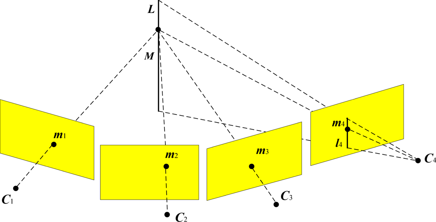
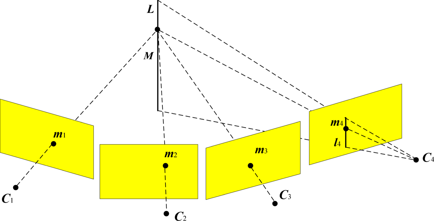
The quadrifocal tensor geometry is shown in Figure 2. The camera matrices are defined as P1 = [I|0], P2 = [A|a4], P3 = [B|b4] and P4 = [C|c4], which correspond to the different viewpoints C1, C2, C3 and C4. The normalised feature points  ${\tilde{\bi m}}_{1}\leftrightarrow {\tilde{\bi m}}_{2}\leftrightarrow {\tilde{\bi m}}_{3}\leftrightarrow {\tilde{\bi m}}_{4}$ across four views are considered (the feature points are normalised corresponding to m1 ↔ m2 ↔ m3 ↔ m4).
Point-point-point-line correspondence among four views.
A common method for deriving the quadrifocal tensor is to define the linear system as (Hartley et al., Reference Hartley and Zisserman2003):
 $$\left[\matrix{ {{\bi P}_1} & {{\tilde{\bi m}}_1} & & & \cr {{\bi P}_2} & & {{\tilde{\bi m}}_2} & & \cr {{\bi P}_3} & & & {{\tilde{\bi m}}_3} & \cr {{\bi P}_4} & & & & {{\tilde{\bi m}}_4} \cr}\right]\left(\matrix{ {\bi X} \cr {-k_1 } \cr {-k_2 } \cr {-k_3 } \cr {-k_4 } \cr }\right)=0 $$
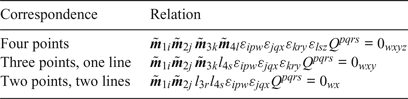
where X represents a point in Euclidean space. Since this equation has a solution, the matrix on the left in Equation (10) has rank at most 7, and so all 8 × 8 determinants are zero. Such a determinant leads to a quadrilinear relationship of the form:
Quadrilinear relations.

where each choice of the free variables w, x, y and z gives a different equation, and the four-dimensional quadrifocal tensor Q pqrs is defined by:
 $$Q^{pqrs}=\det \left[\matrix{{\bi p}_1^p \cr {\bi p}_2^q \cr {\bi p}_3^r \cr {\bi p}_4^s}\right]$$
In this paper, point-point-point-line correspondence is used for creating the four view measurement equations. The reason for this choice is that by merely using point features, the badly distributed feature points in some frames will lead to a bad orientation estimation (Kong et al., Reference Kong, Wu, Zhang and Wang2015). The measurement model is created by choosing four combinations of w, x, y and z:
 $$z_1 =\left[\matrix{ {0_{111}} \cr {0_{222}}\cr{0_{333}}\cr{0_{123}}\cr}\right]=h\lpar {\bi x}_k \comma \; {\bi m}_1 \comma \; {\bi m}_2 \comma \; {\bi m}_3 \comma \; {\bi m}_4 \rpar =\left[\matrix{ \tilde{{\bi m}}_{1i}\tilde{{\bi m}}_{2j}\tilde{{\bi m}}_{3k}l_{4s}\varepsilon_{ip1} \varepsilon_{jq1} \varepsilon_{kr1} Q^{pqrs} \cr \tilde{{\bi m}}_{1i}\tilde{{\bi m}}_{2j}\tilde{{\bi m}}_{3k}l_{4s}\varepsilon_{ip2} \varepsilon_{jq2} \varepsilon_{kr2} Q^{pqrs} \cr \tilde{{\bi m}}_{1i}\tilde{{\bi m}}_{2j}\tilde{{\bi m}}_{3k}l_{4s}\varepsilon_{ip3} \varepsilon_{jq3} \varepsilon_{kr3} Q^{pqrs} \cr \tilde{{\bi m}}_{1i}\tilde{{\bi m}}_{2j}\tilde{{\bi m}}_{3k}l_{4s}\varepsilon_{ip1} \varepsilon_{jq2} \varepsilon_{kr3} Q^{pqrs}}\right]$$
The epipolar and the trifocal tensor constraints are defined in Equation (13) (Xian et al., Reference Xian, Lian, Shan, Zhang, He and Hu2016):
 $${\bi z}_2 =\left[\matrix{ 0\cr0\cr{{\bi m}_3 }\cr{{\bi m}_4 }\cr}\right]=h\lpar {\bi x}_k \comma \; {\bi m}_1 \comma \; {\bi m}_2 \comma \; {\bi m}_3 \comma \; {\bi m}_4 \rpar =\left[\matrix{ \tilde{{\bi m}}_3^T {\bi R}_{1\comma 3}^T \lsqb {{\bi t}_{1\comma 3} \times }\rsqb \tilde{{\bi m}}_1 \cr \tilde{{\bi m}}_4^T {\bi R}_{2\comma 4}^T \lsqb {{\bi t}_{2\comma 4} \times }\rsqb \tilde{{\bi m}}_2 \cr {\bi K}_1 \left({\sum\limits_i{\tilde{{\bi m}}_{1i}{}^1{\bi T}_i^T }}\right)l_2 \cr {\bi K}_2 \left({\sum\limits_i{\tilde{{\bi m}}_{1i}{}^2{\bi T}_i^T }}\right)l_2 }\right]$$
The measurement models using the epipolar constraint, the trifocal tensor constraint and the quadrifocal tensor constraint can be described as:
 $$z=\left[\matrix{ {{\bi z}_1 }\cr{{\bi z}_2 }\cr}\right]$$
In Equations (13) and (14), {m1, m2, m3, m4} are the feature points corresponding to the four images;  $\tilde{{\bi m}}_{1i}$ is the i-th element of vector
 $\tilde{{\bi m}}_{1}$,
 $\tilde{{\bi m}}_{2j}$ is the j-th element of vector
 $\tilde{{\bi m}}_{2}$,
 $\tilde{{\bi m}}_{3k}$ is the k-th element of vector
 $\tilde{{\bi m}}_{3}$,
 $\tilde{{\bi m}}_{4l}$ is the l-th element of vector
 $\tilde{{\bi m}}_{4}$;
 $\tilde{{\bi m}}_{1}$ equals
 ${\bi K}_{1}^{-1}{\bi m}_{1}$,
 $\tilde{{\bi m}}_{2}$ equals
 ${\bi K}_{2}^{-1}{\bi m}_{2}$,
 $\tilde{{\bi m}}_{3}$ equals
 ${\bi K}_{1}^{-1}{\bi m}_{3}$ and
 $\tilde{{\bi m}}_{4}$ equals
 ${\bi K}_{2}^{-1}{\bi m}_{4}$.
 ${\bi p}_{1}^{p} \comma \; {\bi p}_{2}^{q} \comma \; {\bi p}_{3}^{r} \comma \; {\bi p}_{4}^{s}$ denote the p-th, q-th, r-th and s-th row of the projection matrices P1, P2, P3, P4, respectively. K1 and K2 are the camera intrinsic parameter matrices of the left and right cameras, respectively. 1T and 2T are the trifocal tensors of the views (Im1, Im2, Im3) and (Im1, Im2, Im4), respectively. [tj,j+2 × ] and Rj,j+2 are the position and rotation matrix of the frame C j+2 with respect to the frame C j, respectively. The lines l2, l 4 are recommended choices as the lines perpendicular to the epipolar lines (Hartley et al., Reference Hartley and Zisserman2003).
The tensor εijk is defined as (Hartley et al., Reference Hartley1998):
 $$\varepsilon _{ijk} = \left\{\matrix{ 0\comma \; & \hbox{unless}\, i\comma j\comma k\, \hbox{are distinct}\hfill \cr +1\comma \; & \hbox{if}\, i\comma j\comma k\, \hbox{are an even permutation of}\, 1\comma 2\comma 3\cr-1\comma \; & \hbox{if}\, i\comma j\comma k\, \hbox{are an odd permutation of}\, 1\comma 2\comma 3\cr}\right. $$
The rotational and translational relationship between the IMU and different views of the Camera (which is used in Equations (12) and (13)) are derived below.
We denote that TIW and 1TIW are the transformation matrices from frame {W} to frame {I} at the current time and last time, respectively; TCI are the transformation matrices from frame {I} to frame {C L}; TC1W are the transformation matrices from frame {W} to first view camera frame {C 1}; TC3W are the transformation matrices from frame {W} to third view camera frame {C 3}; RC1W and RC3W are the rotation matrices from frame {W} to {C 1} and {C 3}, respectively; tWC1 is the translational vector from {C 1} to {W} with respect to {C 1} and tWC3 is the translational vector from {C 3} to {W} with respect to {C 3}.
Then TIW and 1TIW can be expressed as:
 $$\eqalign{{\bi T}_{IW} & = \left[\matrix{\lpar {{\bi R}\lpar {\bar{\bi q}}_{WI}\rpar }\rpar^T \quad -\lpar {{\bi R}\lpar {\bar{\bi q}}_{WI}\rpar }\rpar^T{\bi p}_{WI}^W \cr {\matrix{ {0} & 0 & 0 & 1}}}\right]\cr {}^1{\bi T}_{IW} & =\left[\matrix{\lpar {{\bi R}\lpar {{}^1\lpar {{\bar{\bi q}}_{WI}}\rpar }\rpar }\rpar^T\quad -\lpar {{\bi R}\lpar {{}^1\lpar {{\bar{\bi q}}_{WI}}\rpar }\rpar }\rpar^T{}^1\lpar {{\bi p}_{WI}^W }\rpar \cr \matrix{ {0} & 0 & 0 & 1}}\right]} $$
with:
 $$\matrix{{\eqalign{&{{\bi T}_{C1W} ={\bi T}_{CI}^1{\bi T}_{IW}} \cr & {{\bi R}_{C1W} ={\bi T}_{C1W} \lpar {1\colon 3\comma \; 1\colon 3}\rpar } \cr & {{\bi t}_{WC1} ={\bi T}_{C1W} \lpar {1\colon 3\comma \; 4}\rpar }}} & {\eqalign{&{{\bi T}_{C3W} ={\bi T}_{CI} {\bi T}_{IW}} \cr & {{\bi R}_{C3W} ={\bi T}_{C3W} \lpar {1\colon 3\comma \; 1\colon 3}\rpar } \cr & {{\bi t}_{WC3} ={\bi T}_{C3W} \lpar {1\colon 3\comma \; 4}\rpar }}}} $$
Therefore, the rotation matrices and translational vectors among different views can be derived as:
 $$\matrix{{\eqalign{ &{\bi R}_{31} ={\bi R}_{C3W} \lpar {{\bi R}_{C1W}}\rpar ^T \cr &{\bi R}_{43} ={\bi R}_{21} \cr &{\bi R}_{41} ={\bi R}_{43} {\bi R}_{31} \cr &{\bi R}_{42} ={\bi R}_{41} \lpar {{\bi R}_{21}}\rpar ^T}} &{\eqalign{&{\bi t}_{43} ={\bi t}_{21} \cr &{\bi t}_{31} ={\bi t}_{WC1} -\lpar {{\bi R}_{31}}\rpar ^T{\bi t}_{WC3} \cr &{\bi t}_{41} ={\bi t}_{31} +\lpar {{\bi R}_{31}}\rpar ^T{\bi t}_{43} \cr &{\bi t}_{42} ={\bi R}_{21} \lpar {{\bi t}_{41} -{\bi t}_{21}}\rpar }}} $$
It can be seen from Equations (12) and (13) that the measurement models are dependent because the feature point inputs for them are the same. The measurement noise at the current time is also correlated with the measurement noise at the previous time. So, the performance of the proposed method can be further improved when such correlation is utilised. An example of this is by using nonlinear Kalman filters (Huang et al., Reference Huang, Zhang, Li and Chambers2016). However, it is very difficult to obtain an accurate model for such correlation of measurement noise in engineering applications. In this paper, to facilitate the design of a nonlinear filter, the measurement noise is modelled as white noise. Fortunately, the proposed method exhibits satisfactory performance based on such a model, as will be shown in experiment.
4. OUTLIER REJECTION
For feature detection, the fast corner detection algorithm (FAST) is used (Rosten et al., Reference Rosten and Drummond2006). For feature tracking, the Kanade Lucas Tomasi (KLT) tracker is used (Shi, Reference Shi1994), which allows tracking features over long image sequences. For the outlier rejection, the epipolar constraint, the trifocal tensor constraint and the quadrifocal tensor constraint are used.
The epipolar constraint is designed to remove the outlier between left and right images, for example, the constraint between m1 and m2 which is shown in Equation (19):
 $$\lcub {{\bi m}_1\comma \; {\bi m}_2}\rcub _{inliers} =\lcub {\lcub {{\bi m}_1\comma \; {\bi m}_2}\rcub \vert { \Vert {\tilde{{\bi m}}_2^T R_{21}\lsqb {t_{21} \times }\rsqb \tilde{{\bi m}}_1}\Vert <th_{epi}} }\rcub $$
where th epi is the threshold for the constraint.
The RANdom SAmple Consensus (RANSAC) algorithm is then used by using the trifocal tensor constraint and the quadrifocal tensor constraint which are displayed in Equations (20) and (21).
 $$\lcub {{\bi m}_1\comma \; {\bi m}_2\comma \; {\bi m}_3}\rcub _{inliers} =\left\{{\lcub {{\bi m}_1\comma \; {\bi m}_2\comma \; {\bi m}_3}\rcub \left\vert { \left\Vert {\left({{\bi l}_2^T\left({\sum\limits_i {\tilde{{\bi m}}_{1i}{}^1{\bi T}_i^T}}\right)\lsqb {\tilde{{\bi m}}_3\times }\rsqb }\right)^T}\right\Vert <th_{tri}}\right.}\right\}$$
 $$\lcub {{\bi m}_1\comma \; {\bi m}_2\comma \; {\bi m}_3\comma \; {\bi m}_4}\rcub _{inliers} =\lcub {\lcub {{\bi m}_1\comma \; {\bi m}_2\comma \; {\bi m}_3\comma \; {\bi m}_4}\rcub \vert { \Vert {\tilde{{\bi m}}_{1i}\tilde{{\bi m}}_{2j}\tilde{{\bi m}}_{3k} {\bi l}_{4s}\varepsilon_{ipw} \varepsilon_{jqx} \varepsilon_{kry} Q^{pqrs}}\Vert <th_{quadri}} }\rcub $$
where th tri and th quadri are the thresholds for the trifocal tensor constraint and the quadrifocal tensor constraint, respectively.
5. MINIMUM SIGMA SET SQUARE-ROOT UNSCENTED KALMAN FILTER
Minimum sigma set unscented transformation was proposed by Menegaz (Reference Menegaz, Ishihara and Borges2011) by using only n + 1 sigma points (both simplex UT and spherical simplex UT use n + 2 sigma points) to match the mean and the covariance matrices of the system state.
The Kalman filter flow of the M-SRUKF used in the vision-IMU tightly-coupled system is shown in Figure 3.
M-SRUKF flow used in the vision-IMU tightly-coupled system.

6. EXPERIMENTS
In order to examine the performance of the proposed algorithms, two open source datasets were used. The data in the first dataset was collected from a land vehicle, while the data in the second dataset was collected from a MAV.
6.1. Land vehicle test
The first dataset is from the Karlsruhe Institute of Technology and Toyota Technological Institute (KITTI) Vision Benchmark Suite (Geiger et al., Reference Geiger, Lenz and Urtasun2012). In all the experiments, the sensors were rigidly mounted on top of a land vehicle. The intrinsic parameters of the cameras and the transformation between the cameras and GPS/IMU were well calibrated. Moreover, the cameras and GPS/IMU were manually synchronised, with sampling rates of 10 Hz and 100 Hz, respectively. The source data used here are the un-synchronised IMU measurements sampled at 100 Hz and the rectified grayscale stereo sequences sampled at 10 Hz. The ground truth was taken from a GPS/IMU integrated solution with Real-Time Kinematic (RTK) correction signals (OXTS RT3003). The gyroscope and accelerometer bias specifications are 36°/h (1σ) and 1 mg (1σ), respectively. The resolution of stereo images is  $1226\times370$ pixels, with a 90° field view. In the testing results presented in the following parts, the information below is considered:
• The proposed algorithms were developed and tested using the MATLAB R2016b on a 64-bit operating system, with an Intel Core i7-6700k CPU @ 4.00GHz, and the installed memory was 16.0 GB.
• The affection of initial weight W 0 is considered here, which is set to 0.5 for the M-SRUKF.
• The symbols used in this paper are defined as follows:
◦ ThreeViews-SRUKF-Stereo/IMU: SRUKF-based binocular stereo vision aided inertial navigation solution by using trifocal constraints (Xian et al., Reference Xian, Lian, Shan, Zhang, He and Hu2016).
◦ FourViews-M-SRUKF-Stereo/IMU1: M-SRUKF-based binocular stereo vision aided inertial navigation solution by using the four views constraints in Equation (14), with only the quadrifocal tensor constraint
 $0_{123} =\tilde{{\bi m}}_{1i}\tilde{{\bi m}}_{2j}\tilde{{\bi m}}_{3k}{\bi l}_{4s}\varepsilon _{ip1} \varepsilon _{jq2} \varepsilon _{kr3} Q^{pqrs}$ in z1 used.
◦ FourViews-M-SRUKF-Stereo/IMU2: M-SRUKF-based binocular stereo vision aided inertial navigation solution by using the four views constraints in Equation (14), with all the quadrifocal tensor constraints in z1 used.

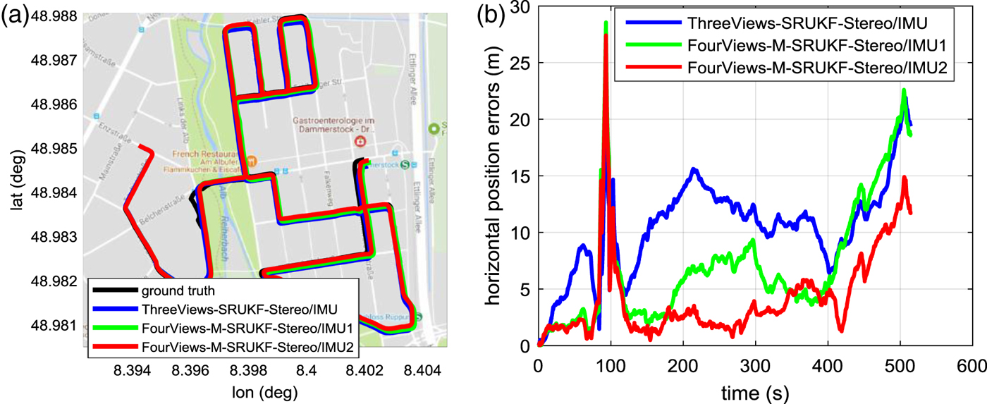
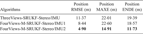
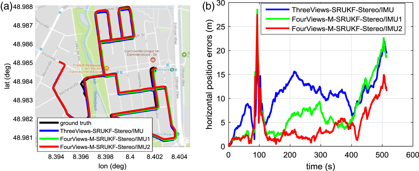
The test chosen has a trajectory of about 4.1 km (which is the longest trajectory in the dataset) and lasts 518 s with average velocity of 8 m/s. The horizontal position errors are displayed in Table 2. Note that the large error from 75 s to 120 s is caused by ground truth error due to GPS signal loss. For this reason, this period was not taken into consideration when calculating the overall Root Mean Square Error (RMSE), the Maximum Error (MAXE) and the End point Error (ENDE). Figure 4(a) and 4(b) show the estimated trajectories of different algorithms on a Google Map background and the corresponding horizontal position errors with time.
Estimated trajectories of different algorithms of the land vehicle test. (a) Trajectories on google map. (b) Horizontal positions errors of different algorithms.
Horizontal position errors of the land vehicle test
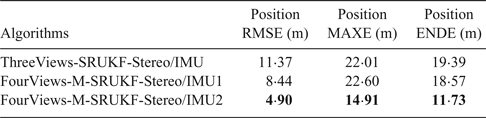
The results clearly show that the FourViews-M-SRUKF-Stereo/IMU2 has the highest positioning accuracy, with overall position error RMSE 4.90 m, MAXE 14.91 m and ENDE 11.73 m. However, the ThreeViews-SRUKF-Stereo/IMU has overall position error RMSE 11.37 m, MAXE 22.01 m and ENDE 19.39 m. The FourViews-M-SRUKF-Stereo/IMU2 has improved the accuracy by adding the quadrifocal tensor constraints. The FourViews-M-SRUKF-Stereo/IMU1 also shows higher accuracy than the ThreeViews-SRUKF-Stereo/IMU in terms of position error RMSE, but both systems have a similar MAXE accuracy. The FourViews-M-SRUKF-Stereo/IMU2 has higher accuracy than the FourViews-M-SRUKF-Stereo/IMU1. This is because the former uses more quadrifocal tensor constraints than the latter, which is more reliable for the Kalman filter measurements and the outlier rejection process.
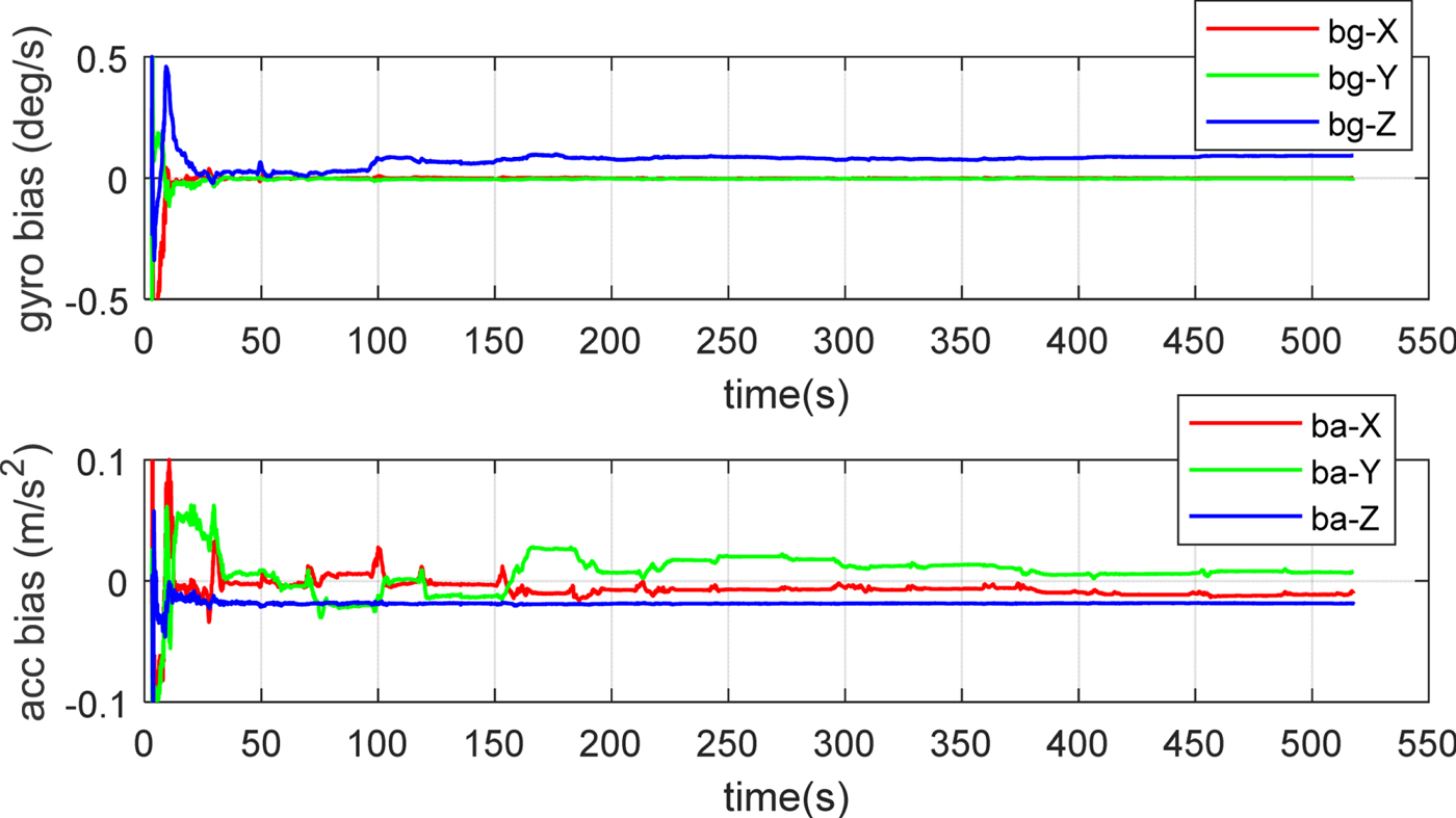
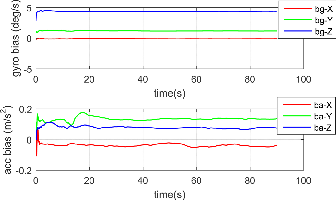
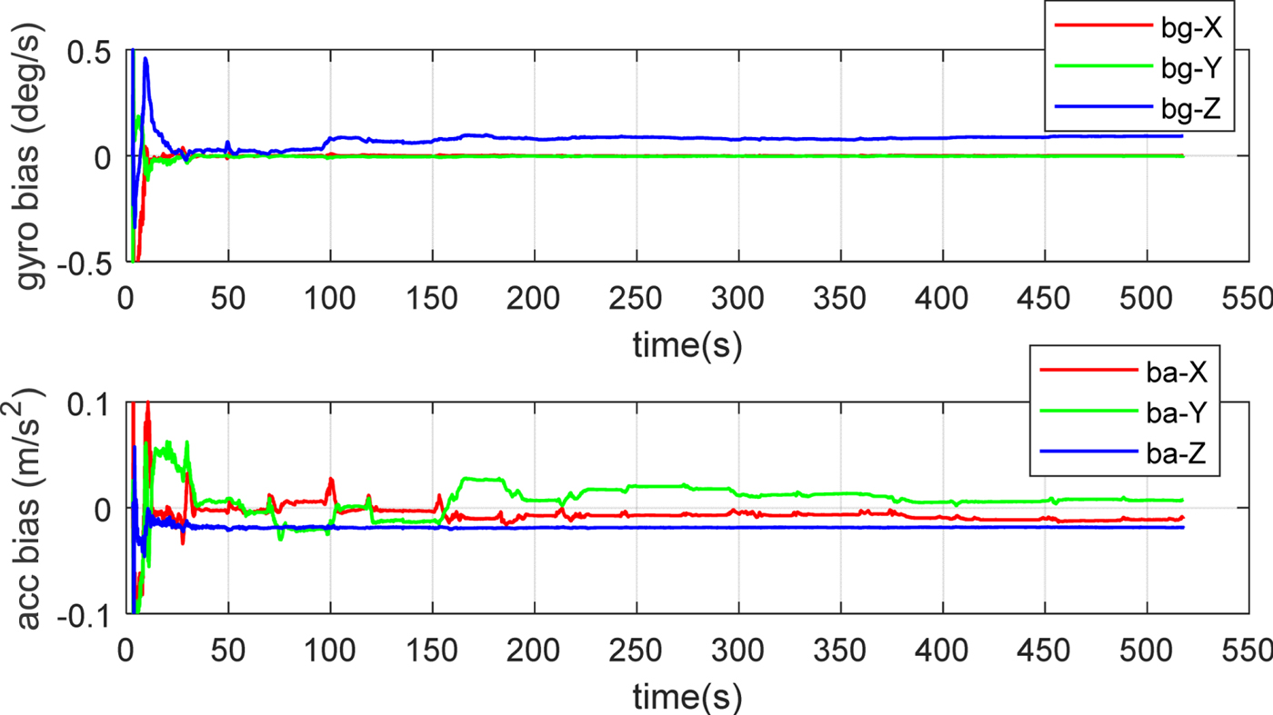
Figure 5 indicates that the new binocular vision-IMU mechanisation can estimate the gyro and the accelerometer biases successfully, which is crucial for long endurance autonomous navigation.
Estimated gyro and accelerometer biases of the land vehicle test.
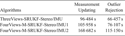
A computation load comparison among the ThreeViews-SRUKF-Stereo/IMU, the FourViews-M-SRUKF-Stereo/IMU1 and the FourViews-M-SRUKF-Stereo/IMU2 is also conducted. The computation time (by using MATLAB) of the measurement updating process and the outlier rejection process are compared.
The major differences of the two FourViews-M-SRUKF-Stereo/IMUs and the ThreeViews-SRUKF-Stereo/IMU are that the FourViews-M-SRUKF-Stereo/IMUs utilise the M-SRUKF flow which is using only n + 1 sigma points, while the ThreeViews-SRUKF-Stereo/IMU uses the standard SRUKF flow which uses 2n + 1 sigma points; the former has nearly half the computation load of the latter. However, the FourViews-M-SRUKF-Stereo/IMUs has more computation load on the Kalman filter measurements and the outlier rejection process, which can be seen from Equations (12) and (21).
The measurement updating time and outlier rejection time in Table 3 show that both the FourViews-M-SRUKF-Stereo/IMU1 and the FourViews-M-SRUKF-Stereo/IMU2 have more computation cost than the ThreeViews-SRUKF-Stereo/IMU. However, in real time application by using C + +, this is not a problem. Though the computation load of the FourViews-M-SRUKF-Stereo/IMU2 is heaviest, the accuracy improvement is promising.
Computation cost comparison

6.2. MAV test
The second dataset is from the European Robotics Challenge (EUROC) which covers the machine hall at Eidgenössische Technische Hochschule (ETH) (Burri et al., Reference Burri, Nikolic, Gohl, Schneider, Rehder, Omari, Achtelik and Siegwart2016): a typical environment to demonstrate industrial inspection using MAV. The stereo images (752 × 480) are 20 Hz, and IMU (ADIS16448, micro electro mechanical systems-MEMS) data is 200 Hz, they were all precisely synchronised. The ground truth was obtained by using a laser-tracker, which precisely measured the Three-Dimensional (3D) position by tracking a prism mounted on the MAV. A batch optimisation is employed offline, thus the six Degree of Freedom (DoF) pose in the ground truth was also provided.
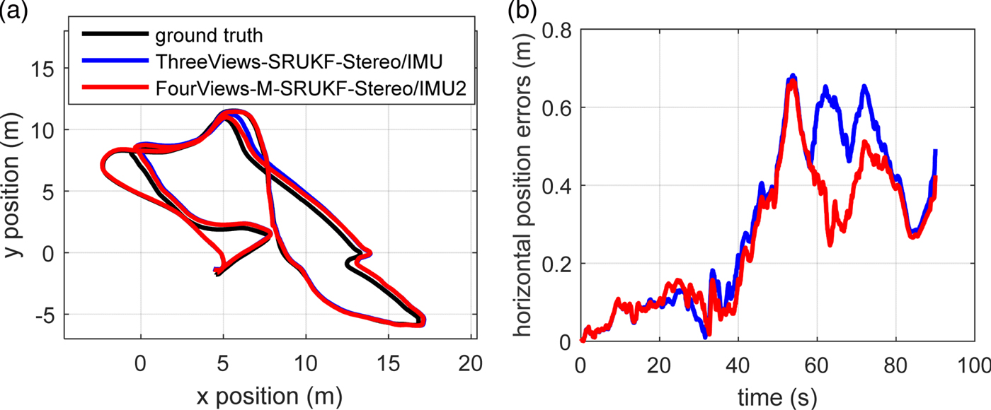
A typical case from the dataset is chosen for algorithm evaluation, which was “MH_05_diffcult”. The initial inputs of our algorithms were set from the ground truth data. The position result comparison among different algorithms is shown in Figure 6.
Estimated trajectories of different algorithms of the MAV test. (a) Top-down view of the trajectories. (b) Horizontal positions errors of different algorithms.
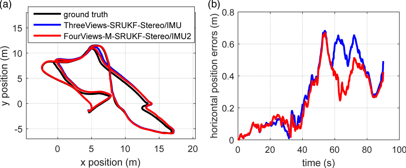
Figure 7 indicates that the new binocular vision-IMU mechanisation can estimate the gyro and the accelerometer biases successfully in the MAV test, because all the biases converge quickly to nearly constant values.
Estimated gyro and accelerometer biases of the MAV test.
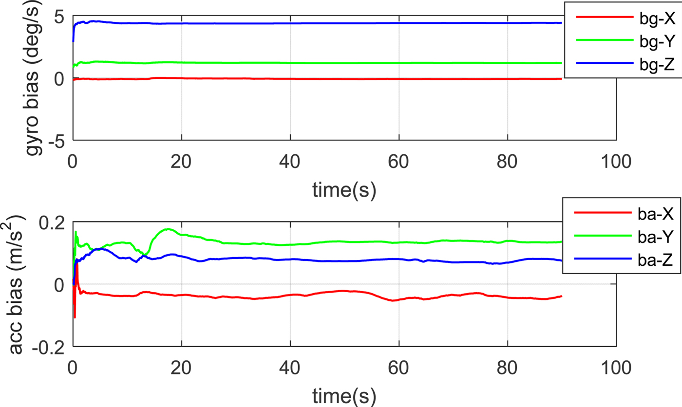
All the land vehicle and MAV test results show that the new mechanisation FourViews-M-SRUKF-Stereo/IMU2 has the best accuracy, which means that the mechanisation ThreeViews-SRUKF-Stereo/IMU by merely using the epipolar and the trifocal tensor constraints in Equation (13) is not enough to cover all the useful measurement information. However, the quadrifocal tensor constraint has the potential to provide more accurate measurement information which is not implied in both the epipolar and the trifocal tensor constraints. The quadrifocal tensor constraint has not only been used in the Kalman filter measurement model, but also used in the outlier rejection process. This implies that the extracted features are more accurate due to the addition of the quadrifocal tensor geometry constraint among four views. So, the proposed quadrifocal tensor mechanisation is an effective method to be used in the binocular vision-IMU tightly-coupled system.
7. CONCLUSIONS
In this paper, we propose a binocular vision-IMU tightly-coupled structure based on M-SRUKF for real time navigation. The reason for choosing M-SRUKF is that it has only half the sigma points of a standard SRUKF while their accuracy are nearly the same for a binocular vision-IMU tightly-coupled system. The measurement model and the outlier rejection model not only utilised the epipolar constraint and the trifocal tensor geometry constraints between the consecutive two image pairs, but also used the quadrifocal tensor geometry among four views between the consecutive times.
The experiments were carried out by using an open source KITTI dataset and a MAV dataset. Results showed that the new mechanisation (FourViews-M-SRUKF-Stereo/IMU2) worked well in both cases. In the longest land vehicle trajectory, the overall position error RMSE and MAXE were 4.90 m and 14.91 m, respectively, which is better than 11.37 m and 22.01 m by using the ThreeViews-SRUKF-Stereo/IMU. The typical case in the MAV test also shows the high position accuracy of the new mechanisation. The proposed method can greatly suppress the navigation error, so it is suitable for real time navigation, especially for GPS signal-denied environments.
ACKNOWLEDEMENT
The authors want to express their sincere thanks for the support of China Scholarship Council (CSC, File No. 201603170338).