1 Introduction
Hairpin vortices are commonly considered to be one of the major classes of coherent motion in shear layers, even as their significance in the grand scheme of turbulent flows has remained an openly debated question (e.g. Moin & Kim Reference Moin and Kim1985; Rogers & Moin Reference Rogers and Moin1987; Sayadi, Hamman & Moin Reference Sayadi, Hamman and Moin2013). The statistical prevalence of the dynamic process that gives rise to hairpins across different types of flows suggests an origin in a robust common mechanism triggered by conditions widespread in wall-bounded shear layers. This work seeks to shed light on the mechanism and characterize the conditions that drive the hairpin process. The study is primarily facilitated through an algorithm based on morphological operations which allows the identification and analysis of coherent flow processes across multiple scales. Application to data from direct numerical simulations (DNS) enables the time-resolved sampling and exploration of the hairpin process in real transitional and turbulent flow. Linear analyses provide further insight into the flow physics and especially into the connection between the hairpin process and exponential growth mechanisms.
The concept of characteristic vortices that take the form of hairpins was introduced by Theodorsen (Reference Theodorsen1952, Reference Theodorsen, Görtler and Tollmien1955) more than six decades ago. The work postulated an arc-shaped vortical structure which rises from a vortex sheet following a localized velocity fluctuation in the normal direction. Flow visualizations by Head & Bandyopadhyay (Reference Head and Bandyopadhyay1981) provided a detailed structural characterization of hairpin vortices in boundary layers at low and moderate Reynolds numbers. Perry & Chong (Reference Perry and Chong1982) described scenarios for the generation of hairpin vortices that predict a logarithmic mean profile as well as an increase of the size of the structures with distance from the wall. The outcome of their model is thus consistent with the attached-eddy hypothesis by Townsend (Reference Townsend1961) in predicting a hierarchy of structures that scale with wall distance.
Efforts to isolate specific flow processes and events from the broadband disorder of wall-bounded turbulence can be traced back to the quadrant analyses by Wallace, Eckelmann & Brodkey (Reference Wallace, Eckelmann and Brodkey1972). They sought to broaden the understanding of the sweep and ejection events identified by Corino & Brodkey (Reference Corino and Brodkey1969) and showed that both sweeps, which describe the transport of high-speed fluid towards the wall, and ejections, which describe the transport of low-speed fluid away from the wall, generally have appreciably larger time scales than motions that are characterized by the same sign of streamwise and normal fluctuations. Blackwelder & Kaplan (Reference Blackwelder and Kaplan1976) devised the VITA (variable-interval time-averaging) technique so as to obtain further insight into the structure of wall turbulence. An enhanced version of the concept, developed by Kim (Reference Kim1983), was applied by Kim & Moin (Reference Kim and Moin1986) to data generated in early numerical simulations. Their results indicated that so-called bursting events, which can be seen as powerful ejections, coincide with the emergence of hairpins.
Smith et al. (Reference Smith, Walker, Haidari and Sobrun1991) aimed to explain the formation of hairpins in wall turbulence through a detailed kinematic description. Extending their work, Zhou et al. (Reference Zhou, Adrian, Balachandar and Kendall1999) and Adrian, Meinhart & Tomkins (Reference Adrian, Meinhart and Tomkins2000) proposed a refined model which accounts for the formation of packets of hairpins, i.e. a row of structures aligned in the streamwise dimension. Pure kinematic models are nonetheless unable to provide a compelling explanation of why the wall shear statistically prefers the hairpin process compared with other realizable dynamical structures. In an extension of the earlier work, Adrian (Reference Adrian2007) aimed to connect the hairpin process to turbulent streaks which describe a second major class of coherent structures. The study postulated that a set of aligned hairpin vortices would lead to the generation of streaks in turbulent shear flow.
Not all authors agree with the notion of the hairpin process being at the origin of turbulent streaks. Studies by del Alamo et al. (Reference del Alamo, Jimenéz, Zandonade and Moser2006) identified the hairpins as a consequence of regions of low-speed fluid, while the tracking of structures in channel flow by Lozano-Durán & Jimenéz (Reference Lozano-Durán and Jimenéz2014) led to the conclusion that the hairpins may be the outcome rather than the cause of ejections of fluid away from the wall. Schlatter et al. (Reference Schlatter, Li, Örlu, Hussain and Henningson2014) took an even more critical stance by suggesting that the plethora of hairpin structures observed, for instance, in direct simulations (see, e.g., Wu & Moin Reference Wu and Moin2009) would be a trivial artefact of the relatively low Reynolds numbers, and have no significance for the dynamics within the shear layer. This view contrasts to some extent with data gained from the conditional averaging of vortical structures in turbulent boundary layers. Dennis & Nickels (Reference Dennis and Nickels2011a ,Reference Dennis and Nickels b ) identified flow structures based on the local swirling strength, and showed that while unambiguous hairpins as visualized, for example, by Adrian et al. (Reference Adrian, Meinhart and Tomkins2000) are largely absent at higher Reynolds numbers, the conditional average converges to well-defined arc-shaped structures. A characterization and classification of the hairpin process in the wider context of general coherent motion in wall-bounded shear is found in the comprehensive reviews by Robinson (Reference Robinson1991) and Smits, McKeon & Marusic (Reference Smits, McKeon and Marusic2011).
Over time, increasingly sophisticated methods have been employed with the aim of identifying and analysing flow structures in shear flows. Blackburn, Mansour & Cantwell (Reference Blackburn, Mansour and Cantwell1996) and later del Alamo & Jimenéz (Reference del Alamo and Jimenéz2006) used the discriminant criterion introduced by Chong, Perry & Cantwell (Reference Chong, Perry and Cantwell1990) to identify individual vortices as well as vortex clusters in turbulence. Marquillie, Ehrenstein & Laval (Reference Marquillie, Ehrenstein and Laval2011) extracted individual streaks from turbulent channel flow and computed a conditional average which was used as a basis for stability analyses. A similar approach was pursued by Hack & Zaki (Reference Hack and Zaki2014a
) in the context of transitional flow to demonstrate the effect of oscillatory wall forcing on the laminar streaks in bypass transition. Elsinga et al. (Reference Elsinga, Poelma, Schröder, Geisler, Scarano and Westerweel2012) tracked the evolution of vortices in a turbulent boundary layer using tomographic particle image velocimetry (PIV) data. Their results indicated that vortical structures are advected over considerable distances while maintaining their original topology. Yang & Pullin (Reference Yang and Pullin2011) applied a curvelet transform to investigate flow structures in channel flow using Lagrangian tracking. Investigations into swirling motion in two-dimensional PIV planes parallel to the walls by LeHew, Guala & McKeon (Reference Lehew, Guala and McKeon2013) showed that the convection velocity of the structures increases with wall distance. More recently, Lozano-Durán & Jimenéz (Reference Lozano-Durán and Jimenéz2014) tracked the evolution of vortical structures in turbulent channel flow by representing their spatial overlap at consecutive time instants through a graph. In this setting, the merging and splitting of structures was represented through the creation and termination of branches. At comparatively high Reynolds numbers,
 $1000\lesssim Re_{\unicode[STIX]{x1D70F}}\lesssim 4000$
, the spreading of the scales led to a flow predominantly occupied by disorganized multiscale features.
A range of studies extracted coherent structures from turbulent flows using data-based methodologies such as proper orthogonal decomposition (POD) (e.g. Bakewell & Lumley Reference Bakewell and Lumley1967; Aubry, Holmes & Stone Reference Aubry, Holmes and Stone1988). The approach generates a set of linearly independent modes which are ranked by their fluctuation energy and hierarchically describe the spatio-temporal evolution of the flow and was, for instance, applied by Moin & Moser (Reference Moin and Moser1989) to channel flow. Due to the energy ranking and the orthogonality of the modes, a large number of modes can be required in the representation of flow structures that are only weakly energetic but nonetheless contribute significantly to the overall dynamics. The dynamic mode decomposition (DMD) introduced by Schmid (Reference Schmid2010) alleviates this limitation by allowing the non-orthogonality of the modes and extracting flow features based on their single-frequency content. Application of the technique to the late stages of natural transition to turbulence demonstrated that a small number of modes can accurately reproduce the Reynolds stresses (Sayadi et al. Reference Sayadi, Schmid, Nichols and Moin2014). While DMD has proven to be an excellent tool in the study of periodic flows, including transition due to harmonic forcing, Sayadi et al. (Reference Sayadi, Schmid, Nichols and Moin2014) noted that it may be less well suited for chaotic flows that lack a well-defined peak in the frequency spectrum such as fully developed turbulence.
Aside from artificially generated flows which may represent conditions of limited relevance, the relatively undistorted and narrowband state during transition to turbulence allows perhaps the clearest view of the evolution of dynamical processes. Accounts of the affinity between the mechanisms and structures in transitional and turbulent flows can be traced back at least to the discussion of ‘transition-’ and ‘wall-layer streaks’ by Kline et al. (Reference Kline, Reynolds, Schraub and Runstadler1967) and continue to be the subject of a wide range of studies (e.g. Park et al. Reference Park, Wallace, Wu and Moin2012; Wu et al. Reference Wu, Moin, Wallace, Skarda, Lozano-Durán and Hickey2017). From a topological point of view, the turbulent hairpin bears clear similarity to the arc-shaped structures observed during the late stages of transition to turbulence. The agreement of the flow statistics collected in this region with turbulent flow led Sayadi et al. (Reference Sayadi, Hamman and Moin2013) to postulate that the late-stage transitional hairpin may serve as a low-order model of the turbulent hairpin process. An open question that we seek to address in this work is whether the transitional and turbulent hairpin processes can in fact be related to an equivalent mechanism.
A convenient aspect of transitional flows is their accessibility to linear analysis, with the early stages of natural transition in boundary layers well captured by linear stability theory (see, e.g., Herbert Reference Herbert1988). Within a range of Reynolds numbers, Blasius flow supports the amplification of a viscous exponential instability, commonly known as Tollmien–Schlichting (TS) wave. By means of parametric resonance, the TS wave can excite a three-dimensional secondary instability of fundamental or subharmonic frequency, leading to the classical scenarios of K- and H-type natural transition (Klebanoff, Tidstrom & Sargent Reference Klebanoff, Tidstrom and Sargent1962; Herbert Reference Herbert1984). While the high amplitudes during the late stages of transition enhance the significance of nonlinear effects, linear dynamics may still play an important role in advancing the flow towards turbulence.
In the realm of fully turbulent flows, a range of studies have turned to linear theory to gain insight into the underlying mechanisms that redistribute energy from the mean shear into fluctuations. As noted by Reynolds & Hussain (Reference Reynolds and Hussain1972), a fundamental complication in the application of linear analysis to averaged turbulent base flows is the necessity to include an eddy viscosity to account for the effects of small scales. This work also demonstrated that the turbulent mean is stable at moderate Reynolds numbers. The same conclusion was reached by del Alamo & Jimenéz (Reference del Alamo and Jimenéz2006), who consequently focused on the study of so-called algebraic or non-modal growth which is unrelated to the exponential stability of a flow (see, e.g., Trefethen et al. Reference Trefethen, Trefethen, Reddy and Driscoll1993; Hack & Moin Reference Hack and Moin2017). As had been shown earlier for the transitional boundary layer, algebraic growth explains the formation of streaks through the normal displacement of the mean momentum of the flow (Landahl Reference Landahl1975; Butler & Farrell Reference Butler and Farrell1992). The algebraic amplification of disturbances was pursued further by Cossu, Pujals & Depardon (Reference Cossu, Pujals and Depardon2009), who demonstrated that, consistent with the laminar boundary layer, the most amplified perturbations are streamwise vortices with zero frequency which evolve into elongated streaks. In agreement with the findings of del Alamo & Jimenéz (Reference del Alamo and Jimenéz2006) for the turbulent channel, their analysis predicts two distinct maxima for the perturbation kinetic energy, an inner extremum located within the buffer layer and a second maximum situated in the outer layer. Beyond the lift-up process, the Orr mechanism provides a second pathway for algebraic growth in shear flows (see, e.g., Farrell Reference Farrell1987). The role of the mechanism in the context of wall turbulence was contemplated by Jimenéz (Reference Jimenéz2013).
While the turbulent mean is exponentially stable in both boundary layers and channels, the presence of primary perturbations generated by algebraic mechanisms and the associated introduction of inflection points can make the flow susceptible to the amplification of secondary instabilities (see, e.g., Andersson et al. Reference Andersson, Brandt, Bottaro and Henningson2001; Hack & Zaki Reference Hack and Zaki2014b ). Recently, evidence has emerged for a possible link between linear instability mechanisms and the generation of hairpin vortices. The resolvent analysis by Sharma & McKeon (Reference Sharma and McKeon2013) showed a localization of the modes associated with very large structures in the vicinity of their critical layer based on the turbulent mean profile, suggesting the presence of an inviscid mechanism. In the context of transitional flow, Hack & Zaki (Reference Hack and Zaki2014b ) showed that the breakdown of streaks following a varicose secondary instability is accompanied by the formation of a hairpin structure.
The present work aims to characterize the transitional and turbulent hairpin processes and to shed light on the underlying mechanism that causes the recurring formation of the coherent structure in wall-bounded shear. The methodology combines the time-resolved sampling of hairpins across multiple scales with linear stability theory. This paper is structured as follows. In § 2, the flow configuration and the computational set-up used in the flow simulations are summarized. A method for investigating dynamic flow processes based on topological criteria is introduced in § 3. The results for transitional flow in § 4 cover statistical data and linear theory with focus on an individual hairpin as well as hairpin packets. The hairpin process in turbulent flow is examined in § 5 by studying both a single sample and a time-resolved conditional average. The paper ends with concluding remarks in § 6.
2 Direct numerical simulations
The flow fields used in the analysis are computed in direct numerical simulations of complete K-type transition based on the set-up described in Sayadi et al. (Reference Sayadi, Hamman and Moin2013). The simulation code solves the compressible Navier–Stokes equations in conserved variables using a spatial discretization based on fourth-order finite differences. At the considered free-stream Mach number,
 $Ma=0.2$
, compressibility effects are negligible. In the following, length scales are normalized by the distance of the inflow location from the leading edge,
 $x_{0}=1$
, and velocities are normalized by the free-stream convective velocity,
 $U_{\infty }=1$
. The viscosity is
 $\unicode[STIX]{x1D708}=1\times 10^{-5}$
and the Reynolds number at the inflow location is
 $Re_{x}=10^{5}$
. Within the turbulent region, the Reynolds number grows from
 $Re_{x}=4\times 10^{5}$
to
 $Re_{x}=9\times 10^{5}$
. In terms of the momentum thickness, the Reynolds number of the turbulent regime ranges from
 $Re_{\unicode[STIX]{x1D703}}=500$
to
 $Re_{\unicode[STIX]{x1D703}}=1500$
.
The simulations follow the experiments by Kachanov & Levchenko (Reference Kachanov and Levchenko1984) and the computations by Fasel & Konzelmann (Reference Fasel and Konzelmann1990) in triggering natural transition to turbulence through a controlled blowing and suction boundary condition at the wall at
 $1.36\leqslant x\leqslant 1.56$
. The forcing introduces a primary Tollmien–Schlichting wave with zero spanwise wavenumber and frequency
 $F=10^{6}\times \unicode[STIX]{x1D714}\unicode[STIX]{x1D708}/U_{\infty }^{2}=110$
. The three-dimensionality required for the eventual breakdown to turbulence is provided by a temporally fundamental oblique mode with spanwise wavenumber
 $\unicode[STIX]{x1D6FD}=2\unicode[STIX]{x03C0}/\unicode[STIX]{x1D706}=41.88$
, which is also introduced through the wall forcing. The TS wave is exponentially unstable at the considered Reynolds number and is amplified during the initial stage of the transition process. Its presence modulates the base flow and makes it eventually unstable to the amplification of the oblique mode which can therefore be interpreted as a secondary instability.
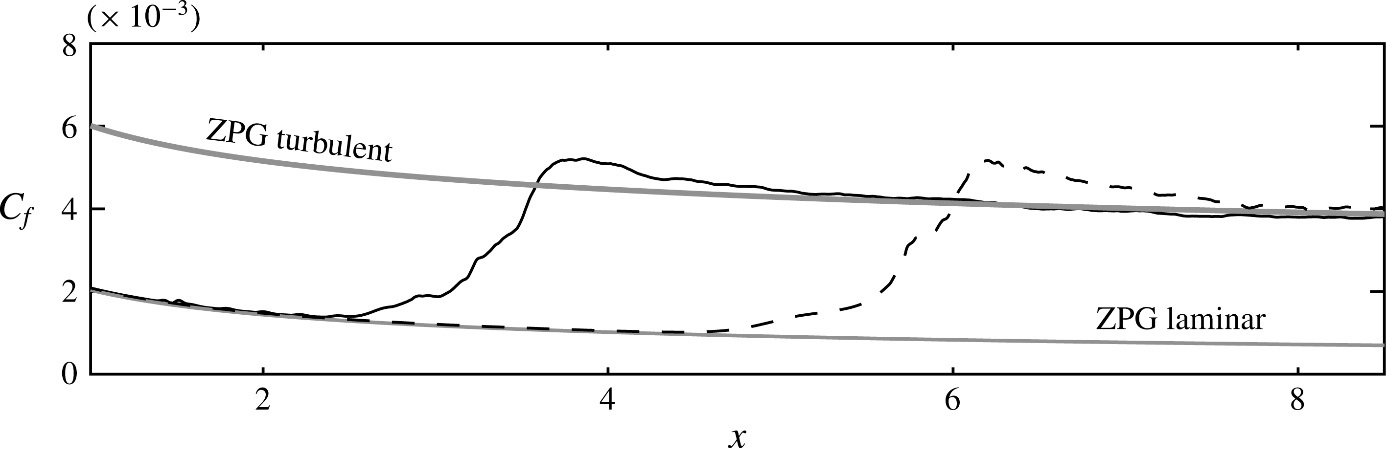
The skin-friction coefficient is presented in figure 1. The fundamental K-type case is characterized by a relatively rapid transition process, and the skin-friction curve begins to depart from the Blasius solution at
 $x\approx 2.5$
, corresponding to a Reynolds number of
 $Re_{x}=2.5\times 10^{5}$
. Also shown for reference is the subharmonic H-type breakdown, which is considerably slower, with transition initiated at
 $x\approx 4.5$
. In both cases, a characteristic overshoot of the skin-friction curves beyond the turbulent correlation is observed. Statistical results indicate that the properties of the flow at this point are largely the same as in the turbulent flow farther downstream; see Sayadi et al. (Reference Sayadi, Hamman and Moin2013).
The skin-friction coefficient of the K-type (solid) and H-type (dashed) simulations. Turbulent correlation from White (Reference White2005).

3 Time-resolved analysis of flow processes
The methodology for the analysis of flow structures presented in the following makes use of concepts introduced in the field of computer vision. Through a set of morphological operations, the structure of the flow field is distilled into a discrete graph. The approach enables the identification and time-resolved sampling of coherent processes across multiple scales based on topological criteria.
3.1 Morphological thinning
Morphological thinning compresses the geometric information contained in a general binary image by extracting the medial axes of objects. In three-dimensional Euclidean space, the medial axis of a geometry is defined as the locus of the centres of all inscribed maximal spheres of the object where these spheres touch the boundary at more than one point (see, e.g., Lam, Lee & Suen Reference Lam, Lee and Suen1992). Our method adapts the general concept presented by Lee & Kashyap (Reference Lee and Kashyap1994) to the present setting. An arbitrary geometry is represented in a discrete three-dimensional binary space
 $Z=[0,i_{max}]\times [0,j_{max}]\times [0,k_{max}]$
. Objects are described by the subset
 $S\in Z$
, which consists of all points, or voxels,
 $v$
with value 1. The empty environment is represented by the complement
 $\overline{S}$
, which contains all voxels with value 0.
The medial axis of an object is generated through the successive removal of voxels located at the object surface by setting their values to zero. Surface points are removed only if their absence does not change the topology. In formal terms, the preservation of the topology can be represented in terms of the Euler characteristic,
 $$\begin{eqnarray}G(S)\equiv O(S)-K(S)+C(S),\end{eqnarray}$$
where
 $O(S)$
is the number of objects,
 $K(S)$
is the number of holes and
 $C(S)$
is the number of cavities in
 $S$
. In contrast to cavities, holes are not entirely surrounded by
 $S$
. An equivalent formulation to (3.1) which is tailored to a digital context and the representation of objects on discrete grids is (Morgenthaler Reference Morgenthaler1981; Kong & Rosenfeld Reference Kong and Rosenfeld1989)
 $$\begin{eqnarray}H(S)\equiv n_{v}-n_{e}+n_{f}-n_{o},\end{eqnarray}$$
where
 $n_{v}$
,
 $n_{e}$
,
 $n_{f}$
and
 $n_{o}$
respectively denote the number of vertices, edges, faces and octants (i.e.
 $2\times 2\times 2$
cubes) in the set of non-zero points
 $S$
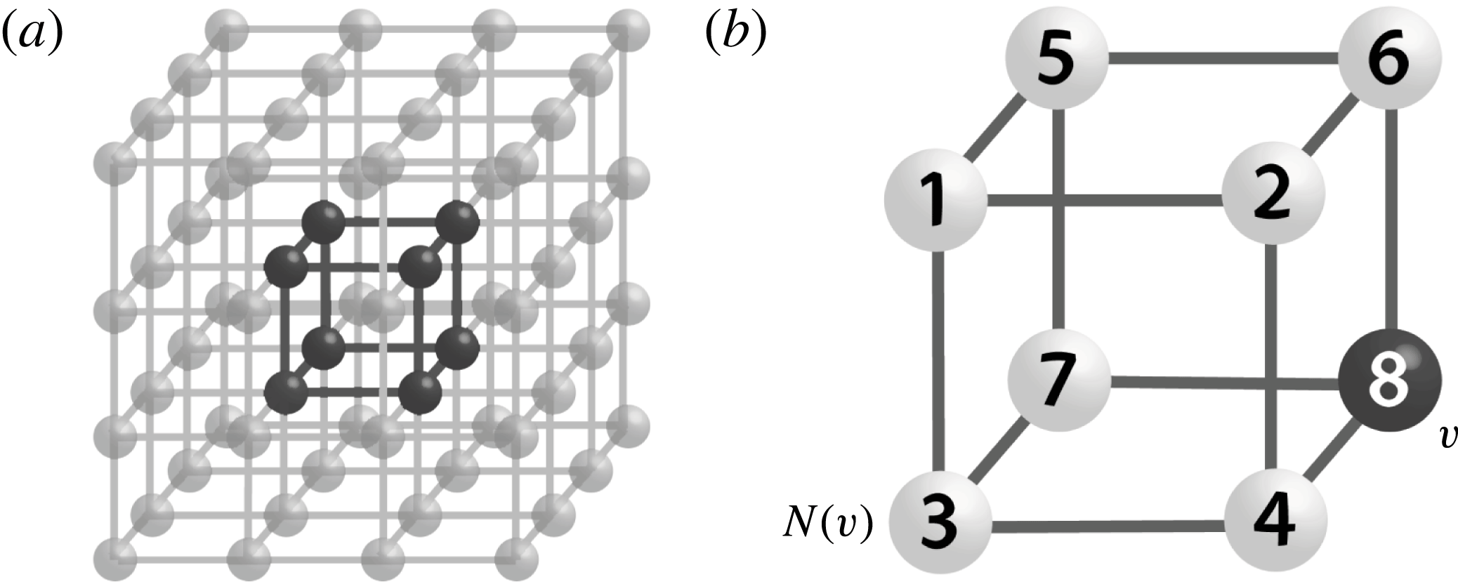
. As an example, the cube represented in figure 2(a) corresponds to
 $G(S)=1-0+0=1$
. Evaluation of the digital formulation equivalently yields
 $H(S)=8-12+6-1=1$
.
(a) Sample representation of a cube in the digital grid. (b) The octant neighbourhood
 $N(v)$
of the point
 $v$
.

In the case of large topologies, the global evaluation of (3.2) can become cumbersome. Splitting of the grid into a set of overlapping octants allows the local evaluation of the Euler characteristic in the eight-point neighbourhood
 $N(v)$
of a point
 $v$
, as visualized in figure 2(b),
 $$\begin{eqnarray}H_{l}(S\cap N(v))=\frac{n_{v,l}}{8}-\frac{n_{e,l}}{4}+\frac{n_{f,l}}{2}-n_{o,l},\end{eqnarray}$$
where
 $n_{v,l}$
,
 $n_{e,l}$
,
 $n_{f,l}$
and
 $n_{o,l}$
respectively are the local number of vertices, edges, faces and octants in
 $S\cap N(v)$
. The Euler characteristic of the full topology is calculated as the sum of the local characteristics (Lobregt, Verbeek & Groen Reference Lobregt, Verbeek and Groen1980),
 $$\begin{eqnarray}H(S)=\mathop{\sum }_{l}H_{l}.\end{eqnarray}$$
A necessary but insufficient criterion for topological preservation is the invariance of the Euler characteristic while removing points. Specifically, when removing the point
 $v$
, the variation in
 $H_{l}$
becomes
 $$\begin{eqnarray}\unicode[STIX]{x1D6FF}H_{l}=-\frac{1}{8}-\frac{\unicode[STIX]{x1D6FF}n_{e,l}}{4}+\frac{\unicode[STIX]{x1D6FF}n_{f,l}}{2}-\unicode[STIX]{x1D6FF}n_{o,l}.\end{eqnarray}$$
The computationally efficient evaluation of (3.5) exploits the limited number of
 $2^{8-1}=128$
permutations in the octant neighbourhood
 $N(v)$
which permits the generation of a lookup table of
 $\unicode[STIX]{x1D6FF}H_{l}$
for all possible permutations. Following Morgenthaler (Reference Morgenthaler1981), a complete characterization of topological preservation is achieved by additionally requiring that locally
 $\unicode[STIX]{x1D6FF}H_{l}(S\cap N(v))=0$
or
 $\unicode[STIX]{x1D6FF}O(S\cap N(v))=0$
.
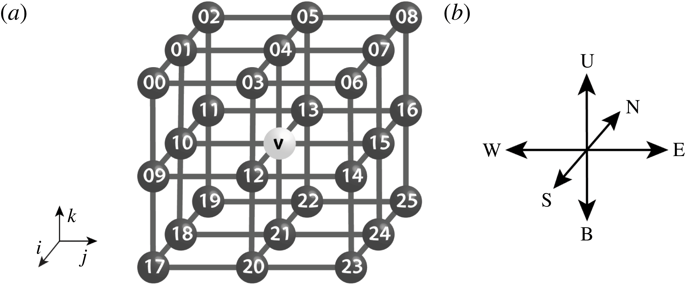
Further constraints are necessary to avoid the elimination of an object when performing the thinning operation in parallel. Each thinning step is divided into six subcycles based on the type of a border point (N, S, W, E, U or B), corresponding to cubic indices of 13, 12 10, 15, 4 and 21 (see figure 3). Doing so, however, does not entirely prevent the removal or splitting of objects. In the present implementation, the topology is preserved by sequentially verifying the connectivity of each point. Let
 $R$
denote the voxels labelled for removal during a substep, and
 $Q=S-R$
, then
 $v\in R$
is removed if points in
 $R\cap N(v)$
and
 $Q\cap N(v)$
are still connected, which is equivalent to requiring that
 $O(\{R\cap N(v)\}\cup \{Q\cup N(v)\})=1$
.
The 26-point neighbourhood of a point
 $v$
in the digital image with coordinate system.

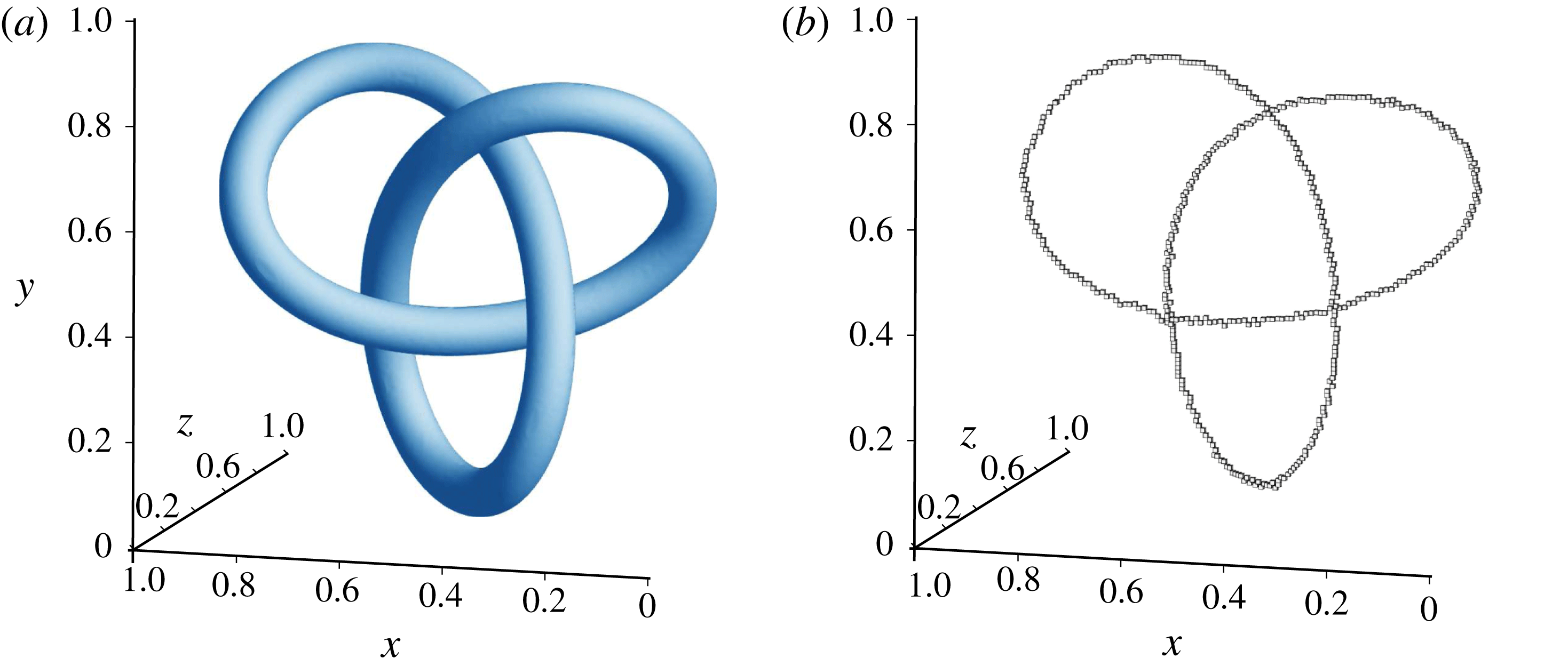
The outcome of the thinning procedure is demonstrated by applying the algorithm to a test geometry. A trefoil knot is generated on a grid of size
 $[0,1]\times [0,1]\times [0,1]$
using a resolution of
 $128\times 128\times 128$
points. Voxels within a distance of 0.05 from the curve are set to one with the remainder initialized to zero. An isosurface at
 $Z=0.5$
is shown in figure 4(a). The thinning procedure appreciably compresses the topological information by removing more than 99 % of the voxels that make up the geometry. The resulting medial line is shown in figure 4(b). It is worth pointing out that while the sample geometry is generated on a uniform grid, the thinning algorithm does not rely on grid isotropy. As such, it can be immediately applied to data represented on anisotropic computational grids as commonly used in the numerical simulation of shear layers.
Application of the morphological thinning algorithm to reference topology. (a) Binary image with isosurface at
 $Z=0.5$
. (b) Voxels representing the medial axis.

3.2 Graph generation and capture of flow structures
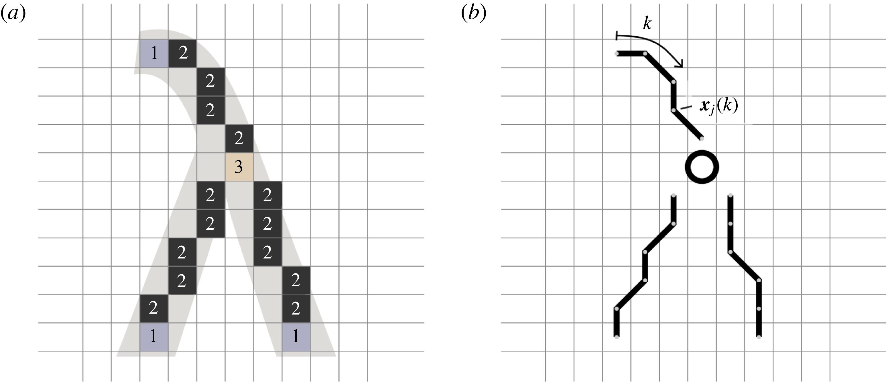
While the medial axis representation appreciably reduces the information required to describe the topology, the binary voxel image is unsuited for the algorithmic identification of structures. The starting point towards this objective is the generation of a parametric description of the geometry by transforming the network of medial axes into a discrete graph. In a first step, the connectivity of the voxels representing the objects is evaluated as visualized in figure 5 for a two-dimensional example. Numbers within each of the axis voxels indicate the total of non-zero points within the eight-point (26-point in three dimensions) neighbourhood of each voxel. Voxels with more than two neighbours, i.e. with more than two non-zero voxels in their neighbourhood, are defined as nodes.
Voxels of connectivity one and two make up the elements of links. By running along the
 $j$
th link, the grid coordinates
 $\boldsymbol{x}_{j}(k)$
of the constituting voxels are classified and stored as a function of the integer parameter
 $k$
. Finally, the start and end nodes of each link are evaluated and stored. Isolated voxels that are not connected to any other point are discarded. Furthermore, links that are only connected to one node are discarded when their length is below a prescribed threshold set at the expected minimum extent of the flow structures of interest.
Graph generation from medial axis. (a) Connectivity of the medial axis voxels. (b) Graph with links and node.

The application of the above-described algorithm to a three-dimensional flow field condenses the structure of the flow field into databases of nodes and links. Specific classes of flow features can be identified and isolated based on their topology by filtering the databases using topological criteria that can be prescribed in absolute or relative terms. An absolute criterion could, for instance, require the extent of a structure in a certain dimension to be within a given range, while a relative topological criterion could specify the extent in one dimension to be larger than that in another. The possibility of prescribing relative criteria makes the approach scale-independent and allows the identification of topologically similar structures across multiple scales.
When applying the algorithm to the three-dimensional field described by the
 $Q$
criterion (Hunt, Wray & Moin Reference Hunt, Wray and Moin1988),
 $$\begin{eqnarray}Q=-\frac{1}{2}\frac{\unicode[STIX]{x2202}u_{i}}{\unicode[STIX]{x2202}x_{j}}\frac{\unicode[STIX]{x2202}u_{j}}{\unicode[STIX]{x2202}x_{i}},\end{eqnarray}$$
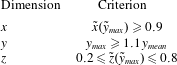
the criteria listed in table 1 gave physically meaningful results in the identification of hairpin structures, with weak sensitivity of the sampled results to changes in the filter. The criteria are expressed in terms of the scaled coordinates
 $\tilde{x}$
,
 ${\tilde{y}}$
and
 $\tilde{z}$
, which are normalized by the instantaneous bounding box of the flow structure under consideration such that
 $\tilde{x}\times {\tilde{y}}\times \tilde{z}\in [0,1]\times [0,1]\times [0,1]$
. Specifically, the first and third criteria state that the location where the computed medial axis of the flow structure attains its largest distance from the wall should be close to the downstream end of the bounding box and within a region around the spanwise centre of the bounding box. The criterion for the normal coordinate is formulated in physical coordinates and requires a certain prominence of the hairpin tip in specifying that the maximum normal distance has to be larger than 1.1 times the average value of
 $y$
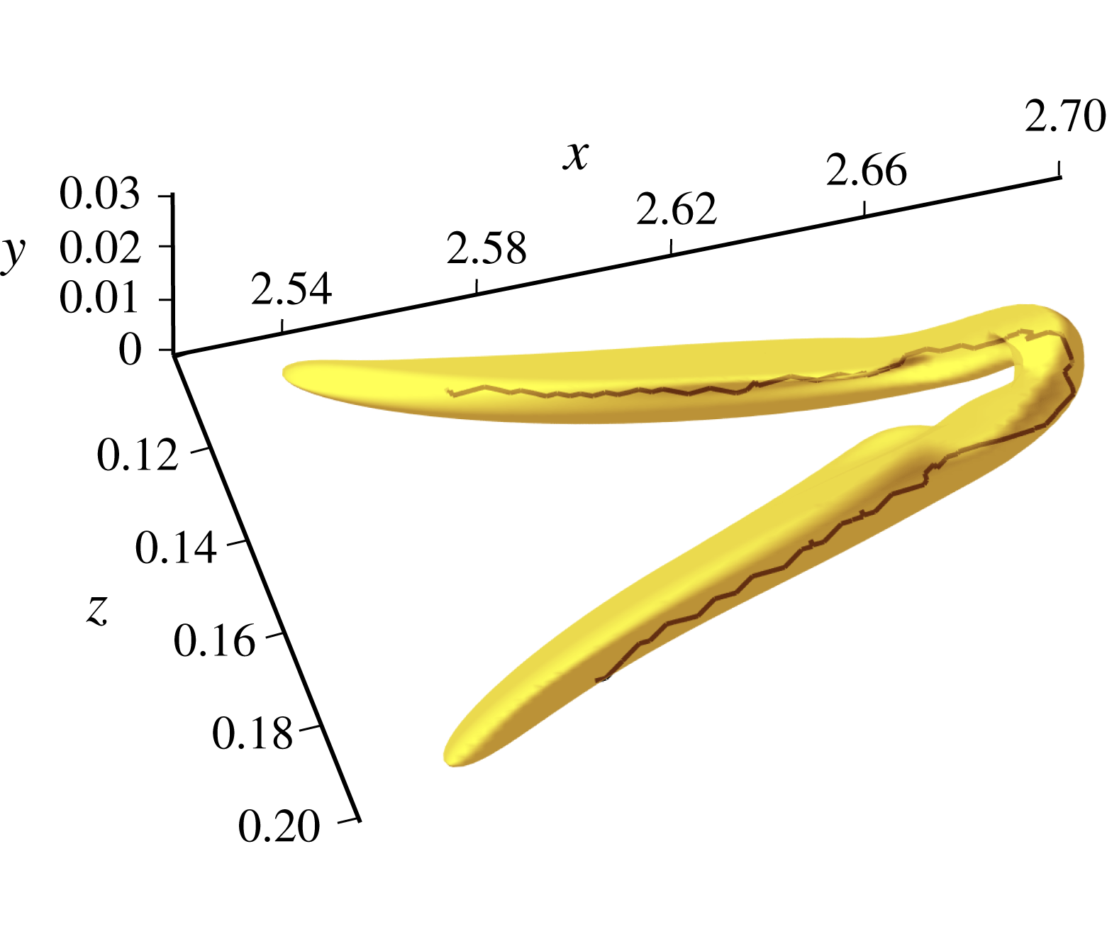
along the full medial axis of the considered structure. An isolated hairpin structure is visualized in physical coordinates in figure 6. The link generated from the medial axis line is shown in black.
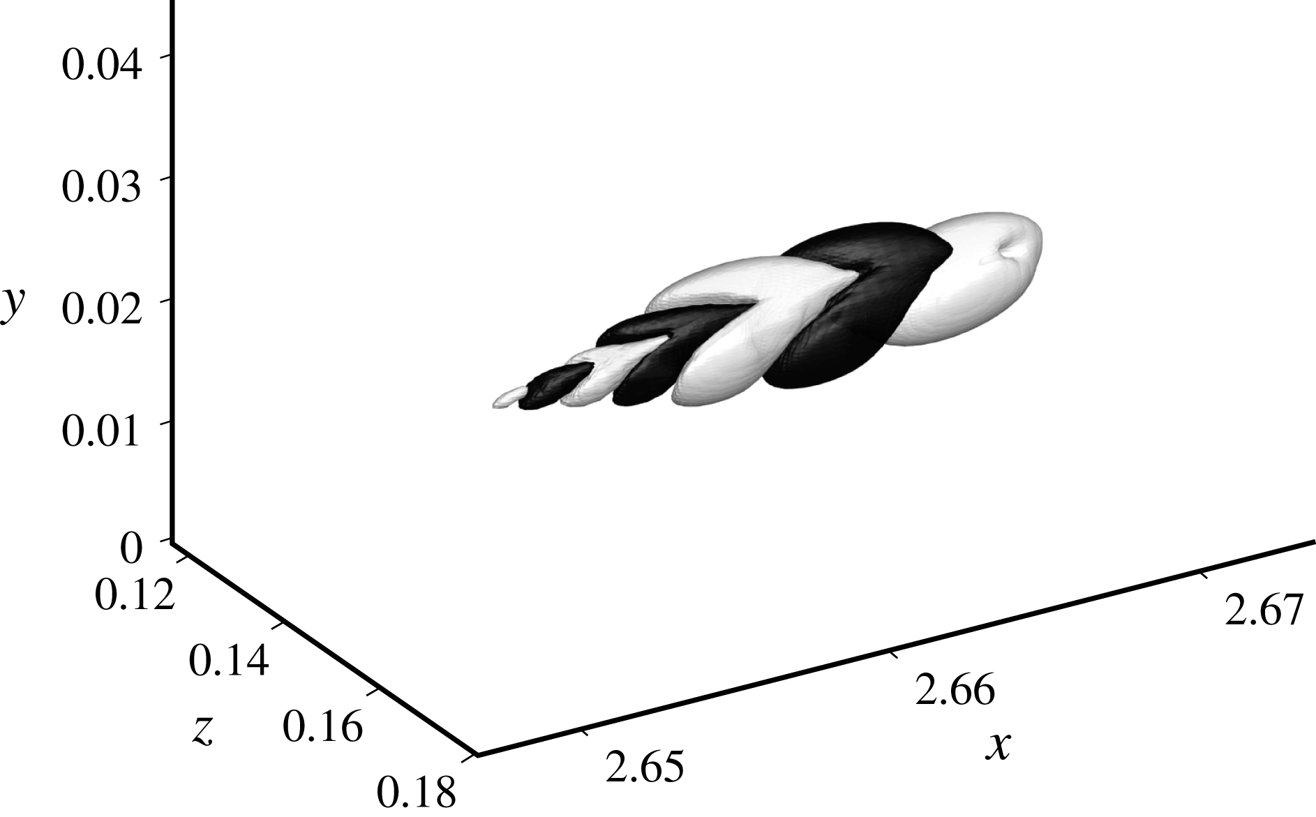
Isolated hairpin vortex from the late stage of K-type transition (isosurface of the
 $Q$
criterion) with medial axis link (black line).

The topological filtering criteria applied in the identification of the hairpin process.

The analysis of dynamic processes builds on the static identification described above. The evolution of a specific flow structure is traced as it travels through the flow field by applying the identification method to successive snapshots of a time series. The convective effect of the mean flow is incorporated by correcting the position with the local instantaneous velocity at the centre of the structure, multiplied by the time step between two consecutive flow fields,
 $\unicode[STIX]{x0394}x_{conv}=u\unicode[STIX]{x0394}t$
. Spatial overlap of the medial axes of two structures at consecutive time instants in conjunction with comparable topology implies that they are representations of the same flow feature and thus have the same label attached. The outcome of this process is a database that contains the coordinates of each structure as a function of the solution time of the simulation. A general advantage of the above method is the computerized and thus automated identification of structures through unbiased criteria. As such, it can enable statistical relevance by studying large numbers of samples of dynamical flow processes while preserving the underlying temporal causality.
4 Transitional flow
The late stages of natural transition to turbulence are characterized by the formation of hairpin vortices with length scales of the order of the boundary layer thickness. When transition to turbulence is triggered by well-defined conditions such as those corresponding to the classical K- and H-type scenarios, the outcome is a spatially separated sequence of hairpins which allows the detailed study of individual samples. In this setting, the hairpin process is initiated naturally by the modulation of the flow due to preceding primary and secondary instabilities as opposed to being forced by artificial conditions which may be irrelevant in real flows. In this section, we characterize the evolution of an individual transitional hairpin and we investigate the link to classical stability theory through linear analysis. Finally, the generation of hairpin packets in the transitional regime is examined.
4.1 Transitional hairpin
In the following, the evolution of an individual transitional hairpin is studied by applying the identification method described in § 3. The late stages of the K-type transitional region are considered,
 $2.4\times 10^{5}\lesssim Re_{x}\lesssim 3.0\times 10^{5}$
. Vortical structures can be visualized, for instance, through the vortex surface field method (e.g. Yang et al.
Reference Yang, Zaho, Xiong, Hack and Kim2016) or the
 $Q$
criterion equation (3.6), which is used throughout this work. It is worth noting that the consideration of the medial axes of the structures in the identification algorithm appreciably reduces the sensitivity with respect to the chosen
 $Q$
threshold. Furthermore, the actual hairpin is considered only as an indicator, with evaluations focusing on physical quantities such as velocity fluctuations. To this aim, the instantaneous velocity field,
 $\boldsymbol{u}(x,y,z,t)=(u,v,w)^{\text{T}}$
, is separated into a temporal and spanwise mean,
 $\overline{\boldsymbol{u}}(x,y)$
, and a fluctuation component,
 $\boldsymbol{u}^{\prime }(x,y,z,t)$
,
 $$\begin{eqnarray}\boldsymbol{u}=\overline{\boldsymbol{u}}+\boldsymbol{u}^{\prime }.\end{eqnarray}$$
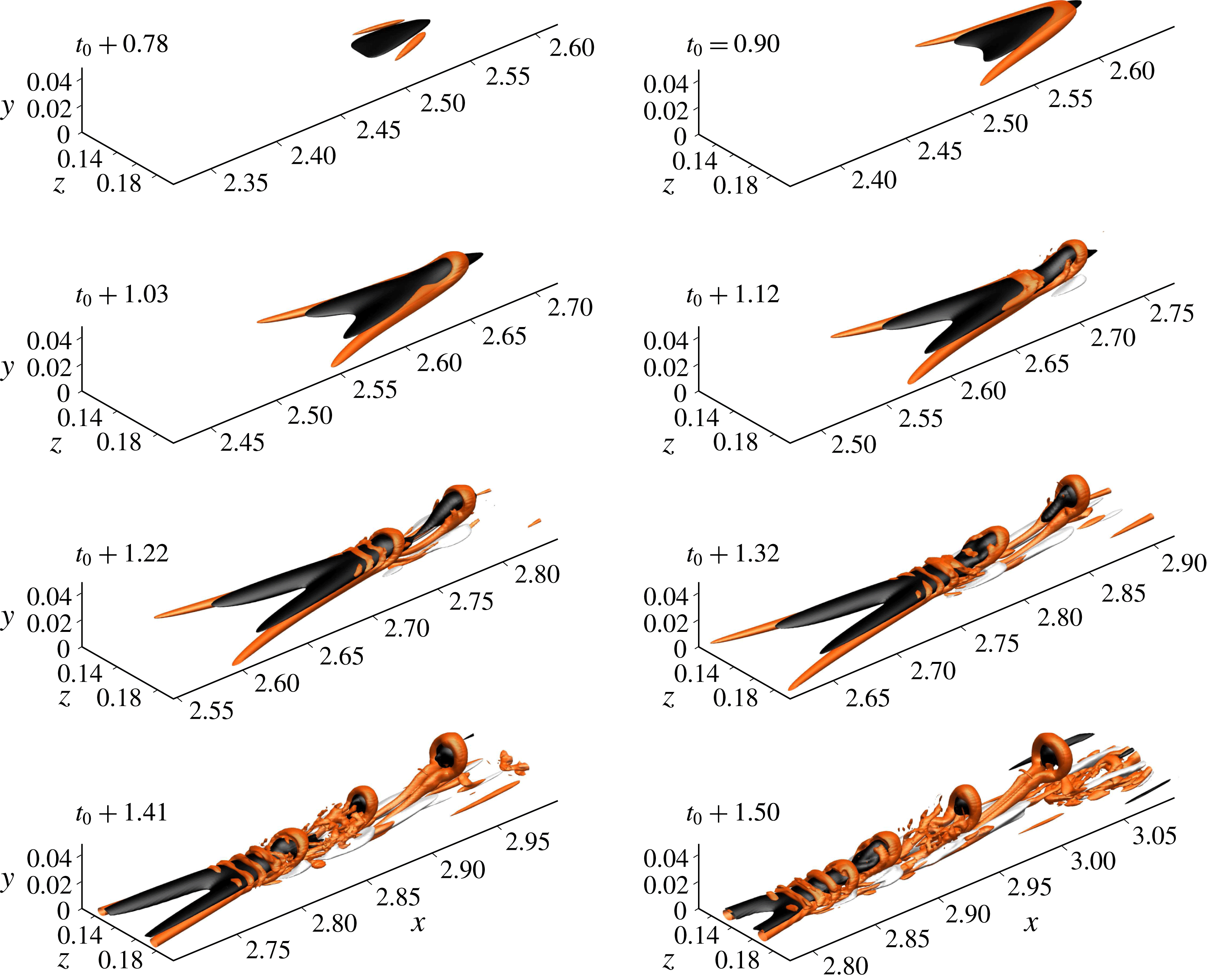
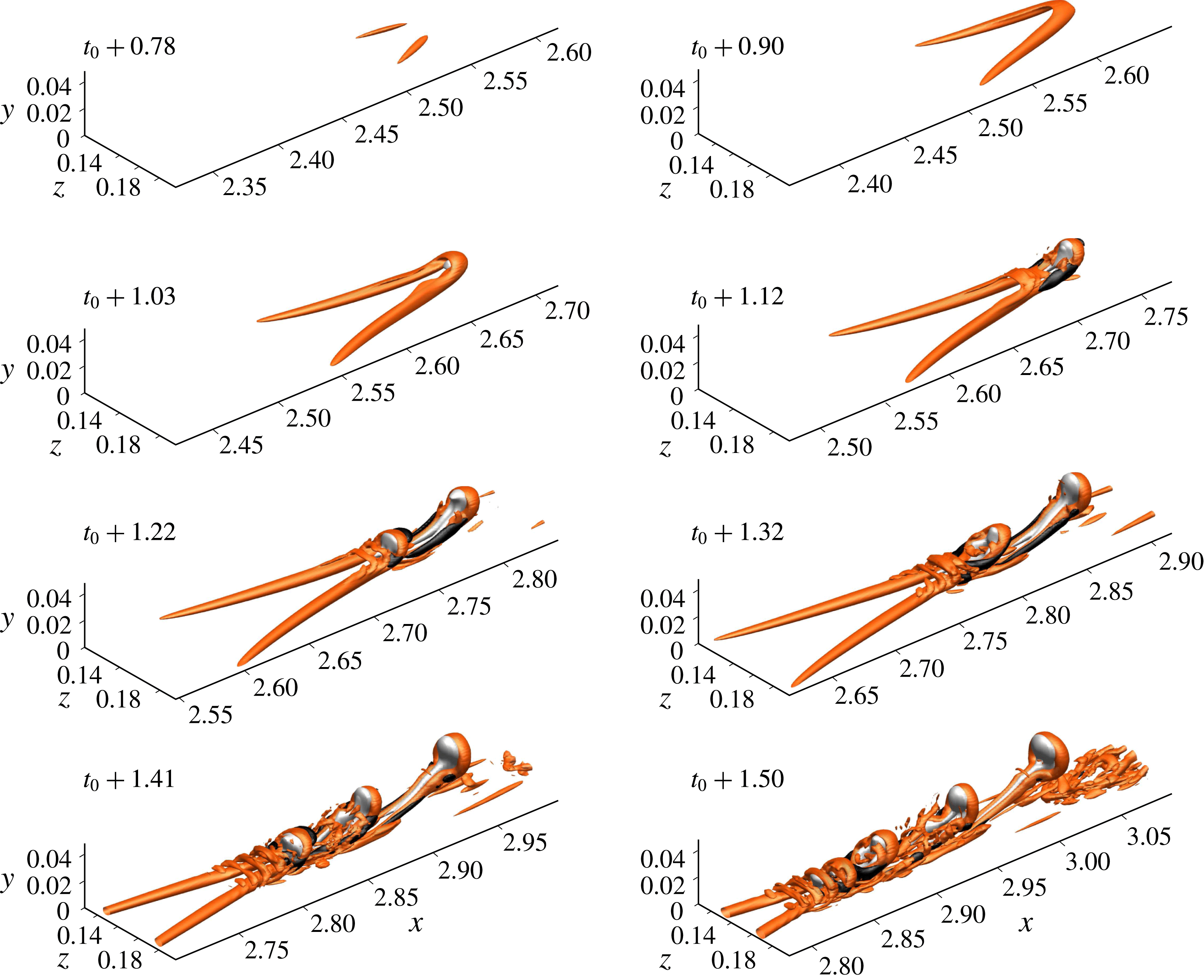
A time sequence showing the temporal evolution of a hairpin in late-stage transition is presented in figure 7. Black and white isosurfaces respectively represent negative and positive streamwise velocity fluctuations. The visualization shows that the arch of the hairpin delimits an area of low-speed fluid whose intensity increases with time. In the fourth frame, at time
 $t_{0}+1.12$
, a secondary hairpin has formed upstream of the primary structure which begins to separate from the patch of low-speed fluid. The intensity of the detached region of low-momentum fluid associated with the primary hairpin decays and is in the last two frames confined to the centre of the hairpin tip. By time
 $t_{0}+1.41$
, the second hairpin also begins to separate from the remaining patch while a third hairpin is formed.
Time series of hairpin formation during the late stage of K-type transition. Isosurfaces of
 $u^{\prime }=0.20$
(white),
 $u^{\prime }=-0.20$
(black) and
 $Q=5$
(red). An animation is available in movie 1 of the supplementary material at https://doi.org/10.1017/jfm.2018.202.

Visualizations of the wall-normal velocity fluctuations shown in figure 8 indicate that the intensity is highest at the tips of the hairpins. The shape of the area of positive
 $v^{\prime }$
fluctuations coincides with the hairpin structure in the
 $Q$
field. In general, positive normal fluctuations largely mirror the behaviour of the negative streamwise component during the separation of the primary and secondary hairpins and the formation of new structures.
Time series of hairpin formation during the late stage of K-type transition. Isosurfaces of
 $v^{\prime }=0.05$
(white),
 $v^{\prime }=-0.05$
(black) and
 $Q=5$
(red). An animation is available in movie 2 of the supplementary material.

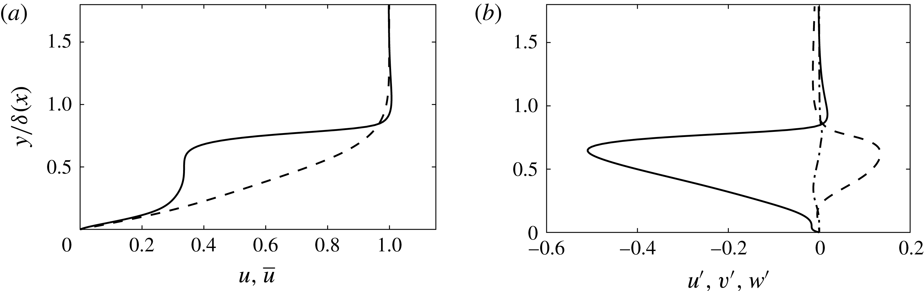
The tip of the hairpin coincides with a distinctly localized peak in the velocity fluctuations which describes the global maximum in the intensity of fluctuations within the simulation domain including the laminar and turbulent regimes. The amplitude of the distortion underlines the peculiar conditions during the late stages of transition which are also reflected in the characteristic overshoot of the skin-friction curve above the turbulent correlation (figure 1). The normal instantaneous streamwise velocity profile through the hairpin tip, at
 $x=2.66$
,
 $z=0.15$
and
 $t=t_{0}+1.03$
(third frame of the time series in figure 7), is compared in figure 9(a) with the local mean flow profile. The high intensity of the distortion locally reduces the instantaneous normal velocity gradient close to zero. The comparison of the fluctuations in all three dimensions provided in figure 9(b) shows that the magnitude of the streamwise component peaks at approximately 50 % of the free-stream velocity whereas the normal fluctuations reach a maximum of approximately 15 %. This extreme growth of the fluctuation amplitudes is likely to be a representation of the late-transitional ‘spikes’ first reported in the classical experiments by Klebanoff et al. (Reference Klebanoff, Tidstrom and Sargent1962).
Velocity profiles at the centre of the hairpin at
 $x=2.66$
,
 $z=0.15$
and
 $t=t_{0}+1.03$
. (a) Local mean (solid) and instantaneous streamwise velocity. (b) Streamwise (solid), normal (dashed) and spanwise (dash-dotted) velocity fluctuations.

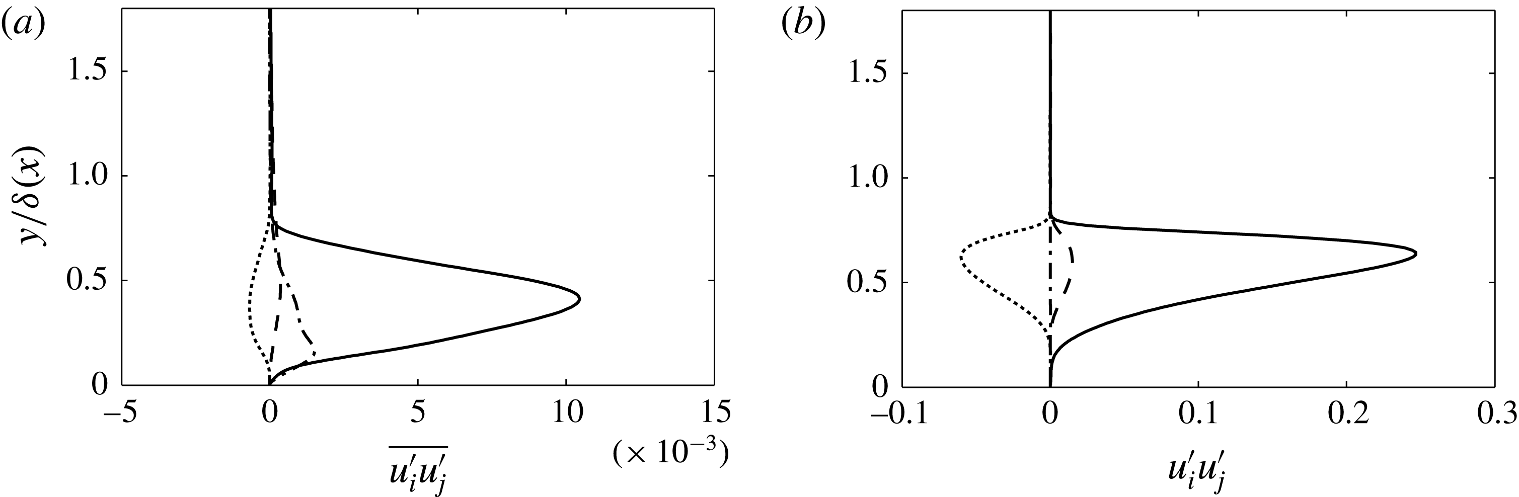
Profiles of the time- and spanwise-averaged Reynolds stresses,
 $\overline{u_{i}^{\prime }u_{j}^{\prime }}$
, at the location of the hairpin head are compared in figure 10 with the instantaneous values
 $u_{i}^{\prime }u_{j}^{\prime }$
at the instant of highest streamwise fluctuation,
 $t=t_{0}+1.03$
. The peak amplitude of the diagonal streamwise component instantaneously exceeds the maximum of the average by more than an order of magnitude. A similar behaviour is seen for the mixed component
 $u^{\prime }v^{\prime }$
. Due to the spanwise symmetry of the hairpin with respect to its centreline, the spanwise component of the Reynolds stress tensor,
 $w^{\prime }w^{\prime }$
, remains instantaneously at a relatively low level.
Profiles of the Reynolds stresses at the centre of the hairpin
 $x=2.66$
,
 $z=0.15$
and
 $t=t_{0}+1.03$
:
 $u^{\prime }u^{\prime }$
(solid),
 $v^{\prime }v^{\prime }$
(dashed),
 $w^{\prime }w^{\prime }$
(dash-dotted) and
 $u^{\prime }v^{\prime }$
(dotted). (a) Temporal and spanwise mean. (b) Instantaneous.

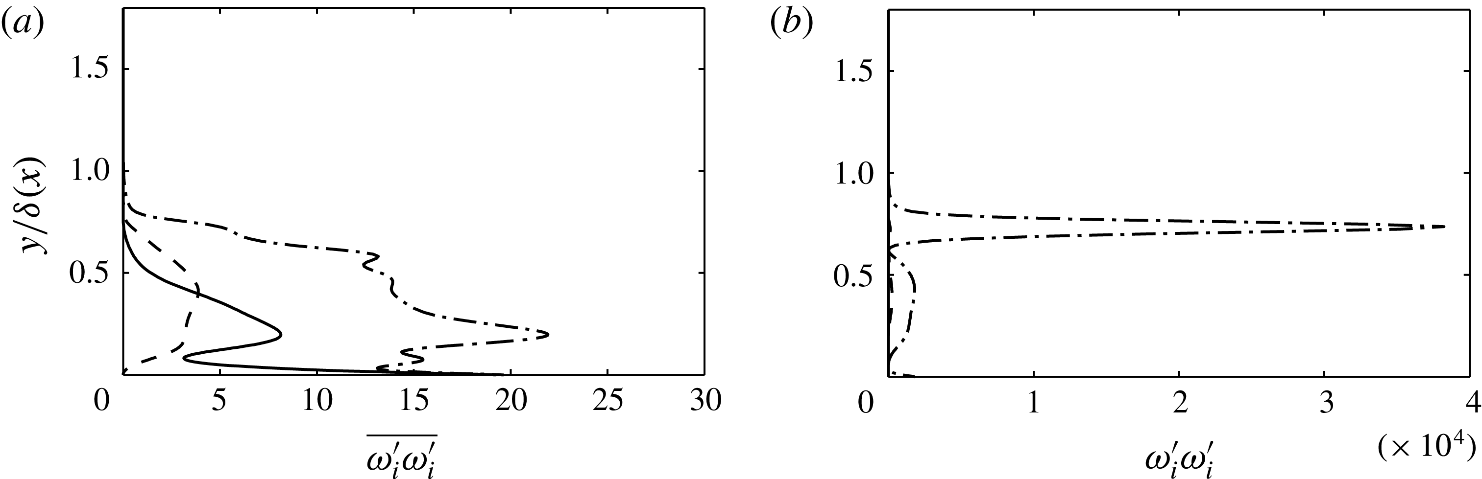
The individual terms of the enstrophy,
 $\unicode[STIX]{x1D714}^{2}\equiv \unicode[STIX]{x1D714}_{i}^{\prime }\unicode[STIX]{x1D714}_{i}^{\prime }$
, i.e. the square of the components of the fluctuation vorticity vector
 $\unicode[STIX]{x1D74E}^{\prime }=\unicode[STIX]{x1D735}\times \boldsymbol{u}^{\prime }$
, are presented in figure 11. The average shows comparable amplitudes for all three terms while, instantaneously, the appreciable momentum deficit observed at the head of the hairpin and the sharp gradient near the edge of the boundary layer result in a localized peak in the instantaneous
 $\unicode[STIX]{x1D714}_{z}^{\prime }\unicode[STIX]{x1D714}_{z}^{\prime }$
. It follows that at
 $t_{0}+1.03$
, the contribution of the spanwise component makes up more than 99 % of the total enstrophy.
Profiles of the enstrophy terms at the centre of the hairpin
 $x=2.66$
,
 $z=0.15$
and
 $t=t_{0}+1.03$
. Streamwise (solid), normal (dashed) and transverse (dash-dotted) components. (a) Temporal and spanwise mean. (b) Instantaneous.

Finally, the terms of the energy budget at the head of the hairpin are considered. Instantaneously, the rate of change of the kinetic energy in the velocity fluctuations,
 $k^{\prime }=u_{i}^{\prime }u_{i}^{\prime }/2$
, of an incompressible fluid is governed by the Reynolds–Orr equation,
 $$\begin{eqnarray}\frac{\unicode[STIX]{x2202}k^{\prime }}{\unicode[STIX]{x2202}t}=\underbrace{-u_{i}^{\prime }u_{j}^{\prime }\frac{\unicode[STIX]{x2202}\overline{u}_{i}}{\unicode[STIX]{x2202}x_{j}}}_{{\mathcal{P}}^{\prime }}-\underbrace{\frac{1}{Re}\frac{\unicode[STIX]{x2202}u_{i}^{\prime }}{\unicode[STIX]{x2202}x_{j}}\frac{\unicode[STIX]{x2202}u_{i}^{\prime }}{\unicode[STIX]{x2202}x_{j}}}_{{\mathcal{D}}^{\prime }}-\frac{1}{2}\frac{\unicode[STIX]{x2202}u_{i}^{\prime }u_{i}^{\prime }u_{j}^{\prime }}{\unicode[STIX]{x2202}x_{j}}-\frac{1}{2}\overline{u}_{j}\frac{\unicode[STIX]{x2202}u_{i}^{\prime }u_{i}^{\prime }}{\unicode[STIX]{x2202}x_{j}}-\frac{\unicode[STIX]{x2202}u_{i}^{\prime }p^{\prime }}{\unicode[STIX]{x2202}x_{i}}+\frac{1}{2}\frac{1}{Re}\frac{\unicode[STIX]{x2202}^{2}u_{i}^{\prime }u_{i}^{\prime }}{\unicode[STIX]{x2202}x_{j}\unicode[STIX]{x2202}x_{j}}.\end{eqnarray}$$
Here, the terms denoted
 ${\mathcal{P}}^{\prime }$
and
 ${\mathcal{D}}^{\prime }$
identify production and viscous dissipation. The Reynolds-averaged kinetic energy,
 $\overline{k}=\overline{u_{i}^{\prime }u_{i}^{\prime }}/2$
, is governed by the averaged form of this equation, which is simply referred to as the turbulent kinetic energy equation,
 $$\begin{eqnarray}\frac{\unicode[STIX]{x2202}\overline{k}}{\unicode[STIX]{x2202}t}=\underbrace{-\overline{u_{i}^{\prime }u_{j}^{\prime }}\frac{\unicode[STIX]{x2202}\overline{u}_{i}}{\unicode[STIX]{x2202}x_{j}}}_{\overline{{\mathcal{P}}}}-\underbrace{\frac{1}{Re}\overline{\frac{\unicode[STIX]{x2202}u_{i}^{\prime }}{\unicode[STIX]{x2202}x_{j}}\frac{\unicode[STIX]{x2202}u_{i}^{\prime }}{\unicode[STIX]{x2202}x_{j}}}}_{\overline{{\mathcal{D}}}}-\frac{1}{2}\frac{\unicode[STIX]{x2202}\overline{u_{i}^{\prime }u_{i}^{\prime }u_{j}^{\prime }}}{\unicode[STIX]{x2202}x_{j}}-\frac{1}{2}\overline{u}_{j}\frac{\unicode[STIX]{x2202}\overline{u_{i}^{\prime }u_{i}^{\prime }}}{\unicode[STIX]{x2202}x_{j}}-\frac{\unicode[STIX]{x2202}\overline{u_{i}^{\prime }p^{\prime }}}{\unicode[STIX]{x2202}x_{i}}+\frac{1}{2}\frac{1}{Re}\frac{\unicode[STIX]{x2202}^{2}\overline{u_{i}^{\prime }u_{i}^{\prime }}}{\unicode[STIX]{x2202}x_{j}\unicode[STIX]{x2202}x_{j}}.\end{eqnarray}$$
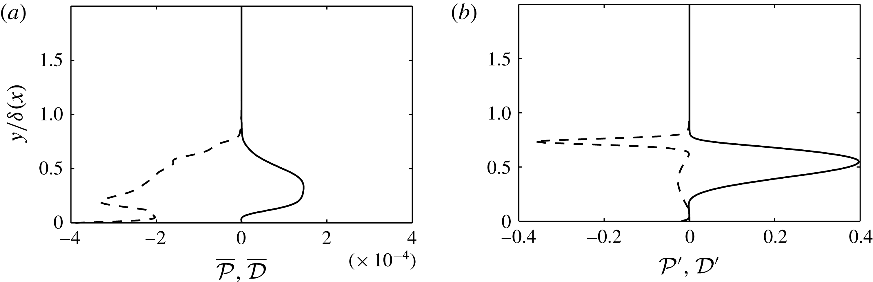
Results for the averaged production and dissipation of the fluctuation kinetic energy are provided in figure 12(a) and show that both quantities peak in the lower portion of the boundary layer and in the case of the dissipation at the wall. In contrast, the instantaneous dissipation profile has a localized sharp peak situated close to the edge of the boundary layer which exceeds the maximum of the average by three orders of magnitude. The magnitude of the instantaneous production surpasses the mean by a comparable ratio, although the shift away from the wall is less pronounced.
Profiles of terms of the fluctuation kinetic energy budget at the centre of the hairpin,
 $x=2.66$
,
 $z=0.15$
and
 $t=t_{0}+1.03$
. Production (solid) and dissipation (dashed). (a) Temporal and spanwise mean. (b) Instantaneous.

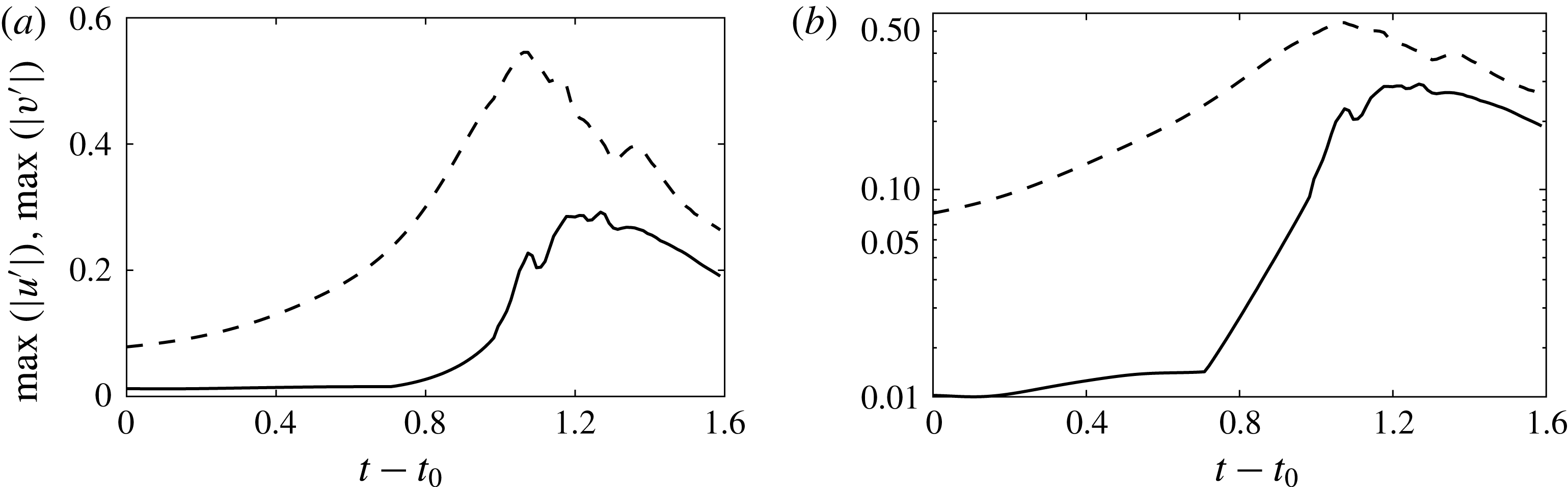
Peak normal (solid) and streamwise (dashed) velocity fluctuations during hairpin formation as a function of time. (a) Linear scaling. (b) Logarithmic scaling.

The temporal evolution of the peak streamwise and normal fluctuations generated by the transitional hairpin process is presented in figure 13(a). At
 $t=t_{0}$
, i.e. before the hairpin has formed,
 $u^{\prime }$
already has an appreciable amplitude, while
 $v^{\prime }$
is of the order of 1 %. At approximately
 $t_{0}+0.74$
, the amplitude of the
 $u^{\prime }$
fluctuation has increased to 0.25, and
 $v^{\prime }$
begins to amplify rapidly until it reaches a maximum of approximately 28 % of the free-stream velocity. Insight into the nature of the growth mechanism is gained by repeating the plot using a logarithmic scaling for the ordinate; see figure 13(b). The strong growth of
 $v^{\prime }$
between
 $t_{0}+0.72$
and circa
 $t_{0}+1.00$
is represented by a straight line, suggesting that the initial stage of the hairpin process that generates the extremely high fluctuation levels is driven by an exponential instability. It is worth clarifying that the exponential instability also influences the streamwise velocity fluctuations. However, due to the already high level of
 $u^{\prime }$
at the onset of the exponential instability, this effect is of subordinate importance. We further note that the exponential growth takes place after the initial growth of the Tollmien–Schlichting wave and the oblique mode, as studied, for instance, in the Floquet analyses of Herbert (Reference Herbert1988), has saturated. Considering these two instabilities as primary and secondary mechanisms, the hairpin mechanisms can be counted as the third exponential instability of the transitional boundary layer.
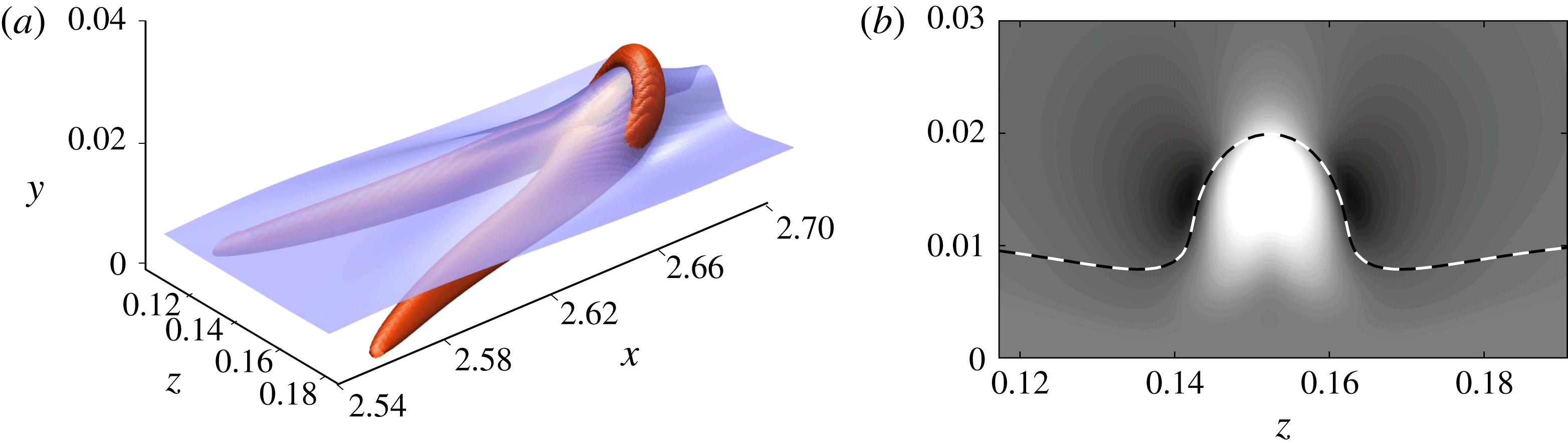
Further evidence for a connection between the growth mechanism at the core of the hairpin process and an exponential instability is gained from an evaluation of the instantaneous critical layer. The latter denotes the set of locations where the streamwise velocity instantaneously matches the propagation speed of the patches of high-intensity fluctuations at the centre of the hairpin. Linear theory suggests a concentration of the eigensolutions to the inviscid stability equations near the critical layer (Tollmien Reference Tollmien1929). For the specific case of the transitional hairpin, figure 14(a) presents the critical layer at
 $t=t_{0}+1.03$
, and demonstrates the spatial alignment with the flow structure. A cut plane through the tip of the hairpin at the same time instant is presented in figure 14(b). In line with observations of inviscid streak instabilities in bypass transition (e.g. Andersson et al.
Reference Andersson, Brandt, Bottaro and Henningson2001; Hack & Zaki Reference Hack and Zaki2014b
, Reference Hack and Zaki2016), the patches of positive and negative
 $v^{\prime }$
are centred around the critical layer. The present results thus extend the conclusions in the resolvent analysis by Sharma & McKeon (Reference Sharma and McKeon2013), who noted the alignment of their very-large-scale motions with the critical layer. While that observation was founded on the turbulent mean profile, the present case concerns an instantaneous observation.
4.2 Linear stability analysis
A conclusive characterization of the role of exponential growth mechanisms calls for an analysis of the hairpin process by means of linear stability theory. Ahead of the presentation of results, the methodology is briefly outlined in the following. As reported in § 2, the direct simulations were conducted with a code solving the compressible Navier–Stokes equations at a Mach number of
 $Ma=0.2$
. While compressibility effects are virtually absent in this setting, we maintain consistency with the nonlinear simulations by formulating the stability problem in terms of the compressible Navier–Stokes equations in conserved variables,
 $$\begin{eqnarray}\displaystyle & \displaystyle {\displaystyle \frac{\unicode[STIX]{x2202}\unicode[STIX]{x1D70C}}{\unicode[STIX]{x2202}t}}+{\displaystyle \frac{\unicode[STIX]{x2202}\unicode[STIX]{x1D70C}u_{j}}{\unicode[STIX]{x2202}x_{j}}}=0, & \displaystyle\end{eqnarray}$$
 $$\begin{eqnarray}\displaystyle & \displaystyle {\displaystyle \frac{\unicode[STIX]{x2202}m_{i}}{\unicode[STIX]{x2202}t}}+{\displaystyle \frac{\unicode[STIX]{x2202}\unicode[STIX]{x1D70C}u_{i}u_{j}}{\unicode[STIX]{x2202}x_{j}}}=-{\displaystyle \frac{\unicode[STIX]{x2202}p}{\unicode[STIX]{x2202}x_{i}}}+{\displaystyle \frac{\unicode[STIX]{x2202}}{\unicode[STIX]{x2202}x_{j}}}{\displaystyle \frac{\unicode[STIX]{x1D707}}{Re}}\left({\displaystyle \frac{\unicode[STIX]{x2202}u_{i}}{\unicode[STIX]{x2202}x_{j}}}+{\displaystyle \frac{\unicode[STIX]{x2202}u_{j}}{\unicode[STIX]{x2202}x_{i}}}-{\displaystyle \frac{2}{3}}{\displaystyle \frac{\unicode[STIX]{x2202}u_{k}}{\unicode[STIX]{x2202}x_{k}}}\unicode[STIX]{x1D6FF}_{ij}\right), & \displaystyle\end{eqnarray}$$
 $$\begin{eqnarray}\displaystyle & \displaystyle {\displaystyle \frac{\unicode[STIX]{x2202}e}{\unicode[STIX]{x2202}t}}+{\displaystyle \frac{\unicode[STIX]{x2202}}{\unicode[STIX]{x2202}x_{j}}}\left[pu_{j}{\displaystyle \frac{\unicode[STIX]{x1D6FE}}{\unicode[STIX]{x1D6FE}-1}}+{\displaystyle \frac{1}{2}}\unicode[STIX]{x1D70C}u_{k}u_{k}u_{j}\right]={\displaystyle \frac{\unicode[STIX]{x2202}}{\unicode[STIX]{x2202}x_{j}}}{\displaystyle \frac{\unicode[STIX]{x1D707}}{Re\;Pr}}{\displaystyle \frac{\unicode[STIX]{x2202}T}{\unicode[STIX]{x2202}x_{j}}} & \displaystyle \nonumber\\ \displaystyle & \displaystyle +\,{\displaystyle \frac{\unicode[STIX]{x2202}}{\unicode[STIX]{x2202}x_{j}}}{\displaystyle \frac{\unicode[STIX]{x1D707}}{Re}}\left(u_{k}\left({\displaystyle \frac{\unicode[STIX]{x2202}u_{k}}{\unicode[STIX]{x2202}x_{j}}}+{\displaystyle \frac{\unicode[STIX]{x2202}u_{j}}{\unicode[STIX]{x2202}x_{k}}}-{\displaystyle \frac{2}{3}}{\displaystyle \frac{\unicode[STIX]{x2202}u_{l}}{\unicode[STIX]{x2202}x_{l}}}\unicode[STIX]{x1D6FF}_{jk}\right)\right), & \displaystyle\end{eqnarray}$$
with
 $m_{i}=\unicode[STIX]{x1D70C}u_{i}$
. Ideal-gas behaviour is assumed, so that
 $$\begin{eqnarray}\unicode[STIX]{x1D70C}T=\frac{p\unicode[STIX]{x1D6FE}}{\unicode[STIX]{x1D6FE}-1},\end{eqnarray}$$
where
 $\unicode[STIX]{x1D6FE}$
is the ratio of the specific heats. Linearization of the equations around a time-invariant base state
 $\bar{\boldsymbol{q}}(x,y,z)=(\bar{\unicode[STIX]{x1D70C}},\bar{m}_{1},\bar{m}_{2},\bar{m}_{3},\bar{e})^{\text{T}}$
yields
 $$\begin{eqnarray}\frac{\unicode[STIX]{x2202}\boldsymbol{q}^{\prime }}{\unicode[STIX]{x2202}t}+\frac{\unicode[STIX]{x2202}\boldsymbol{F}_{i}^{\prime }}{\unicode[STIX]{x2202}x_{i}}=0\end{eqnarray}$$
and
 $$\begin{eqnarray}\unicode[STIX]{x1D70C}^{\prime }\bar{T}+\bar{\unicode[STIX]{x1D70C}}T^{\prime }=\frac{p^{\prime }\unicode[STIX]{x1D6FE}}{\unicode[STIX]{x1D6FE}-1},\end{eqnarray}$$
with
(a) Isolated hairpin at
 $t=t_{0}+1.03$
with critical layer (blue). (b) Cross-section at
 $x=2.67$
with contours of
 $v^{\prime }$
from
 $-0.1$
(black) to 0.1 (white). The dashed line marks the instantaneous critical layer.

 $$\begin{eqnarray}\boldsymbol{q}^{\prime }\equiv \left(\begin{array}{@{}c@{}}\unicode[STIX]{x1D70C}^{\prime }\\ m_{1}^{\prime }\\ m_{2}^{\prime }\\ m_{3}^{\prime }\\ e^{\prime }\end{array}\right),\quad \boldsymbol{F}_{i}^{\prime }\equiv \left(\begin{array}{@{}c@{}}\bar{\unicode[STIX]{x1D70C}}u_{i}^{\prime }+\unicode[STIX]{x1D70C}^{\prime }\bar{u_{i}}\\ \bar{\unicode[STIX]{x1D70C}}\bar{u_{1}}u_{i}^{\prime }+\bar{\unicode[STIX]{x1D70C}}u_{1}^{\prime }\bar{u_{i}}+\unicode[STIX]{x1D70C}^{\prime }\bar{u_{1}}\bar{u_{i}}+p^{\prime }\unicode[STIX]{x1D6FF}_{i1}-\unicode[STIX]{x1D70E}_{i1}^{\prime }\\ \bar{\unicode[STIX]{x1D70C}}\bar{u_{2}}u_{i}^{\prime }+\bar{\unicode[STIX]{x1D70C}}u_{2}^{\prime }\bar{u_{i}}+\unicode[STIX]{x1D70C}^{\prime }\bar{u_{2}}\bar{u_{i}}+p^{\prime }\unicode[STIX]{x1D6FF}_{i2}-\unicode[STIX]{x1D70E}_{i2}^{\prime }\\ \bar{\unicode[STIX]{x1D70C}}\bar{u_{3}}u_{i}^{\prime }+\bar{\unicode[STIX]{x1D70C}}u_{3}^{\prime }\bar{u_{i}}+\unicode[STIX]{x1D70C}^{\prime }\bar{u_{3}}\bar{u_{i}}+p^{\prime }\unicode[STIX]{x1D6FF}_{i3}-\unicode[STIX]{x1D70E}_{i3}^{\prime }\\ \unicode[STIX]{x1D701}_{i}^{\prime }+\unicode[STIX]{x1D705}_{i}^{\prime }+\unicode[STIX]{x1D709}_{i}^{\prime }\end{array}\right)\end{eqnarray}$$
and
 $$\begin{eqnarray}\displaystyle & \displaystyle m_{i}^{\prime }\equiv \bar{\unicode[STIX]{x1D70C}}u_{i}^{\prime }+\unicode[STIX]{x1D70C}^{\prime }\bar{u}_{i}, & \displaystyle\end{eqnarray}$$
 $$\begin{eqnarray}\displaystyle & \displaystyle e^{\prime }\equiv p^{\prime }/\left(\unicode[STIX]{x1D6FE}-1\right)+\bar{\unicode[STIX]{x1D70C}}\bar{u}_{k}u_{k}^{\prime }+\unicode[STIX]{x1D70C}^{\prime }\bar{u}_{k}\bar{u}_{k}/2, & \displaystyle\end{eqnarray}$$
 $$\begin{eqnarray}\displaystyle & \displaystyle \unicode[STIX]{x1D70E}_{ij}^{\prime }\equiv \frac{\unicode[STIX]{x1D707}}{Re}\left(\frac{\unicode[STIX]{x2202}u_{i}^{\prime }}{\unicode[STIX]{x2202}x_{j}}+\frac{\unicode[STIX]{x2202}u_{j}^{\prime }}{\unicode[STIX]{x2202}x_{i}}-\frac{2}{3}\frac{\unicode[STIX]{x2202}u_{k}^{\prime }}{\unicode[STIX]{x2202}x_{k}}\unicode[STIX]{x1D6FF}_{ij}\right)\!, & \displaystyle\end{eqnarray}$$
 $$\begin{eqnarray}\displaystyle & \displaystyle \unicode[STIX]{x1D701}_{i}^{\prime }\equiv \left(\bar{p}u_{i}^{\prime }+p^{\prime }\bar{u_{i}}\right)\frac{\unicode[STIX]{x1D6FE}}{\unicode[STIX]{x1D6FE}-1}+\frac{1}{2}\left(\bar{\unicode[STIX]{x1D70C}}\bar{u}_{k}\bar{u}_{k}u_{i}^{\prime }+2\bar{\unicode[STIX]{x1D70C}}\bar{u}_{k}u_{k}^{\prime }\bar{u}_{i}+\unicode[STIX]{x1D70C}^{\prime }\bar{u}_{k}\bar{u}_{k}\bar{u}_{i}\right)\!, & \displaystyle\end{eqnarray}$$
 $$\begin{eqnarray}\displaystyle & \displaystyle \unicode[STIX]{x1D705}_{i}^{\prime }\equiv -\frac{\unicode[STIX]{x1D707}}{Re\;Pr}\frac{\unicode[STIX]{x2202}T^{\prime }}{\unicode[STIX]{x2202}x_{i}}, & \displaystyle\end{eqnarray}$$
 $$\begin{eqnarray}\displaystyle & \displaystyle \unicode[STIX]{x1D709}_{i}^{\prime }\equiv \frac{\unicode[STIX]{x1D707}}{Re}\left(\bar{u}_{j}\frac{\unicode[STIX]{x2202}u_{j}^{\prime }}{\unicode[STIX]{x2202}x_{i}}+u_{j}^{\prime }\frac{\unicode[STIX]{x2202}\bar{u}_{j}}{\unicode[STIX]{x2202}x_{i}}+\bar{u}_{j}\frac{\unicode[STIX]{x2202}u_{i}^{\prime }}{\unicode[STIX]{x2202}x_{j}}+u_{j}^{\prime }\frac{\unicode[STIX]{x2202}\bar{u}_{i}}{\unicode[STIX]{x2202}x_{j}}-\frac{2}{3}\left(\bar{u}_{j}\frac{\unicode[STIX]{x2202}u_{l}^{\prime }}{\unicode[STIX]{x2202}x_{l}}\unicode[STIX]{x1D6FF}_{ij}+u_{j}^{\prime }\frac{\unicode[STIX]{x2202}\bar{u}_{l}}{\unicode[STIX]{x2202}x_{l}}\unicode[STIX]{x1D6FF}_{ij}\right)\right) & \displaystyle\end{eqnarray}$$
where
 $\unicode[STIX]{x1D6FF}_{ij}$
is the Kronecker delta. The rapid amplification of normal perturbations observed in figure 13 suggests that the underlying instability operates on an appreciably shorter time scale than the variation of the base flow. This separation of scales justifies the above assumption of a frozen base flow and leads to normal-mode behaviour in time, so that
 $$\begin{eqnarray}\boldsymbol{q}^{\prime }(t)=\hat{\boldsymbol{q}}\exp (-\text{i}\unicode[STIX]{x1D70E}t).\end{eqnarray}$$
Introduction into the governing equations (4.8) gives rise to an eigenvalue problem of the form
 $$\begin{eqnarray}-\text{i}\unicode[STIX]{x1D70E}\hat{\boldsymbol{q}}=\unicode[STIX]{x1D647}\hat{\boldsymbol{q}}.\end{eqnarray}$$
The base flow of the analysis is obtained by extracting a three-dimensional region from the direct simulations at the beginning of the interval of strong exponential growth,
 $t_{0}+0.72$
, coinciding with the sharp change in the slope of
 $\max (|v^{\prime }|)$
in figure 13. At this instant, the streamwise velocity perturbation has already reached appreciable amplitude, while normal and spanwise fluctuations are of the order of 1 % of the free-stream velocity. Homogeneous boundary conditions are applied in all spatial dimensions,
 $\hat{\boldsymbol{q}}|_{\unicode[STIX]{x2202}\unicode[STIX]{x1D6FA}}\equiv 0$
. Spurious reflections from the boundaries are dampened through a sponge layer. Consistent with the direct simulations, the spatial discretization is based on fourth-order finite differences and uses 128 grid points in all dimensions. The resulting eigenvalue problem is of dimension
 $128\times 128\times 128\times 5\approx 1.05\times 10^{7}$
and is solved using a parallel implementation of the implicitly restarted Arnoldi method (Sorensen Reference Sorensen1992; Maschhoff & Sorensen Reference Maschhoff, Sorensen, Waśniewski, Dongarra, M. K. and Olesen1996).
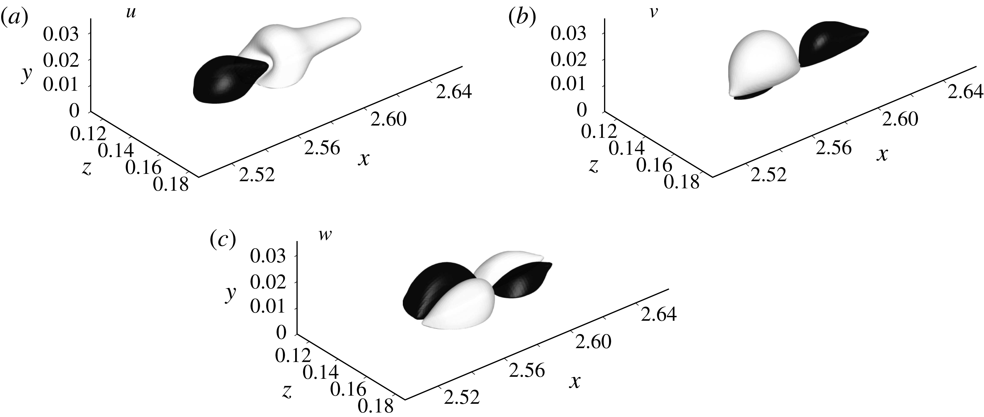
Isosurfaces of the primary eigenfunction computed at
 $t=t_{0}+0.74$
. Streamwise, normal and spanwise components: positive (white) and negative (black).

The velocity components of the first eigenfunction computed in the present stability analysis are visualized in figure 15. The eigenfunction is exponentially unstable with a growth rate of
 $\unicode[STIX]{x1D70E}_{i}=10.62$
, which moderately exceeds the amplification observed in the DNS. The phase speed of the mode is
 $c_{r}=0.40$
. The eigenfunction is spatially localized at the centre of the computational domain, with its streamwise extent limited to a single (fundamental) wavelength. The complex structure of the eigenfunction nonetheless suggests the presence of higher harmonics in all spatial dimensions.
In the context of Görtler flow, Swearingen & Blackwelder (Reference Swearingen and Blackwelder1987) introduced a classification of secondary instabilities into sinuous and varicose types. The sinuous instability is characterized by a spanwise antisymmetric arrangement of the streamwise and normal components of the eigenfunction and a spanwise symmetric arrangement of the spanwise component. In the varicose instability, this pattern is inverted such that the streamwise and normal components are spanwise symmetric and the spanwise component is antisymmetric. Application of this categorization to the present results identifies the instability at the core of the hairpin process as varicose. This outcome is consistent with earlier observations in the context of bypass transition to turbulence, where a connection between varicose instabilities and the formation of hairpins was demonstrated both experimentally and computationally (Asai, Minagawa & Nishioka Reference Asai, Minagawa and Nishioka2002; Hack & Zaki Reference Hack and Zaki2014b ).
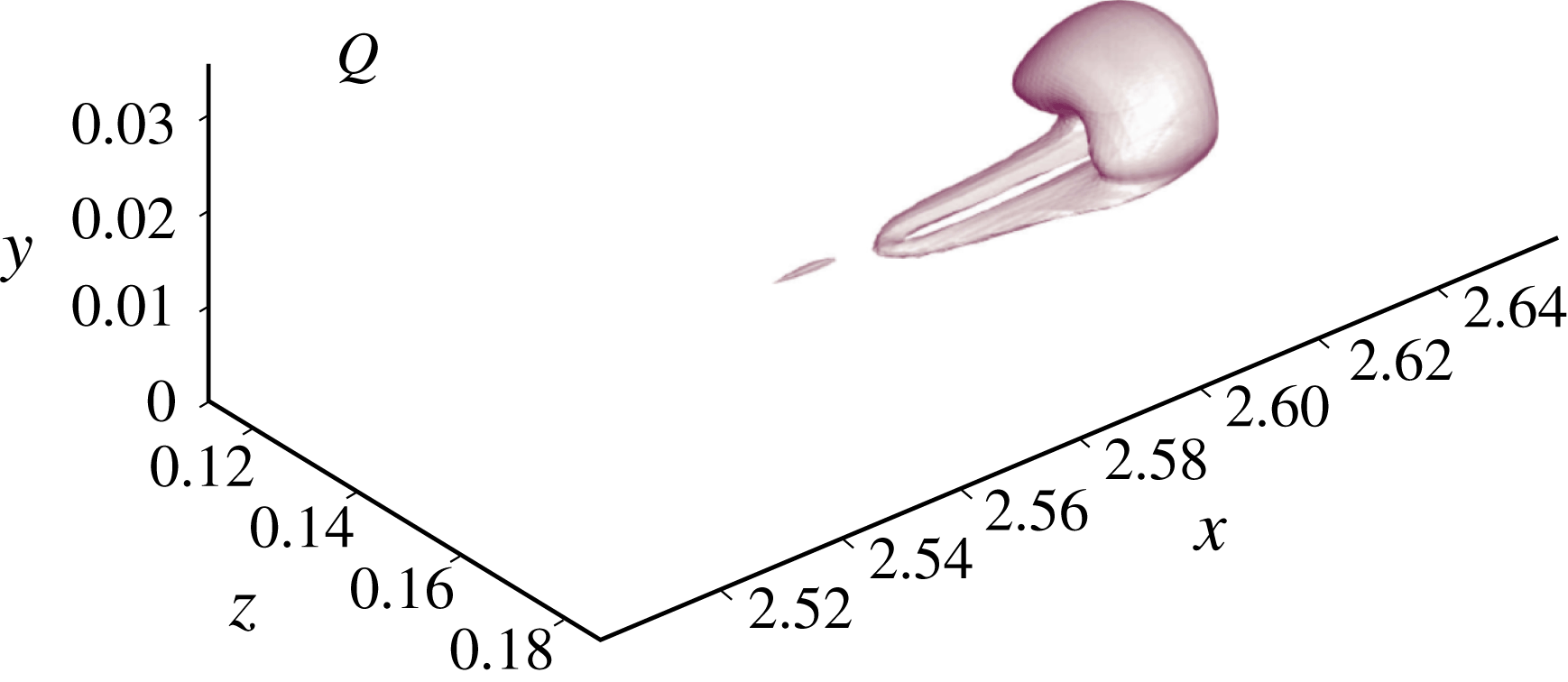
The linear analysis provides graphic evidence for the connection between the linear instability mechanism and the formation of the arc-shaped structures that popularly define the hairpin process. Application of the
 $Q$
criterion to the most unstable eigenfunction generates a field whose spatial structure resembles the hairpin observed in the nonlinear direct simulations; see figure 16. A prominent tip is connected to two thin legs of relatively short extent and narrow spacing. While its proportions differ from the DNS visualizations, the structure contains the characteristic elements of a hairpin and would in fact be identified by the topological classification algorithm introduced in this work. In providing a rudimentary representation of the topological features of the nonlinear structure, the ‘linear hairpin’ is representative of the broader context. While our results strongly suggest that the transitional hairpin process is at its core related to a linear instability mechanism, it is appreciably modulated and reshaped by nonlinear effects.
We note that the present base flow of a boundary layer distorted by an isolated region of low-speed fluid, as visualized, for instance, in the first frame of figure 7, is represented by a multitude of Fourier modes in the streamwise dimension. As a consequence, the results obtained in the linear analysis are not amenable to a direct transformation between inertial frames moving at different velocities. In the interest of the comparability of the results, we have thus elected to present results from a stability analysis conducted in a stationary reference frame. Analyses in a frame moving with the phase speed of the patch of negative streamwise velocity fluctuations resulted in effectively identical eigensolutions.
Isosurface of the
 $Q$
criterion computed for the primary eigenfunction at
 $t=t_{0}+0.74$
.

By relating the transitional hairpins to a robust exponential instability mechanism, linear theory can thus be concluded to provide a well-founded explanation for their prevalence under various conditions which transcends kinematic models. Since the undistorted mean of the zero-pressure-gradient boundary layer is stable to inviscid instabilities, the amplification can be attributed to a secondary instability due to an earlier perturbation of the flow field. In particular, the structure of the hairpin as commonly visualized through vortex identification criteria can be seen as a symptom of the instability which requires a pre-existing perturbation to amplify.
4.3 Packet formation and breakdown to turbulence
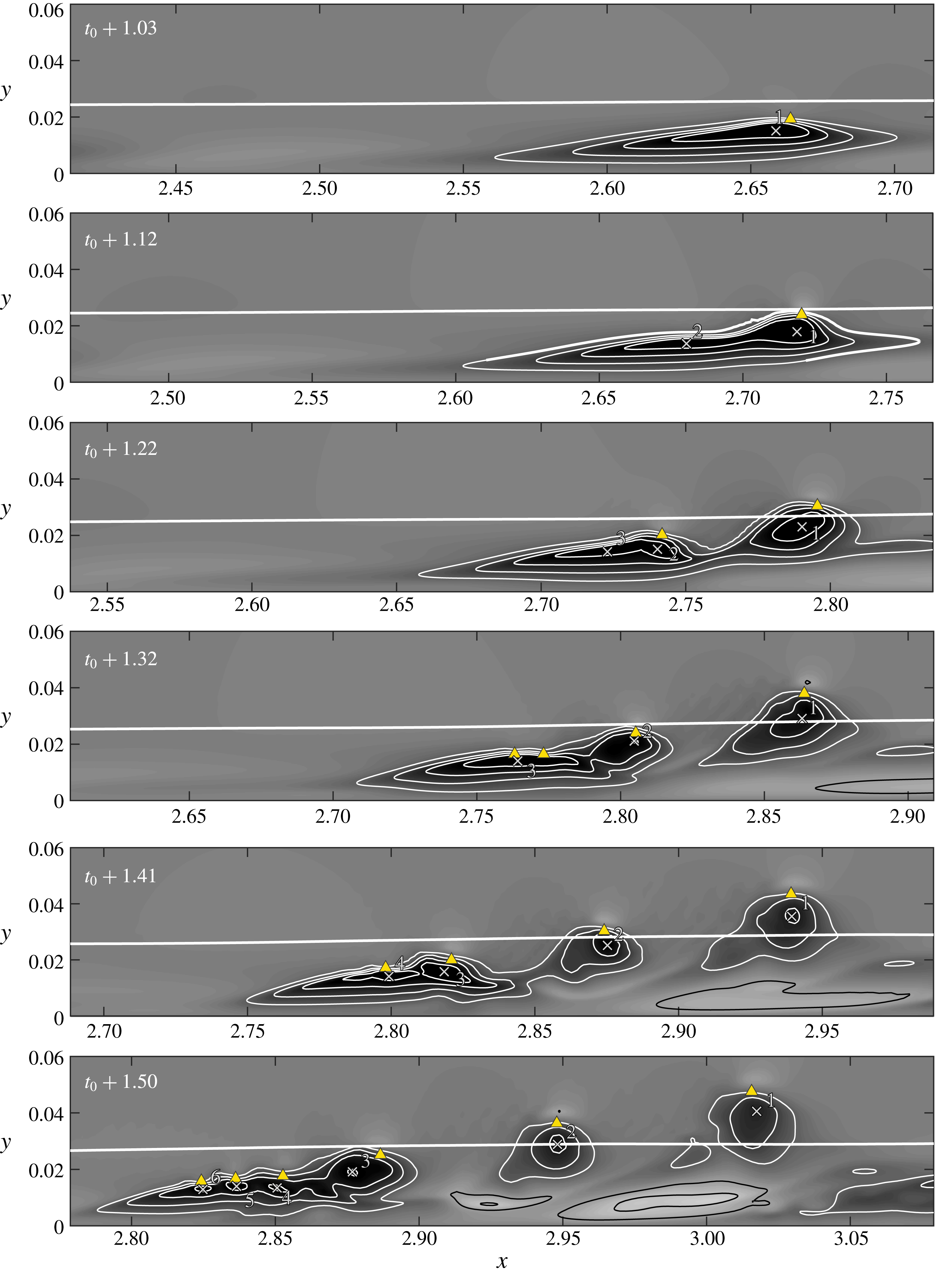
Studies of turbulent wall-bounded flows have reported the occurrence of groups of hairpin vortices that propagate at comparable speed. Among others, Zhou et al. (Reference Zhou, Adrian, Balachandar and Kendall1999) and Adrian et al. (Reference Adrian, Meinhart and Tomkins2000) refer to these groups as packets of hairpins. A similar behaviour is observed in the late-stage transitional flow as visualized in the time series of figures 7 and 8. In the fourth and fifth frames, a second hairpin forms downstream of the first, followed by a series of smaller arc-shaped structures in the
 $Q$
criterion.
Hairpin packet formation in the transitional boundary layer. Time series of side view with contours of the streamwise fluctuation,
 $u^{\prime }$
. Crosses and numbers indicate local minima of
 $u^{\prime }$
, triangles indicate the heads of hairpins. The continuous white line marks the local boundary layer thickness.

Insight into the dynamics of the generation of a hairpin packet in late-stage transitional flow is provided by the time series presented in figure 17. Planes at
 $z=0.152$
, coinciding with the spanwise centre of the hairpin vortices, show contours of the streamwise velocity fluctuation. Crosses mark the locations of local minima of
 $u^{\prime }$
, and numbers identify the same extremum across frames. The first frame shows the flow field at
 $t=t_{0}+1.03$
, the time at which the streamwise fluctuations reach their highest level. At this instant, the patch of negative
 $u^{\prime }$
has a single extremum of highest intensity which coincides with the head of the hairpin structure marked by the triangle. As the flow evolves, a second local extremum forms, and, at time
 $t=t_{0}+1.22$
, the patch has started to split into two distinct regions. Comparison with figure 7 shows that this process coincides with the separation of the primary hairpin at the upstream edge of the region of low-speed fluid and the formation of a secondary hairpin in the remaining patch. The low-velocity fluid associated with the primary hairpin lifts away from the wall and loses intensity. At
 $t=t_{0}+1.41$
, the hairpin associated with local minimum 2 also begins to separate as further local extrema are generated. While the remaining patch stays close to the wall, the separated extrema rise towards the edge of the boundary layer and travel at faster speed. The continuous separation of smaller regions from the large patch of negative
 $u^{\prime }$
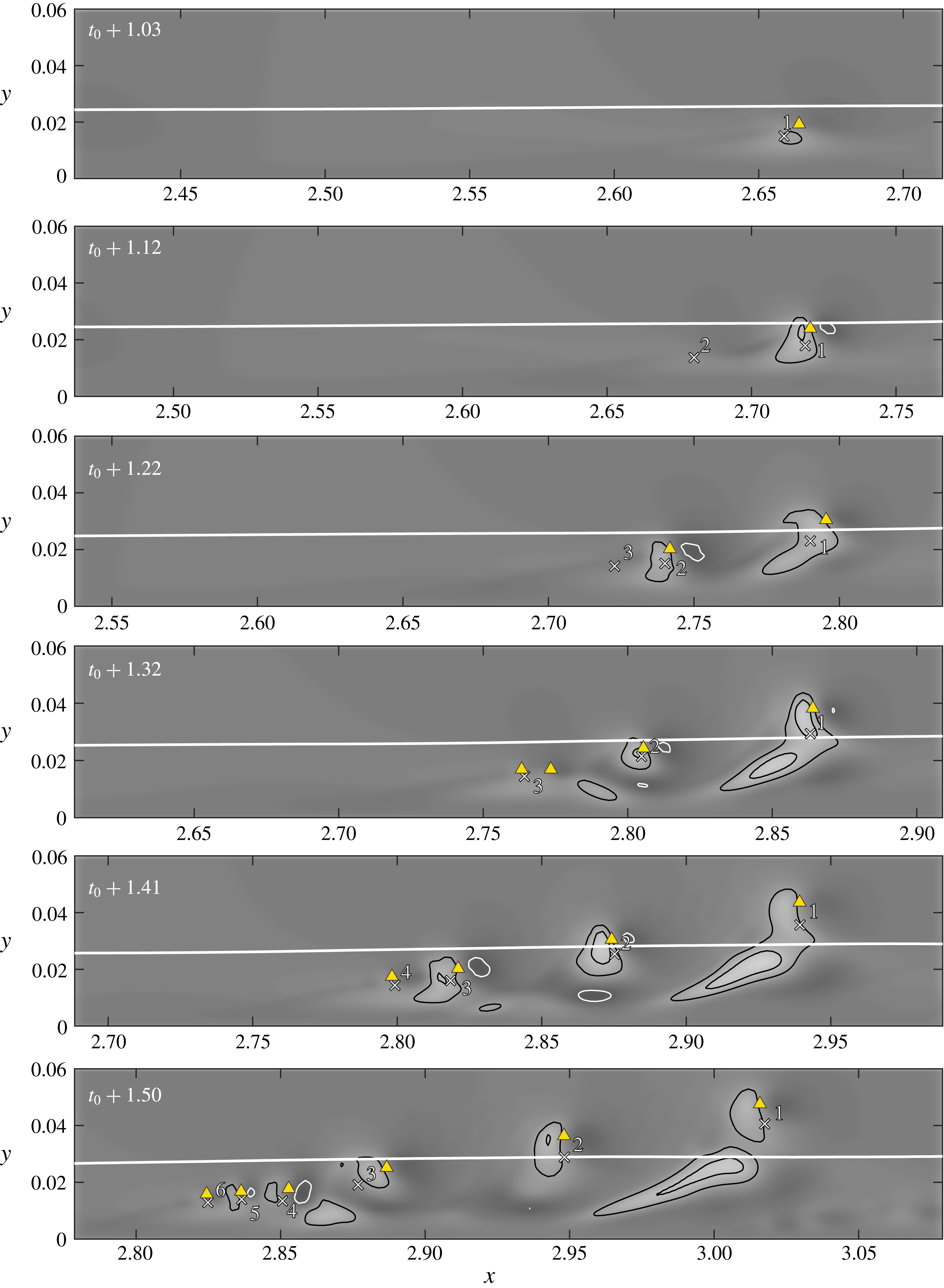
appears as a self-similar process which continues until the patch eventually breaks up. A time series of the normal fluctuations is presented in figure 18, indicating that the locations of the positive normal fluctuations spatially coincide with the patches of negative streamwise fluctuations observed in figure 17. We also note that the original hairpin does not participate in the breakdown to turbulence which originates from the tail end of the region of low momentum where the shortest wavelengths are generated.
Hairpin packet formation in the transitional boundary layer. Time series of side view with contours of the normal fluctuation,
 $v^{\prime }$
. Crosses and numbers indicate local minima of
 $u^{\prime }$
, triangles indicate the heads of hairpins. The continuous white line marks the local boundary layer thickness.

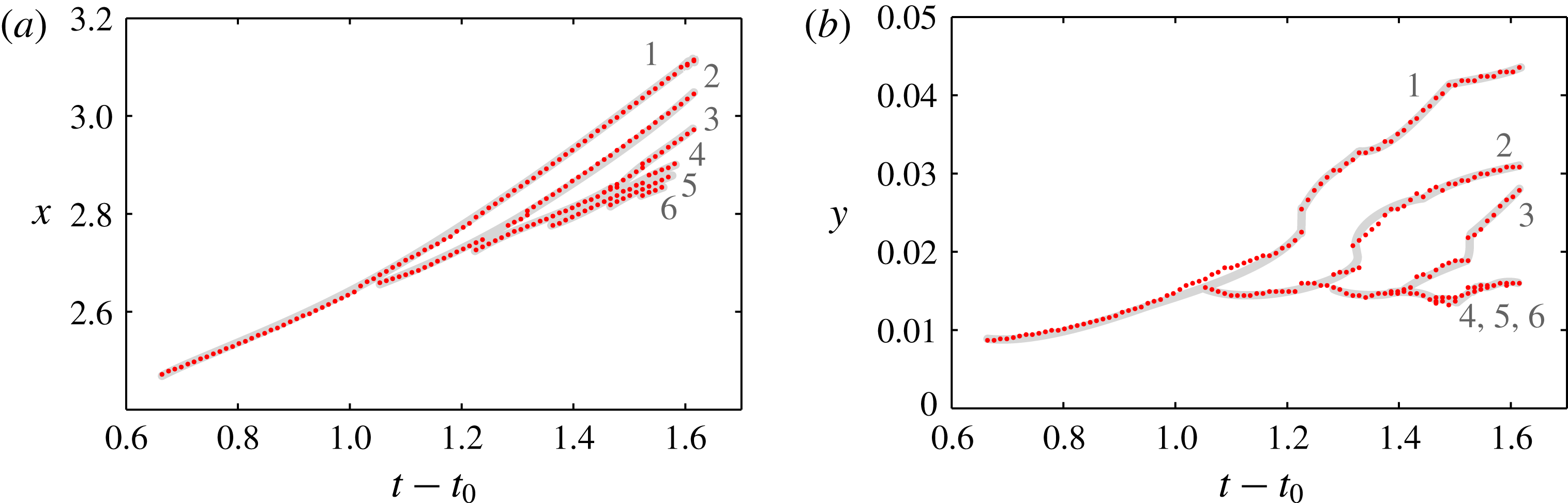
The streamwise positions of the local minima of
 $u^{\prime }$
as a function of time are shown in figure 19(a). Initially, the single region of low-speed fluid travels at a nearly constant speed of
 $c\approx 0.52$
. At
 $t\approx 1.05$
, the first local maximum separates and accelerates to a higher speed of
 $c\approx 0.77$
, leaving behind the slower remainder of the patch, which at
 $t\approx 1.25$
again splits. The self-similar nature of the breakup of the region of negative
 $u^{\prime }$
is reflected in the identical slopes of each of the separated extrema. The normal positions of the local minima of the streamwise fluctuations are presented in figure 19(b). While the separated minima rapidly move away from the wall, the remaining patch of low-speed fluid never exceeds a wall distance of
 $y\approx 0.016$
.
Trajectories of the local minima of the streamwise fluctuation during the late stages of natural transition. (a) Streamwise position as a function of time. (b) Normal position as a function of time.

It was shown in § 4.2 that the formation of the first hairpin can be connected to the growth of an inviscid secondary instability of varicose type caused by a distortion of the boundary layer through a localized region of low-speed fluid. A second instability analysis is conducted at
 $t=t_{0}+1.03$
to examine whether the splitting of this region and the associated formation of a packet of hairpins can also be related to linear stability theory. The streamwise component of the most unstable eigenfunction is presented in figure 20. The spanwise symmetric structure of the eigenfunction again suggests an instability of varicose type. In particular, it predicts an alternating pattern of negative and positive perturbations in the streamwise velocity component at a short streamwise wavelength of approximately 0.01, consistent with the breakup of the patch of low-speed fluid. The result thus suggests that while nonlinear effects can be expected to play an appreciable role, the splitting of the patch of low-speed fluid and the associated formation of a packet of hairpins can be related to linear theory.
Primary eigenfunction at
 $t=t_{0}+1.03$
. Isosurfaces of positive (white) and negative (black) streamwise component.

Before moving on to the turbulent flow regime, it is worth summarizing the insight gained from the analysis of the transitional hairpin process. The above results represent strong evidence for a connection between the formation of the coherent structure and an exponential instability mechanism. The instability is of varicose type and is triggered by a pre-existing predominantly streamwise distortion of the base flow which is an outcome of the earlier stages of the transition process. In terms of the causality of events, the results indicate that the hairpin structure is a symptom of this varicose instability mechanism rather than being the primary cause of the perturbation of the boundary layer. Finally, the results connect the formation of packets of hairpins to the same varicose instability mechanism.
5 Turbulent flow
As the flow progresses from the transitional regime towards a turbulent state, visualizations initially show an abundance of clearly recognizable hairpin structures (e.g. Wu & Moin Reference Wu and Moin2009; Sayadi et al. Reference Sayadi, Hamman and Moin2013). With growing Reynolds number, the structural topology of the flow becomes increasingly distorted by the broadening spectrum of turbulent length scales. As demonstrated in earlier studies, this distortion should, however, not be interpreted as an affirmation for the absence of the hairpin process which is recovered in a statistical sense (see, e.g., Dennis & Nickels Reference Dennis and Nickels2011a ,Reference Dennis and Nickels b ). Recent phenomenological evidence further suggests that individual hairpins continue to exist throughout the turbulent boundary layer at relatively high Reynolds numbers (Wu et al. Reference Wu, Moin, Wallace, Skarda, Lozano-Durán and Hickey2017). In the following, we seek to provide a time-resolved characterization of the turbulent hairpin and investigate whether the underlying flow physics agrees with the transitional hairpin process. A study of an individual hairpin isolated from turbulent flow at moderate Reynolds number is followed by statistical results gained from a large number of samples.
5.1 Turbulent hairpin
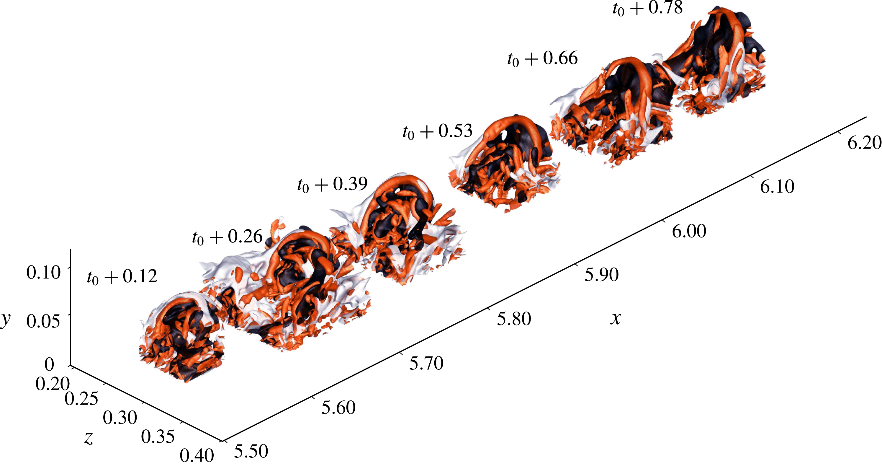
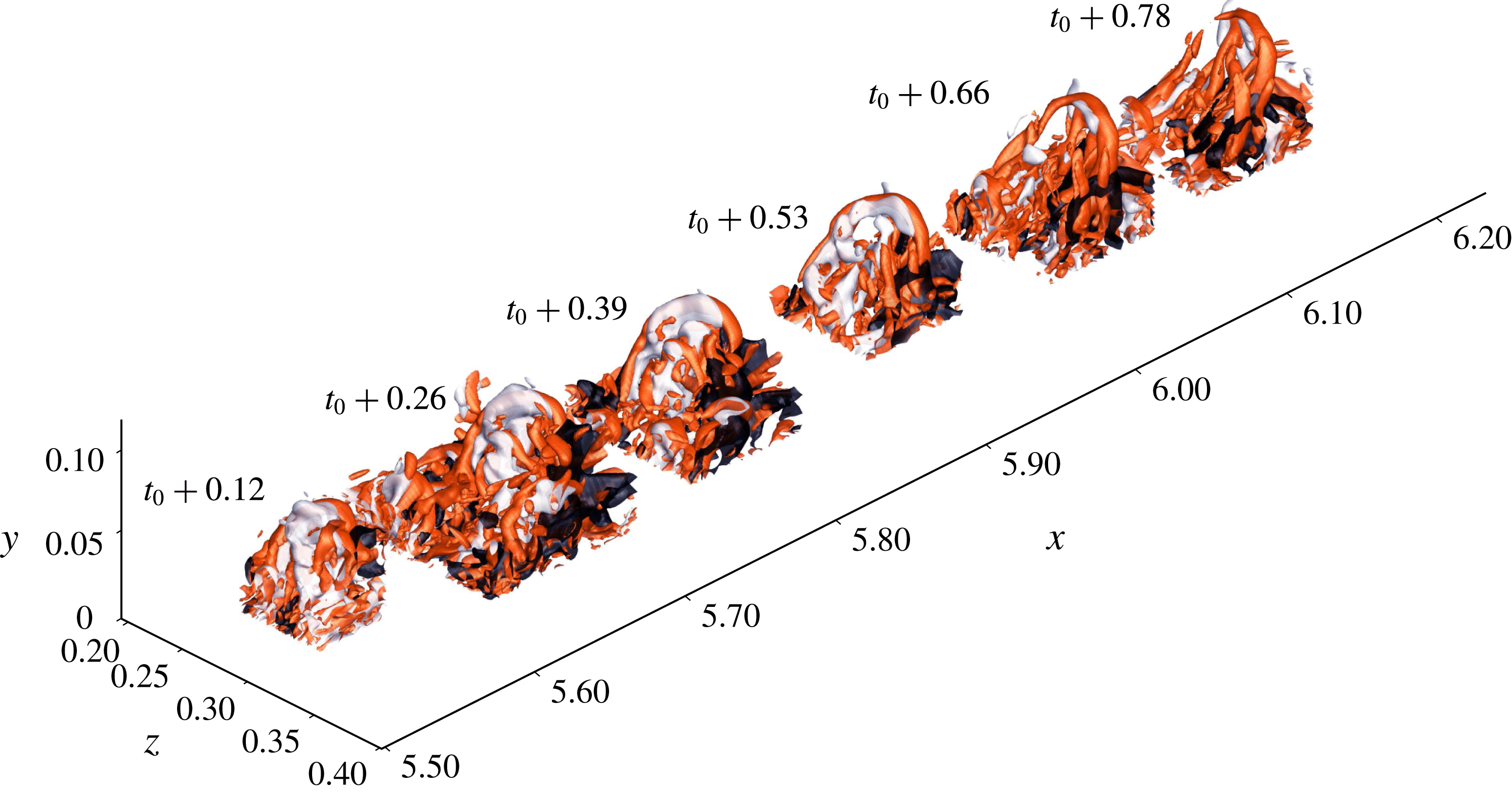
The evolution of an individual hairpin process identified in turbulent flow is considered. The hairpin is traced and isolated from the flow field by applying the identification scheme described in § 3. A series showing stages of the hairpin at varying times and locations as it travels downstream is presented in figures 21 and 22. In terms of the streamwise velocity fluctuations, the arch of the hairpin encloses a region of low-speed fluid at its centre while the fluid to the left and right is of higher velocity, thus representing positive fluctuations. These observations are largely consistent with the classical model of the hairpin that has been put forward in a wide body of literature, although it is worth pointing out that the streamwise extent of the region of low-speed fluid appears to be relatively limited in the present case.
Evolution of an individual hairpin in turbulent flow. Isosurfaces of negative (black) and positive (white) fluctuations of the streamwise velocity component with isosurfaces of the
 $Q$
criterion (red).

When considering the normal velocity component, the centre is host to a region of positive fluctuations, with negative fluctuations prevalent in the region outside of the arch. This outcome conforms with earlier reports of ejection events and even bursts of highly energetic momentum transport away from the wall coinciding with the hairpin process (e.g. Kim & Moin Reference Kim and Moin1986). In particular, the spatial arrangement of the patches of positive and negative fluctuations agrees with the transitional hairpin for both the streamwise and the normal components.
Evolution of an individual hairpin in turbulent flow. Isosurfaces of negative (black) and positive (white) fluctuations of the normal velocity component with isosurfaces of the
 $Q$
criterion (red).

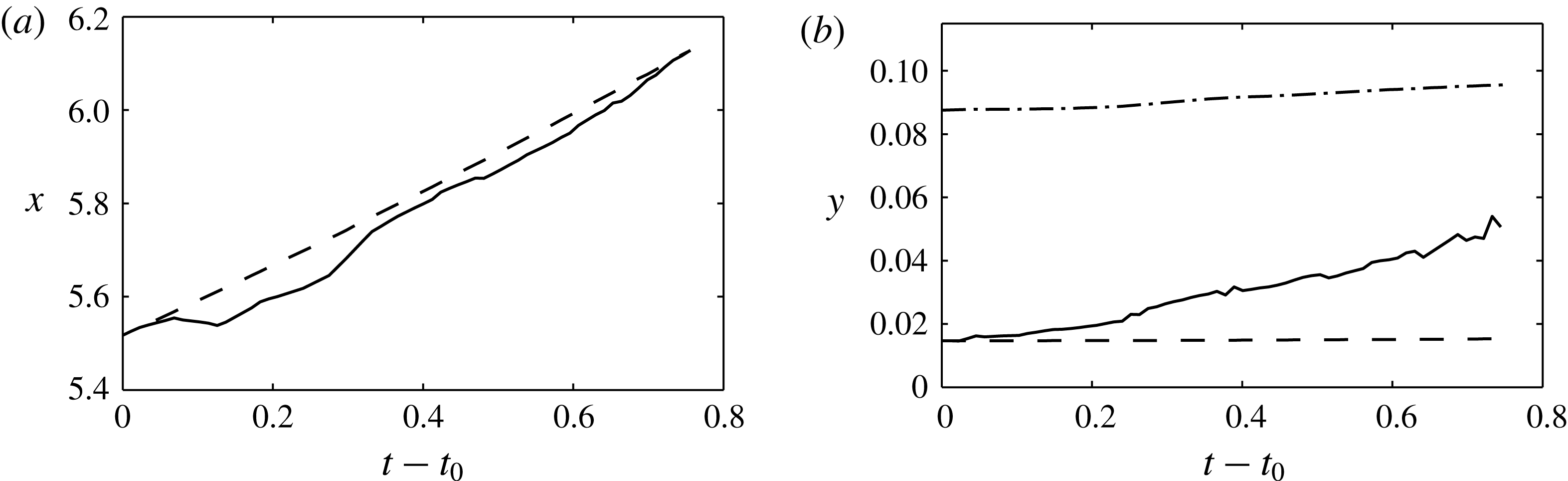
The trajectory of the hairpin in the boundary layer during its lifetime, measured as the position of the location of highest absolute streamwise fluctuation,
 $|u^{\prime }|$
, is presented in figure 23. The streamwise location follows an approximately linear trend, suggesting that the sampled hairpin travels at a nearly constant speed of
 $u_{c}\approx 0.75U_{\infty }$
. In an analogy to the transitional hairpin process, this speed matches that of the primary hairpin after its separation from the remaining patch of low-speed fluid, cf. figure 19(a). Also shown is the trajectory obtained by integrating the local mean velocity along the trajectory of the centre of the hairpin,
 $\overline{x}=\int \overline{u}\,\text{d}t$
. The coincidence of the end points of the two lines indicates that the streamwise movement of the hairpin closely follows a trajectory described by the mean flow. The normal position of the hairpin as a function of time is presented in figure 23(b). Also included are the normal mean flow trajectory, obtained by integrating the normal mean velocity component in time,
 $\overline{y}=\int \overline{v}\,\text{d}t$
, and the local boundary layer thickness. Comparison between the three trajectories shows that the normal movement of the hairpin clearly outpaces both the expansion of the boundary layer and the mean trajectory.
Trace of the turbulent hairpin. (a) Streamwise position as a function of time. Location of minimal
 $u^{\prime }$
(solid) and mean flow trajectory (dashed). (b) Normal position as a function of time. Location of minimal
 $u^{\prime }$
, mean flow trajectory (dashed) and local boundary layer thickness (dash-dotted).

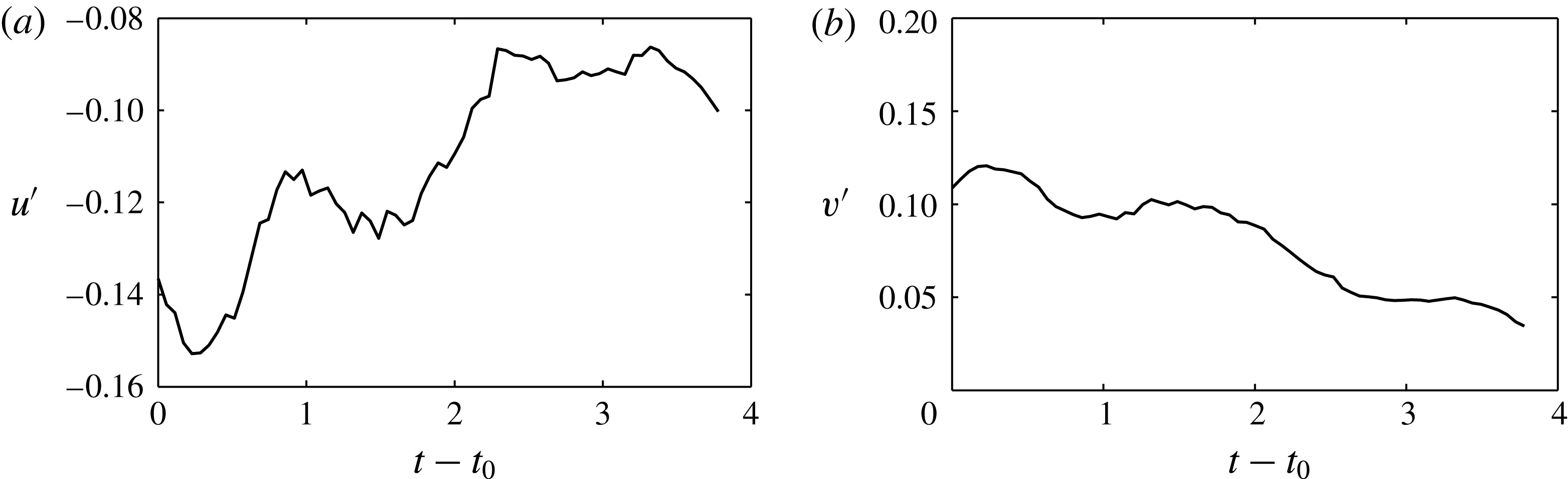
The most intense streamwise fluctuations within the volume occupied by the hairpin have a negative sign. Figure 24(a) presents the peak fluctuations as a function of time over the lifetime of the hairpin. By the time the hairpin is discernible in the flow, the streamwise velocity perturbation already has a relatively high amplitude of circa 14 % of the free-stream velocity. The amplitude initially grows further but relatively soon begins to decay and by the end of the lifetime of the hairpin has decreased to below 10 %. The peak normal fluctuations shown in figure 24(b) have a positive sign and qualitatively follow the trend of the streamwise component. Their peak amplitude coincides with the beginning of the life of the hairpin and is followed by a moderate but nearly monotonic decay. The quantitative trends observed are thus consistent with the transitional hairpin in the sense that, in that case, the streamwise fluctuations had also reached a relatively high amplitude at the time of the formation of the primary hairpin. A notable difference between the two classes of hairpins is in the level of the fluctuations, which are extremely high in the transitional case and exceed the peak amplitudes of the turbulent hairpin by a factor of three.
Evolution of the peak fluctuations in the turbulent hairpin. (a) Streamwise component. (b) Normal component.

Based on visual inspection, it appears unlikely that the filigree hairpin arch would be able to cause the comparatively large distortions of the streamwise velocity as predicted by some kinematic models. If, on the other hand, the hairpin is a symptom of a varicose secondary instability caused by an earlier perturbation in the base flow, one would expect to be able to identify this instability by means of linear analysis, analogous to the transitional case. A stability analysis is conducted at the first considered time instant,
 $t=t_{0}$
. The computational set-up is identical to the transitional case described in § 4.2 in terms of methodology and boundary conditions.
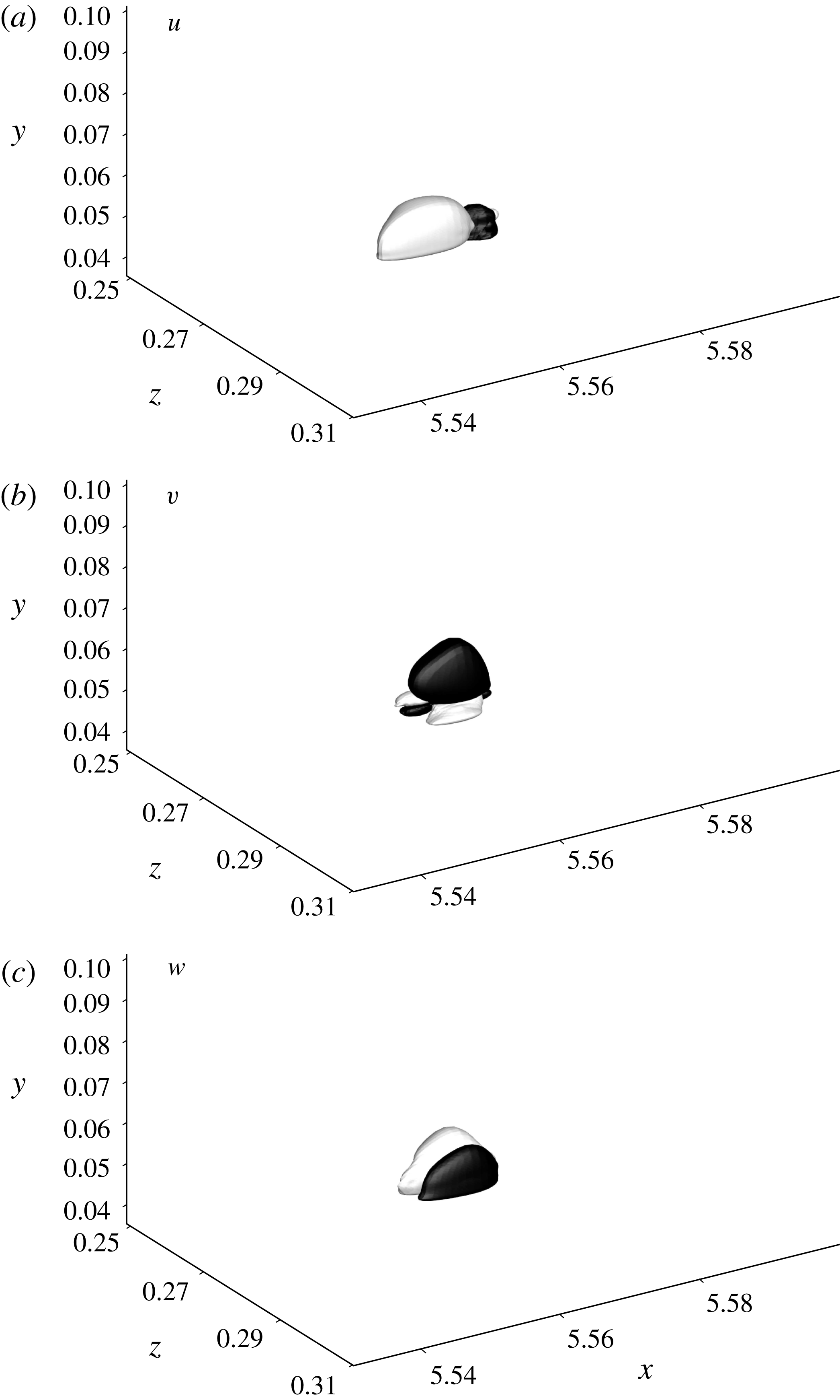
The most unstable eigenfunction computed in the stability analysis is presented in figure 25. In agreement with the transitional hairpin, the mode is again of varicose type and is characterized by transverse symmetric streamwise and normal components and a transverse antisymmetric spanwise component. The eigenfunction is spatially localized at the centre of the tip of the hairpin. Due to the complexity of the flow field, the turbulent hairpin cannot be expected to precisely follow the linear dynamics obtained in the analysis. However, the existence of a varicose instability that spatially coincides with the position of the hairpin can be seen as sound evidence for a connection to linear theory.
Primary eigenfunction of the turbulent hairpin process. Isosurfaces of negative (black) and positive (white) fluctuations. (a) Streamwise component, (b) normal component, (c) spanwise component.

5.2 Dynamic averaging
While the analysis of an individual turbulent hairpin in a natural setting and in the absence of artificial forcing conditions is insightful, it also raises questions about the universality of the results. The chaotic nature of turbulence innately implies that each manifestation of the hairpin process takes a unique form. We therefore seek statistical relevance by applying the structure identification algorithm to the full turbulent extent of the flow field and sampling all hairpins that occur during the length of the time series. For the purpose of processing the generated data, we introduce a time-resolved averaging methodology which normalizes the sampled structures with respect to their spatial extent but also with respect to their lifetime,
 $$\begin{eqnarray}\langle \boldsymbol{u}^{\prime }\rangle (\tilde{x},{\tilde{y}},\tilde{z},\unicode[STIX]{x1D70F})=\frac{1}{N}\mathop{\sum }_{n=1}^{N}\unicode[STIX]{x1D60E}_{5}(\boldsymbol{u}^{\prime },x,y,z,t)\boldsymbol{u}^{\prime }(x,y,z,t).\end{eqnarray}$$
Here, the operator
 $\unicode[STIX]{x1D60E}_{5}$
applies a five-dimensional regularization to each sample of the dynamic process. Velocities are scaled such that the absolute value of the peak amplitude of the streamwise velocity fluctuation of each sample is unity. Similarly, the spatial extents in the streamwise, normal and spanwise dimensions are regularized to unit length,
 $\tilde{x}\in [0,1]$
,
 ${\tilde{y}}\in [0,1]$
and
 $\tilde{z}\in [0,1]$
. Finally, the lifetime of each individual hairpin structure is normalized,
 $\unicode[STIX]{x1D70F}\in [0,1]$
. The outcome of the procedure is a dynamic average of the sampled hairpin process that preserves its temporal causality. We note that this sampling approach is not limited to the hairpin and can also be applied to other arbitrary flow processes.
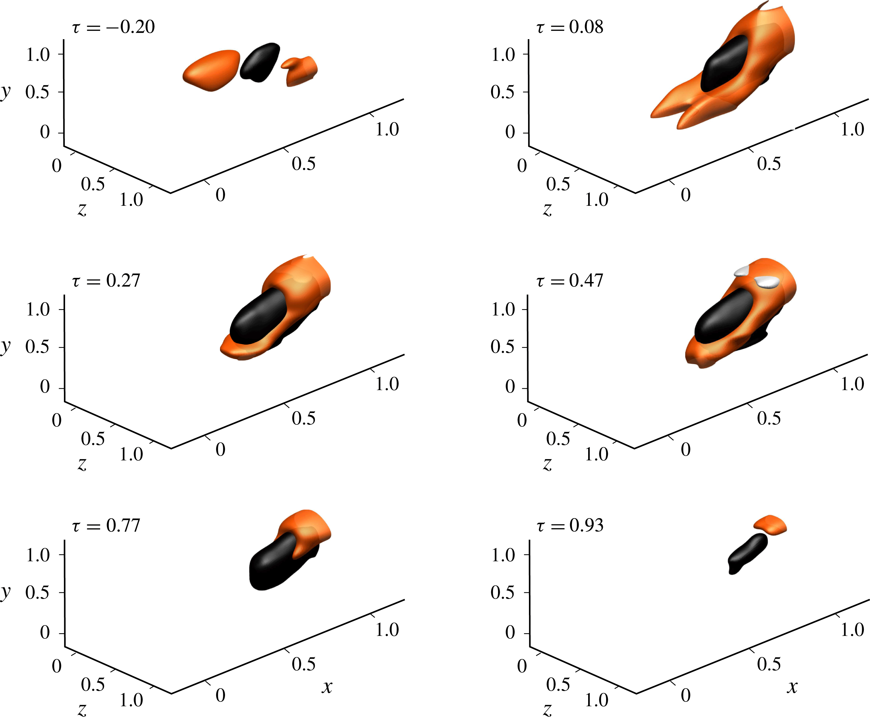
The dynamically averaged turbulent hairpin process. Isosurfaces of positive (white) and negative (black) streamwise velocity fluctuations
 $u^{\prime }$
with isosurfaces of the
 $Q$
criterion (red) at selected time instants. An animation (see movie 3) is available as part of the supplementary material.

The analysis is based on approximately 2700 sampled hairpins and represents, to the best of our knowledge, the first time-resolved statistical characterization of the hairpin process in a natural turbulent shear flow. So as to make the approach more robust against the erroneous identification of structures that momentarily pass the topological filter, only structures that persist for more than 0.05 time units are considered. In this context, we wish to emphasize that the conditioning applied in the analysis only concerns the
 $Q$
field, which, after being condensed into a discrete graph as described in § 3, was topologically filtered with the criteria detailed in table 1. On the other hand, the velocity field is not subject to any constraints and, as such, its average emerges naturally as a consequence of the conditioning applied to the
 $Q$
criterion.
Results for the dynamically averaged evolution of the turbulent hairpin are presented in figure 26. The choice of an initial time that precedes the formation of the arc-shaped structures provides insight into the origin of the turbulent hairpin process. At
 $\unicode[STIX]{x1D70F}=-0.20$
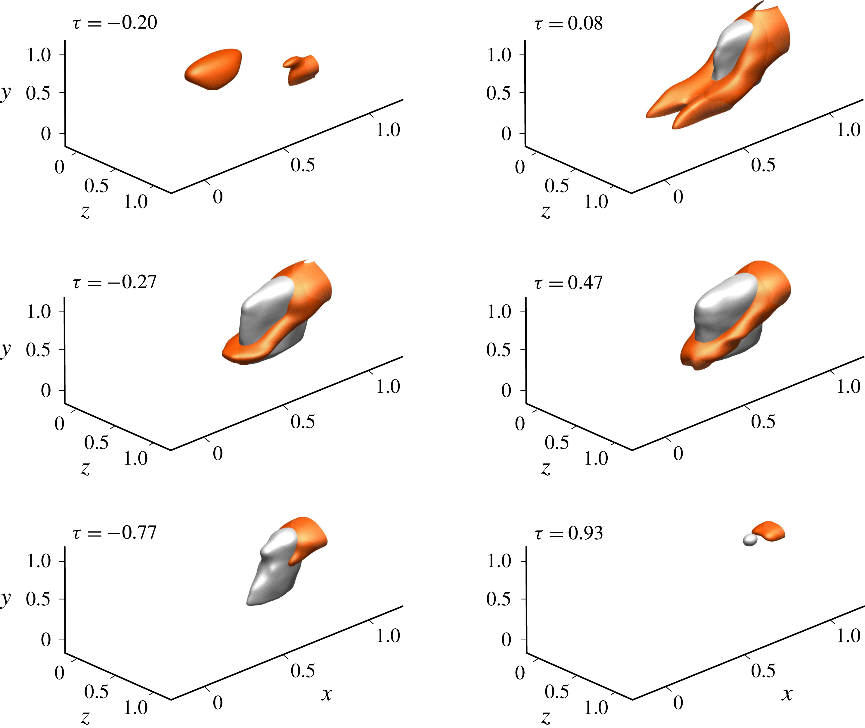
, i.e. 0.20 normalized lifetimes before the hairpins become discernible in the flow, a patch of negative streamwise velocity fluctuations resides at the centre of the sampling domain. As the hairpins form and evolve, this patch is amplified and increases in extent. Normal fluctuations, visualized in figure 27, are initially largely absent. During the lifetime of the hairpin, a localized ejection, represented by a patch of positive
 $v^{\prime }$
, is generated at the centre.
The dynamically averaged turbulent hairpin process. Isosurfaces of positive (white) and negative (black) normal velocity fluctuations
 $v^{\prime }$
with isosurfaces of the
 $Q$
criterion (red) at selected time instants. An animation (see movie 4) is available as part of the supplementary material.

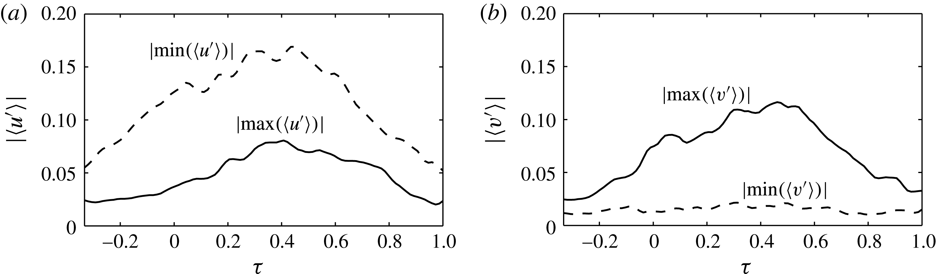
The absolute extrema within the normalized sampling domain are presented in figure 28 as a function of the normalized lifetime,
 $\unicode[STIX]{x1D70F}$
. Similarly to the mechanism governing the hairpins in the late transitional flow, the centre region of the turbulent hairpins is associated with an amplification of negative
 $u^{\prime }$
and positive
 $v^{\prime }$
. In contrast to algebraic growth, which is characterized by a delayed amplification of
 $u^{\prime }$
following an initial
 $v^{\prime }$
perturbation (see, e.g., Hultgren & Gustavsson Reference Hultgren and Gustavsson1981), the two components are amplified simultaneously, providing further evidence for the presence of an exponential instability mechanism. In particular, the analysis of the turbulent hairpin also lends additional support to the reported connection to energetic ejection events.
Absolute values of the maximum (solid) and minimum (dashed) dynamically averaged velocity fluctuations within the sampling domain as a function of sampling time. (a) Streamwise fluctuations. (b) Normal fluctuations.

5.3 Statistical results
Beyond the computation of a dynamically averaged process, the data gained in the application of the identification scheme to the turbulent boundary layer also provide rich statistical information about the hairpin process. In the following, we seek to further characterize the turbulent hairpin through a set of statistical results.
Probability density functions (PDFs) of the minimum and maximum streamwise velocity fluctuations are presented in figure 29. The highest amplitudes are observed for the negative streamwise component, whose distribution peaks at around
 $u^{\prime }=-0.06$
. In contrast, the positive streamwise fluctuations have on average appreciably lower amplitudes, with a peak near
 $u^{\prime }=0.02$
. These observations are consistent with the concept of the hairpin being a secondary instability of a negative streamwise velocity fluctuation caused by an earlier event such as the algebraic amplification of small disturbances. The PDFs of the normal component in figure 30 indicate lower amplitudes than in the streamwise fluctuations as well as appreciably narrower distributions.
Probability density functions of the extremal levels of streamwise fluctuations for the sampled hairpins. (a) Minimum fluctuations. (b) Maximum fluctuations.

Probability density functions of the extremal levels of normal fluctuations for the sampled hairpins. (a) Minimum fluctuations. (b) Maximum fluctuations.

Trajectories of the centre positions of identified hairpin structures versus
 $x$
and
 $y$
(a) and
 $y^{+}$
(b). The grey line indicates the local boundary layer thickness.

The spatial organization of the hairpin process within the shear layer has been the subject of open debate. The currently perhaps best established position was put forward in the review by Adrian (Reference Adrian2007), who postulated that the boundary layer would be populated by a hierarchy of hairpins. Other researchers, including Schlatter et al. (Reference Schlatter, Li, Örlu, Hussain and Henningson2014), were more critical and suggested that the hairpin process would be limited to the outermost regions of a shear layer. The trajectories of the streamwise and normal positions gained in the present analysis are presented in figure 31. Circles mark the initial and final positions of the identified structures and lines indicate the paths of their centres, defined as the mean wall distance and streamwise position. As with the computation of the dynamic average, only structures that persist for more than 0.05 time units are considered, which makes the approach more robust against the misidentification of flow features that instantaneously pass the topological filter.
In terms of the physical scaling of the wall distance presented in figure 31(a), the density of the trajectories suggests a nearly homogeneous population of the boundary layer by hairpins. The structures occupy a region ranging from the wall to the edge of the turbulent boundary layer, defined as the location where the mean velocity profile reaches 99 % of its free-stream value. Only a spurious number of samples are found beyond this demarkation. The evaluation is repeated in figure 31(b) based on a normal coordinate in wall units. In this scaling, the viscous region near the wall,
 $y^{+}\lesssim 5$
, is free from trajectories throughout the computational domain. Although the results show a clear concentration of structures near the edge of the boundary layer, the buffer layer,
 $10\lesssim y^{+}\lesssim 30$
, also hosts an appreciable number of hairpins.
A more differentiated picture emerges when considering the lowest point of the medial axis of each individual hairpin as opposed to the centre positions evaluated above. Figure 32(a) shows the traces of the locations closest to the wall of the fifth of all hairpins located farthest away from the wall, demonstrating that these structures remain limited to the outer regions of the shear. In contrast, the lowest point of the quintile of the population closest to the wall (figure 32
b) is largely confined to the buffer layer, with single structures reaching as far as
 $y^{+}\approx 2$
into the viscous sublayer. Taken as a whole, these results do not support the notion of the hairpins originating at the wall and subsequently rising through the boundary layer. They rather indicate that the hairpins are generated at different heights which they largely maintain during their lifetime.
Trajectories of the locations closest to the wall of identified hairpin structures versus
 $x$
and
 $y^{+}$
. The fifth of the population located farthest from the wall (a) and the fifth of the population located closest to the wall (b).

Probability density function of the frequency of occurrence of hairpin structures. (a) As a function of the streamwise coordinate. (b) As a function of the dimensionless wall distance.

Probability density functions relate the frequency of occurrence of hairpins to the streamwise location in figure 33(a). A noteworthy outcome is the near-constant level of the PDF past the initial growth at the onset of turbulence. The slow decay farther downstream may likely be attributed to the increasing distortion of the individual flow structures at higher Reynolds numbers. The frequency of occurrence as a function of the wall distance is presented in figure 33(b). The distribution shows a maximum near
 $y^{+}\approx 80$
and decays towards larger wall distances.
The scaling of the spatial extent of the hairpin process is examined by defining a characteristic length scale in terms of the mean spanwise width in wall units,
 $\unicode[STIX]{x0394}z^{+}$
, averaged over the lifetime of each individual hairpin. When considering the influence of the streamwise coordinate on
 $\unicode[STIX]{x0394}z^{+}$
, the expansion of the boundary layer suggests a moderate growth of the largest scales. On the other hand, the reduction in the friction velocity
 $u_{\unicode[STIX]{x1D70F}}$
and the increase in the Reynolds number support a decrease of the mean length scales in wall units. Results presented in figure 34(a) show a marginally positive correlation between
 $x$
and
 $\unicode[STIX]{x0394}z^{+}$
and indicate that, for the considered range of moderate Reynolds numbers, the former effect outweighs the latter.
When considering the scaling of flow structures with wall distance, the hairpin model by Adrian (Reference Adrian2007) suggests a hierarchy of structures whose length scales increase with wall distance. The present results point to a largely linear relation between
 $y^{+}$
and
 $\unicode[STIX]{x0394}z^{+}$
(see figure 34
b) and hence support this aspect of the model. In particular, the results substantiate the compatibility of the hairpin process with the general attached-eddy hypothesis introduced by Townsend (Reference Townsend1961), which predicts the scaling of flow structures with wall distance.
Histogram of the spanwise extent of hairpin structures. (a) As a function of the streamwise coordinate and the physical wall distance. (b) As a function of the streamwise coordinate and the dimensionless wall distance.

Finally, the temporal scaling of the hairpin process in the boundary layer in the form of its mean lifetime,
 $\unicode[STIX]{x0394}t$
, is considered. Physical arguments support trends consistent with those observed for the spatial scaling. The relation between the streamwise position and the average lifetime of all samples located there is presented in figure 35(a), pointing to a weakly positive correlation similar to the spatial scaling. The mean lifetime grows more quickly with
 $y^{+}$
(figure 35
b) while following a largely linear trend.
Histogram of the lifetime of hairpin structures. (a) As a function of the streamwise coordinate and the physical wall distance. (b) As a function of the streamwise coordinate and the dimensionless wall distance.

6 Conclusions
An investigation into the mechanism driving the hairpin process in transitional and turbulent flow was presented. Information on the hairpin process was extracted from direct simulation data using a topological algorithm. The results were complemented by linear stability analyses. The outcome relates the coherent hairpin structure to a coherent instability mechanism which at its core is governed by linear theory. Nonlinear effects nonetheless play a meaningful role in altering and reshaping the linear eigensolutions. A comparison between the transitional and turbulent hairpins shows fundamentally consistent trends and thus substantiates earlier hypotheses of commensurate physics.
A topological algorithm for the time-resolved identification and analysis of arbitrary coherent dynamical flow processes was introduced. The methodology is based on concepts developed in the fields of computer vision and image processing. It distils the structure of arbitrary field quantities into a graph described by sets of discrete links and nodes. Application of topological filtering criteria to the graph allows the isolation of specific classes of flow structures. One of the advantages of the method lies in its ability to identify equivalent flow processes across multiple scales while preserving temporal causality. Within the scope of this work, the framework enabled the time-resolved analysis of the transitional and turbulent hairpin processes.
The hairpins observed in the late stages of transition to turbulence can be described as extreme events based on the magnitudes of the perturbations that are generated. Enstrophy as well as production and dissipation of perturbation kinetic energy show instantaneous peaks which appreciably exceed the levels observed in fully turbulent flow. Specifically, the absence of turbulence and the associated transport of momentum likely explain why the transitional hairpin is able to attain exceptional levels of kinetic energy. The most highly energetic perturbations are spatially localized in the tip or head of the arc-shaped hairpin structure. Analysis of the temporal evolution of the perturbation amplitudes showed a clearly exponential trend. Further evidence for the presence of an exponential instability was gained from visualizations of the instantaneous critical layer, which proved to be aligned with the tip of the hairpin.
Linear stability analysis confirmed the presence of an exponential instability which coincides with the formation of the transitional hairpin structure. Prior to the interval of rapid exponential growth, the amplification of disturbances during the earlier stages of the transition process generates an intense localized patch of low-momentum fluid. The resulting distortion of the boundary layer makes the flow susceptible to an inviscid instability mechanism that is captured by linear stability theory. The primary eigenfunction computed in the stability analysis is of varicose type and can be interpreted as a higher instability of the pre-existing perturbation of the boundary layer. Notably, an evaluation of the
 $Q$
criterion for the eigenfunction produces an elementary rendition of the nonlinear hairpin structure. From this perspective, the transitional hairpin as visualized through vortex identification criteria can be interpreted as a symptom of an instability mechanism precipitated by a pre-existing distortion of the boundary layer. Although the instability is at its core a linear mechanism, the high amplitudes of the disturbances imply that nonlinear effects play an appreciable role in modulating and reshaping the linear solution.
Ample evidence for the formation of characteristic packets of hairpins is found in the literature. The present results show that the generation of the packet in transitional flow occurs in a self-similar process that is accompanied by the streamwise splitting of the same patch of low-velocity fluid which also gives rise to the primary hairpin. As the latter breaks away, a second hairpin is generated upstream and eventually also separates from the remaining patch. The length scales of the splitting increasingly shorten until the flow locally breaks down to turbulence. The breakup of the initially homogeneous patch through the generation of a streamwise alternating pattern of increased and decreased intensity is again consistent with a varicose instability. In particular, the length scales are comparable with those of the eigenfunction. As such, it stands to reason that while nonlinear effects can again be expected to appreciably affect the outcome, at its core, the packet formation can as well be traced to a linear mechanism.
Downstream of the transitional regime, the chaotic conditions of turbulence render the analysis of individual flow processes an incomparably more challenging task, not only from a methodological perspective but also in terms of the significance and universality of the gathered results. In a first step, the identification algorithm was applied to the study of the time evolution of an individual hairpin in turbulent flow. The results showed trends that are commensurate with the transitional hairpin as well as with earlier studies of the turbulent hairpin process. The arch of the hairpin structure encloses a region of low-momentum fluid, while the surrounding fluid has an increased streamwise velocity. Perhaps more importantly, the centre region also hosts a patch of highly energetic fluctuations directed away from the wall, supporting the link between the hairpin process and ejection and burst events. Linear analyses provided a further analogy to the transitional flow in the form of a varicose instability eigenfunction that coincides with the early stages of the turbulent hairpin.
Statistical relevance was gained by complementing the study of the individual turbulent hairpin with data acquired in the sampling of several thousand hairpin events. The data were processed to compute a dynamically averaged hairpin which preserves temporal causality. The trends observed during the evolution of the averaged hairpin process are in qualitative agreement both with the individual turbulent hairpin and the transitional hairpins. The averaged turbulent hairpin process too is preceded by a patch of negative streamwise velocity fluctuations, which causes the amplification of normal and streamwise perturbations on a relatively short streamwise length scale. These findings provide further support to the premise of the hairpin being a manifestation of a secondary instability due to a pre-existing distortion of the boundary layer.
Beyond the computation of a dynamic average, the sampling of a large number of turbulent hairpins also provided extensive statistical data. The trajectories of the hairpins show that they largely maintain their normal position within the boundary layer without significant changes in their distance from the wall. With the exception of the near-wall region,
 $y^{+}\lesssim 10$
, the hairpin process was identified throughout the largest part of the turbulent boundary layer. Both the spatial and the temporal scales increase with distance from the wall. As such, the present results support earlier accounts of the compatibility of the hairpin with the attached-eddy hypothesis of Townsend (Reference Townsend1961).
Overall, the results presented in this study provide strong support for a connection between the transitional and turbulent hairpin processes. Both classes show a comparable signature in the velocity field. They are preceded by a distortion of the mean flow which in the transitional case can be attributed to the exponential growth of disturbances such as Tollmien–Schlichting waves. In the turbulent regime, the origin of the distortion is more likely related to algebraic growth mechanisms such as Orr and lift-up. The transitional hairpin process may thus be considered as a prototype of its turbulent counterpart.
In terms of the causality of events, the results indicate that the hairpin is an outcome of the modulation of the shear layer by an earlier event which makes the flow susceptible to the amplification of inviscid instabilities. This explanation implies that the patch of low-momentum fluid at the centre of the hairpin is not primarily an outcome of the hairpin itself, although the latter may contribute to it. The link between the hairpin process and an exponential instability mechanism explains the statistical preference of the hairpin compared with other realizable structures throughout a range of wall-bounded shear flows and hence its nature as a coherent structure. In particular, the arc-shaped structure itself as observed in visualizations of vortex identification criteria can be seen as a manifestation of the varicose nature of the instability.
Acknowledgements
The authors wish to thank C. W. Hamman for generating the DNS time series of the boundary layer used in the analysis, and the insightful comments of three anonymous referees. This work was supported by the Office of Naval Research, the Air Force Office of Scientific Research and Deutsche Forschungsgemeinschaft.
Supplementary movies
Supplementary movies are available at https://doi.org/10.1017/jfm.2018.202.