1. Introduction
With the increasing safety, flexibility and maneuverability of UAVs in recent years, their applications are no longer limited to research institutes and industry sectors, and the scale of commercial UAVs in public grows rapidly [Reference Floreano and Wood1]. However, due to some misuse and malicious operations, reports of UAVs intruding into airports, rail lines and high-traffic areas are becoming more common. How to effectively approach and intercept these small aerial targets is now a well-attended research topic. Existing solutions mainly include UAV remote control or positioning signal jamming and physical shootdown [Reference Farid, Kuan, Kamal and Wong2]. However, anti-UAV devices generally have limited effective ranges, and physical interception can easily cause secondary damage. To address these issues, we study an aerial interception scheme that employs UAVs to autonomously track and intercept intruding targets.
The limited load and computing capabilities of UAVs make it difficult to carry heavy sensors and run complex navigation algorithms [Reference Hassanalian and Abdelkefi3]. Thus, vision sensors and vision-based control methods receive more and more attention in UAV autonomous flight tasks [Reference Xie, Lynch and Jagersand4–Reference Gao8]. Among these methods, image-based visual servoing (IBVS) approaches, which directly rely on error signals in the image plane and do not require accurate modeling of the camera and target [Reference Hutchinson, Hager and Corke9, Reference Chaumette and Hutchinson10], have been proved an effective solution to the target tracking problem for UAVs. In ref. [Reference Abdessameud and Janabi-Sharifi11], an image-based control scheme of an UAV is proposed for tracking a planar motion target with the assumption that external disturbances are constant. This theoretical result is extended to time-varying external disturbances in ref. [Reference Asl12]. Using a nonlinear velocity observer, an IBVS controller for tracking a visual target in a tilted plane can be found in ref. [Reference Zheng, Wang, Wang, Chen, Chen and Liang13]. Similarly, a visual servoing method is presented in ref. [Reference Li, Xie, Low, Yong and Li14], which can be applied to track an arbitrarily oriented planar target. Furthermore, to intercept targets flying in the air, an IBVS algorithm is provided in ref. [Reference Yang and Quan15] using a simplified rigid body dynamics model. Then, in ref. [Reference Wang, Qin, Liu, Ma and Zhang16], by adopting a virtual camera approach, an image-based tracking scheme that considers the full dynamics model of the UAV is proposed for arbitrary motion targets in three dimensional (3D) space. However, because of the limited FOV of onboard cameras, the works mentioned above all assume that the target is always detectable during tracking process. In practical scenarios, in order to avoid the target loss, the UAVs are usually limited in flight speed.
There have been various works to address the target-loss problem. In ref. [Reference Heshmati-alamdari, Karras, Eqtami and Kyriakopoulos17], an IBVS-model predictive control approach is proposed for mobile robot visual tracking, which formulates visibility constraints as state constraints. Using an error transformation to incorporate the desired performance specifications, two leader-following tracking controllers for mobile robots is developed in ref. [Reference Miao, Zhong, Lin, Wang, Chen and Fierro18] without violating the FOV constraints. Then, by planning a smooth trajectory in image space, a control scheme is presented in ref. [Reference Zheng, Wang, Chen and Wang19] to improve visibility during the UAV visual servoing process. To avoid losing the image feature, a Q-learning algorithm is adopted in ref. [Reference Shi, Shi, Sun and Hwang20] to adaptively adjust the servoing gain for IBVS control of quadrotors. This work is modified in ref. [Reference Jin, Wu, Liu, Zhang and Yu21] by using the deep deterministic policy gradient algorithm to select the gain in a continuous space. However, these algorithm-level improvements are difficult to achieve satisfactory results in the aerial interception scenarios with target maneuvers.
Motivated by the aforementioned limitations, we employ the camera network as the external sensing module of the aerial interception system. Due to its unlimited FOV, the network can effectively sense any aircraft that enters the surveillance area and avoid the loss of the target with evasive motion. Besides, the interceptor UAV does not need to carry environmental sensors, which can reduce its computational burden and increase the flight speed.
Camera networks have been extensively studied over the past few decades. Utilizing optimization methods, early works focus on coverage and monitoring of typical areas with the minimum number of cameras [Reference Akyildiz, Melodia and Chowdhury22, Reference Cheng and Savkin23]. Then, some distributed control approaches are presented in refs. [Reference Song, Ding, Kamal, Farrell and Roy-chowdhury24–Reference Zhang, Qin, Li, Wang, Wang and Zheng26] to enable mobile sensors to continuously track multiple moving objects in the surveillance region. However, the existing works are dedicated to improving surveillance performance of camera networks, but ignore the significant potential of their broad FOV for UAV detection and localization. Although in ref. [Reference Zheng, Zheng, Zhang, Chen, Chen and Zhao27], a systematic approach is proposed to detect and track multiple UAVs simultaneously. Because of adopting special panoramic stereo cameras, it is difficult to apply in practical scenarios where only ordinary cameras are installed.
In this paper, we propose a novel eye-to-hand vision-based control scheme that drives an quadrotor UAV to track and intercept an aerial object based on a ground visual sensor network. The quadrotor is equipped with only an inertial measurement unit (IMU) and a global positioning system (GPS) receiver, and its perception of environment relies on the sensor network. In particular, a visual servoing equation is formulated using rotation matrices and pinhole camera models. As a result, the relationship of the aircraft motion in image space and Cartesian space is presented to simplify the control design. Then, directly based on error signals in image planes of camera nodes, an IBVS controller is designed such that a stable and efficient interception is achieved. Finally, the effectiveness of our method is verified by experiments in both simulated and real environments.
The contributions of this paper are summarized as follows:
-
• To the best of our knowledge, this is the first work that adopts ground camera network for image-based control to aerial interception of UAVs.
-
• Because the control values are computed directly based on image errors of camera nodes, the proposed approach is insensitive to errors due to camera modeling and calibration. As a result, wide-angle lens cameras can be applied to provide greater FOV coverage.
-
• By fusing the control signals of multiple camera nodes, the system is robust against the appearance change of targets due to illumination and occlusion and could cover a larger area for longer distance tracking and interception.
-
• In addition to enabling rear tracking of aerial objects [Reference Li, Ning, He, Lee and Zhao6, Reference Yang and Quan15, Reference Wang, Qin, Liu, Ma and Zhang16], our method can achieve forward interception of these targets. Both simulations and outdoor experiments validate the efficient interception.
The remainder of this paper is organized as follows. Section 2 presents the architecture of our aerial interception system. Section 3 describes the visual servoing model, and Section 4 details the vision-based controller design and analyzes the system stability. Experimental results obtained through simulated and actual flight tests are shown in Section 5, and this paper is concluded in Section 6.
2. System overview
2.1. Problem description
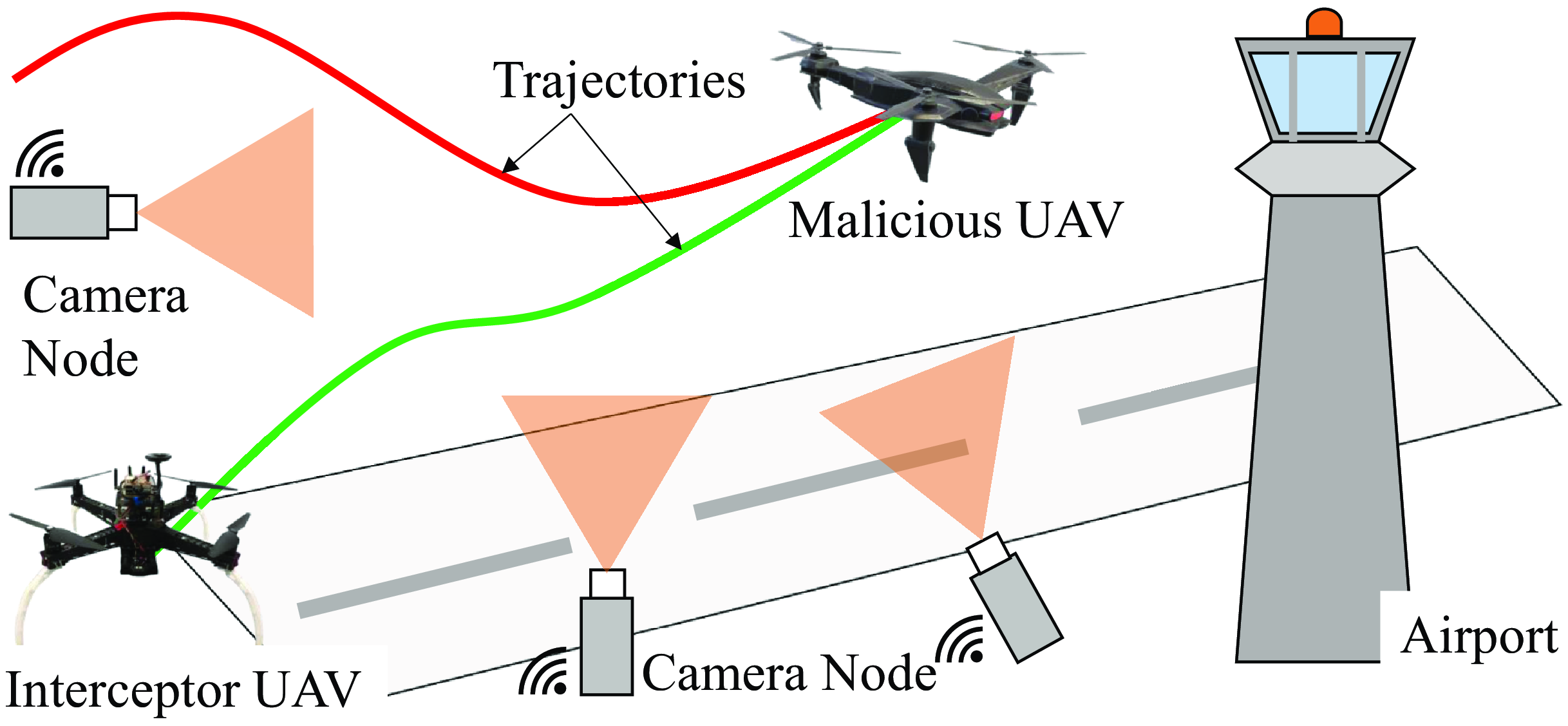
Our UAV intercepting malicious UAV that disrupts airport. The green and red curves indicate the flight trajectories of the UAVs. The interceptor UAV does not have any sensors installed to detect the target UAV and all of its control signals come from the ground visual sensor network.

A camera network-based aerial interception system consists of a ground surveillance network and an interceptor quadrotor UAV. When a malicious air target is detected by the camera nodes in the network, an eye-to-hand IBVS controller drives the UAV to track and intercept the target (see Figure 1). In this paper, we consider the control objective to be achieved when the interceptor UAV keeps approaching the aerial target until the Euclidean distance between them is less than a fixed threshold. The interceptor UAV is equipped with only an IMU and a GPS receiver, and all of its control signals are generated from the image errors of the visual sensor network.
For complete interception, perception and localization as well as control modules are essential. In this paper, we focus on the most fundamental and challenging part, which is the control technique. We adopt the efficient approaches on detection [Reference Barnich and Van Droogenbroeck28] and state estimation [Reference Mahony, Kumar and Corke29]. The surveillance range of the aerial interception system is primarily determined by the visual perception module. Its limits mainly include: a) quantity, b) spatial arrangement and c) FOV coverage of camera nodes in the visual sensor network. To achieve the control objective, we have the following assumption.
Assumption 1. During interception, at least two camera nodes in the visual sensor network can perceive both the interceptor and the target at the same time.


2.2. Implementation architecture
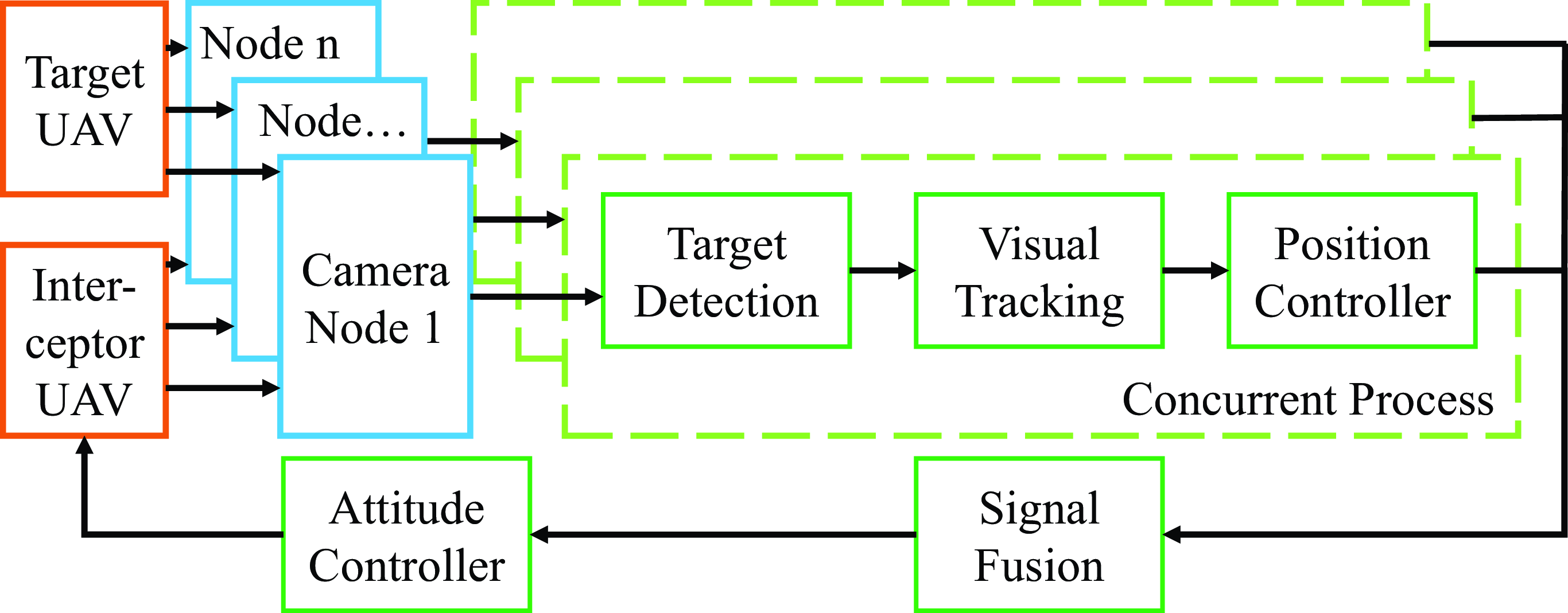
Architecture of the proposed camera network-based aerial interception system.

The framework of the interception system is exhibited in Figure 2. In this paper, the cameras in the considered network are fixedly installed on the ground (i.e., eye-to-hand, the onboard vision sensor is eye-in-hand). Therefore, we use a background subtraction algorithm [Reference Barnich and Van Droogenbroeck28] to detect and track the interceptor and target UAV that enter the surveillance area. Then, depending directly on image errors of the camera nodes, we design an IBVS controller to generate the desired velocity of the interceptor quadrotor. In order to improve the interception efficiency, we finally develop low-level attitude controllers to track the desired translational control command and achieve tracking and interception of the malicious target.
Remark 2. It should be noted that as the perception module, the background subtraction algorithm effects the performance of the whole aerial interception system. Although deep learning has made tremendous progress in the field of visual perception in recent years. We still adopt the background subtraction algorithm due to the advantages in processing speed, detection precision and model size.
3. Visual servo model
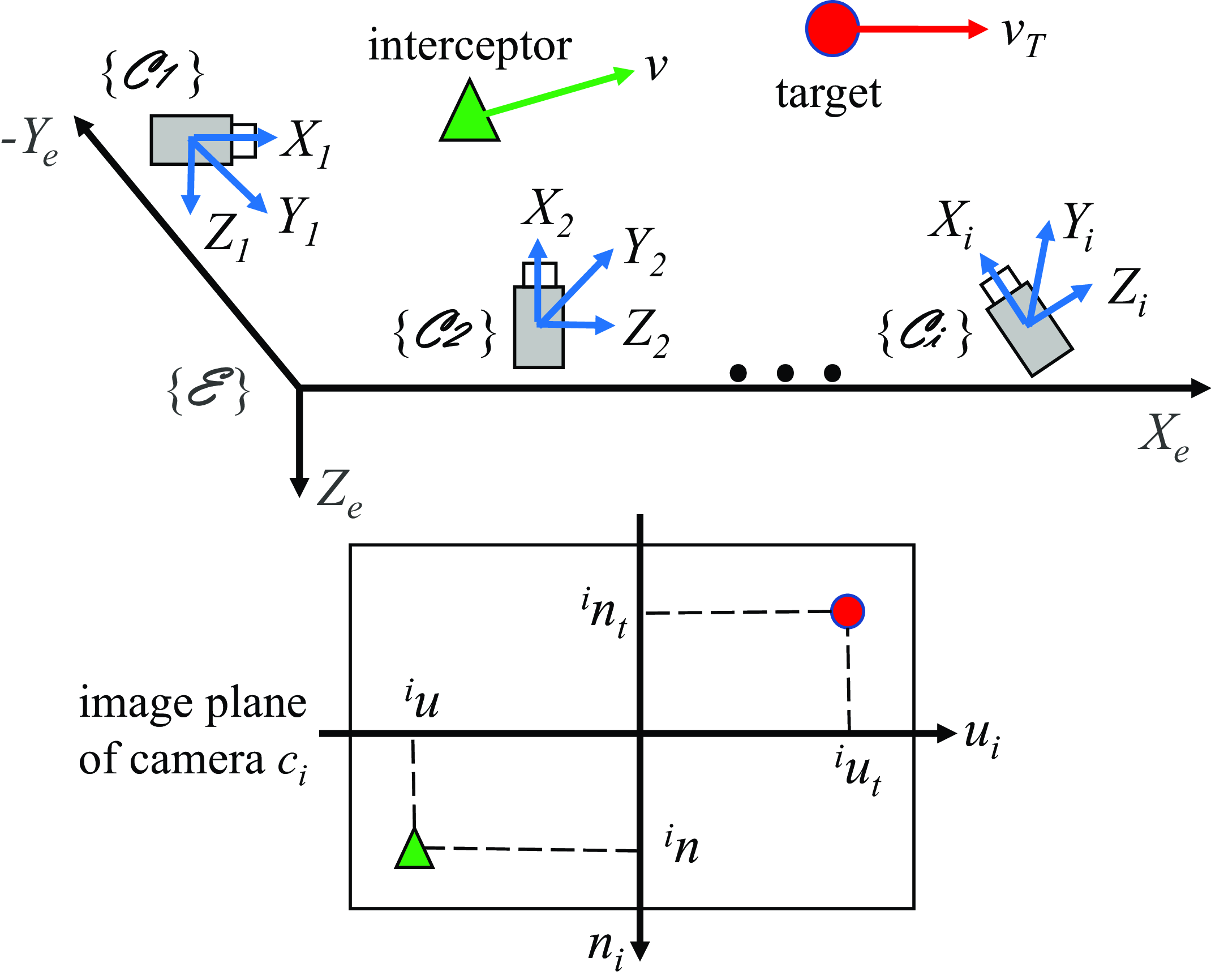
Reference frames and image plane considered in this paper. The green triangle and red circle represent the intercepting UAV and aerial target, respectively.

As shown in Figure 3, there is a typical scheme of eye-to-hand visual servoing of the UAV air interception system. The inertial frame
 $\mathcal {E}=\{X_e,Y_e,Z_e\}$
is fixed to the ground and orients north, east and down. Let
 $c_i$
,
 $i \in \mathcal {N} \,:\!= \{1,\ldots, n\}$
, denotes the
 $i$
-th camera node in the visual sensor network. The origin (
 $\boldsymbol{O}_i$
) of the camera frame
 $\mathcal {C}_i=\{X_i,Y_i,Z_i\}$
coincides with the optical center of the camera
 $c_i$
, the
 $X_i$
axis overlap with the optical axis, and the
 $Z_i$
axis is always perpendicular to the
 $X_e$
-
 $Y_e$
plane and directed downwards.
We let
 $\boldsymbol{p} = [x,y,z]^T \in \mathbb {R}^3$
and
 ${^{i}\boldsymbol{p}} = [{^{i}x},{^{i}y},{^{i}z}]^T \in \mathbb {R}^3$
denote the positions of the interceptor UAV in
 $\mathcal {E}$
and
 $\mathcal {C}_i$
, respectively, which satisfies
 \begin{equation} {^{i}\boldsymbol{p}} = \boldsymbol{R}_{i}^{T} (\boldsymbol{p} - \boldsymbol{O}_i) \end{equation}
where
 $\boldsymbol{R}_{i} \in SO(3)$
denotes the rotation matrix that brings
 $\mathcal {C}_i$
into
 $\mathcal {E}$
and is associated with three orientation angles of the camera
 $c_i$
. Note that
 $SO(3)\, :\!= \{\boldsymbol{R} \in \mathbb {R}^{3 \times 3} | \boldsymbol{R}^T\boldsymbol{R} = \boldsymbol{I}_3, det(\boldsymbol{R}) = 1\}$
represents the third-order special orthogonal group. Consider each camera node in the visual sensor network with a fixed position and orientation, then we have
 \begin{equation} {^{i}\dot {\boldsymbol{p}}} = \boldsymbol{R}_{i}^{T} \dot {\boldsymbol{p}} \end{equation}
where
 $\dot {\boldsymbol{p}}$
is the linear velocity of the interceptor in
 $\mathcal {E}$
.
Let
 $[{^{i}u},{^{i}n}]^T \in \mathbb {R}^2$
and
 $[{^{i}u_t},{^{i}n_t}]^T \in \mathbb {R}^2$
represent the coordinates of the interceptor and target in the image plane of the camera
 $c_i$
,
 $i \in \mathcal {N}$
, respectively. Based on a pinhole camera model, we can write
 \begin{equation} {^{i}u} = \lambda _i \frac {^{i}y} {^{i}x}, {^{i}n} = \lambda _i \frac {^{i}z} {^{i}x} \end{equation}
where
 $\lambda _i$
is the focal length of the camera
 $c_i$
,
 $i \in \mathcal {N}$
. Then, the time-derivative of
 $[{^{i}u},{^{i}n}]^T$
can be expressed as
 \begin{equation} \begin{bmatrix} {^{i}\dot {u}} \\ {^{i}\dot {n}} \end{bmatrix} = \left[\begin{array}{c@{\quad}c@{\quad}c} -\dfrac {^{i}u}{^{i}x} & \dfrac {\lambda _i}{^{i}x} & 0 \\ -\dfrac {^{i}n}{^{i}x} & 0 & \dfrac {\lambda _i}{^{i}x} \end{array}\right] \begin{bmatrix} {^{i}\dot {x}} \\ {^{i}\dot {y}} \\ {^{i}\dot {z}} \end{bmatrix} \end{equation}
which establishes the relationship between the changing rates of the coordinates of interceptor in the image plane and the camera frame of
 $c_i$
,
 $i \in \mathcal {N}$
. Note that
 $^{i}x$
can be obtained by (1) using the absolute position of the interceptor UAV from the onboard GPS receiver.
4. Camera network-based visual servo control
This section elaborates the camera network-based tracking control algorithms proposed in this work. First, we develop a velocity controller using the visual servo model derived in Section 3. Then, based on the geometric projection, we fuse the control signals from different camera nodes. Final, in order to accomplish the interception missions efficiently and accurately, a low-level flight controller is designed for the interceptor UAV to achieve the desired velocity command.
4.1. Velocity controller design and stability analysis
In this work, when the interceptor UAV approaches and intercepts the target, the distance
 $d$
between the projections of these two vehicles in the image plane converges to zero. Thus, let us define the control error signal in the image plane of
 $c_i$
,
 $i \in \mathcal {N}$
 \begin{equation} \delta _i = d_i - d_d \end{equation}
where
 $d_i$
and
 $d_d$
denote the real and desired distances from
 $c_i$
, respectively. Based on the above-mentioned facts, we consider that
 $d_d = 0$
, and the image error satisfies
 \begin{equation} \dot {\delta }_i = \dot {d}_i \end{equation}
where
 $d_i = \sqrt {({^{i}u} - {^{i}u_t})^2 + ({^{i}n} - {^{i}n_t})^2}$
. Then, it can be verified that the system (6) is non-autonomous, because
 $\dot {d}_i$
is a function of time
 $t$
instead of
 $\delta _i$
. Consider the following continuously differentiable positive-definite function
 \begin{equation} L_i = \frac 12 {\delta _i}^2 . \end{equation}
Using (4), the time-derivative of
 $L_i$
along the trajectory (6) gives
 \begin{equation} \dot {L}_i = - \left({^{i}u_t} - {^{i}u}\right)\left(\frac {\lambda _i{^{i}\dot {y}} - {^{i}u}{^{i}\dot {x}}}{^{i}x} - {^{i}\dot {u}_t}\right) - \left({^{i}n_t} - {^{i}n}\right)\left(\frac {\lambda _i{^{i}\dot {z}} - {^{i}n}{^{i}\dot {x}}}{^{i}x} - {^{i}\dot {n}_t}\right) . \end{equation}
For fast convergence of the control error
 $\delta _i$
to zero, we consider
 $^{i}\dot {x} = 0$
and choose
 $^{i}\dot {y}$
and
 $^{i}\dot {z}$
as the control inputs. This is reasonable because the
 $X_i$
axis is perpendicular to the image plane, so
 $^{i}\dot {x}$
contributes little to the convergence of the control error. Note that this design doesn’t mean giving up one of the control inputs of the UAV, using rotation matrices, the component of the final control input along the
 $X_e$
axis,
 $\dot {x}$
, will be obtained from
 $^{i}\dot {y}$
and
 $^{i}\dot {z}$
(see Section 4.2).
Then, in view of Eq. (8), we design
 $^{i}\dot {y}$
and
 $^{i}\dot {z}$
such that
 \begin{align} {^{i}\dot {y}} = \frac {k_1{^{i}x}({^{i}u_t} - {^{i}u}) + {^{i}x}{^{i}\dot {u}_t}}{\lambda _i}, \end{align}
 \begin{align} {^{i}\dot {z}} = \frac {k_2{^{i}x}({^{i}n_t} - {^{i}n}) + {^{i}x}{^{i}\dot {n}_t}}{\lambda _i}\\[12pt]\nonumber \end{align}
where
 $k_1, k_2 \gt 0$
are adjustable constants. Eq. (8) then satisfies
 \begin{equation} \dot {L}_i = - k_1({^{i}u_t} - {^{i}u})^2 - k_2({^{i}n_t} - {^{i}n})^2 . \end{equation}
According to [Theorem 4.8, 30],
 $\dot {L}_i$
is negative definite, the system is stable, and the error
 $\delta _i$
in the image plane will converge to zero.
4.2. Signal fusion
According to Assumption1, let
 $c_j$
and
 $c_k$
,
 $j, k \in \mathcal {N}$
, denote the camera nodes which provide effective observation of the interceptor and target at the current moment. Using the control law in the previous subsection, we can obtain the control inputs
 ${^{j}\dot {\boldsymbol{p}}} = [{^{j}\dot {x}},{^{j}\dot {y}},{^{j}\dot {z}}]^T \in \mathbb {R}^3$
and
 ${^{k}\dot {\boldsymbol{p}}} = [{^{k}\dot {x}},{^{k}\dot {y}},{^{k}\dot {z}}]^T \in \mathbb {R}^3$
from
 $c_j$
and
 $c_k$
, respectively. Based on the geometric projection, the fused control command can be calculated as
 \begin{equation} \boldsymbol{v}_{d} = \begin{bmatrix} \dot {x} \\ \dot {y} \\ \dot {z} \end{bmatrix} = \boldsymbol{R}_{j} \begin{bmatrix} {^{j}\dot {x}} \\ \dfrac {{^{k}\dot {y}}\cos \alpha - {^{j}\dot {y}}}{{\cos \alpha }^2 - 1} \\ {^{j}\dot {z}} \end{bmatrix} + \boldsymbol{R}_{k} \begin{bmatrix} {^{k}\dot {x}} \\ \dfrac {{^{j}\dot {y}}\cos \alpha - {^{k}\dot {y}}}{{\cos \alpha }^2 - 1} \\ {^{k}\dot {z}} \end{bmatrix} \end{equation}
where
 $\boldsymbol{v}_{d} \in \mathbb {R}^3$
is the desired linear velocity of the interceptor UAV in the inertial frame
 $\mathcal {E}$
,
 $\boldsymbol{R}_{j}, \boldsymbol{R}_{k} \in SO(3)$
denote the rotation matrices that bring
 $\mathcal {C}_j, \mathcal {C}_k$
into
 $\mathcal {E}$
, respectively, and
 $\alpha$
is the angle between the image planes of
 $c_j$
and
 $c_k$
.
Positions of two objects (represented by green triangle and red circle) in 3D space and their projections in image planes. (a) Coincide in one image plane and separate in 3D space, and (b) coincide in two different image planes and coincide in 3D space.

Remark 3. As shown in Figure 4, it should be noted that when the projections of two objects in different planes all coincide, these objects also coincide in 3D space. Therefore, when each control component
 $^{i}\dot {\boldsymbol{p}}$
of the actual control input
 $\boldsymbol{v}_{d}$
brings the distance
 $d_i$
in the image plane of
 $c_i$
,
 $i \in \mathcal {N}$
to zero, the Euclidean distance between the interceptor UAV and aerial target will converge to zero, and the desired interception will be achieved.
Remark 4. When an aerial target is perceived by more than two camera nodes all the time, two of the cameras capable of continuous detection and visual tracking will be selected to compute interceptor UAV control commands. Although the actual control input
 $\boldsymbol{v}_{d}$
can be obtained from two camera nodes that provide valid observations, in practice we still consider camera network (multiple cameras) for the following reasons. On the one hand, the camera network is robust against the appearance change of targets due to illumination and occlusion. On the other hand, by fusing the control signals of multiple camera nodes, the system could cover a larger area for longer distance tracking and interception.
4.3. Low-level controller design
The dynamics of a quadrotor described by
 \begin{align} \dot {\boldsymbol{p}} &= \boldsymbol{v} \end{align}
 \begin{align} m \dot {\boldsymbol{v}} &= - mg\boldsymbol{e}_{3} + f\boldsymbol{R}_b\boldsymbol{e}_{3} \end{align}
 \begin{align} \dot {\boldsymbol{R}}_b &= \boldsymbol{R}_b\boldsymbol{sk}(\boldsymbol{\omega }) \end{align}
 \begin{align} \boldsymbol{J} \dot {\boldsymbol {\omega }} &= \boldsymbol {\tau } - \boldsymbol{sk}(\boldsymbol {\omega }) \boldsymbol {J \omega } \end{align}
where
 $\boldsymbol{v} \in \mathbb {R}^3$
represents the linear velocity of the quadrotor expressed in
 $\mathcal {E}$
,
 $m$
denotes the mass of the quadrotor,
 $g$
is the gravity acceleration, and
 $\boldsymbol{e}_{3} = [0, 0, 1]^T$
is a unit vector. Let
 $f$
and
 $\boldsymbol {\tau } \in \mathbb {R}^3$
denote the total thrust and the torque vector in the quadrotor body frame
 $\mathcal {B}$
, respectively, and
 $\boldsymbol{R}_b \in SO(3)$
, the rotation matrix from
 $\mathcal {B}$
to
 $\mathcal {E}$
, represents the attitude of the vehicle. Let
 $\boldsymbol {\omega } \in \mathbb {R}^3$
be the angular velocity in
 $\mathcal {B}$
, and
 $\boldsymbol{J} \in \mathbb {R}^{3 \times 3}$
is the inertial moment matrix. The notation
 $\boldsymbol{sk}(\boldsymbol {\cdot })$
denotes the skew-symmetric matrix such that for any vectors
 $\boldsymbol{a}$
,
 $\boldsymbol{b} \in \mathbb {R}^3$
,
 $\boldsymbol{sk}(\boldsymbol{a})\boldsymbol{b} = \boldsymbol{a} \times \boldsymbol{b}$
.
We now design the control inputs
 $f$
and
 $\boldsymbol {\tau }$
to track the desired velocity
 $\boldsymbol{v}_{d}$
. First, using (14), the desired total thrust direction satisfies
 \begin{equation} \boldsymbol{z}_d = \frac {\dot {\boldsymbol{v}}_{d} + g\boldsymbol{e}_{3}} {\Vert \dot {\boldsymbol{v}}_{d} + g\boldsymbol{e}_{3}\Vert } . \end{equation}
During the interception process, to monitor or capture the target, the quadrotor’s heading is expected to be consistent with the direction of the desired velocity
 $\boldsymbol {\sigma } = \boldsymbol{v}_{d} / \Vert \boldsymbol{v}_{d} \Vert$
, which is aligned with the aerial target. Then, we can write
 \begin{equation} \boldsymbol{y}_d = \boldsymbol{z}_d \times \boldsymbol {\sigma }, \boldsymbol{x}_d = \boldsymbol{y}_d \times \boldsymbol{z}_d . \end{equation}
Thus, the desired rotation matrix
 $\boldsymbol{R}_d = [\boldsymbol{x}_d, \boldsymbol{y}_d, \boldsymbol{z}_d]$
can be obtained.
Next, we calculate the total thrust. Define the linear velocity error as
 \begin{equation} \boldsymbol {\delta }_v = \boldsymbol{v} - \boldsymbol{v}_{d} . \end{equation}
Consider the following Lyapunov candidate function
 \begin{equation} L_v = \frac 12 {\boldsymbol {\delta }_{v}}^T \boldsymbol {\delta }_{v}. \end{equation}
By using (14) and the time-derivative of (19), the derivative of
 $L_v$
gives
 \begin{equation} \dot {L}_v = {\boldsymbol {\delta }_{v}}^T \left(\frac fm \boldsymbol{R}_b\boldsymbol{e}_{3} - g\boldsymbol{e}_{3} - \dot {\boldsymbol{v}}_{d}\right) . \end{equation}
We design the control input
 $f$
as
 \begin{equation} f = m (\dot {\boldsymbol{v}}_{d} + g\boldsymbol{e}_{3} - k_3 \boldsymbol {\delta }_v) {\boldsymbol{e}_{3}}^T {\boldsymbol{R}_{b}}^{-1} \end{equation}
where
 $k_3$
is a positively defined parameter. Then, we have
 \begin{equation} \dot {L}_v = - {\boldsymbol {\delta }_{v}}^T k_3 \boldsymbol {\delta }_{v} \end{equation}
which is negative definite and guarantees that
 $\boldsymbol {\delta }_v$
converges to zero.
Final, we utilize a control torque to track the desired attitude
 $\boldsymbol{R}_d$
. The tracking error and angular velocity error are given by
 \begin{align} \boldsymbol {\delta }_R &= \frac 12 ({\boldsymbol{R}_{b}}^T \boldsymbol{R}_{d} - {\boldsymbol{R}_{d}}^T \boldsymbol{R}_{b}) ^ \vee \end{align}
 \begin{align} \boldsymbol {\delta }_\omega &= \boldsymbol {\omega } - {\boldsymbol{R}_{d}}^T \boldsymbol{R}_{b} \boldsymbol {\omega }_d \\[12pt]\nonumber\end{align}
where
 $(\boldsymbol {\cdot }) ^ \vee$
is the inverse operator of
 $\boldsymbol{sk}(\boldsymbol {\cdot })$
and
 $\boldsymbol {\omega }_d$
denotes the desired angular velocity. Then, the time-derivative of
 $\boldsymbol {\delta }_\omega$
satisfies
 \begin{equation} \dot {\boldsymbol {\delta }}_\omega = \dot {\boldsymbol {\omega }} + \boldsymbol{sk}(\boldsymbol {\omega }) {\boldsymbol{R}_{b}}^T \boldsymbol{R}_{d} \boldsymbol {\omega }_d - {\boldsymbol{R}_{b}}^T \boldsymbol{R}_{d} \dot {\boldsymbol {\omega }}_d . \end{equation}
Substituting (16) into (26), motivated by the standard geometric controller [Reference Lee, Leok and McClamroch31], the control input
 $\boldsymbol {\tau }$
can be designed as
 \begin{equation} \boldsymbol {\tau } = - k_R \boldsymbol {\delta }_R - k_\omega \boldsymbol {\delta }_\omega + \boldsymbol{sk}(\boldsymbol {\omega }) \boldsymbol {J \omega } - \boldsymbol{J}[\boldsymbol{sk}(\boldsymbol {\omega }) {\boldsymbol{R}_{b}}^T \boldsymbol{R}_{d} \boldsymbol {\omega }_d - {\boldsymbol{R}_{b}}^T \boldsymbol{R}_{d} \dot {\boldsymbol {\omega }}_d] \end{equation}
where
 $k_R, k_\omega \gt 0$
are adjustable control gains.
Remark 5. It should be noted that the control errors
 $\boldsymbol {\delta }_v$
,
 $\boldsymbol {\delta }_R$
and
 $\boldsymbol {\delta }_\omega$
are computed directly from image features on the image planes of camera nodes. Therefore, the proposed control scheme is insensitive to errors due to camera modeling and calibration, and wide-angle lens cameras can be applied to provide greater FOV coverage.
5. Experiments
To verify the effectiveness of the proposed method, we present a set of experiments in both simulation and real environments in this section. The constant-velocity and varying-velocity targets from different directions are considered to illustrate the tracking and intercepting performance of the system.
5.1. Simulation results
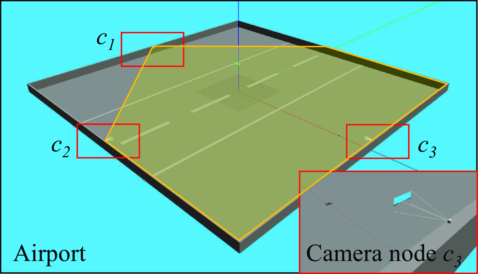
Airport runway environment used in the simulation. The airport is 100 m
 $\times$
100 m, and the wide-angle camera nodes
 $c_1$
,
 $c_2$
,
 $c_3$
are modeled as small cubes. The transparent yellow polygon represents the sensing range of
 $c_1$
in the airport area, blind spots can be seen in the workspace, and the three camera nodes can coverage the entire area.

The simulation scenarios are designed based on the Gazebo simulator, as shown in Figure 5. Two quadrotors, which represent the interceptor UAV and the aerial target, are considered to fly in a 100 m
 $\times$
100 m square area. Although real-world surveillance areas are often larger than those in experiments, such a design can meet the experimental requirements and is conducive to improving the testing efficiency. The origin of the inertial frame is at the center of the area, and the positions of the three wide-angle camera nodes are
 $[-50, 0, 3.5]^T$
m,
 $[0, -50, 3.5]^T$
m and
 $[50, 0, 3.5]^T$
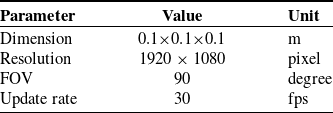
m. Without loss of generality, it is assumed that all camera nodes in the visual sensor network have the same model parameters. The main parameters of the camera nodes are reported in Table I.
In all the simulations in this paper, we adopt the robot operating system (ROS) [Reference Morgan, Conley, Gerkey, Faust, Foote, Leibs, Wheeler and Ng32] as the software framework and the PX4 firmware [Reference Meier, Honegger and Pollefeys33] as the autopilot. The initial positions of the interceptors are
 $[-24.5, -24.5, 0]^T$
m. When an intruding target is perceived by the camera nodes in the sensor network, the proposed algorithm starts running where the control gains
 $k_1 = 5$
,
 $k_2 = 8$
,
 $k_3 = 5.5$
,
 $k_R = 9$
, and
 $k_\omega = 2.5$
. At the same time, the interceptor quadrotor takes off and starts intercepting flight relying on the control signals.
Tracking performance. In this simulation scenario, we consider that the interceptor and target UAVs are initially heading in the same direction. The target quadrotors start from the initial position
 $[-40, 0, 0]^T$
m. In the first simulation, we design a constant-velocity target flying at the velocity
 $[10, 0, 0]^T$
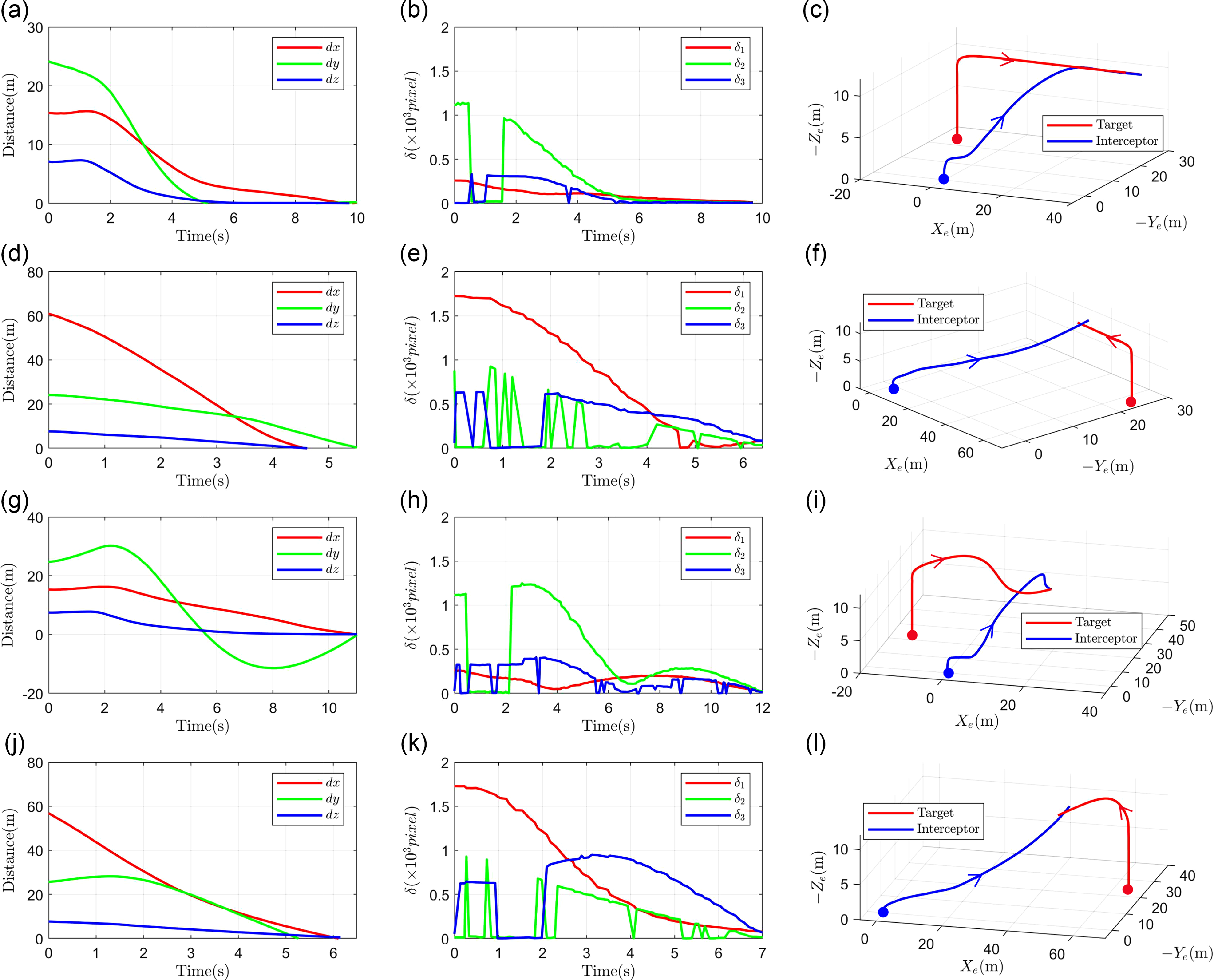
m/s and the altitude 10 m. The time evolution of the distances between the interceptor and target are shown in Figure 6(a). As can be seen, when the distances in
 $X_e$
,
 $Y_e$
and
 $Z_e$
directions converge to zero, the interceptor quadrotor can approach the target. The image error signals from the camera nodes
 $c_1$
,
 $c_2$
and
 $c_3$
are presented in Figure 6(b). Note that the variation of
 $\delta _2$
in the time period of 0.5-1.6 s is due to the fact that the target flies past the interceptor in the image space of
 $c_2$
. The reason why the
 $\delta _3$
curve shows lots of jitter is that during the actual tracking process there are multiple moments when the projections of the interceptor and target coincide in the image plane of
 $c_3$
. Figure 6(c) depicts the trajectories of the interceptor and target during the complete tracking process.
Parameters of camera node in simulation.

Simulation results: distances between interceptor UAV and aerial target, image error signals of camera nodes and flight trajectories. (a), (b), (c) Tracking of a constant-velocity target. (d), (e), (f) Interception of a constant-velocity target. (g), (h), (i) Tracking of a varying-velocity target. (j), (k), (l) Interception of a varying-velocity target. The symbol
 $\bullet$
stand for starting positions.

Also, we consider a varying-velocity target flying along a zigzag trajectory with amplitude of 10 m. The forward speed of the target is 6 m/s. The results obtained from this simulation are presented in Figure 6(g), (h) and (i). As can be seen, the proposed controller is effective for varying-velocity targets in the tracking scenario.
Intercepting performance. In practice, the malicious targets will break into the no-fly zone from arbitrary direction. To demonstrate the satisfying interception capability of our approach, we design the simulation scenario where the target UAVs start from the position
 $[40, 0, 0]^T$
m and fly toward the interceptor. Figure 6(d), (e) and (f) show the simulation results of the constant-velocity target at the velocity
 $[-10, 0, 0]^T$
m/s and the altitude 10 m. And the results of the varying-velocity target are illustrated in Figure 6(j), (k) and (l). All the results indicate that our method can not only achieve tracking behind the targets, but also accomplish interception in front of them.
5.2. Comparison results
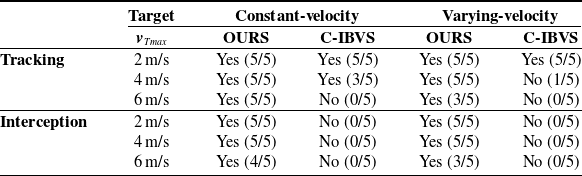
Next, we compare the tracking and interception performance of the proposed scheme with the classic tracking IBVS (C-IBVS) approach [Reference Yang and Quan15] in the airport simulation. In the initialization, we set the same starting positions of the interceptor and target for both methods, but to meet the assumption in ref. [Reference Yang and Quan15], the altitude of the interceptors is set to 10 m, and their orientation is directly towards the target UAVs. To compare the success rates, we design the constant-velocity and varying-velocity targets to fly at maximum speeds of 2, 4, and 6 m/s in the tracking and interception scenarios, respectively. In each of the 5 runs, the initial yaw angle of the target UAV is incremented by 15
 $^\circ$
.
Comparison between [Reference Yang and Quan15] and our method in the airport simulation (successful runs in a total of five runs).

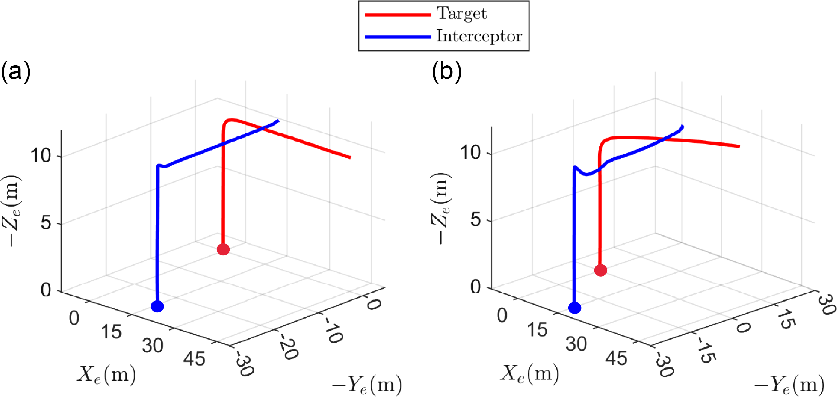
Comparative experiments: flight trajectories for tracking (a) a constant-velocity target and (b) a varying-velocity target using classic tracking IBVS approach proposed in ref. [Reference Yang and Quan15]. The maximum speed of the target is 6 m/s. The symbol
 $\bullet$
stand for starting positions.

The tracking trajectories using C-IBVS are shown in Figure 7. As can be seen, when the aerial target reaches a maximum speed of 6 m/s, the interceptor UAV fails to track and intercept the target satisfactorily even if the target moves with a constant velocity. Target loss in the onboard camera FOV leads to these failures. Hence, the broad FOV of the camera network is necessary for tracking or intercepting varying-velocity targets.
Table II shows all the results of the comparison experiments. In the interception scenario, because the initial position of the target is far away from the interceptor, the onboard camera is unable to make an effective detection, and all of the interceptor UAVs using C-IBVS fail to intercept the targets. In addition, the results in the tracking scenario demonstrate that the C-IBVS method is not able to avoid target loss, especially when the target has maneuverability. It is shown that the proposed approach reduces the target-loss rate by 87.5%. It should be noted that when the target speed is 6 m/s, the target may fly out of the surveillance area before the interceptor UAV approaches it. As a result, the proposed method does not achieve 5/5 successful runs.
5.3. Real experimental results
Hardware devices used in real-world experiments.

Illustration of communication structure in experiment.

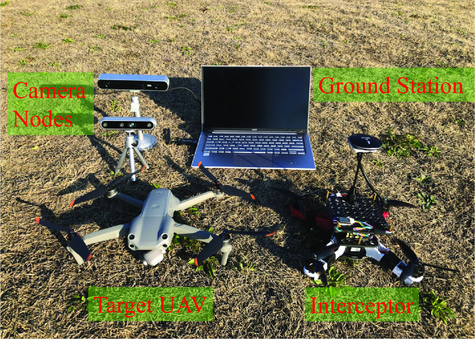
The hardware devices used in the real flight experiments are shown in Figure 8. An Intel Realsense camera and a ZED camera are placed on the ground as the camera nodes. In order to improve maneuverability and facilitate secondary development, we choose a custom-made quadrotor as the interceptor UAV, which uses a 250 mm mainframe, equipped with Formula 32bit 45A electronic speed controllers, T-Motor F60 Pro 2550KV motors and CUAV Pixhawk Nora+ autopilot. A three-axis IMU and a pressure are built into the autopilot, and a CUAV Neo v2 GPS is installed on the top of the drone. To perform high-speed test, HOMER zget data transmitter is used to transfer command data. We use a laptop with an Intel Core i7 CPU, 250G SSD as a ground station to load the camera nodes, run the image detection algorithm and send the intercepting control commands. A DJI Air 2s is adopted as the target object. We use a remote to control the target quadrotor flight.
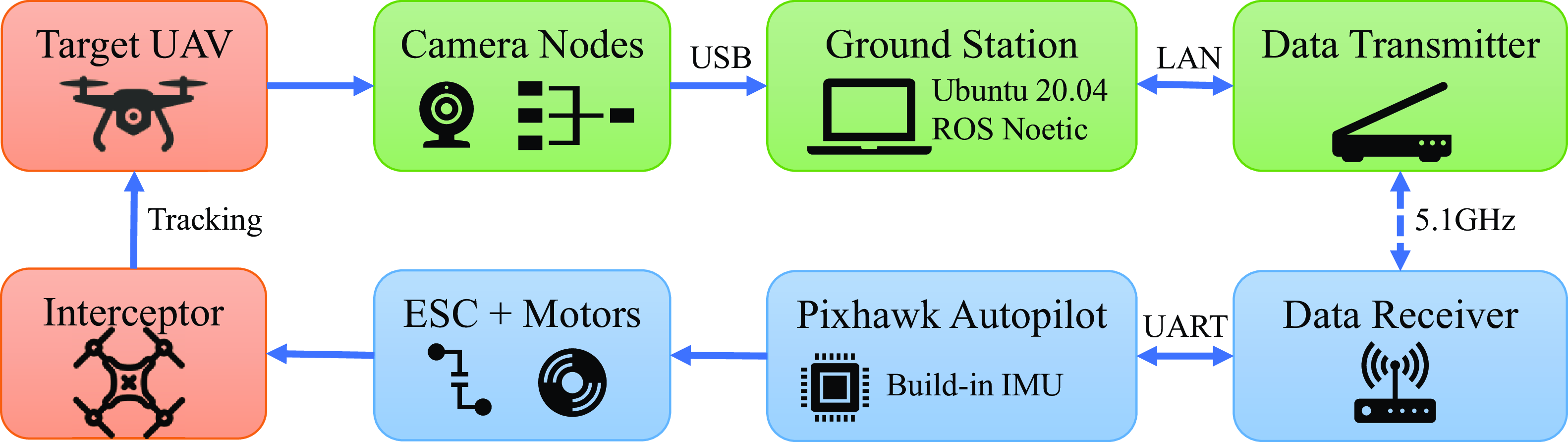
Figure 9 indicates the overall communication structure of the experiment. The camera nodes in the visual sensor network are used to capture video frames of the surveillance area. The video data is transferred via USB to the ground station running Ubuntu 20.04. The visual perception algorithm and the camera network-based intercepting controllers are implemented in ROS kinetic. We use the background subtraction algorithm to detect and track the interceptor and target UAV. Then, depending directly on image errors of the camera nodes, we design the hierarchical interception control algorithm generate the desired thrust and torque. The interceptor quadrotor is equipped with an open-source Pixhawk Nora+ autopilot. Using the data transmitter, the ground station communicates with the autopilot through MAVROS. Moreover, in order to minimize the latency, the data transmission frequency is set as 5.1 GHz. The normalized form of the control commands (the thrust and torque) can directly send to autopilot for actuator controls. Finally, the desired motor rotation speed commands are converted into current signals by ESCs to control the motors for intercept maneuver flight.
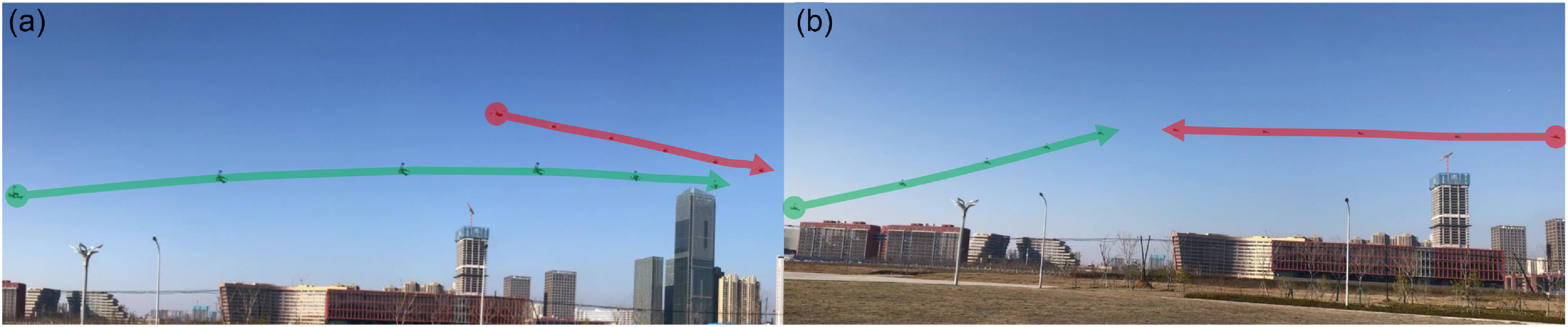
Composite image of (a) tracking and (b) intercepting processes by handheld camera. Snapshots shown every 2.52 s. The filled dots show the positions at the beginning, and the arrows indicate the directions of flights.

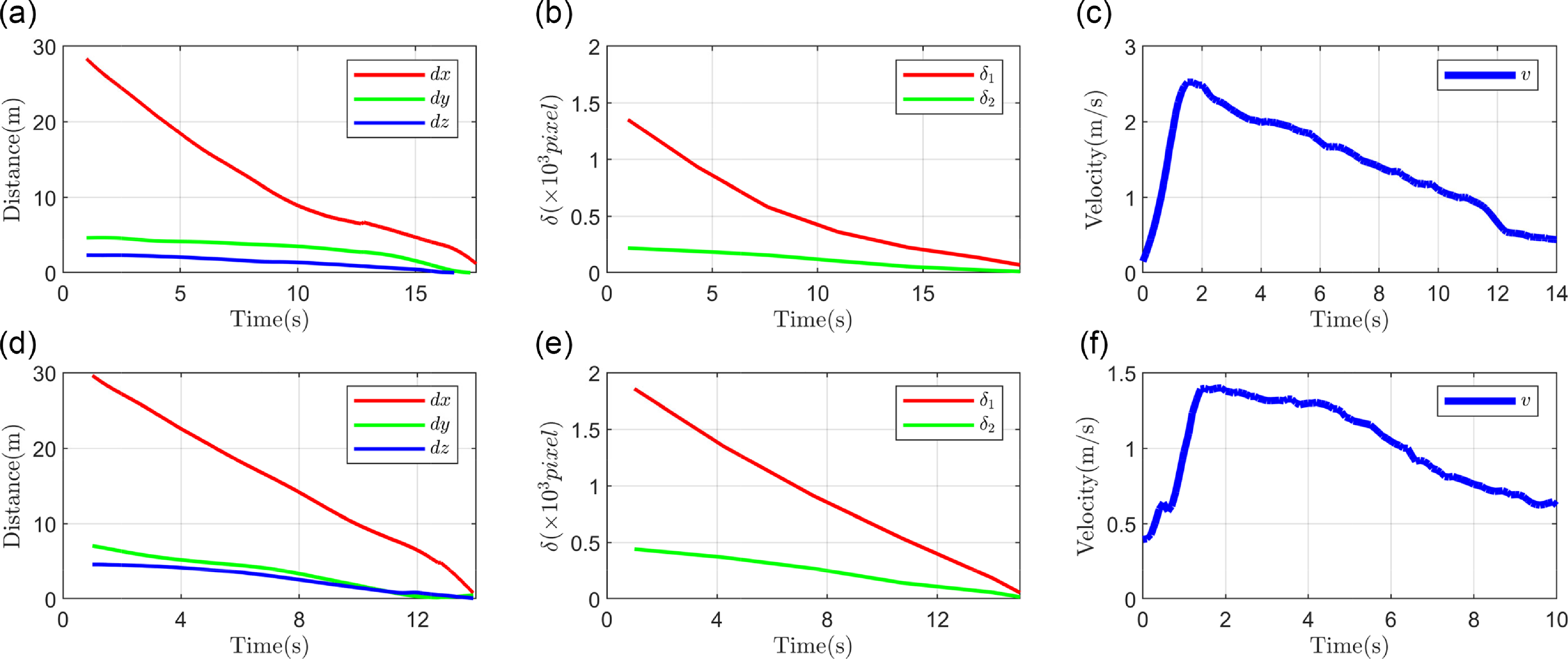
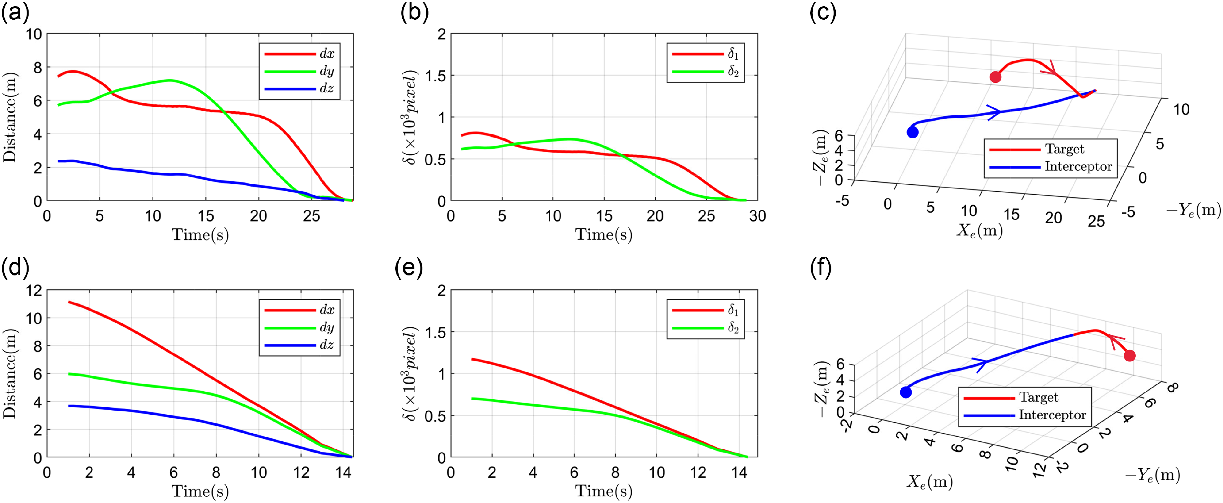
Experiment results: distances between interceptor UAV and aerial target, image error signals of camera nodes and velocities of interceptor UAV. (a), (b), (c) Tracking of a constant-velocity target. (d), (e), (f) Interception of a constant-velocity target.

The trajectories of the two UAVs are presented in Figure 10. It can be seen that the interceptor can track and intercept the aerial target with smooth trajectories. More details can be seen in the video: https://youtu.be/ciewXqvxM84. Figure 11(a), (d) depict the time evolutions of the distances between the interceptor and the constant-velocity target in tracking and intercepting scenarios, respectively. The image error signals from the camera nodes are presented in Figure 11(b) and (e). Also, the linear velocities of the interceptor UAV are shown in Figure 11(c) and (f). In the initial time period (0–1.8 s), the reason for the rapid increase in velocities is the large image errors. As the tracking proceeds, the interceptor gradually approaches the target, the image errors decrease, and the linear velocities decrease accordingly. The results obtained from the varying-velocity target are presented in Figure 12, which fully demonstrate the expected efficacy of the proposed sheme in real environment.
6. Conclusions and future work
In this paper, by utilizing the camera network, a novel eye-to-hand visual servoing approach of UAVs is proposed to address the problem of tracking and intercepting the aerial flight targets. By deriving a visual servoing model to correlate the aircraft motion in the image space and Cartesian space, we designed an IBVS controller directly based on error signals from image planes of the sensor network. The visibility is improved during the interception process, and the stability of the visual servoing system is guaranteed by means of Lyapunov analysis. Moreover, the expected tracking and intercepting performance is proved by experiments in both simulated and real flight scenarios. Compared with classic image-based tracking methods, due to the broad FOV of the camera network, forward interception of the aerial targets is achieved.
Experiment results: distances between interceptor UAV and aerial target, image error signals of camera nodes and flight trajectories. (a), (b), (c) Tracking of a varying-velocity target. (d), (e), (f) Interception of a varying-velocity target. The symbol
 $\bullet$
stand for starting positions.

However, it is impossible for our method to realize the tracking and intercepting under any conditions. When the aerial target is in the blind spot of the camera network’s FOV, or the multiple targets break into the surveillance area at the same time, or the target UAV has stronger maneuverability than the interceptor UAV, the intended interception will not be achieved. In future work, we will focus on optimizing FOV coverage for visual sensor networks, extending our IBVS scheme to multi-intrusion target scenarios and planning more efficient interception trajectories in 3D space.
Author contributions
Guojie Wang and Jiahu Qin conceived and designed the study. Guojie Wang and Qingchen Liu designed experiments and analyzed test data. Qichao Ma conducted theoretical analysis. Guojie Wang wrote the article.
Financial support
This work was supported in part by USTC Research Funds of the Double First-Class Initiative under Grant YD2100002013.
Competing interest
The authors declare no conflicts of interest exist.
Ethical approval
Not applicable.