





1. Introduction
The diffraction of a shock wave into a quiescent medium from a sudden change in area has been studied extensively for decades. Previous work has investigated several features of the problem, including how the shape of the shock wave varies with shock Mach number and wall angle (Skews Reference Skews1967b; Bazhenova, Gvozdeva & Zhilin Reference Bazhenova, Gvozdeva and Zhilin1980), the flow features in the perturbed region behind the shock (Skews Reference Skews1967a; Ishii et al. Reference Ishii, Fujimoto, Hatta and Umeda1999) and how vorticity production varies with wall angle and shock Mach number (Sun & Takayama Reference Sun and Takayama2003; Tseng & Yang Reference Tseng and Yang2006). In addition, a model for the axial decay of a diffracting shock was presented by Sloan & Nettleton (Reference Sloan and Nettleton1975). This model was based on the symmetrical expansion of a so-called critical shock, which is defined as the shape of the shock once the diffraction characteristic arising from the abrupt change in area propagates to the centreline.
The propagation of the diffraction characteristic was studied by Skews (Reference Skews1967b), who experimentally verified Whitham's diffraction theory (Whitham Reference Whitham1957, Reference Whitham1959) and developed an expression for predicting the shock curvature angle  $m_0$. Skews carried out a Huygen's construction for the sound wavefront behind the shock to propagate the disturbance created at the corner of the change in area. Using a simple geometrical argument in the laboratory reference frame (see figure 1), it can be shown that the shock curvature angle
 $m_0$ is related to the initial shock Mach number
 $M_0$ and specific heat ratio of the fluid
 $\gamma$ by
 \begin{equation} \tan^2 (m_0) = \frac{(M_0^2-1)[(\gamma-1)M_0^2+2]}{(\gamma + 1)M_0^4}. \end{equation}
Diagram of the physical shock diffraction problem with the shock curvature angle  $m_0$, initial shock velocity
 $u_0$ and background velocity
 $u_b$ indicated. The diagram indicates the case where
 $u_b = 0$.

This angle defines the locus of the disturbance interaction points along the shock front, as a result of the change in area. In the model of Sloan & Nettleton (Reference Sloan and Nettleton1975), the shock curvature angle is used to determine the critical shock. The expansion of this critical shock was modelled based on the analysis of Chisnell (Reference Chisnell1957) and Sloan & Nettleton (Reference Sloan and Nettleton1975) showed that a shock undergoing symmetrical expansion exhibits a linear relationship between a function derived from the decaying shock strength and the distance from the area change. A similar model was developed for the decay of the wall shock (Sloan & Nettleton Reference Sloan and Nettleton1978).
Skews’ model, which applies to unreactive shock waves, was later extended to detonation waves by Schultz (Reference Schultz2000). Schultz (Reference Schultz2000) applied the Zeldovich–von Neumann–Doring (ZND) one-dimensional model of gaseous detonation (Von Neuman Reference Von Neuman1942; Döring Reference Döring1943; Zeldovich Reference Zeldovich1950), which consists of a strong shock wave and a coupled reaction front propagating at the Chapman–Jouguet velocity (Strehlow Reference Strehlow1968). This expression was then used by Pintgen & Shepherd (Reference Pintgen and Shepherd2009) to investigate the detonation diffraction of two different mixtures in an unconfined half-space. They demonstrated that differences in the failure of the detonation to transition into the unconfined half-space was not due to the differences in the thermodynamic properties of the mixtures. Both Skews’ and Schultz's expressions have appeared in numerous other studies on shock (Sloan & Nettleton Reference Sloan and Nettleton1975; Bazhenova, Gvozdeva & Nettleton Reference Bazhenova, Gvozdeva and Nettleton1984; Thompson, Carofano & Kim Reference Thompson, Carofano and Kim1986; Skews & Kleine Reference Skews and Kleine2009; Ndebele & Skews Reference Ndebele and Skews2019) and detonation (Edwards, Thomas & Nettleton Reference Edwards, Thomas and Nettleton1979; Arienti & Shepherd Reference Arienti and Shepherd2005; Pintgen & Shepherd Reference Pintgen and Shepherd2009; Liang, Mével & Law Reference Liang, Mével and Law2018; Shi, Uy & Wen Reference Shi, Uy and Wen2020) diffraction. In each of these applications, a key assumption remains that there is negligible fluid velocity upstream of the incident shock wave. However, this assumption is not valid in a number of applications.
Several numerical studies have been undertaken on shock diffraction in quiescent media covering a broad range of topics including vortices generated during diffraction (Murugan et al. Reference Murugan, De, Dora and Das2012; Reeves & Skews Reference Reeves and Skews2012; Dora et al. Reference Dora, Murugan, De and Das2014), turbulent structures (Soni et al. Reference Soni, Chaudhuri, Brahmi and Hadjadj2019) and vorticity production (Sivier et al. Reference Sivier, Loth, Baum and Löhner1992; Tseng & Yang Reference Tseng and Yang2006). On numerous occasions, it has been demonstrated that viscous contributions may be neglected and many of the significant flow features associated with shock diffraction are sufficiently captured (Hillier Reference Hillier1991; Sun & Takayama Reference Sun and Takayama1997; Ripley, Lien & Yovanovich Reference Ripley, Lien and Yovanovich2006). Further simplifications to the analysis of shock diffraction include the use of the approximate theory of geometrical shock dynamics (GSD) (Henshaw, Smyth & Schwendeman Reference Henshaw, Smyth and Schwendeman1986). GSD is a nonlinear model for calculating shock motion by propagating the shock along rays normal to the shock front at the local Mach number. As the shock encounters changes in area, the strength of the shock changes.
An analytical model for the change in the strength of a shock wave propagating through a gradually diverging duct was first developed by Chester (Chester Reference Chester1953, Reference Chester1954). This model was developed based on linearised hydrodynamic equations and is only valid for very small changes in area. The model was improved by Chisnell (Reference Chisnell1957), who derived a relationship between the cross-sectional area of the duct and the pressure ratio of the propagating shock wave. Whitham (Reference Whitham1957, Reference Whitham1959) employed the method of characteristics to approach the problem of an expanding shock wave and arrived at a similar relationship to that of Chester and Chisnell. Collectively, the relation they arrived at is known as the CCW relation (Lee & Lee Reference Lee and Lee1965; Zhai et al. Reference Zhai, Liu, Qin, Yang and Luo2010) (acknowledging the contributions of Chester, Chisnell and Whitham). It provides an approximation for the shock motion through changes in area and forms the basis for the theory of GSD. GSD has been used to investigate shock propagation in a wide array of applications including to examine shock wave focusing (Cates & Sturtevant Reference Cates and Sturtevant1997), shock propagation in channels (Schwendeman Reference Schwendeman1993), shock propagation in condensed phase materials (Lieberthal, Stewart & Hernández Reference Lieberthal, Stewart and Hernández2017), magnetohydrodynamic simulations of fast shocks (Mostert et al. Reference Mostert, Pullin, Samtaney and Wheatley2017) and relativistic shock propagation in astrophysics (Goodman & Macfadyen Reference Goodman and Macfadyen2008).
There are several examples of diffracting shock waves propagating in a non-quiescent medium including in the ignition (Boening et al. Reference Boening, Wheeler, Heath, Koch, Mattick, Breidenthal, Knowlen and Kurosaka2018), fuel injection (Prakash et al. Reference Prakash, Fiévet, Raman, Burr and Yu2020) and exhaust (Bach et al. Reference Bach, Thethy, Edgington-Mitchell, Rezay Haghdoost, Oliver Paschereit, Stathopoulos and Bohon2022) processes in a rotating detonation engine (RDE) and the exhaust of pulse-detonation engines (PDEs). The motivation of this paper is to detail how the non-quiescent medium alters the diffraction of a shock wave exhausting from a pulse-detonation combustor (PDC) (Wolański Reference Wolański2013; Pandey & Debnath Reference Pandey and Debnath2016; Rezay Haghdoost et al. Reference Rezay Haghdoost, Thethy, Edgington-Mitchell, Habicht, Vinkeloe, Djordjevic, Paschereit and Oberleithner2021). Rezay Haghdoost et al. (Reference Rezay Haghdoost, Edgington-Mitchell, Paschereit and Oberleithner2020b) demonstrated that the exhaust of the PDC contained either a detonation wave or a strong shock wave decoupled from the reaction front, depending on the fill fraction. In their valveless PDC, the air continuously flows through the combustor; when a detonation is initiated, the flow ahead of the detonation is not stagnant and the assumption of negligible fluid velocity upstream of the propagating shock wave is no longer valid. PDCs promise significant improvements in the efficiency of existing gas turbine engines through pressure-gain combustion (Heiser & Pratt Reference Heiser and Pratt2002). Optimising the efficiency gain from a PDE requires careful selection of the exit geometry and the use of a converging nozzle has been demonstrated to produce an overall pressure gain (Glaser et al. Reference Glaser, Rasheed, Dunton and Tangirala2009). However, geometric modification of the PDC exit with a converging nozzle leads to an increase in the fluid velocity upstream of the propagating shock. This reinforces the need to investigate how shock diffraction is altered by a non-quiescent background medium.
In this paper, we present the diffraction of an initially planar shock wave through a non-quiescent flow of significant velocity. Section 2 details the experimental techniques and numerical methods used to investigate this phenomenon. Experimental results from the exhaust flow of a PDC, using high-speed particle image velocimetry (PIV) and schlieren visualisations, provide a physical example of such a flow in § 3. Following this, we employ an Euler numerical scheme in § 4 to investigate a distortion observed in the experiments. In § 5, further analysis is carried out using a modified GSD scheme, which is formulated with a background velocity term to reproduce the distortion effect. Finally, concluding remarks are stated in § 6.
2. Methods
2.1. Experimental set-up
2.1.1. Facility description
Experiments are undertaken on a PDC, depicted in figure 2. The PDC consists of a deflagration-to-detonation (DDT) section followed by an exhaust tube. The DDT section has a diameter of 40 mm whereas the exhaust tube has a diameter of  $D = 30$ mm. All subsequent dimensions are non-dimensionalised using the exhaust tube diameter
 $D$, unless otherwise specified. The length of the DDT section is 22.8
 $D$. The exhaust tube length is 27.5
 $D$ and 29
 $D$ in the schlieren and PIV measurements, respectively. Hydrogen and air are fed at the upstream end of the DDT section and combustion is initiated by a spark plug. The DDT section contains a number of orifice plates to accelerate the flame and initiate DDT (Gray, Paschereit & Moeck Reference Gray, Paschereit and Moeck2015).
Schematic diagram of the PDC (left) and the schlieren (centre) and PIV (right) imaging systems.

The progress of the detonation is tracked along the exhaust tube using a number of pressure transducers and ionisation sensors. Five piezoelectric PCB112A05 pressure transducers are flush-mounted (Thethy et al. Reference Thethy, Kaebe, Honnery, Edgington-Mitchell and Kleine2020) along the length of the exhaust tube to track the progression of the shock front. These transducers are located 27.3 $D$, 24
 $D$, 17.3
 $D$, 10.7
 $D$ and 4.0
 $D$ from the end of the exhaust tube. To track the reaction front, three ionisation probes are flush-mounted on the opposite side of the first, third and fifth pressure transducers. Data from both sensors is acquired at a sampling rate of 1 MHz using a National Instruments MXI-Express DAQ system. More details on the PDC facility are provided by Rezay Haghdoost et al. (Reference Rezay Haghdoost, Edgington-Mitchell, Paschereit and Oberleithner2020b).
The operating conditions of the PDC are carefully controlled to provide reliable and repeatable operating conditions. The PDC operates in a valveless configuration (Matsuoka et al. Reference Matsuoka, Muto, Kasahara, Watanabe, Matsuo and Endo2017) in which air is continuously fed into the PDC. The air pressure is regulated to ensure a fixed mass flow rate of 100 kg h $^{-1}$ is provided. The fill time, which is defined as the hydrogen injection time, is held constant at 45 ms for all experiments. This provides control of the fill fraction of the PDC but results in only part of the exhaust tube being filled with reactive mixture. Accordingly, the fill fraction of the exhaust tube is less than one. Further details on the control of fill fraction and how it affects the dynamic flow evolution is provided by Rezay Haghdoost et al. (Reference Rezay Haghdoost, Edgington-Mitchell, Paschereit and Oberleithner2020b). The air issues out of the PDC exhaust tube as a steady turbulent jet (or non-quiescent background flow) through which the shock wave diffracts. Ignition of the spark plug is initiated at the same instant that the hydrogen valve is closed. Ambient temperature within the laboratory was measured to be
 $T = 288$ K.
2.1.2. Nozzle configurations
Figure 3 represents the two configurations considered in the experiments: a straight nozzle (figure 3a) and a converging nozzle (figure 3b). The straight nozzle consists of no geometric modification to the exhaust tube and thus has an exit diameter of 1 $D$. For the converging nozzle, the exit diameter is decreased to 0.5
 $D$ over a length of 2
 $D$. This represents a convergence angle of 7.1
 $^{\circ}$ and a blockage ratio of 75 %.
(a) Straight and (b) converging nozzle configurations on the PDC.

2.1.3. Schlieren system
A Toepler Z-type schlieren system (Settles Reference Settles2012) is used to undertake schlieren measurements of the PDC exhaust flow. Figure 2 depicts the experimental set-up which contains two parabolic  $f/8$ mirrors with a focal length of 1219 mm and a high-speed LED (Willert, Mitchell & Soria Reference Willert, Mitchell and Soria2012) operating at an exposure time of 1
 $\mathrm {\mu }$s. The images are captured on a Photron SA-Z high-speed camera at a frame rate of 40 kHz. The knife edge is oriented to provide images of the
 $\partial \rho /\partial y$ path-integrated density gradient.
2.1.4. PIV system
Particle images are obtained using a high-speed camera mounted orthogonally to the exit of the PDC, as depicted in figure 2. The tube and the ambient air near the PDC exit are seeded using an air-driven fluidised bed. Two FDX fluidic oscillators (Woszidlo et al. Reference Woszidlo, Ostermann, Nayeri and Paschereit2015; Sieber et al. Reference Sieber, Ostermann, Woszidlo, Oberleithner and Paschereit2016; Bühling et al. Reference Bühling, Strangfeld, Maack and Schweitzer2021) are used to obtain uniform seeding of the ambient air. Illumination of the particles is provided by a Darwin-Duo diode-pumped Nd:YLF laser operating at a frequency of 10 kHz. Timing for the laser and the camera is controlled using an ILA 5150 synchroniser.
A summary of the PIV parameters is provided in table 1. The flow is seeded with titanium dioxide particles (TiO $_2$) with a relaxation time of
 $0.84\,\mathrm {\mu }$s. A laser pulse separation of
 $4\,\mathrm {\mu }$s is employed. An iterative multigrid scheme is used to cross-correlate the image pairs with an initial window size of
 $96 \times 96$ px and a final window size of
 $64 \times 64$ px. The digital resolution for the straight nozzle is 411 and 225 px
 $D^{-1}$ for the converging nozzle. Spurious velocity vectors are detected using a series of outlier detection filters and erroneous vectors are replaced via interpolation with the neighbouring vectors. Mean PIV vector fields are generated by applying a Chauvenet filter with a maximum allowable sample deviation of three. Further details of the PIV system, including a parameter study on the selection of tracer particles, can be found in Rezay Haghdoost et al. (Reference Rezay Haghdoost, Edgington-Mitchell, Paschereit and Oberleithner2020b).
PIV parameters for the PDC.

2.2. Numerical Euler scheme
2.2.1. Description
Numerical simulations are performed using two-dimensional compressible Euler equations with an axisymmetric source term. In their conservative form, the equations are given by
 \begin{equation} \frac{\partial}{\partial t} \begin{pmatrix} \rho \\ \rho u \\ \rho v \\ \rho E \end{pmatrix}+ \frac{\partial}{\partial y} \begin{pmatrix} \rho u \\ \rho u^2 + p \\ \rho uv \\ u(\rho E + p) \end{pmatrix}+ \frac{\partial}{\partial x} \begin{pmatrix} \rho u \\ \rho uv \\ \rho v^2 + p \\ v(\rho E + p) \end{pmatrix} ={-}\frac{1}{y} \begin{pmatrix} \rho u \\ \rho u^2 \\ \rho uv \\ u(\rho E + p) \end{pmatrix}, \end{equation}
where  $\rho$ is the density,
 $p$ is pressure,
 $\boldsymbol {u}$ is the velocity with velocity components
 $\boldsymbol {u} = (u,v)$ and
 $E$ is the total energy. The total energy is defined by
 \begin{equation} E = e + \frac{\|\boldsymbol{u}\|^2}{2}, \end{equation}
with  $e$ representing the internal energy. Equation (2.1) is closed using the caloric perfect gas approximation which is given by
 \begin{equation} p = \rho(\gamma -1)e, \end{equation}
where the ratio of specific heats (or adiabatic index)  $\gamma$ is assumed constant and
 $\gamma = C_p/C_v = 1.4$ (for air). Equations (2.1)–(2.3) are solved using a fully conservative second-order split finite-volume MUSCL scheme (Van Leer Reference Van Leer1984; Toro Reference Toro2013), discretised on a structured grid. The boundary of the simulation is embedded into the structured grid, which may result in irregular cells. To ensure the stability of any small cells that occur, a conservative cut-cell method is used to ensure that no mass flows through the boundary (Klein, Bates & Nikiforakis Reference Klein, Bates and Nikiforakis2009; Gokhale, Nikiforakis & Klein Reference Gokhale, Nikiforakis and Klein2018). Artificial oscillations at discontinuities in the numerical scheme (such as the shock) are prevented by limiting the slopes of the reconstruction step using the van-Leer limiter (see Toro (Reference Toro2013) for further details). This numerical scheme has been presented in a number of previous works (Nadolski et al. Reference Nadolski, Rezay Haghdoost, Gray, Edgington-Mitchell, Oberleithner and Klein2019; Rezay Haghdoost et al. Reference Rezay Haghdoost, Edgington-Mitchell, Nadolski, Klein and Oberleithner2020a, Reference Rezay Haghdoost, Thethy, Nadolski, Seo, Paschereit, Klein, Edgington-Mitchell and Oberleithner2022) and is well validated.
2.2.2. Initialisation and boundary conditions
The simulation domain consists of a two-dimensional domain (hereinafter referred to as the plenum), in which the shock diffracts, attached to a one-dimensional tube. Altering the input conditions at the tube inlet allows for the conditions through which the shock diffracts in the plenum to be changed. The domain and grid for the tube and plenum are illustrated in figure 4, with the inset showing an example of the mesh for a straight nozzle. To simulate the converging nozzle, the outlet tube is modified and the exit diameter is reduced by 50 % over 2 $D$, analogous to the nozzles described in § 2.1.2. The plenum is
 $10D \times 10D$ and the nozzle exit is located
 $3D$ from the boundary between the tube and the plenum. At this boundary, the values calculated in the tube are assigned equally to all the neighbouring cells in the plenum. The length of the inlet tube ensures that the average centreline velocity of the background flow reaches a steady state before the shock is initialised. The plenum size was sufficiently large to ensure that no artificial reflections or spurious waves altered the results.
Example of the simulation grid discretisation and labelled boundary conditions.

The domain is discretised using a structured grid with one-dimensional cells in the tube region and two-dimensional cells in the plenum region (see figure 4). The domain has a total of 2 504 979 cells for the converging nozzle while the straight nozzle domain has 2 512 904 cells. In both simulations, the one-dimensional tube contains 4448 cells, with the remaining cells located in the two-dimensional plenum. A mesh convergence study is undertaken to ensure the results are independent of grid spacing.
The boundary conditions for the domain are also given in figure 4. Reflective boundary conditions are applied along the centreline and tube walls. The entirety of the left wall of the plenum also has a reflective boundary condition applied. This matches the experiment up to at least  $0.4D$ from the nozzle lip but may differ beyond this point. The upper and far walls of the plenum have transmissive boundary conditions applied. The boundary condition at the inlet of the simulation varies, depending on the simulation phase. At the onset of the simulation, an input mass flow rate for air is applied at the inlet of the tube. The air is allowed to flow through the tube and into the plenum section, giving rise to a jet that reaches a steady state and produces a non-quiescent medium. After 10 ms has passed, a Riemann problem is set up 1.7
 $D$ upstream of the nozzle entrance. For the straight nozzle, this point is also the nozzle exit. A shock Mach number is specified and post-shock values are calculated using the Rankine–Hugoniot expressions. The entire flowfield upstream of this location is assigned the post-shock values. The shock is then allowed to propagate and diffract into the plenum, through the previously initiated non-quiescent background flow. Once the Riemann problem begins, the inlet boundary condition, which previously specified the mass flow rate, is set to a transmissive boundary for the remainder of the simulation. The sensitivity of the position at which the Riemann problem is initiated was investigated, with no discernible change to the results.
2.3. Geometrical shock dynamics
2.3.1. Description
Although the compressible Euler simulations will be shown to capture the key features of the phenomenon under consideration, the mechanism can be demonstrated in a clearer fashion with a reduced-order model. Here, this takes the form of a modified GSD formulation. GSD inherently simulates only the propagation of the shock front, eliminating the effect of any other flow structures. The scheme is based on the CCW relation between the change in shock area  $A$ and the shock Mach number
 $M$ which are related by
 \begin{equation} \frac{{\rm d} A}{A} = \frac{-M \lambda(M)\,{\rm d} M}{(M^2-1)}, \end{equation}
where  $\lambda (M)$ is
 \begin{equation} \lambda(M) = \left(1 + \frac{2 (1-\mu^2)}{\mu(\gamma +1)}\right) \left(1 + 2\mu + \frac{1}{M^2}\right), \end{equation}
with the specific heat ratio of the fluid  $\gamma$ and
 \begin{equation} \mu^2 = \frac{(\gamma -1)M^2 + 2}{2\gamma M^2 - (\gamma-1)}. \end{equation}
The integral of (2.4) provides an expression between the local Mach number and the area of the discretised shock front. Whitham (Whitham Reference Whitham1957, Reference Whitham1959) demonstrated this gives
 \begin{equation} A = A_0 \frac{f(M)}{f(M_0)}, \end{equation}
where the initial shock Mach number is  $M_0$ and the initial ray-tube area is
 $A_0$. This expression includes the function
 $f(M)$, which is given by
 \begin{equation} f(M) = \exp \left(-\int \frac{M \lambda(M)}{M^2-1}{\rm d} M\right), \end{equation}
with all the terms as defined earlier. The shock front is discretised on an orthogonal curvilinear coordinate system, as shown in figure 5. Successive positions of the shock are calculated on this system where shock positions are represented by curves, and the normal vectors along which the shock propagates are traced by rays, given by  $\alpha$ and
 $\beta$, respectively. A rectangular coordinate system is described based on the angle of inclination of the rays relative to the
 $x$ axis. Each discretised shock front segment is specified by the local Mach number, with the local propagation ray described by the ray inclination angle
 $\theta$.
Shock positions (solid) and propagation rays (dashes) in the curvilinear coordinate system ( $\alpha,\beta$), adapted from Rezay Haghdoost et al. (Reference Rezay Haghdoost, Thethy, Nadolski, Seo, Paschereit, Klein, Edgington-Mitchell and Oberleithner2022). The relationship between a rectangular coordinate system and the orthogonal curvilinear system is also shown.

2.3.2. Numerical algorithm
The numerical scheme implemented to solve the GSD problem is similar to that implemented by Henshaw et al. (Reference Henshaw, Smyth and Schwendeman1986). The algorithm involves a leap-frog time-marching scheme where the shock front is described by a set of discrete points. At each time step, the shock is propagated along the local normal ray with a speed calculated from the discrete form of (2.7). Additional shock points are added as the shock expands and shock points leave the calculation domain, ensuring a uniform distribution of shock points is maintained.
The scheme is described as follow. In vector form, the relationship between the shock position and velocity is given on a ray by
 \begin{equation} \frac{\partial}{\partial t} \boldsymbol{x}(\beta,t) = a_0 M(\beta,t) \boldsymbol{n}(\beta,t), \end{equation}
where  $\boldsymbol {x} = (x,y)$ represents the shock position and
 $\boldsymbol {n} = (\cos \theta, \sin \theta )$ gives the normal to the shock front. In (2.9),
 $\alpha$ is eliminated and replaced with the time t using
 $\alpha = a_0 t$, where
 $a_0$ is the ambient speed of sound.
The shock front is discretised into  $N$ points which gives a system of nonlinear ordinary differential equations (ODEs) given by
 \begin{equation} \frac{{\rm d}}{{\rm d} t} \boldsymbol{x}_{i}(t) = a_0 M_{i}(t) \boldsymbol{n}_{i}(t), \end{equation}
where  $i = 1,\ldots,N$. The system is numerically integrated using a two-step leap-frog scheme given by
 \begin{equation} x_i(t+{\rm \Delta} t) = x_i(t- {\rm \Delta} t) + 2 a_0 {\rm \Delta} t M_i(t) \boldsymbol{n}_i(t), \end{equation}
with  $t = n {\rm \Delta} t$,
 $n = 0,\ldots,T/{\rm \Delta} t$ and
 $i = 1,\ldots,N$. The time step
 ${\rm \Delta} t$ is calculated based on the initial shock Mach number
 $M_0$ and the ambient speed of sound to maintain the Courant–Friedrichs–Lewy (CFL) condition (Courant, Friedrichs & Lewy Reference Courant, Friedrichs and Lewy1928). Time marching is undertaken for a fixed number of time steps (
 $n = 500{\,}000$) or until the streamwise or spanwise extent of the shock reaches predetermined cut off values at either the centreline or wall region, respectively. This scheme is second-order accurate in time and Henshaw et al. (Reference Henshaw, Smyth and Schwendeman1986) states that it adds no numerical dissipation, which is desirable for hyperbolic systems such as (2.9).
At each time step, the local Mach number of the shock is determined from (2.7), which is rearranged to give
 \begin{equation} M_i(t) = f^{{-}1}\left(f(M_i(0) \frac{A_i(t)}{A_i(0)}\right), \end{equation}
where  $i = 1,\ldots,N$ and
 $f^{-1}$ is the inverse function of (2.8). To solve for the Mach number, an approximation for the area of the shock front segment is required. In this work, all the flow cases considered are axisymmetric, with the approximate area
 $A_i(t)$ given by
 \begin{equation} A_i(t) = 1/2 {\rm \pi}\begin{cases} (y_{i+1}+y_i)(s_{i+1}-s_i), & {\rm if}\ i = 1; \\ 2y_i(s_{i+1}-s_{i-1}), & {\rm if}\ i = 2,\ldots,N-1; \\ (y_{i}+y_{i-1})(s_{i}-s_{i-1}), & {\rm if}\ i = N; \end{cases} \end{equation}
where  $s_i(t)$ is the arc length of the shock segment and is given by
 \begin{equation} s_i(t) = \begin{cases} 0, & {\rm if}\ i = 1;\\ s_{i-1}(t) + |x_i(t) - x_{i-1}(t)|, & {\rm if}\ i = 2,\ldots,N. \end{cases} \end{equation}
The approximation for the area is based on a central differencing scheme based about the point  $x_i(t)$, with a one-sided scheme employed at the end points. The final parameter required to solve (2.11) is the normal to the shock front. To find the local normal vector, an interpolated cubic spline is fit to the calculated shock front. At any time
 $t$, the normal vector can then be determined from the smooth curve (
 $\tilde {x}(s),\tilde {y}(s)$) by
 \begin{equation} \boldsymbol{n}_i(t) = \frac{(\tilde{y}^{\prime}(s_i), - \tilde{x}^{\prime}(s_i))}{[(\tilde{x}^{\prime}(s_i))^2 + (\tilde{y}^{\prime}(s_i))^2]^{1/2}}, \end{equation}
where differentiation with respect to  $s$ is indicated by the primes, the cubic spline interpolants are given by
 $\tilde {x}(s)$ and
 $\tilde {y}(s)$ and
 $i = 1,\ldots,N$. The number of shock points is selected to provide sufficient resolution of the shock front, with
 $N = 2001$ in this work. Henshaw et al. (Reference Henshaw, Smyth and Schwendeman1986) provides a rule to ensure adequate resolution of the shock front and this value of
 $N$ satisfies the rule. In spite of this, a grid convergence study is undertaken to ensure the number of shock points are sufficient.
2.3.3. Dealing with non-quiescent flows
The description of the GSD formulation has thus far been identical to that given by Henshaw et al. (Reference Henshaw, Smyth and Schwendeman1986), who investigated shock propagation in quiescent media. This formulation was employed in a previous paper (Rezay Haghdoost et al. Reference Rezay Haghdoost, Thethy, Nadolski, Seo, Paschereit, Klein, Edgington-Mitchell and Oberleithner2022) in which it was validated against both experimental results and Euler simulations. We now extend the description to include a non-quiescent background flow. The reactant jet issuing from the PDC exhaust will be shown in § 3 to exhibit a velocity profile typical of turbulent jets, however for the purpose of developing a predictive model, we assume a top-hat velocity profile for the GSD and theoretical development presented herein, as per figure 6. The application of differing spanwise velocity profiles is discussed in Appendix A. In figure 6(b), the spanwise distribution of the velocity profile is indicated, with the region outside of the background remaining quiescent.
(a) A diagram of the nozzle exit and shock state applied in the modified GSD formulation. The quiescent and non-quiescent media are indicated. (b) An example of the spanwise velocity profile showing the quiescent and non-quiescent regions, taken along the dashed line indicated in (a).

To apply this velocity profile, or any other velocity profile for the background flow, we must return to (2.10) and specify that the shock Mach number varies in both time and position. In the simplified model presented here, where it is assumed that no streamwise velocity variation occurs, the non-quiescent GSD can be formulated as
 \begin{equation} \frac{{\rm d}}{{\rm d} t} \boldsymbol{x}_{i}(t) = a_0 \boldsymbol{M}_{i}(y,t) \boldsymbol{n}_{i}(t), \end{equation}
where the shock Mach number is now a function of spanwise position, as shown in figure 6. To solve this new system of ODEs, we employ the same time-marching two-step leap-frog scheme as (2.11), with the Mach number term  $M_i(t)$ now replaced by
 $M_i(y,t)$. In this formulation, shock velocity for each segment is calculated as the sum of the local shock velocity (determined from the local shock Mach number) and the local background velocity. The background velocity is defined on a grid, and the velocity closest to each shock segment is taken as the local background velocity. The sum of the velocities is then converted to a Mach number based on the ambient speed of sound and applied in (2.11) and (2.12), as described previously for the quiescent backgrounds. The introduction of an artificial interface from the velocity profile does not produce any spurious waves as GSD simulates only the leading shock wave.
Although a top-hat velocity profile is applied in the present work, there are no limitations to further velocity profiles or, indeed, velocity fields being applied to the scheme. All that is required is the appropriate assumption for the variation of  $M_i$ in (2.16).
3. Example of shock diffraction through a non-quiescent medium
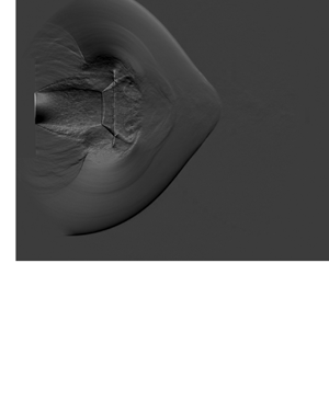
We begin by presenting an example of a physical system in which shock diffraction occurs through a non-quiescent medium. Figure 7 provides sequential schlieren images of a valveless PDC exhaust with a straight (figure 7a,c) or converging (figure 7b,d) nozzle. An initially planar shock propagates down the exhaust tube in the PDC, through the nozzles described in § 2.1.2 and diffracts into the open space beyond. Despite the differences in geometry, figure 7 shows that many of the features behind the leading shock wave remain largely unchanged (Thethy et al. Reference Thethy, Rezay Haghdoost, Oberleithner, Honnery and Edgington-Mitchell2019). The key difference between the two nozzles is in the shape of the diffracting shock wave itself. For the straight nozzle, the angle of the shock wave relative to the  $x$ axis (also referred to as the shock angle
 $\theta _s$, see figure 7b) continuously decreases from
 $\theta _s = {\rm \pi}/2$ at the centreline to
 $\theta _s \approx 0$ in the wall region for the straight nozzle. This is in contrast to the shock angle for the shock wave diffracting from the converging nozzle which, whilst also beginning with
 $\theta _s = {\rm \pi}/2$ at the centreline and ending with
 $\theta _s \approx 0$ at the wall, contains a region of constant shock angle. This is exemplified from around
 $X/D = 0.5$ to
 $X/D = 0.9$ in figure 7(a) and
 $X/D = 1.1$ to
 $X/D = 1.3$ in figure 7(c) and further indicated with red arrows. This feature is henceforth referred to as the spatial distortion of the shock front or the shock distortion.
Two consecutive high-speed schlieren images taken at 40 kHz of the (a,c) straight and (b,d) converging nozzles. The spatial distortion is indicated by the red arrow in both images of the converging nozzle. The definition of shock angle  $\theta _s$ is shown in the inset of (b). Initial shock Mach numbers are (a,c)
 $M_0 = 2.62$ and (b,d)
 $M_0 = 2.41$.

In the exhaust of both nozzles, a background flow is present in the form of a subsonic jet, through which the shock wave diffracts. To investigate the differences in the velocity of the background flow, high-speed PIV of the exhaust flow is undertaken. High-speed PIV from the PDC was reported previously by Rezay Haghdoost et al. (Reference Rezay Haghdoost, Edgington-Mitchell, Paschereit and Oberleithner2020b). From this data, the mean spanwise velocity profile is extracted at a streamwise location of  $X/D = 1$ and presented in figure 8 for both nozzles. The velocity is non-dimensionalised by the ambient speed of sound; all subsequent velocities given in this paper are similarly non-dimensionalised unless otherwise specified. The mean is measured prior to the arrival of the shock from 53 and 55 image pairs for the straight and converging nozzles, respectively. The magnitude of the centreline velocity for the converging nozzle is 2.7 times larger than the centreline velocity for the straight nozzle. Both velocity profiles are typical of turbulent jets and exhibit an inflection point, characteristic of the hyperbolic tangent profile (Michalke Reference Michalke1964). Based on this, the shape of the velocity profile can be modelled using a hyperbolic tangent expression of the form
 \begin{equation} u = a\tanh{(b(y-c))}+a, \end{equation}
where  $a$,
 $b$ and
 $c$ are fitting parameters and
 $y$ is the spanwise location. The results of a least squares nonlinear regression of the form of (3.1) is given in figure 8 for both the straight nozzle (S-FIT) and converging nozzle (C-FIT).
Spanwise velocity profiles of the background flow non-dimensionalised by ambient speed of sound  $a_0$ and measured at a streamwise location of
 $X/D = 1$ for the straight (S) and converging (C) nozzles. Included is both experimental data (EXP) and a least squares regression fit to this data (FIT).

To investigate the origin of the spatial distortion, we measure the velocity of the background flow and the diffracting shock waves. The background velocity is determined based on the regression analysis presented in figure 8 and is given in table 2. The velocity of the shock waves are estimated from schlieren measurements in figure 7. The estimated velocity along the jet centreline is calculated by correlating the position of the undiffracted shock between two subsequent frames and extracting the displacement. To reduce the level of uncertainty in the measurement, schlieren images captured at a frequency of 80 kfps are used to determine the shock velocities. The velocity of the shock is given for both nozzles in table 2. Estimated Mach numbers are provided based on the measured ambient temperature. The uncertainty of the background flow is 1.8 m s $^{-1}$ and is calculated from the particle diameter (Raffel et al. Reference Raffel, Willert, Scarano, Kähler, Wereley and Kompenhans2018) and a subpixel error of 0.1 pixels. The uncertainty of the shock velocity is calculated by conservatively propagating the measurement uncertainty from the camera timing and shock displacement.
Summary of the measured background and shock velocities along with estimated Mach numbers.

In table 2, the initial shock Mach number for both nozzles is similar, with the Mach number of the straight nozzle being marginally higher at  $M_0 = 2.62$ compared with
 $M_0 = 2.41$. In the PDC, the detonation wave propagates until the interface between the air and detonatable mixture, which is determined from the fill fraction of the tube. At this point, the shock wave decouples from the combustion front and the strength of the shock rapidly decays as it propagates, due to viscous effects as well as the Taylor expansion waves behind the detonation (Peace & Lu Reference Peace and Lu2018). The inclusion of a converging nozzle also introduces a significant blockage ratio (75 %) and results in a lower fill fraction from the increased back pressure. This is observed in the time-of-flight measurements of shock speed from the pressure transducers in the exhaust tube, where the shock Mach number increases as the fill time is increased (Thethy et al. Reference Thethy, Rezay Haghdoost, Oberleithner, Honnery and Edgington-Mitchell2019). Inside the converging nozzle, the shock accelerates as a result of shock focusing (Cates & Sturtevant Reference Cates and Sturtevant1997). The result is that there are two competing mechanisms: the decrease in shock velocity due to the reduced fill fraction in the tube and the acceleration of the shock due to shock focusing inside the converging nozzle. These competing mechanisms lead to the similar shock velocities for both nozzles.
In this section, we demonstrated a physical example of shock diffraction through a non-quiescent medium. The result is a distortion of the shock front (figure 7) and it is postulated that the distortion occurs as a result of the significant difference in the velocity of the background medium. This hypothesis is investigated using numerical schemes in the proceeding sections.
4. Isolating the dominant mechanisms of shock distortion
To establish the origin of the shock distortion, the contraction of the nozzle must first be eliminated as a mechanism. It has been previously suggested that shock focusing inside the converging nozzle results in an unequal distribution of shock strength at the nozzle exit and, thus, differing streamwise and spanwise shock propagation velocities (Allgood et al. Reference Allgood, Gutmark, Meyer, Hoke, Katta and Schauer2003; Thethy et al. Reference Thethy, Rezay Haghdoost, Oberleithner, Honnery and Edgington-Mitchell2019). This mechanism is assessed using an Euler scheme with a quiescent medium. Despite the inherent inviscid assumption, Euler schemes have been demonstrated to be reasonable models for shock diffraction from large angle, sharp-edged geometries such as a 90 $^\circ$ corner (Hillier Reference Hillier1991; Rezay Haghdoost et al. Reference Rezay Haghdoost, Edgington-Mitchell, Nadolski, Klein and Oberleithner2020a).
4.1. Quiescent simulation
We begin with a simulation of the converging nozzle where the exit diameter changes from 1 $D$ to 0.5
 $D$ over a converging distance of 2
 $D$, as depicted in figure 3. The background is set to stationary ahead of the shock. A time series of non-dimensionalised velocity contours and the gradient of the normalised density are provided in figure 9. In figure 9(a), the shock propagates into the converging section of the nozzle and experiences a contraction in area. This results in a pseudo-stationary Mach reflection forming, with a Mach stem (A) near the nozzle wall and a triple point (B) between the incident (C) and reflected (D) shock waves.
Time series of Euler numerical simulations of shock diffraction from a converging nozzle into a quiescent medium. Initial flow conditions are  $M_0 = 2.62$ and
 $M_b = 0$. Contours of velocity non-dimensionalised by the ambient speed of sound (a,b) and the gradient of normalised density (c,d) are given in each frame. Flow features are labelled A–K and discussed in § 4.1.

In figure 9(b), evidence for shock focusing inside the nozzle is apparent. The reflected shock wave (E) from the nozzle wall propagates beyond the jet centreline and into the opposite half plane. The Mach stem at the leading shock has grown in size, with the triple point (F) propagating inwards and merging at the jet centreline. This results in another Mach reflection occurring, this time at the centreline. The central shock (G) grows in size and gradually fills out the width of the nozzle, as the shock continues to progress towards the exit. The filled out shock then leads to a Mach stem which propagates towards the jet centreline and repeats the cycle until the shock reaches the exit plane of the nozzle. This process has been investigated previously and described in some detail by Setchell, Storm & Sturtevant (Reference Setchell, Storm and Sturtevant1972).
In the inset to figure 9(b), the velocity of the flow directly behind the shock front is shown in greater detail. The strength of the shock front can be estimated based on the velocity behind the shock which, whilst very similar, varies along the length of the shock front as previously suggested. When the shock reaches the nozzle exit, it undergoes a diffraction process. Expansion waves propagate from the nozzle lip towards the centre of the shock, gradually weakening the shock front. This leads to the shock (H) travelling more rapidly in the streamwise direction than the spanwise direction, as evident in figure 9(c). No shock distortion is observed, with the gradient of the shock front changing uniformly and no region of constant angle between the jet centreline and wall region. Behind the shock, many of the classical features associated with a transient supersonic jet are formed (Thethy et al. Reference Thethy, Rezay Haghdoost, Oberleithner, Honnery and Edgington-Mitchell2019; Rezay Haghdoost et al. Reference Rezay Haghdoost, Edgington-Mitchell, Nadolski, Klein and Oberleithner2020a,Reference Rezay Haghdoost, Edgington-Mitchell, Paschereit and Oberleithnerb). Inside the nozzle, the reflected shock (I) has propagated back and forth between the inner surfaces and the centreline of the nozzle. Due to the supersonic flow behind the incident shock wave, the reflection has not propagated upstream into the tube but remains attached to the point of reflection (J) at the start of the nozzle contraction at  $X/D = -2$.
In the final sequence of the time series, figure 9(d), the primary shock (K) has propagated further from the nozzle exit. Inside the nozzle, the reflected shock (L) has propagated between the nozzle walls a number of times. No distortion is observed in the leading shock front at any point. In figure 7, the distortion was clear after the shock had propagated 1 $D$ from the nozzle exit and was still evident when the shock was 1.5
 $D$ from the nozzle exit. In figure 9, the distortion is not observed at any of these points. Further simulations are undertaken at a range of Mach numbers, including comparable values to that measured in the experiment, and no shock distortion is evident in any quiescent simulations. This suggests that the geometry of the nozzle does not produce the distortion observed in the experiment.
4.2. Non-quiescent simulations
To eliminate the geometric influence of the converging nozzle (which accelerates the background flow), simulations are undertaken with a non-quiescent medium using the straight nozzle. In this section, we present the results of a shock diffracting through background flows with differing magnitudes of velocity from a straight nozzle. By varying the mass flow rate of air at the inlet boundary, the velocity of the background flow at the exit is changed. As discussed previously, the distortion observed in the shock front is postulated to occur as a result of the magnitude of the velocity of the background flow. If this is the case, then a straight nozzle with a significant background velocity would produce the same effect observed in the converging nozzle experiment.
Beginning with a mass flow rate that corresponds to the velocity of the background flow measured by the PIV of the converging nozzle, the inlet boundary condition is set to a mass flow rate of 0.114 kg s $^{-1}$. The shock Mach number is set as 2.62, equivalent to that measured in the straight nozzle experiment. Figure 10 gives a time series sequence with contours of non-dimensionalised velocity and the gradient of normalised density. Most of the flow features are the same as the converging nozzle, with the exception that there is no shock focusing present inside the nozzle. As the shock diffracts out of the nozzle, a small distortion is observed. In figure 10(a), the undiffracted shock (A) and diffracted shock (B) are clearly separated by the point at which the diffraction characteristic meets the shock front (C). In quiescent media, the shock front typically exhibits smooth curvature from this point on (Skews Reference Skews1967b). However, in figure 10(a) we see a rapid decrease in the radius of curvature of the shock when the background flow ends. This discontinuity is aligned with the region where the background flow ends (D), as is seen in the velocity contour in the upper half-plane of figure 10(a). Following the discontinuity, a small distortion in the shock front is observed (E), with a region of constant gradient, similar to that in figure 7.
Time series of Euler numerical simulations of shock diffraction from a straight nozzle with a non-quiescent background medium. Initial flow conditions are  $M_0 = 2.62$ and
 $M_b = 0.38$. Contours of velocity non-dimensionalised by the ambient speed of sound (a,b) and the gradient of normalised density (c,d) are given in each frame. Flow features are labelled A–J and discussed in § 4.2.

In figure 10(b), the expansion characteristic (F) has propagated further along the shock front and the shock distortion is still seen (G). From the velocity contour in the upper half plane, there remains a discontinuous change in the shock curvature, aligned with the boundary of the background jet (H). In figures 10(c) and 10(d), the head of the expansion characteristic has propagated across the shock front and into the opposite half plane. In figure 10(c), the distortion is small but evident near the end of the background flow region ( $Y/D = \pm 0.5$, point I). As the shock propagates further away from the nozzle exit, the level of expansion of the shock increases. In figure 10(d), the boundary between the jet and ambient where the shock distortion was previously identifiable is not immediately obvious, though a small region of constant shock front angle still remains around
 $Y/D = \pm 0.40$ (J). It is expected, over time, the shock front will decay and exhibit spherical decay as the shock strength is more uniform across the front (Sloan & Nettleton Reference Sloan and Nettleton1975). However, the shock has not propagated far enough for the effect of the expansion to outweigh the effect of the background velocity.
The distortion effects demonstrated in figure 10 are relatively weak. To demonstrate a stronger distortion, the velocity of the background flow is now increased by implementing a higher mass flow rate of 0.224 kg s $^{-1}$ at the inlet of the tube. This corresponds to a background Mach number of approximately
 $M_b = 0.75$. The shock Mach number is kept at 2.62, with the time series of velocity contours and gradient of normalised density given in figure 11. Simulations are undertaken at a variety of shock Mach numbers in the vicinity of those measured experimentally, with no significant changes to the results observed.
Time series of Euler numerical simulations of shock diffraction from a straight nozzle with a significant non-quiescent background flow applied. Initial flow conditions are  $M_0 = 2.62$ and
 $M_b = 0.76$. Contours of velocity non-dimensionalised by the ambient speed of sound (a,b) and the gradient of normalised density (c,d) are given in each frame. Flow features are labelled A–O and discussed in § 4.2.

In figure 11(a), the shock (A) has begun the diffraction process, but the head of the expansion characteristic (B) has not propagated far past the boundary of the background jet. In figure 11(b), the shock (C) has now propagated further downstream and interacted with the vortices (D) formed by the Kelvin–Helmholtz (KH) instability in the shear layer of the background jet (Tam & Hu Reference Tam and Hu1989). The interaction of the shock with the vortex distorts the shock front, producing a shock reflection (Inoue & Hattori Reference Inoue and Hattori1999; Edgington-Mitchell Reference Edgington-Mitchell2019). The expansion head (E) has now propagated further along the shock, with the background-induced distortion of the shock occurring between the wall region and the boundary of the jet (F). The shock at the boundary of the jet is undergoing a further local distortion due to the interaction with the vortex. Despite this, a small region of constant shock angle is visible at approximately  $X/D = 0.3$ (F).
In figure 11(c), the leading shock (G) has propagated further from the nozzle, with the expansion head (H) almost approaching the jet centreline and the shock interacting with a number of other KH vortices (I). These interactions, like the initial shock–vortex interaction, have locally distorted the shock front. Despite this, the global spatial distortion that results from the background flow is still evident and begins, as in figure 10, at the boundary of the background flow (J). In figure 7, the shock front did not appear to interact with strong KH vortices as in figure 11. The local distortions due to the shock-vortex interactions make the clear identification of the global background-induced distortion difficult to ascertain.
In figure 11(d), the expansion head has now propagated across the jet centreline and the entirety of the shock front has been diffracted and exhibits a curved shape. The region of the shock within the background jet exhibits continuous curvature between the jet centreline and the boundary of the background jet (K). Outside the background jet, a region of constant shock angle is observed, corresponding to the spatial shock distortion (L). The local distortions due to the interaction of the shock with the KH vortices of the background flow have dissipated, leaving a smooth shock both inside and outside the background flow.
Behind the diffracting shock, the typical flow features associated with a starting or transient jet are formed, with the addition of one flow structure. The interaction of the shock with the first vortex in figure 11(b) produces a shock reflection, which propagates upstream as an acoustic wave ( $X/D = 0.8$ in figure 11(c), point M) (Edgington-Mitchell et al. Reference Edgington-Mitchell, Weightman, Lock, Kirby, Nair, Soria and Honnery2021). This process is described in detail by Inoue & Hattori (Reference Inoue and Hattori1999). The propagation of this sound wave is seen in figure 11(d), where the wave appears to merge (N) with curved barrel shocks (O) that have begun to form the typical Mach disk associated with an underexpanded jet (Edgington-Mitchell, Honnery & Soria Reference Edgington-Mitchell, Honnery and Soria2014).
We have now demonstrated that the geometry does not have an influence on the production of the shock distortion. By maintaining the straight nozzle geometry and simply increasing the magnitude of the background flow velocity, the spatial shock distortion observed in figure 7 is reproduced. Indeed, this demonstrates not only that the previously suggested mechanism of shock focusing does not produce the shock distortion, but that it does not contribute to the observed effect. The effect is independent of the nozzle geometry and a function only of the magnitude of the background flow velocity. The production of KH vortices in the background jet causes further local distortions to the shock front, however the strength of these KH vortices is significantly overestimated by the Euler formulation. To isolate the effect of the mean flow on the shock propagation from the influence of these unsteady structures, in the following section the GSD approach is applied.
5. Non-quiescent shock diffraction using GSD
In § 4, the effects of the geometry and background velocity are decoupled using the Euler simulations, eliminating the contribution of the nozzle as a source of the shock distortion. Instead, the magnitude of the background velocity is suggested as the mechanism responsible for the distortion. In this section, we use a modified GSD scheme to reproduce the distortion effect observed in § 3.
5.1. Modified non-quiescent GSD formulation
To investigate the shock distortion phenomenon, the modified GSD formulation described in § 2.3 is employed. The formulation applies a top-hat velocity profile to the background flow as shown in figure 6, with the top-hat velocity taken as the measured centreline background velocity from table 2. The background jet boundary occurs at  $Y/D = \pm 0.5$ for the straight nozzle and
 $Y/D = \pm 0.25$ for the converging nozzle. In both GSD simulations, a straight nozzle exit is employed along with the shock velocities measured in the experiments (see table 2).
Figure 12 presents a comparison between the experimental schlieren images in figure 7 and a contour of the time-history of shock Mach number from the GSD at two different points in time. The time–history plots represent the calculated local Mach number of the shock segments at various points in time. The GSD is aligned with the experiment based on the position of the shock at the centreline. As mentioned previously, GSD only simulates the shock front and thus is unable to predict the structures behind the shock. The GSD results are generated using a straight nozzle, again reinforcing that the geometry does not govern the shape of the diffracting shock.
Comparison between the experiments and the modified GSD formulation for the converging nozzle (a,b) and straight nozzle (c,d) at two different points in time. The upper half-plane contains experimental schlieren images while the lower half-plane contains the time–history of the shock Mach number. The sketches above the images represent the geometric configuration employed in the experiment and GSD. Key features including the spatial distortion of the shock front (red arrows) and inflection point (I) of the shock are indicated. Initial flow conditions for the GSD are (a,b)  $M_0 = 2.41$ and
 $M_b = 0.38$ and (c,d)
 $M_0 = 2.62$ and
 $M_b = 0.14$.

Excellent agreement is shown between the experiment and the GSD time–history plot for both nozzles. The shock distortion, indicated by a region of constant shock angle, is clearly visible in figures 12(a) and 12(b) and is marked with the red arrows. In figures 12(c) and 12(d), a couple of differences are noted between the experiment and simulation of the straight nozzle. In the experiment, no shock distortion is immediately obvious. However, in the GSD, a small region of constant shock angle is apparent near the boundary of the background jet (also marked with red arrows). This suggests that a shock distortion occurs due to the background flow but it is evidently too small to be visible in the experiment. A second difference is noted at the boundary of the background jet and quiescent ambient, at  $Y/D = -0.5$. In the GSD, a sharp change occurs in the gradient of the shock. This is attributed to the sharp change in the top-hat velocity profile at the lip line.
The fingerprint of the background jet is also visible in the GSD results for both nozzles in figure 12, with a sharp line over which the shock Mach number appears to change. Inside the background jet region ( $Y/D < 0.5$), the shock undergoes the combined effects of wave propagation due to the diffraction of the shock and advection due to additional transport by the background flow. In the region outside the jet (
 $Y/D > 0.5$), the background is assumed to be ambient and the shock only undergoes wave propagation due to diffraction which manifests as the sharp change in shock Mach number.
In the near wall region of both simulations, a small discrepancy is noted between the GSD shape and the experiment. Similar discrepancies have been noted in a number of previous works and are attributed to post-shock effects, which are not modelled in the GSD (Best Reference Best1991; Ridoux et al. Reference Ridoux, Lardjane, Monasse and Coulouvrat2018). This is particularly true for weak shocks, such as the wall shock (Sloan & Nettleton Reference Sloan and Nettleton1978) where the effect of the rapidly expanding flow behind the shock is likely to be of a similar order of magnitude as the diffraction process (Best Reference Best1991). In the present work, the experimental data in figure 12 show an inflection point in the shock front near the wall (labelled point I). This feature is not replicated in any of the GSD simulations and is likely the cause of the discrepancy noted between the experiment and simulation. Despite this, it is remarkable how well the shape of the shock front can be predicted using the simple formulation of the non-quiescent GSD with prior knowledge of only the shock Mach number and the background flow Mach number.
5.2. Predicting the shock curvature angle
It is reasonable to assume that the addition of a background flow will have an effect on some of the flow structures behind the primary shock front. Intuitively, one flow structure that is likely to be affected is the expansion characteristic, previously predicted in non-quiescent flows by (1.1).
To generalise the expression for the shock curvature angle, we examine the construction of the original shock diffraction problem formulated by Skews (Reference Skews1967b). Figure 13 gives a schematic diagram of the geometric relationship between the shock and diffraction characteristic in the laboratorys reference frame. The diagram is drawn assuming a subsonic post-shock flow condition. However, if shock Mach number is sufficient for supersonic post-shock flow, the root of the expansion characteristic will be attached to the nozzle exit and will not propagate upstream into the nozzle. In figure 13(a), the relationship between the shock curvature angle  $m_0$, shock velocity
 $u_0$ and post-shock speed of sound
 $a_1$ is diagrammatically provided. This leads to the geometric expression for
 $m_0$ given in (1.1) and reproduced here
 \begin{equation} {\tan}^2(m_0) = \frac{(M_0^2-1)(\gamma -1)\left(M_0^2 + \dfrac{2}{\gamma -1}\right)}{M_0^4 (\gamma + 1)}, \end{equation}
where  $M_0$ is the initial shock Mach number and
 $\gamma$ is the ratio of specific heats. For clarity, the initial or undiffracted shock Mach number will be subsequently referred to as
 $M_0$ and the local shock Mach number as
 $M_s$. To predict the head of the expansion characteristic in the non-quiescent flow, (5.1) must be reformulated with the background velocity taken into account.
Schematic diagram of the physical shock diffraction problem in the laboratory reference frame along with the geometric relationship between the shock curvature angle  $m_0$, shock velocity
 $u_0$, post-shock velocity
 $u_1$ and post-shock speed of sound
 $a_1$. (a) Original construction of the problem as given by Skews (Reference Skews1967b). (b) Generalised problem with non-quiescent background flow
 $u_b$ ahead of the leading shock.

5.2.1. Generalisation of Skews’ expression
To reformulate (5.1), we first return to figure 13(b) and construct the geometric relationship for  $m_0$, now including an additional term
 $u_b$, which is the velocity of the background flow ahead of the leading shock. From the relationships given, one can construct the expression
 \begin{equation} {\tan}^2(m_0) = \frac{a_1^2-(u_0+u_b-u_1)^2}{(u_0+u_b)^2}, \end{equation}
with all the terms as defined previously and given in figure 13. This expression contains dimensional velocities but it is convenient to introduce a substitution to non-dimensionalise the velocity into Mach number. Thus, we introduce the laboratory-frame shock Mach number  $M_0' = {(u_0 + u_b)}/{a_0}$ and rearrange (5.2) to obtain
 \begin{equation} {\tan}^2(m_0) = \left(\frac{a_1}{u_0+u_b}\right)^2 \left[1 - \left(M_0' \left(\frac{a_0}{a_1} \right) - M_1\right)^2\right], \end{equation}
where  $M_1$ is the post-shock Mach number. The construction of (5.3) has thus far been constrained to the geometric representation of figure 13(b), in the laboratory reference frame. To simplify this expression, we consider instead the shock reference frame: a moving reference frame where the shock is now considered stationary. In the shock reference frame, the relationship for post-shock Mach number is
 \begin{equation} M_1 = \frac{a_0}{a_1} M_0' - M_{y}, \end{equation}
where the Mach number behind the shock is given by  $M_{y} = (u_0+u_b-u_1)/a_1$. For convenience, we introduce the background flow Mach number
 $M_b = u_b/a_0$ and shock reference frame Mach number
 $M_0 = u_0/a_0$. An alternative expression for the Mach number behind the shock, using the Rankine–Hugoniot relations for a moving shock, is
 \begin{equation} M_{y} = \left[\frac{(\gamma-1) (M_0'-M_b )^2+2}{2\gamma (M_0'-M_b )^2-(\gamma-1)}\right]^{1/2}, \end{equation}
where  $\gamma$ is the ratio of specific heats for the gas. To complete the reference frame conversion in (5.4), we require the ratio of the speed of sound across a shock. Again, from the Rankine–Hugoniot relations for a moving shock, we have
 \begin{equation} \frac{a_1}{a_0} = \left[\frac{(M_0'-M_b )^2 (\gamma-1)+2)(\gamma(2(M_0'-M_b )^2-1)+1}{(M_0'-M_b)^2 (\gamma+1)^2}\right]^{1/2}, \end{equation}
which is now in terms of only the laboratory shock Mach number  $M_0'$, the background flow Mach number
 $M_b$ and the ratio of specific heats for the fluid
 $\gamma$. Equations (5.4)–(5.6) can be substituted into (5.3) and simplified to produce
 \begin{equation} {\tan}^2(m_0) = \frac{(\gamma - 1){(M_0'-M_b)}^2 + \frac{2}{(\gamma-1)}}{M_0'^2 (\gamma + 1){(M_0'-M_b)}^2} [{(M_0'-M_b)}^2-1], \end{equation}
which gives a new relationship for the shock curvature angle in non-quiescent background flows. This relationship is built from a geometric argument in the laboratory reference frame and, thus, assumes the the shock Mach number is given in the laboratory reference frame. Practically, it is convenient to recast this expression with the Mach number of the shock in the shock reference frame. Converting between the reference frames gives the new expression for the shock curvature angle
 \begin{equation} {\tan}^2(m_0) = \left(\frac{1}{(M_0 + M_b)^2}\right)\left(\frac{\gamma - 1}{\gamma + 1}\right) \left(\frac{{M_0}^2 + \dfrac{2}{(\gamma-1)}}{{M_0}^2}\right) ({M_0}^2-1), \end{equation}
where we have employed the relation  $M_0' - M_b = M_0$. Equation (5.8) is now the generalised form of (5.1) in the presence of a non-quiescent background flow.
The relationship in (5.8) between the shock curvature angle  $m_0$ in radians, the initial shock Mach number
 $M_0$ and the background flow Mach number
 $M_b$ is plotted as a contour in figure 14. The dashed line reproduces the original expression presented by Skews (Reference Skews1967b). It is clear that in the limit as we approach
 $M_b = 0$, (5.8) collapses to (5.1). As
 $M_b$ is increased, the shock curvature angle is reduced for all shock Mach numbers. The level of reduction of the shock curvature angle is greatest at small
 $M_b$ and displays an asymptotic behaviour as
 $M_b$ is increased.
Shock curvature angle  $m_0$ presented for a range of initial shock Mach numbers
 $M_0$ and background flow Mach number
 $M_b$. The original expression, derived by Skews (Reference Skews1967b), is given as a dashed line.

5.2.2. Verifying the new shock curvature expression
To verify the accuracy of (5.8), we compare the predicted angle with the results from the numerical simulations using both the Euler scheme (figure 15) and the GSD (figure 16). In both figures, the predicted shock curvature angle from (5.8) (dashed white line) and Skews’ original expression in (5.1) (dot-dashed blue line) is presented. Figure 15 illustrates the diffraction of a shock with  $M_0 = 2.62$ into a background flow with
 $M_b = 0.89$ with a contour plot of the magnitude of the gradient of normalised density at one point in time. The location at which the shock curvature begins can be identified through the head of the expansion characteristic, which is clearly visible along the shock front in the contour plot. This characteristic carries the information of the area change across the diffracting shock and separates the undiffracted and diffracted shock components. It is clear that the angle predicted by (5.8) intersects with the shock at the same location as the head of the diffraction characteristic, whereas (5.1) overpredicts the shock curvature angle.


Time-history plots of shock Mach number, computed from GSD, for (a)  $M_0 = 5$ and
 $M_b = 2$ and (b)
 $M_0 = 2.5$ and
 $M_b = 1.0$ with the change in shock angle (
 ${\rm \Delta} m_0 > 0.0014$) indicated in red. Included in both plots is the predicted shock curvature angle based on (5.8) (white, dashed) and from Skews’ original expression (5.1) (blue, dot-dashed).

In figure 16, time–history plots of shock Mach number from the GSD are given for initial shock Mach numbers of  $M_0 = 5.00$ (figure 16a) and
 $M_0 = 2.50$ (figure 16b) with background flow Mach numbers of
 $M_b = 2.00$ (figure 16a) and
 $M_b = 1.00$ (figure 16b). GSD provides no information behind the shock and, thus, to identify the position where the shock curvature begins, we numerically evaluate the gradient of the shock segments inside the background jet (
 $Y/D < 0.5$) and specify that the shock curvature begins where
 ${\rm \Delta} m_0 > 0.0014$. This criterion for
 ${\rm \Delta} m_0$ is the dimensionless equivalent of
 ${\rm \Delta} m_0 > 0.8^{\circ }$, which demonstrates convergence of the calculated shock curvature for a range of different conditions. The points that satisfy this criterion are given by the red line. In figure 16(a), the predicted angle from (5.8) shows very good agreement with the calculated position of shock curvature; the dashed white line lies almost perfectly atop the red line. For conditions below
 $M_0 = 5$, such as
 $M_0 = 2.5$ in figure 16(b), there is a small discrepancy between the calculated shock curvature and the predicted shock curvature angle. This occurs because GSD is based on Whitham's theory (Whitham Reference Whitham1957) and Skews demonstrated (Skews Reference Skews1967b) that at lower Mach numbers, (5.1) has a small discrepancy with Whitham's theory. Nevertheless, the error between the predicted shock curvature and the calculated shock curvature is smaller using (5.8) when compared with (5.1). Figure 16 also shows that (5.8) is a good approximation for low shock Mach numbers and becomes exact for
 $M_0 \geq 5$.
Despite the limitations of the GSD, figure 15 demonstrates that (5.8) is an exact match with the Euler scheme at lower shock Mach numbers. Further tests were conducted for a range of shock and background flow Mach numbers using the Euler scheme, with good agreement found with (5.8) across a range of conditions. It is evident from figures 15 and 16 that the effect of increasing background flow is to delay the arrival of the leading expansion characteristic. With this additional information, we can now return to the shock distortion and discuss the mechanism involved in the production of the distortion.
5.3. Spatial distortion of the diffracting shock front
It has been demonstrated that the background velocity is responsible for the distortion of the shock and this distortion grows as the magnitude of the background velocity is increased. In a quiescent medium, the shock undergoes diffraction; the velocity of the shock is purely dictated by its propagation as a wave. In a non-quiescent medium, the shock will still propagate as a wave. However, the background flow superimposes an additional advection term on segments of the shock (see figure 6). At the boundary between the quiescent and non-quiescent background flow, one part of the shock undergoes additional advection while another does not. The shock front must still remain continuous and, thus, the segment at the boundary is stretched to maintain both conditions. This manifests itself as the shock distortion observed in figure 12. To demonstrate the validity of this mechanism, we develop a model for the weak limit of the shock. The purpose of this model is to investigate whether an increase in the background flow velocity is the physical explanation for why the spatial distortion forms and to remove the dependence on the shock Mach number.
5.3.1. Model for the weak-shock limit
In the weak-shock limit, the shock front is equivalent to an acoustic wave and, thus, cannot be weakened by the diffraction process. The diffraction of an acoustic wave thus differs in that propagation velocity does not vary with angle from the downstream axis, unlike the diffraction of a shock of finite strength. We assume here that the temperature in the quiescent and non-quiescent regions is equal and, thus, the speed of sound is constant throughout the domain. This allows us to consider the propagation of the shock due to wave transport as being constant in both the streamwise and spanwise directions. Inside the background region, the additional transport from the background flow advection can simply be added to the shock speed. This is demonstrated diagrammatically in figure 17.
Model for predicting the shock distortion angle  $m_1$ in the weak-shock limit.

Consider a point in time when the shock has travelled downstream of the nozzle exit to a distance of  $x_b$ at the centreline with a velocity of
 $M_s+M_b$, where
 $M_0 = M_s$ and
 $M_S \to 1$. From figure 14 we know that the shock curvature angle in the weak limit approaches
 $m_0 \to 0$, which suggests that a sufficiently weak shock will remain largely straight between
 $y = 0$ and
 $y = y_0$ in figure 17. To simplify the model, we assume that in the weak limit the shock remains entirely straight in the background flow region. Meanwhile, in the radial direction, the shock travels with velocity
 $M_s$ and diffracts, producing a circular shock (in the axisymmetric plane of figure 17). The circular region produced by the radial shock propagation and the straight region inside the jet boundary are joined by a linear shock, representing the shock distortion with angle
 $m_1$.
To predict  $m_1$, we enforce a set of conditions on the linear shock depicted in figure 17. The linear shock must be tangent to the circular shock in the near-wall region, and must intersect with the straight shock inside the background flow region at the jet boundary. Enforcing these conditions leads to three simultaneous equations, which are
 \begin{gather} (x_i - x_0)^2 + (y_i - y_0)^2 = R^2, \end{gather}
 \begin{gather}\frac{x_i - x_0}{\sqrt{R^2-(x_i-x_0)^2}}=m, \end{gather}
 \begin{gather}y_i = m(x_i-x_b)+y_0. \end{gather}
These three expressions represent the shock distortion model in the weak-shock limit. Equation (5.9) yields a circle with a radius  $R$ based on the velocity
 $M_s$ centred at the lip of the nozzle exit (
 $x_0,y_0$) to model the circular shock. The gradient
 $m$ of the tangent of this circle at the intersection (
 $x_i,y_i$) of the circular and linear shock regions is specified in (5.10). Finally, the expression for a straight line between (
 $x_i,y_i$) and the point at the jet boundary (
 $x_b,y_0$) is given in (5.11). Solving these expressions leads to the following analytical relation for the gradient
 $m$
 \begin{equation} m ={-} \frac{R}{\sqrt{x_b^2 - R^2}}, \end{equation}
where  $R$ and
 $x_b$ are defined in figure 17. Substituting the appropriate quantities based on assumptions of the streamwise and spanwise velocity of the shock yields
 \begin{equation} m_1 = \tan^{{-}1} \left(-\frac{M_0}{\sqrt{2 M_0 M_b + M_b^2}}\right), \end{equation}
with the angle  $m_1$ of the shock distortion (in radians) presented as a function of only the shock Mach number
 $M_0$ and background flow Mach number
 $M_b$.
Due to limitations in the operating parameters of the experimental facility and the overprediction of the strength of the KH vortices in the Euler scheme, we employ numerical results from the GSD to verify the predictions from (5.13). However, in figure 16, we acknowledged that there are well-established limitations of GSD for  $M_0 < 5$. Thus, to verify the suitability of the GSD for the forthcoming comparisons, we compare the predicted shock distortion angles
 $m_1$ from GSD with the limited number of available experiments. We find that the average discrepancy between the experimental value and numerical prediction for the available data is
 $2.5^{\circ }$ with a maximum discrepancy of
 $5^{\circ }$. Further details on the comparison between the GSD and experiments are given in Appendix B.
Figure 18 presents a comparison between the results predicted by (5.13) and numerical results from the GSD for a range of conditions. To represent the weak-shock limit, the GSD is undertaken with an initial shock Mach number of  $M_0 = 1.001$. The shock distortion angle
 $m_1$ is measured for each simulation at
 $X/D = 0.8$ and
 $Y/D = 0.55$, which ensures the straight shock region has formed in all the cases tested. To confirm the shock distortion angle was independent of the measurement location,
 $m_1$ was also measured at
 $X/D = 0.2$,
 $Y/D = 0.55$ with no discernible difference found with the values in figure 18. The model shows very good agreement in the weak-shock limit for a broad range of conditions from
 $M_b = 0.05$ to
 $M_b = 3$. The discrepancy between the model and the weak-shock limit results at high
 $M_b$ is due to the shock curvature angle
 $m_0$, which is non-zero for
 $M_0 = 1.001$. As the shock Mach number is increased, the model begins to either under or over predict the shock distortion angle. This is to be expected, as the model is based on the assumption that the propagation velocity is invariant with angle, which is only true in the weak limit. This and other nonlinear effects, such as a change in the shock curvature angle
 $m_0$ (see figure 14) and the formation of a wall shock (Sloan & Nettleton Reference Sloan and Nettleton1978), lead to deviations from the assumptions in figure 17. These are discussed further in the next section. Despite the limitations of GSD at low Mach numbers, figure 16 demonstrates that the discrepancy between the GSD and the available experimental results is not greater than that between the weak-shock limit model and the GSD.
Comparison between the model for the shock distortion angle  $m_1$, measured in radians and predicted by (5.13), and the measured values from GSD simulations for a number of initial shock Mach numbers
 $M_0$ and background flow Mach numbers
 $M_b$.

5.3.2. Nonlinear effects
We see in figure 18 that increasing the shock Mach number leads to a discrepancy between the predictions from (5.13) and the measured angles for  $m_1$ from the GSD. There are a number of nonlinear effects that occur as the shock Mach number is increased that lead to this discrepancy. First, as noted previously, the weak-shock limit model assumes that the shock Mach number is equal in the streamwise and spanwise directions. Further, as
 $M_0$ is increased, for geometry that includes a wall perpendicular to the downstream axis, a wall shock forms in the region where the shock impinges upon this wall. This wall shock is a complex phenomenon and while typically normal to the wall and tangent to the main shock curve, the wall shock can also be curved along the entire length or contain a point of inflection (Skews Reference Skews1967b). Skews (Reference Skews1967b) also showed that the velocity of the wall shock is also known to vary greatly as the shock Mach number is increased, which further violates the assumption that the streamwise and spanwise shock propagation velocities are equal. The second nonlinear effect is the change in the shock curvature angle
 $m_0$. As
 $M_0$ is increased, the assumption that
 $m_0 \to 0$ is no longer valid (see figure 14). As
 $M_0$ is increased,
 $m_0$ grows and increases the disparity with the modelled straight shock inside the background flow region. A third effect that is not considered in the shock distortion model is the change in the shock Mach number as the shock diffraction process occurs. In the weak limit, the shock propagation velocity is constant but as the shock Mach number is increased and the diffraction process takes place, the velocity of the diffracted shock will vary from that of the undiffracted shock.
These nonlinear effects produce competing mechanisms that seek to increase and decrease the shock distortion angle. These effects also help explain the underprediction and overprediction in figure 18. To demonstrate this more clearly, we present two example cases from the GSD result in figure 19. Figure 19(a) displays  $M_0 = 1.5$ and
 $M_b = 0.05$ while figure 19(b) shows
 $M_0 = 5.0$ and
 $M_b = 2.0$ which underpredict and overpredict
 $m_1$ in figure 18, respectively. The solid line represents the calculated shock shape from the GSD at one point in time whereas the dashed and dotted quarter arc, dashed straight line and dotted straight line represent the circular wall shock, the straight shock inside the background flow region and the linear shock modelling the distortion. The GSD result is given at a single point in time and the predicted shapes are based on the model in figure 17 (5.9)–(5.11). Although the jet shock and circular shock are updated for the current shock position, the linear shock is modelled from (5.13) and is thus fixed.


In figure 19(a), it is apparent that the shock distortion angle is underpredicted, with the gradient of the shock segment at the jet boundary ( $Y/D = 0.5$) being greater than the gradient of the linear shock. As the shock Mach number is increased, the shock curvature angle also increases and deviates from the assumption of a straight shock in the background flow region (labelled as the jet shock in figure 19). A normal wall shock is also formed, which propagates at a lower velocity and makes the circular shock assumption in the near-wall region a poor approximation. The combined effect leads to the underprediction of the shock distortion angle. In contrast, figure 19(b) shows that the shock distortion angle is now overpredicted, with the gradient of the shock segment at the boundary being smaller than the gradient of the linear shock. The increased shock Mach number (
 $M_0 = 3.0$) increases the size of the normal wall shock, further violating the circular shock approximation at the wall. The relative propagation velocity of the wall shock propagation is significantly slower than the jet shock (Skews Reference Skews1967b), violating another assumption in the weak-shock model and significantly decreasing the shock distortion angle. The circular component of the shock front is now closer to the shock at the boundary, which would increase in the shock distortion angle. Along with this, the greater
 $M_0$ means the shock curvature angle has increased and there is a greater deviation from the assumed straight jet shock shape. The combined effect of these deviations leads to the overprediction of the shock distortion angle.
Whilst producing a simple model for the shock distortion angle is challenging when the shock Mach number increases beyond the weak limit, we can provide a qualitative description of the change in the shock distortion angle with both shock Mach number and background flow Mach number. For a fixed shock Mach number, the increase in the background flow Mach number leads to a decrease in the shock distortion angle. This is evident from figure 18. In the model presented in figure 17, the point of contact between the circular and linear shocks moves closer to the wall as a result of the changing shock distortion angle and the requirement for the linear shock to be tangent to the circular shock. When the shock Mach number is increased, the wall shock length and angle both grow. This introduces a further normal wall shock to the model in figure 17, however we must acknowledge the earlier shortcomings of predicting the wall shock using GSD and caution that the dynamics of the wall-shock region are likely to be significantly more complicated. This makes development of a simple model to predict the distortion angle challenging. The purpose of the weak-shock limit model is not to act as a predictive tool but rather provide an explanation for why the spatial distortion forms. Despite the significant shortfalls of the simple model, it provides a good description of the physics and is able to capture all the trends in the data which suggests that the proposed mechanism is valid. Furthermore, the predicted shock distortion angles still fall remarkably close to those measured in the GSD up to  $M_0 = 2$. As
 $M_0$ is increased beyond this, the disparity between the predicted and actual shock distortion angles increases.
5.4. Axial decay of diffracting shock
The final feature of the non-quiescent shock diffraction problem that is investigated is the axial (or streamwise) decay of the shock at the jet centreline. Intuitively, we expect there to be a change in the axial propagation of the shock due to both the change in the shock curvature angle and the further advection of the shock by the background flow. To investigate this, we examine the centreline shock Mach number using GSD for various background flow Mach numbers and a fixed initial shock Mach number. This is presented in figure 20 for an exemplar shock Mach number of  $M_0 = 5$. Figure 20 shows that the shock Mach number is initially constant for a period of time before rapidly decaying. For
 $M_b = 0$, the decay is consistent with asymptotic theory of blast waves, producing an exponent of 0.42 which is close to the expected exponent of 0.40 for classical spherical wave decay (Edwards et al. Reference Edwards, MacKinnon, Zweiback, Shigemori, Ryutov, Rubenchik, Keilty, Liang, Remington and Ditmire2001; Zel'Dovich & Raizer Reference Zel'Dovich and Raizer2002). As
 $M_b$ is increased, the shock is advected further away from the nozzle exit and the arrival of the expansion characteristic at the centreline is delayed. This leads to the decay in the shock Mach number beginning later and the shock curvature angle decreasing, which is consistent with (5.8) and figure 14. For
 $M_b \neq 0$, the exponent from the asymptotic theory of blast waves for the decay curve increases as
 $M_b$ increases. At
 $M_b = 0.25$, the exponent is already 0.66 which indicates that the shock no longer exhibits spherical wave decay but rather a more complex decay pattern. However, once the shock begins to decay, the increase in background velocity leads to an apparent increase in the rate of decay of the shock Mach number. This is indicated by all cases with
 $M_b > 0$ crossing the line for
 $M_b = 0$ in figure 20. This trend is repeated across several different initial shock Mach numbers and is not isolated to the specific case shown in figure 20. An explanation of the behaviour of the shock as
 $M_b$ is increased is the subject of this section.
Centreline shock Mach number  $M_s$ (shock reference frame) as a function of axial position for an initial shock Mach number
 $M_0 = 5$ and various background flow Mach numbers
 $M_b$.

Understanding the behaviour of the shock requires further examination of the derivatives of the shock Mach number. The derivative of the shock Mach number with respect to position in the laboratory reference frame is presented in figure 21(a). We observe that the delay in the arrival of the diffraction characteristic, as  $M_b$ increases, is captured in the derivative of
 $M_s$. Once the expansion arrives and the decay of
 $M_s$ begins, the rate of decay is found to be the greatest for the case where
 $M_b = 0$ and gradually decreases as
 $M_b$ is increased. While shock propagation is measured in the laboratory reference frame, it is difficult to elicit meaning from quantities in two different reference frames. If we instead examine the position of the shock in the shock reference frame, we may be able to reconcile the behaviour of the shock in figure 20. The relationship between the shock position in the laboratory reference frame
 $X$ and the shock position in the shock reference frame
 $X_s$ is described at any point in time
 $t$ by
 \begin{equation} X(t) = X_s(t) + a_0 M_b t, \end{equation}
where  $a_0$ is the ambient speed of sound and
 $M_b$ is the background flow Mach number. The derivative of
 $M_s$ with respect to position in the shock reference frame is given in figure 21(b). The trend observed previously is now reversed and we see that as
 $M_b$ is increased, the rate of decay remains very similar. However, the absolute magnitude of the maximum rate of decay increases as
 $M_b$ is increased, suggesting that a greater background flow will lead to a greater decay in the centreline shock Mach number. This is now in accordance with the result given in figure 20.
Derivatives of the shock Mach number  $M_S$ with respect to shock position in the shock
 $X_S$ and lab
 $X$ reference frames for an initial shock Mach number
 $M_0 = 5$ and various background flow Mach numbers
 $M_b$.

To further investigate the trends in figures 21(a) and 21(b), the second derivative of the shock Mach number is given with respect to position in the laboratory (figure 21c) and shock reference frames (figure 21d). It is apparent that in figure 21(c), the gradient of each curve in figure 21(a) changes by differing amounts as  $M_b$ is increased. Furthermore, the magnitude of the maximum rate of decay of the curves decreases as
 $M_b$ is increased. However, as expected, the trend is reversed in figure 21(d) where the magnitude of the maximum rate of decay of the curves in figure 21(b) marginally increases as
 $M_b$ is increased.
The arrival of the expansion head leads to the start of the decay in shock Mach number in figure 20 and this is captured in figure 21. This decay continues until the arrival of the expansion tail, at which point the rate of decay of shock Mach number reduces. In figure 21(b), this is marked by the trough of each curve. The position of the trough translates further downstream as  $M_b$ is increased and the magnitude of the gradient of the shock Mach number also increases as
 $M_b$ is increased. The mechanism that causes the delay of the expansion head is the additional transport of the shock front due to advection by the background flow. The behaviour seen in figure 21(b) is attributed to the same mechanism, which would also be acting on the expansion tail. As the initial Mach number of the shock is held constant, the strength of the expansion should be the same for each
 $M_b$. If we return to figure 21(d), we see that the shape of each curve follows a very similar profile, suggesting the gradient of the curves in figure 21(b) may be collapsed with appropriate scaling.
If the second derivatives of the shock Mach number in figure 21(d) are scaled by a common factor, then the application of an appropriate scaling factor will collapse them all into a single curve. A theoretical scaling factor is developed from the decay mechanism. We know that the diffracted and undiffracted shocks are separated by the arrival of the head of the expansion characteristic. Once the expansion arrives, the pressure behind the shock front reduces, weakening the strength of the shock. In § 5.2, the shock curvature angle, defining the locus of points along the shock front that separates the diffracted and undiffracted shock fronts, is generalised. Accordingly, the shock curvature angle defined in (5.8) can be used to estimate the arrival of the expansion characteristic at the centreline for  $M_b = 0$ and
 $M_b \neq 0$. The difference in the estimated arrival position of the expansion for
 $M_b = 0$ and
 $M_b \neq 0$ is given by
 $X_b$ which is calculated from
 \begin{equation} X_b = \frac{D}{2} \cot(m_{0,b}) - \frac{D}{2} \cot(m_{0,0}), \end{equation}
where  $D$ is the nozzle diameter,
 $m_{0,0}$ is the shock curvature angle for
 $M_b = 0$ and
 $m_{0,b}$ is the shock curvature angle for all
 $M_b$. To demonstrate that the curves in figure 21(d) collapse,
 $X_b$ can be subtracted from the position of the curves.
The result of scaling the curves in figure 21(d) using (5.15) is given in figure 22. The curves collapse with a small discrepancy noted, which increases as  $M_b$ is increased. This occurs as the shock curvature angle overpredicts the arrival of the expansion head at the centreline due to the Mach reflection (from the requirement that the shock is normal at the centreline). This is exemplified in figure 16(a). It is remarkable that each of the curves follow such similar trends and suggests that the underlying mechanism underpinning the axial decay of the centreline shock Mach number is the same for all
 $M_b$. Sloan & Nettleton (Reference Sloan and Nettleton1975) previously suggested that the arrival of the expansion head marked the formation of the critical shock, which after some time would become a spherically expanding shock. The result in figure 22 implies that the transition from the critical shock to the spherically expanding shock occurs very quickly and that the background flow does not affect the spherical expansion of the shock at the centreline significantly.
Second derivative of centreline shock Mach number  $M_s$ with respect to position (in the shock reference frame
 $X_s$) as a function of axial lab reference frame shock position
 $X$ for an initial shock Mach number
 $M_0 = 5$ and various background flow Mach numbers
 $M_b$. Curves are identical to those presented in figure 21(d), with the exception that they are scaled using (5.15).

In figures 21(a) and 21(b), an inflection point is observed in the gradient of the shock Mach number for the cases when  $M_b \neq 0$, before returning to the same trend observed for
 $M_b = 0$. The inflection point travels downstream as
 $M_b$ is increased and the rate of increase in the decay of the shock, after the inflection, is greatest at low
 $M_b$. Sloan & Nettleton (Reference Sloan and Nettleton1975) noted that their model for spherical decay was valid only until approximately
 $X/D = 4$ and the present results support that, with the deviation and formation of these unexpected inflections occurring after approximately
 $X/D = 3$ and the validity of the model in question beyond that.
Finally, further evidence is provided of the arrival of the expansion fan at the centreline through the gradient of normalised pressure from the Euler simulations in figure 23. The arrival of the head of the expansion fan is clearly seen in figure 23(a) (and marked with a blue arrow). The arrow also marks the direction of propagation of the expansion. The arrival of the tail is more complex and not as easily identifiable. To demonstrate that the expansion tail has indeed arrived, we instead examine the sequence in figures 23(a)–23(d), looking at the centreline region near the shock. In figure 23(b), the expansion has yet to arrive which is indicated by the lack of curvature of the shock and negligible pressure gradient immediately behind the shock at the centreline (see point A in the inset). In figure 23(c), the expansion head arrived and a large pressure gradient is seen behind the shock at the centreline (B), indicating the shock is undergoing a decay. In figure 23(d), the expansion tail has arrived and the decay of the pressure behind the shock front from the expansion has ceased (C). We see that the root of the shock is at approximately  $X/D = 1.7$ and from figure 21, it is expected that both the head and tail of the expansion have arrived at the centreline by this point.
Pressure contour from the Euler simulation, also presented in figure 11, showing the arrival of the expansion at the centreline. The head of the expansion fan is clearly seen and is indicated by the blue arrow in figure 23(a). Flow features are labelled A–C and discussed in § 5.4. Initial flow conditions are  $M_0 = 2.62$ and
 $M_b = 0.76$.

To summarise the axial decay behaviour, the current findings suggest that the inclusion of a background flow leads to an increased rate of decay for the axial shock Mach number (see figure 20). Figure 21 suggests that the arrival of both the head and the tail of the expansion fan at the jet centreline are delayed by the advection of the shock by the background flow. Whilst the strength of the expansion remains constant (due to the fixed initial shock Mach number), the delay in the expansion leads to an increase in the magnitude of the gradient of shock Mach number. Despite changing  $M_b$, the axial shock decay scales with the position of the expansion head at the centreline and suggests that the decay mechanism is independent of
 $M_b$ until at least
 $X/D = 3$. This also suggests that the spherical decay model presented by Sloan & Nettleton (Reference Sloan and Nettleton1975) remains valid for increasing
 $M_b$.
6. Conclusions
In this work, an investigation has been carried out on the diffraction of shock waves through a non-quiescent medium. The diffraction of a shock wave generated by a valveless PDC has been presented as a physical example of this process, with high-speed schlieren and high-speed PIV measurements undertaken of the PDC exhaust with a straight and converging nozzle. A time series of the schlieren indicates that the shock front diffracting from the converging nozzle is distorted, with a region of constant shock angle present between the centreline and the wall region. This distortion does not appear to be present in the straight nozzle. Upon examination of the mean spanwise velocity profile of the background flow ahead of the shock, a significant difference has been noted in the velocity of the flow ahead of the converging nozzle; the converging nozzle accelerates the velocity of the background by a factor of 2.7 compared with the straight nozzle.
The mechanism that drives the shock distortion has then been investigated using two numerical schemes. First, an Euler scheme was used to eliminate the geometric influence of the nozzle on the shock diffraction. Using this scheme, simulations have been carried out for a converging nozzle with a quiescent background, demonstrating that no shock distortion occurs. Further simulations have been undertaken with a straight nozzle and a non-quiescent background flow of two different velocities. We have demonstrated that the inclusion of the background flow ahead of the shock leads to the distortion seen in the experiment and by simply increasing the magnitude of the background flow velocity, we have been able to recreate the shock distortion using a straight nozzle exit geometry. However, the strength of the KH vortices in the background flow are significantly overpredicted by the Euler computations and the resulting shock-vortex interaction leads to a further distortion of the shock front.
With the geometric influence of the nozzles excluded, the shock distortion has been investigated using a modified GSD numerical scheme, which includes the background flow. The scheme has been verified against the experimental results and shows remarkable agreement, with the GSD requiring an input of only the shock Mach number, background flow velocity and gas properties. This scheme has then been used to investigate the spatial distortion further, including providing a qualitative description of how the distortion changes with increasing shock and background flow velocities. It has been found that the inclusion of background flow leads to a delay in the head and tail of the expansion characteristic. A new expression has been introduced for the arrival of the head of this expansion, generalising a previous result given by Skews (Reference Skews1967b). A simple model has been developed to predict the shock distortion angle in the weak-shock limit and verified against computations for a range of conditions with the GSD. Finally, the axial decay behaviour of the shock has been investigated and it has been found that increasing the background flow leads to an increase in the decay rate of the centreline shock Mach number. This behaviour was explained using the derivatives of the shock Mach number with respect to position in both the shock and lab reference frames and linked to changes in the behaviour of both the head and tail of the expansion characteristic.
Funding
The authors gratefully acknowledge the support of the Deutsche Forschungsgemeinschaft (DFG) as a part of collaborative research centre SFB 1029 ‘Substantial efficiency increase in gas turbines through direct use of coupled unsteady combustion and flow dynamics’ in Project C01. The authors also acknowledge financial support from the Australian Research Council through discovery project DP190102220. This research is supported by an Australian Government Research Training Program (RTP) Scholarship and by a German Academic Exchange Service (DAAD) Fellowship.
Declaration of interests
The authors report no conflict of interest.
Appendix A. Application of differing spanwise background velocity profiles in the GSD
The modified GSD formulation presented in § 2.3 employs a top-hat velocity profile for the background flow. The motivation for the top-hat profile as opposed to a hyperbolic tangent, which would match the experimental PIV results in figure 8, is a desire to conduct a direct comparison between the GSD results and a simple model for the shock distortion angle (see § 5.3). This appendix demonstrates how the application of a hyperbolic tangent profile changes the GSD results.
Figure 24 illustrates an example of the top-hat and hyperbolic tangent spanwise velocity profiles for a background flow of  $M_b = 0.38$. The top-hat profile is described in § 2.3.3. The hyperbolic tangent profile maintains the same average velocity across the span of the jet. The gradient of the profile at the boundary between the background flow and quiescent media in the experiment is unknown since the spanwise velocity profile is not available at the nozzle exit. Thus, an arbitrary constant that reduced the sharp velocity transition at the boundary between the background flow and quiescent media was selected.
Example of the top-hat and hyperbolic tangent spanwise velocity profiles for a background flow of  $M_b = 0.38$.

A comparison between the experimental results and the modified GSD using both a top-hat and hyperbolic tangent velocity profile is given in figure 25. Figure 25(a) presents the propagation of a  $M_0 = 2.62$ shock through a background flow of
 $M_b = 0.38$ while figure 25(b) presents the propagation of a
 $M_0 = 2.41$ shock through a background flow of
 $M_b = 0.14$. In both figures 25(a) and 25(b), the top-hat and hyperbolic tangent velocity profiles match the experimental results for inside the background flow. Outside the background flow, the top-hat profile predicts a shock distortion angle that is closer to that found in the experimental data. The modified GSD formulation is compared with a simple weak-shock model in § 5.3. The purpose of this model is to verify the proposed mechanism that produces the shock distortion. As the top-hat profile results in a smaller error with the available experimental results, this profile is employed to study the shock distortion phenomenon.
Shock diffraction calculated using the modified GSD with a top-hat and hyperbolic tangent velocity profile for (a)  $M_0 = 2.62$ and
 $M_b = 0.14$ and (b)
 $M_0 = 2.41$ and
 $M_b = 0.38$. Included in both plots are the available experimental data from figure 7.

The aim of this appendix was not to attain an exact match between the modified GSD and the experiment but rather to show how the shock distortion is modified by employing a smooth velocity profile, such as a hyperbolic tangent, at the boundary of the background flow. The discrepancy between the GSD result using the hyperbolic tangent profile and the experiment is likely to be the result of the differing gradients at the boundary between the background flow and quiescent media, the spreading rate of the background flow and the instantaneous fluctuations in the background flow velocity that occur in the experiment. Further details of the spreading of the background flow and the agreement between the experimental and GSD results for the top-hat profile is discussed in Appendix B.
Appendix B. Quantitative comparison of the modified GSD formulation with available experiments
Figure 26 presents a quantitative comparison between the experimental data provided in figure 7 and the predicted shock positions from the modified GSD formulation presented in § 2.3. The experimental data are limited by the capacity of the high-speed schlieren system. The experimental shock fronts are extracted from the schlieren images and the corresponding GSD frame is selected by matching the shock position at the centreline of the jet ( $Y/D = 0$) with the experiment. Figure 26(a) illustrates the comparison for the straight nozzle (
 $M_0 = 2.62$ and
 $M_b = 0.14$). The modified GSD formulation provides an accurate description of the shock diffraction process near the nozzle exit, matching both the centreline and wall-shock positions for the initial time steps. As the shock progresses away from the nozzle, the error between the experimental position and the predicted GSD position increases. The discrepancy is greatest in the region outside of the background flow (
 $Y/D > 0.5$). Figure 26(b) presents the comparison between the GSD and experiments for the converging nozzle (
 $M_0 = 2.41$ and
 $M_b = 0.38$). Similar to figure 26(a), the experiment and GSD match inside the defined jet region (
 $Y/D \leq 0.5)$. Outside of this region, the discrepancy between the experiment and GSD increases as the shock propagates away from the nozzle exit.
Comparison of the shock position measured in the experiments with the calculated GSD positions for (a)  $M_0 = 2.62$ and
 $M_b = 0.14$ and (b)
 $M_0 = 2.41$ and
 $M_b = 0.38$.

In both figures 26(a) and 26(b), there are a number of differences between the experiment and simulation that lead to the observed errors. The first is the well-established limitations of GSD in modelling the shock in the near-wall region, in particular the shape and Mach number of this shock (Best Reference Best1991). This leads to differences in spanwise extent and shape of the shock and thus leads to an error in the predicted shape of the diffracting shock. The error is smallest close to the nozzle and increases as the shock propagates away from the nozzle. Furthermore, the experiment consists of a turbulent jet through which the shock diffracts. As the background flow propagates away from the nozzle, the spreading rate of the turbulent jet increases (Brown & Roshko Reference Brown and Roshko1974; Gutmark & Ho Reference Gutmark and Ho1983). In the GSD, the turbulent jet is modelled with a top-hat velocity profile that exhibits no spanwise spreading away from the nozzle. This results in the discrepancy between the experiment and GSD, which increases as the shock propagates away from the nozzle. Moreover, both cases in figure 26 are for  $M_0 < 5$, where GSD and experimental values for the shock curvature angle do not exactly match (Skews Reference Skews1967b).
Given the simplicity of the GSD formulation, the quantitative agreement between the experiment and the modified GSD is remarkable and demonstrates that the modified GSD is capable of reproducing the major flow features associated with a diffracting shock propagating through a non-quiescent medium. The comparison also demonstrates that the GSD model is valid for near-nozzle studies only and may be used to qualitatively describe the flow over a range of different conditions. Figure 26 shows that the predicted shock position in the jet centreline matches the experiment for both conditions and at all time steps and thus may be employed to investigate the axial decay of the diffracting shock. The GSD is also employed to investigate the shock distortion angle in § 5.3. The distortion is known to form immediately after the shock diffracts out of the nozzle and figure 26 demonstrates that the error between the experiment and GSD is smallest in this region.


 Open access

