1 Introduction
Recently, deep learning models have obtained a significant success on various natural language tasks, such as machine translation (Cho et al. Reference Cho, Merrienboer, Bahdanau and Bengio2014), language modeling (Mikolov et al. Reference Mikolov, Kombrink, Deoras, Burget and Cernocky2011), and named entity recognition (Chiu and Nichols Reference Chiu and Nichols2016). Many Natural Language Processing (NLP) problems can be effectively formulated as sequence-labeling problems. Morpho-syntactic labeling is one of the most studied tasks in Natural Language Processing. This paper focuses on Supertagging using deep learning methods. Supertagging is an essential technique that performs complex lexical tagging as a preliminary step before full parsing. It was introduced by Bangalore and Joshi (Reference Bangalore and Joshi1999) for Lexicalized Tree Adjoining Grammar, which consists of assigning a lexical category to each word in a text. We focus on the task of supertagging for Combinatory Categorial Grammar (CCG) (Steedman Reference Steedman2000; Steedman and Baldridge Reference Steedman, Baldridge, Borsley and Börjars2011); CCG is a highly lexicalized grammar formalism, where a CCG lexical category is associated to each token in an input sequence. A CCG category can either be a primitive category indicating a basic grammatical type of a phrase (S for a sentence, N for a noun, NP for a noun phrase, etc.), or a combination of two primitive categories by one or two slash operators indicating the directionality of arguments on the left or the right and the type of their results (functions) (Clark and Curran Reference Clark and Curran2007). In CCG supertagging, our goal is to build a model with a sentence input, and a tag sequence output (CCG lexical categories) (Figure 1). The major inconvenience of this task is related to the huge number of the assigned lexical categories. Reducing the number of associated lexical categories to each word becomes a more challenging problem.
Example sentence with CCG Lexical Categories (Supertags).

In recent years, CCG Supertagging has become a very important task in the area; several methods have been developed to deal with this problem. Motivated by the success of deep neural networks (NNs) in sequence-labeling tasks, a recurrent neural network (RNN) (Xu, Auli and Clark Reference Xu, Auli and Clark2015) has been proposed to this task. However, since RNN has many limitations to learn long-distance dependencies, it would be interesting to have a NN capable of performing sequence labeling in long periods. To achieve better results, other methods such as Long Short-Term Memory networks (LSTM) are still needed to learn long-term dependencies.
In this paper, we address this problem by using a simple bidirectional LSTM (BLSTM) network rather than a simple LSTM (Hochreiter and Schmidhuber Reference Hochreiter and Schmidhuber1997) for CCG Supertagging that has the ability to memorize information for long periods in both directions of a word and eliminates the problem of limited context that applied to any feed-forward model (Graves, Mohamed and Hinton Reference Graves, Mohamed and Hinton2013). Our key contributions can be listed as follows:
-
(1) We investigate with BLSTM to the CCG Supertagging Task. This model can memorize the information on both past and future input features.
-
(2) Our model learns sentence-level lexical categories (Supertags) information using the full set of lexical categories observed in the training set.
Moreover, we demonstrate that by simply combining a backward LSTM and BLSTM, we can capture long-term information and we can obtain competitive performance compared to the state-of-the-art recurrent networks for CCG supertagging.
The remainder of this paper is organized as follows. In Section 2, we discuss related work on CCG Supertagging. We then briefly introduce LSTM networks, and describe our model based on BLSTM network in Section 3. Section 4 discusses word-level features. In addition, Section 5 details our experiments on CCGBank corpus and Section 6 summarizes our results on both in-domain and out-of-domain test data with a comparison with previous works. Finally, in Section 7 we summarize key conclusions and indicate future work directions.
2 Related work
In recent years, several different models have been proposed for CCG Supertagging. Below, we briefly review the three approaches that we make direct comparisons with and those that our approach is inspired from the following: the Maximum Entropy model proposed by Clark and Curran (Reference Clark and Curran2007), the feed-forward NN model by Lewis and Steedman (Reference Lewis and Steedman2014) and RNN-based model by Xu et al. (Reference Xu, Auli and Clark2015).
Clark and Curran (Reference Clark and Curran2007) introduced Maximum Entropy models with words and POS tags features in the five-word window, plus the two previously assigned lexical categories for the left words and they achieve high accuracy. However, this model suffers from many shortcomings; first, it has a high reliance on POS tags causing low accuracy on the out-of-domain dataset (Rimell and Clark Reference Rimell and Clark2008). Second, for the reason that the main feature sets are represented by raw words and POS tags, there is a degradation in the performance in the presence of rare and unknown words case of sparsity (Rimell and Clark Reference Rimell and Clark2008; Lewis and Steedman Reference Lewis and Steedman2014). Third, every tagging decision is made despite any potential useful contextual information over a local context window, in order to reduce the feature set sparsity.
Lewis and Steedman (Reference Lewis and Steedman2014) proposed a feed-forward NN to supertagging to overcome the drawbacks of existing models, and addressed the first two problems mentioned above. Lewis and Steedman (Reference Lewis and Steedman2014) used a feature set based on word embeddings, character suffix and capitalization, plus left and right three-words window with some data preprocessing (e.g. All words are lowercased).
Recently, a deep learning method has been proposed by Xu et al. (Reference Xu, Auli and Clark2015) based on RNN that addresses all the aforementioned problems and outperforms all the state-of-the-art existing models on the CCG supertagging task, which used the same set of features and data preprocessing as Lewis and Steedman (Reference Lewis and Steedman2014) with a window size of seven. Unfortunately, there are many limitations in the RNN models basically due to the vanishing problems.
A well-studied solution for the vanishing problems is the use of LSTM networks. In this paper, our proposed approach is similar to that proposed by Xu et al. (Reference Xu, Auli and Clark2015) with the difference of employing a more powerful recurrent network based on BLSTM instead of simple RNN.
Because deep learning and recurrent networks are such a natural fit for modeling languages, BLSTM networks are becoming increasingly common in all sorts of linguistic tasks. In fact, Lewis, Lee and Zettlemoyer (Reference Lewis, Lee and Zettlemoyer2016) proposed deep BLSTM model while Vaswani et al. (Reference Vaswani, Bisk, Sagae and Musa2016)’s model combined BLSTM, language model and beam search, these two works have concurrently developed an extremely similar approach for CCG supertagging task based on LSTM networks, we submit our work before the proceeding. However, our model is very different in terms of both training procedure and architecture engineering, although that achieves comparable results to their results. In contrast to their models, the major differences are resumed as follows: we introduced backward LSTM that has strong ability to capture long-range contextual information, then we used BLSTM to capture information in both past and future directions.
In this work, our final model is a Backward-BLSTM sequence-labeling model trained on the full set of lexical categories. Our results demonstrate that our approach exhibits superior performance than the current state of the art on both in-domain and out-of-domain datasets.
3 Proposed method
This section describes the proposed method for CCG Supertagging with Backward-BLSTM in the following sections.
3.1 Long short-term memory (LSTM) networks
RNNs are an adequate choice to model sequences. Given a sequence of inputs (x 1, x 2, . . ., x t ), a standard RNN computes a sequence of outputs (y 1, y 2, . . ., y t ). RNNs are called recurrent because they have a memory to capture information. Capturing this information means that the RNN instead of mapping input to output can also make use of all previous inputs to calculate every output. In theory, RNNs are very powerful in capturing information for long sequences but in practice, they fail to do so and tend to look back just a few steps which are called the gradient vanishing/exploding problems.
To deal with this problem of vanishing gradient, several variants of RNN have been proposed between the LSTM networks (Hochreiter and Schmidhuber Reference Hochreiter and Schmidhuber1997) that have what is called memory blocks, which store the state over time and have been shown to be better at finding and exploiting long-range dependencies in the data.
LSTM networks are the same as RNN expect for their capability of learning long-term dependencies by replacing hidden layer updates by memory blocks (Gers Reference Gers2001) (Figure 2). A memory block contains one or more memory-cells: LSTM has the ability to add to or remove information from the memory-cell that is controlled and protected by gates.
RNN with hidden layer versus LSTM with the memory block (Gers Reference Gers2001).

A memory block is composed of three gates (Wang and Nyberg Reference Wang and Nyberg2015): input gate, forget gate and output gate. The input gate decides which values will be updated and what information to store in the cell, the forget gate decides what information to remember or throw away from the cell state and the output gate decides what parts of the cell state to output from the memory cell. To be able to preserve its state when no other input is present, the memory cell has a self-recurrent connection (Figure 3).
Schematic of an LSTM memory cell (Hochreiter and Schmidhuber Reference Hochreiter and Schmidhuber1997).

Formally, the equations below describes how an LSTM memory cell is updated:
 $$\begin{equation}
f_t = \sigma (W_f.[h_{t-1}, x_t] + b_f)
\end{equation}$$
 $$\begin{equation}
i_t = \sigma (W_i.[ h_{t-1}, x_t] + b_i)
\end{equation}$$
 $$\begin{equation}
\tilde{C_t} = \tanh (W_C.[h_{t-1}, x_t] + b_C)
\end{equation}$$
 $$\begin{equation}
C_t = f_t * C_{t-1} + i_t * \tilde{C_t}
\end{equation}$$
 $$\begin{equation}
O_t = \sigma (W_o [h_{t-1}, x_t] + b_o)
\end{equation}$$
 $$\begin{equation}
h_t = O_t * \tanh (C_t)
\end{equation}$$
where i
t
, f
t
, O
t
and C
t
are, respectively, input gate, forget gate, output gate and cell state. W denote weight matrices, the b terms denote bias vectors (b
i
is the input gate bias vector) and
 $\tilde{C_t}$
is a vector of candidate values to be added to the state.
3.2 Proposed method for CCG supertagging
In theory, RNNs can make use of previous context information in long sequences, but in practice, they are limited to looking back only a few steps. Simple LSTM networks memorize information for long periods but only from the past (previous information), without any information about the future (next information). In sequence labeling, we have access to both previous and next input at a given time step that is why it is reasonable to use a model that can be able to capture previous and future information.
An elegant solution whose effectiveness has achieved high accuracies in many sequence-labeling tasks, such as part-of-speech tagging (Wang et al. Reference Wang, Qian, Soong, He and Zhao2015), named entity recognition (Chiu and Nichols Reference Chiu and Nichols2016) and speech recognition (Graves et al. Reference Graves, Mohamed and Hinton2013), is BLSTM. In our model, we use BLSTM network-based model. The basic idea is to present each sequence in two separate LSTM to capture past and future information, respectively. Then the two layers are concatenated to form the final output. Contrary to some cases, where a third network is used in place of the output layer, we have used the simpler model.
Backward LSTM layer: The extracted features of each word in a sentence are first concatenated in a backward LSTM layer, which has strong ability to memorize information for long distance. To compute the hidden state (
 $\overleftarrow{ {\bf h_t}}$
), the backward LSTM read the input sequence from the end to the beginning and at each time step, the output of this layer is used as the input representation to the BLSTM.
BLSTM layer: The outputs from the backward LSTM layer are then fed into backward LSTM network to computes the backward hidden sequence (
$\overleftarrow{ {\bf h_t}}$
), and a forward LSTM network to computes the forward hidden sequence (
 $\overrightarrow{ {\bf h_t}}$
). The output of each network at each time step is fed through a Softmax layer to decode it into probabilities for each Supertag and make certain that the network outputs are all between zero and one, and then they sum to one on each time step. Figure 4 illustrates the network architecture in detail.
 $$\begin{equation}
h_t = W_{\it backward} \overleftarrow{{\bf h_t}} + W_{\it forward}\overrightarrow{{\bf h_t}}
\end{equation}$$
The (unrolled) Backward-BLSTM for CCG Supertagging.

Our NN is inspired by the work of Collobert et al. (Reference Collobert, Weston, Bottou, Karlen, Kavukcuoglu and Kuksa2011), where feature vectors are computed by look-up tables, concatenated together and then fed to the network.
4 Word-level features
-
• Word embeddings: Our best model use pretrained Google’s Word2Vec 300-dimensional embeddings trained on hundred billion words from Google news (Mikolov et al. Reference Mikolov, Sutskever, Chen, Corrado and Dean2013). We also run our experiments on other published embeddings from Ling et al. (Reference Ling, Dyer, Black and Trancoso2015) of hundred dimensions trained on Reuters news data.
In addition, as we hypothesized that the word embeddings used in the state of the art may perform better, we also used the publicly available Turian embeddings with fifty- and hundred-dimensional embeddings from Turian, Ratinov and Bengio (Reference Turian, Ratinov and Bengio2010).
Following (Collobert et al. Reference Collobert, Weston, Bottou, Karlen, Kavukcuoglu and Kuksa2011) all words are lowercased before passing through the look-up table to convert them to their corresponding embeddings and also all numbers are replaced by a single digit “0.”
Additionally, in the same way as Lewis and Steedman (Reference Lewis and Steedman2014), we add two features namely Capitalization and Suffix for each word.
-
• Capitalization feature: Following Lewis and Steedman (Reference Lewis and Steedman2014) and Xu et al. (Reference Xu, Auli and Clark2015), the capitalization feature has only two values indicating whether a given word is capitalized or not. This feature is calculated before the preprocessing of the data.
-
• Suffix feature: We follow the almost state-of-the-art existing CCG supertaggers using suffix of size two.
5 Experiments
The data sets and parameters values of our experiments are described in the following sections. The results achieved for supertagging and multitagging are then discussed.
5.1 Experimental data
The data for our experiments came from CCGBank corpus (Hockenmaier and Steedman Reference Hockenmaier and Steedman2007), the conversion of the Penn Treebank to CCG (Marcus, Santorini and Marcinkiewicz Reference Marcus, Santorini and Marcinkiewicz1993). In order to compare with previous works on CCG supertagging, we adopt the standard split-section 2–21 as training data, section 00 (1,913 Sentences) for development and section 23 (2,407 Sentences) as in-domain test data.
We also evaluate our model on other two out-of-domain data set namely Wikipedia (200 Sentences) from Honnibal, Nothman and Curran (Reference Honnibal, Nothman and Curran2009), and Bioinfer corpus (1,000 Sentences) from Pyysalo et al. (Reference Pyysalo, Ginter, Heimonen, Bjorne, Boberg, Jouni and Salakoski2007).
6 Data preprocessing
For all datasets, we performed the following preprocessing:
-
• All words are lowercased.
-
• All sequences of digits are collapsed into a single digit “0.”
-
• For words and numbers containing “\/,” we back-off to the substring after the delimiter.
6.1 Implementation
The code is written in Python. We implement our Backward-BLSTM using the version 0.2.0 of Keras (Chollet Reference Chollet2015), a Theano-based NN library. Both training and testing are done on the sentence level.
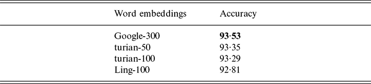
Hyperparameters: As mentioned in Section 3.2, we performed experiments with different sets of publicly published word embeddings. Table 1 gives the performance of different word embeddings on the term of 1-best accuracy. According to the results in Table 1, models using Google’s Word2vec 300-dimensional embeddings obtain a significant improvement and show that the choice of embeddings is crucial to improve the performance on this task.
Comparison of 1-best Accuracy results on the development set using different word embeddings

Abbreviations such as Google-300 refer to the Google Word2vec embeddings with a 300-dimensional embeddings space.
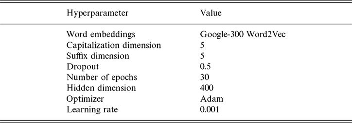
We measured the accuracy on the data set for the capitalization and suffix dimension with different values of 5, 10, 16, 32, 64 and 128. The experimental results showed that the dimension size of five achieved the highest accuracy. For the hidden dimension, we experiment with values ranging from 100 to 900 and the hidden dimension with size 400 shows the highest accuracy.
Learning algorithm: Training is done by Adam optimizer with a fixed learning rate to 0.001. We have explored other more sophisticated optimization algorithms such as Stochastic Gradient Descent and AdeDelta (Zeiler Reference Zeiler2012) without any improvement over Adam. For the output layers, we used the Softmax activation function.
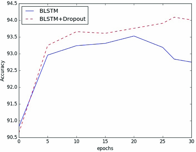
Dropout: We obtain significant improvements in our model performance after using dropout, Table 2 compare the results with and without using dropout for both development and test set; all the other parameters are the same. We observe an essential improvement in the accuracy, which demonstrates that the dropout brings significant improvement in the performance and is more effective in reducing overfitting (Pham et al. Reference Pham, Bluche, Kermorvant and Louradour2014). We used a fixed dropout rate of 0.5. We trained the models for thirty epochs; our best model was obtained at the 27th epoch. We used the model’s parameters of the highest accuracy on the development set. Figure 5 shows 1-best accuracy of our BLSTM proposed model on CCGBank section00 (development set).
1-best Accuracies results with and without dropout on development and test data

1-best accuracy of our model on CCGBank corpus Section00.

Table 3 reports the chosen hyperparameters for our best models. We tuned the hyperparameters then trained the models. We evaluate our models on term of 1-best accuracy (the most likely predicted supertag).
Final hyperparameter choice for best models

6.2 Results and analysis
6.2.1 Supertagging results
In this section, we compare our approach with the previous state-of-the-art existing models for CCG Supertagging.
Several different NN architectures have been proposed for CCG supertagging. Xu et al. (Reference Xu, Auli and Clark2015) reports the highest accuracy on development set (93.07 per cent). Besides, Lewis and Steedman (Reference Lewis and Steedman2014) (91.10 per cent) and Clark and Curran (Reference Clark and Curran2007) also reach accuracy above (92.6 per cent) with gold POS.
These three systems are considered as state-of-the-art systems in CCG Supertagging. Nevertheless, the best model accuracy reported by Xu et al. (Reference Xu, Auli and Clark2015) has access only to the previous context, while our model thanks to the strong ability of BLSTM networks can access to information in both previous and future context.
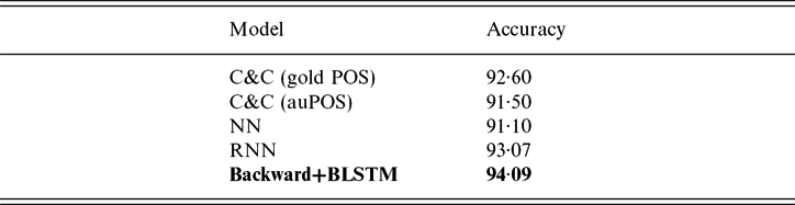
Table 4 presents 1-best accuracy (most likely predicted supertag) results of our Backward-BLSTM model on the development set comparing with all previous works. Our model produced the best performance and outperforms the C&C supertagger with gold POS (+1.5 per cent) and gives high accuracy than RNN (Xu et al. Reference Xu, Auli and Clark2015) (+1.02 per cent).
1-best accuracy on the development set (Section 00)

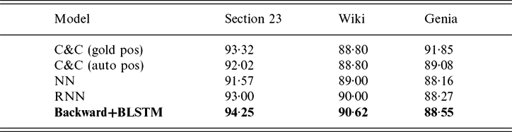
As an overall evaluation on the test set, Table 5 shows comparable testing results in terms of 1-best accuracy on Section 23 from CCGBank corpus. Our proposed supertagger significantly outperforms the state-of-the-art systems. It is clear that our supertagger is very competitive, despite using very simple architecture and a large number of CCG supertags.
1-best accuracy on the test set

Moreover, we also tested our model on two out-of-domain test set. It can be seen that our Backward-BLSTM model results are much better performance than the previous models with all test data. The only one exception is the C&C supertagger with gold-standard POS tags, in which we underperform their results in Bio-GENIA (we used Bio-GENIA gold-standard CCG lexical category data from Rimell and Clark (Reference Rimell and Clark2008) as no gold categories are available in the Bioinfer data).
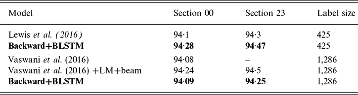
To make direct comparison with the recent works presented by Lewis et al. (Reference Lewis, Lee and Zettlemoyer2016) and Vaswani et al. (Reference Vaswani, Bisk, Sagae and Musa2016), we conduct experiments using the set of 425 labels. The results are reported in Table 6.
1-best accuracy comparison results

From Table 6, we can see that our model is no more than 0.01 per cent lower in accuracy to the model proposed by Lewis et al. (Reference Lewis, Lee and Zettlemoyer2016) on section 00 using the whole label set (1,286 label) and is (+0.12 per cent) using the set of 425 labels. This model used a deep architecture of BLSTM with a subset of 425 lexical tags. While our model achieves the same level of accuracy as Vaswani et al. (Reference Vaswani, Bisk, Sagae and Musa2016) on section 00 and is slightly lower on section 23 (−0.03 per cent). Compared with the latter our model is much simpler in term of architecture and our hidden state is thirty per cent smaller (400 versus 512). Vaswani et al. (Reference Vaswani, Bisk, Sagae and Musa2016) used a different architecture with different training procedure based on BLSTM + Language Model + beam encoding. The major differences are resumed as follow, our model introduced backward LSTM to capture long-range contextual information and eliminate the need for context windows and used BLSTM to capture information from both past and future directions.
These make our supertagger more accurate in recovering long-distance dependencies and much simpler and comparable to the recent models proposed by Lewis et al. (Reference Lewis, Lee and Zettlemoyer2016) and Vaswani et al. (Reference Vaswani, Bisk, Sagae and Musa2016).
6.2.2 Multitagging results
We also evaluate our model for multitagging, following Clark and Curran (Reference Clark and Curran2004) and Charniak et al. (1996) our CCG supertagger can potentially assign more than one supertag to a word whose probabilities are within a β factor. Categories whose probabilities are not within β factor the probability of the one-best category is pruned.
For the multitagging results, we calculate perword accuracy, where we consider the word to be tagged correctly if the correct category is included in the set of the assigned categories. We also calculate sentence accuracy which is the percentage of sentences whose words are all tagged correctly.
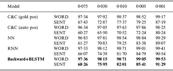
We compare our proposed model with state-of-the-art methods for multitagging. The results are reported in Table 7. In this case, it is observed that our model increases the performance of both WORD and SENT accuracy on all β levels (0.075, 0.030, 0.010, 0.005 and 0.001).
Performance comparison of different models for multitagging accuracy on Section 00 for different β levels

The WORD column gives the word accuracy and the SENT column gives the sentence accuracy.
6.2.3 Discussion
In term of learning long dependencies, LSTM gives good performance over standard RNN. Backward LSTM are very powerful in capturing past information on long time, however, the LSTMs hidden state h t takes information only from the past, knowing nothing about the future; in some cases the information in the right side is very important; the case of transitive verbs and adjectives in the English language. On the other hand, forward LSTM are very efficient on memorizing information on the left context but in some cases, it is more important to observe the previous context rather than the future one, for example in the two sentences: “I like that paint!” and “Do you want to paint?”; the word “paint” is both verb and noun, which mean that in this case it is very important to observe the previous context to determine the correct category to the word.
In sequence-labeling tasks, we have access to both left and right information context (previous and future). An analyze of our experiments results indicate the need of BLSTM to capture information on both directions.
The main findings from the direct comparison of our Backward-BLSTM model against the state-of-the-art existing models are as follows: (1) Our Backward-BLSTM model reaches a higher accuracy score. (2) it is significantly better able to train the supertagger on the full set of CCG lexical categories observed during training. However, to our knowledge other models are trained on a subset of 425 most frequent categories in CCGBank corpus. (3) It outperforms even for supertagging and multitagging.
Our main findings support the hypothesis that the LSTM-based models are more powerful in modeling sequential data. The improvements can only be due to BLSTM architecture advantages. The architecture shows consistent improvement over the best score reported on this task using standard RNN (Xu et al. Reference Xu, Auli and Clark2015).
Overall, the results we present in this paper indicates that all of our results are comparable with state-of-the-art results. Our results are promising and show that our model can compete with, and in most cases outperform.
7 Conclusion
In this paper, we demonstrated the advantages of BLSTM than simple recurrent networks for CCG Supertagging. Our proposed model outperformed previous results on supertagging and multitagging comparing to state-of-the-art models on various benchmark datasets.
In our future work, another interesting direction would be to integrate our Supertagger to the C&C parser, where the supertagger is likely to play a significant role. Additionally, the rapid success of deep learning and recurrent networks on sequence-labeling tasks leads us to believe that extensions of our model to a more complex architecture would be fruitful.