2. Experimental set-up and observations

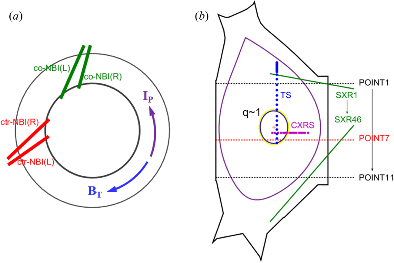
A series of experiments have been designed and carried out in the EAST tokamak, which has a rich diagnostic system and an ITER-like tungsten upper divertor (Wan et al. Reference Wan, Liang, Gong, Li, Xiang, Xu, Sun, Wang, Qian and Liu2017), to understand the influence of EPs on fishbone cycle frequency and to obtain the quantitative relationship between them. The experiments are carried with toroidal magnetic field B _t = 1.6–1.8 T, plasma current I _P = 400–500 kA, major radius R ~ 1.8 m, minor radius a ~ 0.45 m, edge safety factor q ₉₅ = 4–5 and line-averaged electron densities in the range of (3–5) × 10¹⁹ m⁻³. The NBI system in EAST (Hu et al. Reference Hu, Xie, Xie, Liu, Xu, Liang, Jiang, Sheng, Gu and Li2015) has four beam sources, with two in co-current direction and the other two in counter-current direction, which is key to demonstrate the effect of EP concentration on fishbones. Step-injected NBI power was applied to scan the pressure ratio of EPs. A sketch of the neutral beam geometry is shown in figure 1(a), in which the directions of the toroidal magnetic field and the plasma current are also labelled. Lower hybrid wave is applied to drive the plasma current and manipulate current profiles. Fishbones are confirmed by soft X-ray (SXR) (Li et al. Reference Li, Xu, Tritz, Zhu, Wan, Lan, Liu, Wei, Zhang and Hu2015) detectors and Mirnov coils. Current profiles are calculated by EFIT (Lao et al. Reference Lao, St. John, Stambaugh, Kellman and Pfeiffer1985) with the constraint of polarimeter/interferometer (Liu et al. Reference Liu, Qian, Jie, Ding, Brower, Zou, Li, Lian, Wang and Yang2016) measurements. The key diagnostics that provide the profiles of electron density, electron temperature, plasma rotation and emission signals are shown in figure 1(b).

Figure 1.

(a) The top view of the ion source layout of the NBI system of the EAST tokamak. (b) The plasma configuration during fishbone instabilities of EAST 71320 and layout of the main diagnostic systems for analysis.

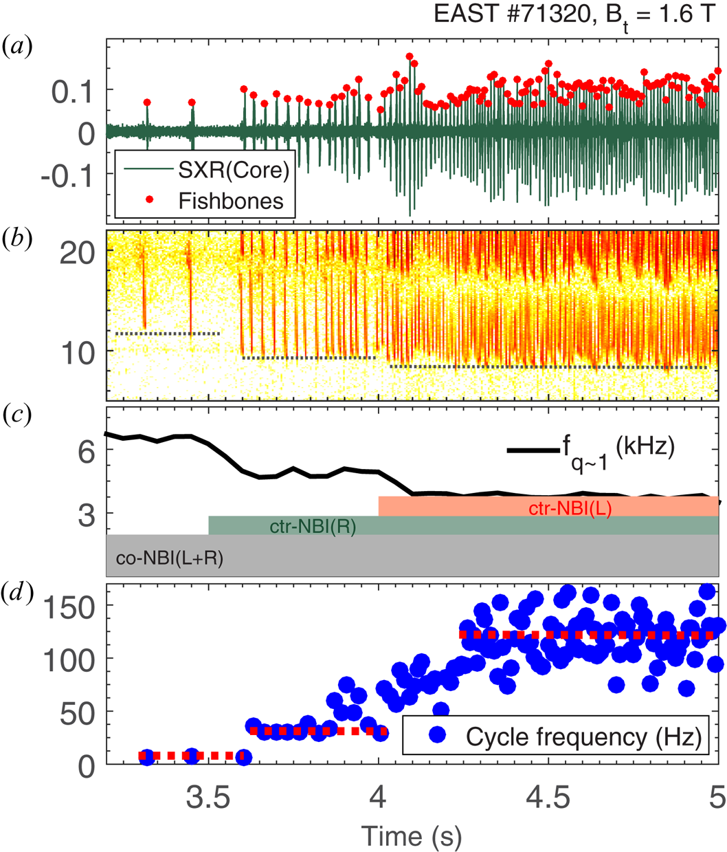
During the experiments, four neutral beam sources were injected into the plasma step by step and the co-current sources fired firstly. Fishbone instabilities were observed from both SXR detectors and Mirnov coils after the second co-current source was injected. Then with the sequential injection of the two counter-current sources, the fishbone instabilities were sustained, and the fishbone bursts became more and more frequent, as shown in figure 2(a). Meanwhile, an internal transport barrier is formed, which is beneficial for achievement of high normalized beta (β _N = 1.5–2) plasmas in EAST (Gao & The East Team Reference Gao2018).

Figure 2.

The fishbone instabilities in EAST low-magnetic-shear plasmas. (a) The signal of core SXR and (b) its time–frequency spectrum; the black dotted line is the frequency of quenching of the fishbone instability. (c) The changes of injected NBI power and the value of f _bulk-plasma at q ~ 1. (d) The cycle frequency of the fishbones.

The bursts of the fishbone instability are accompanied by downward frequency chirping, and we can see that the frequency of quenching of the fishbone decreases with the step-injected NBI power in this process, as shown in the time–frequency spectrum of SXR signal in figure 2(b). At the same time, the rotation of the core plasma decreased due to the counter-current NBI and the frequency of the bulk plasma at q ~ 1 is measured by charge exchange recombination spectroscopy (CXRS) (Li et al. Reference Li, Fu, Lyu, Du, Li, Zhang, Yin, Yu, Wang and Hellermann2014), which also shows a decline, as displayed by the black solid line in figure 2(c). These results make the trend of the frequency of fishbone in the plasma frame (f _FB = f _lab − f _bulk-plasma) (Xu et al. Reference Xu, Zhang, Chen, Hu, Li, Lin, Shi, Duan and Zhu2015) less distinguishable. A consequence of this uncertainty is the ‘inconsistency’ of the fishbone frequency dependence on EP intensity shown in figure 4 with respect to the numerical results shown in figure 8. This point is, however, not the focus of the present work, and will not be addressed in detail.

The fishbone cycle frequency (f _FC), defined by the inverse of time interval of two adjacent fishbone bursts, is used here to describe the intensity of the fishbone bursts, due to its clear positive dependence on EP intensity in the experiments. As shown in figure 2(d), the fishbone cycle frequency increased from 7 to 30 Hz and then up to 120 Hz, corresponding to three neutral beam source injections, respectively.

3. Dependence of fishbone cycle frequency on plasma parameters

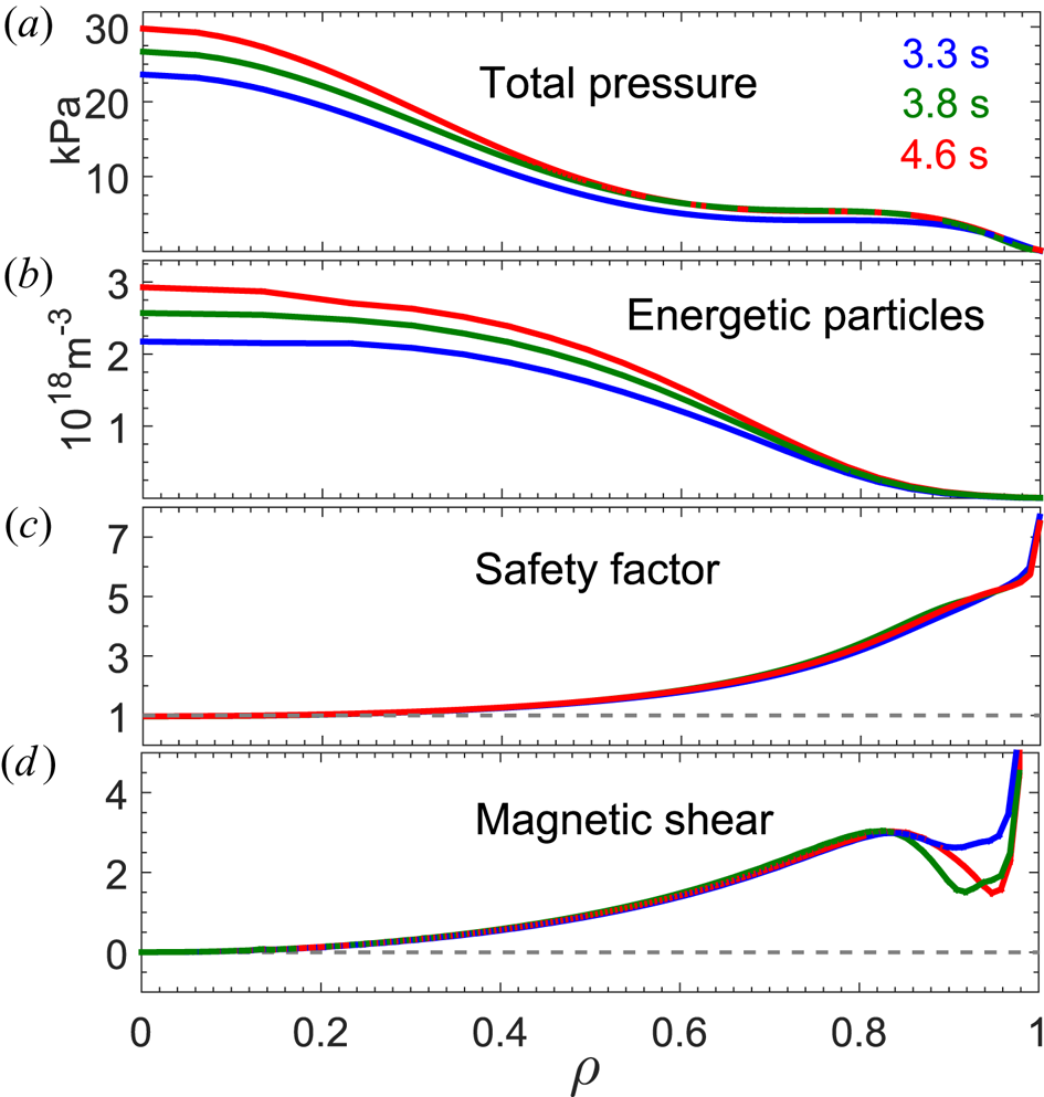
As mentioned above, the fishbones are excited when the second neutral beam source is injected into the plasma, and then the fishbone cycle frequency increases with further NBI power injection. Three typical time slices (3.3, 3.8, 4.6 s) of EAST 71320, corresponding to three NBI power injection steps, are chosen to compare the dependence of the fishbone instabilities on the plasma parameters. The SXR measurements and equilibrium results from kinetic EFIT (k-EFIT) (Li et al. Reference Li, Ren, Qian, Lao, Ding, Chen, Liu, Lu and Zang2013; Qian et al. Reference Qian, Lao, Liu, Ding, Zeng, Luo, Ren, Huang, Huang and Brower2017) show that the fishbone instability is located inside the q = 1 surface, corresponding to ρ ~ 0.15 (ρ is the square root of the normalized toroidal flux), as shown in figure 3(c). Also, with the increase of injected NBI power, the total plasma pressure increases, as shown in figure 3(a), but no clear change of the safety factor profiles in the core plasmas is observed and the magnetic shear $(s = (r/q)(\textrm{d}q/\textrm{d}r))$ is close to zero in the core region, as presented in figure 3(c,d). Here, the safety factor information presented in figure 3(c) is from the results of k-EFIT, which uses the Faraday rotation effect, density and temperature profiles measured by diagnostic systems, and experimentally measured stored energy to further improve the equilibrium, and the result will be more accurate than the one from EFIT code directly. Simulation results by TRANSP-NUBEAM (Budny et al. Reference Budny, Bell, Janos, Jassby, Johnson, Mansfield, Mccune, Redi, Schivell and Taylor1995; Pankin et al. Reference Pankin, Mccune, Andre, Bateman and Kritz2004) show that the density of EPs increases obviously with more neutral beam source injection, as shown in figure 3(b).

Figure 3.

(a) The profiles of plasma pressure. (b) Density profiles of EPs calculated by TRANSP-NUBEAM code. (c,d) Safety factor profiles and magnetic shears corresponding to fishbone instabilities under different injected NBI power steps.

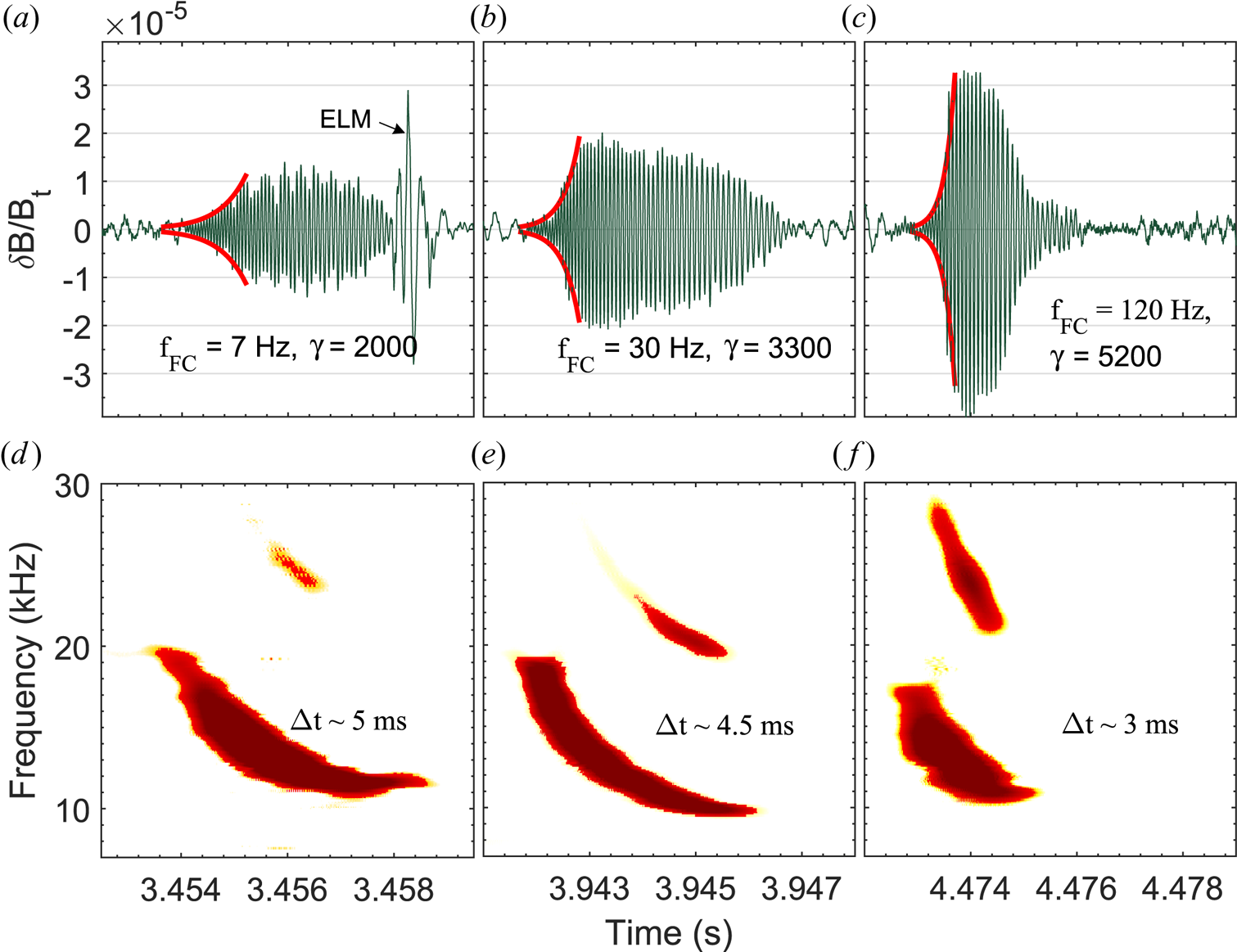
The properties of the fishbone itself are studied in this process to carry out an in-depth analysis of fishbone cycle frequency variation. The growth rates of the fishbones, described by the signal of Mirnov coils, are calculated in the same injected NBI power step and then the average taken in order to estimate the values in different power steps. Examples closest to the average growth rate of each step are presented in figure 4. It is shown that with the increase of the fishbone cycle frequency, the fishbone growth rate (γ) is increasing and the wavelet analysis of core SXR shows that the intensity of the harmonic signal of the fishbone instability is also increasing. Moreover, the width of the fishbone bursts shows a decreasing trend.

Figure 4.

(a–c) The growth rate of fishbone instabilities with different cycle frequency and (d–f) the wavelet analysis of core SXR signals. Here Δt represents the width of the fishbone duration.

For strongly driven fishbones, it is generally believed that the wave–particle interaction is the dominant nonlinearity (Zonca et al. Reference Zonca, Chen, Botrugno, Buratti, Cardinali, Cesario and Ridolfini2009). As an EP continuum mode (Chen Reference Chen1994), fishbone frequency is non-perturbatively determined by the characteristic frequency of resonant EPs; on the other hand, EPs exciting fishbones will lose energy and move radially outward, with their precessional frequency decreasing with energy. As a result, the EPs with lower energy will keep in resonance with the downward frequency chirping fishbone, and maximize power exchange with the fishbone. This is the well-known ‘mode particle pumping’ process (White et al. Reference White, Goldston, Mcguire, Boozer, Monticello and Park1983) characterizing the self-consistent fishbone nonlinear dynamics and convective EP loss, and determines other features of fishbone dynamics, e.g. the well-known fishbone cycle.

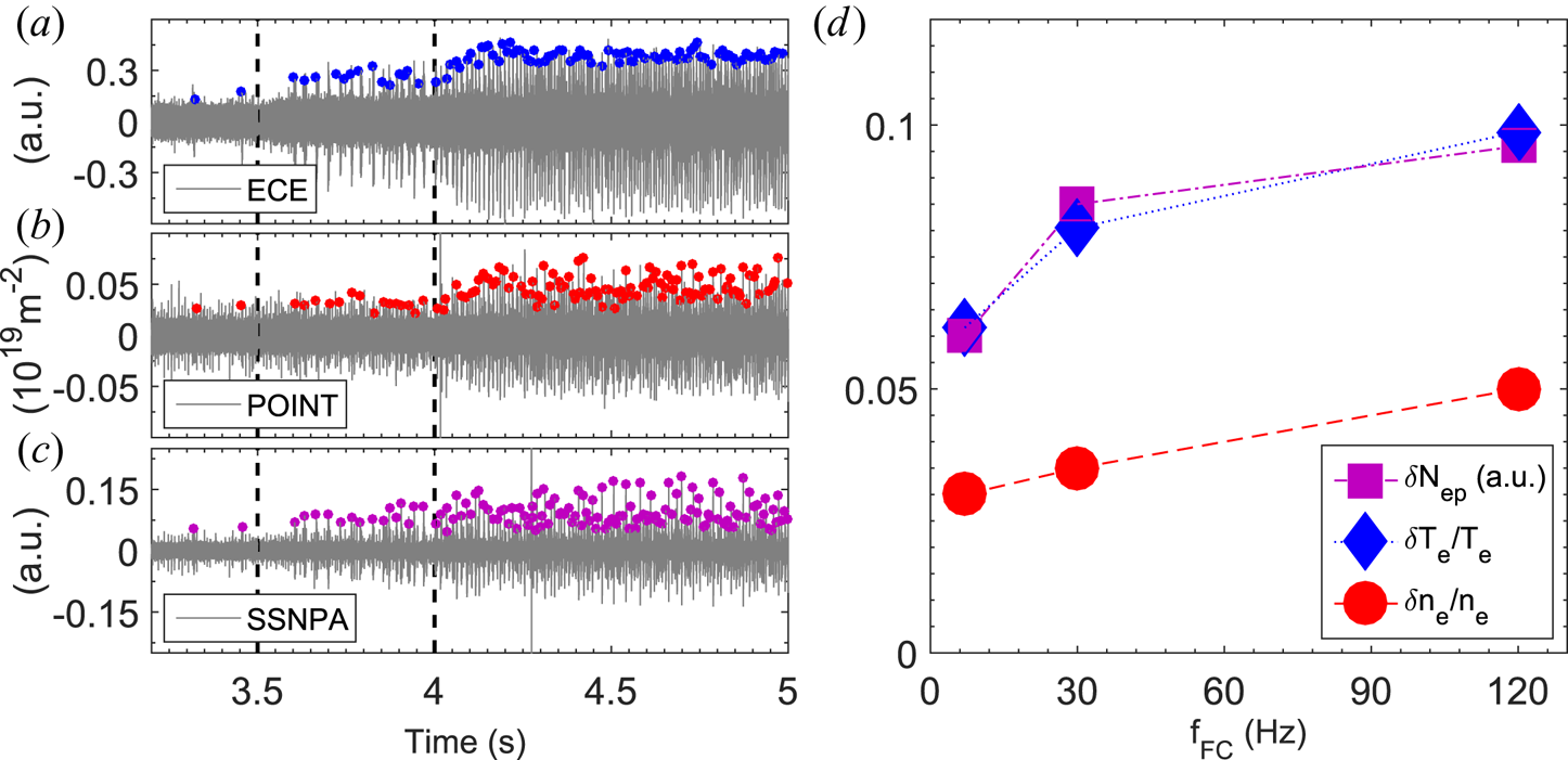
The fishbone burst will cause perturbations of plasma parameters, including the electron density, electron temperature and EP loss (White et al. Reference White, Goldston, Mcguire, Boozer, Monticello and Park1983). The dependence of increased fishbone cycle frequency on these perturbations is analysed here to evaluate its impact on the plasma performance. For the perturbation of electron density, the integral data from the polarimeter/interferometer system are used. As the fishbone instability is a local phenomenon in the core region, the perturbation is considered in the region inside the q = 1 surface, as shown in figure 1(b). The relative electron density perturbation, δn _e/n _e, is presented in figure 5(d) as red circles. The electron temperature perturbation is calculated from electron cyclotron emission (Han et al. Reference Han, Liu, Liu, Domier, Luhmann, Li, Hu and Gao2014) data, which are local measurements, and the data were checked by Thomson scattering (Zang et al. Reference Zang, Zhao, Yang, Hu, Xi, Dai, Yang, Han, Li and Hsieh2011) measurements. The results of δT _e/T _e are shown in figure 5(d) as blue diamonds. All the EP losses in these cases are considered as the result of the fishbone instability, and the amount of EP loss δN _ep is shown in figure 5(d) as purple squares. Here, the data measured by the solid-state neutral particle analyser (SSNPA) have not been absolutely calibrated, and thus we only use their relative change to characterize the change in the number of EPs ejected by the fishbones. Moreover, it is difficult to distinguish the particles that drive the fishbone instabilities among all the EPs, and we assume that the number is proportional to the total number of EPs, so we use the trend of the data from the SSNPA to characterize the relative change of EP loss caused by fishbones. Changes in the perturbations of electron density, electron temperature and amount of EP loss show that all of them increase with the fishbone cycle frequency, indicating that, with an increase of injected NBI power, more EPs will be ejected.

Figure 5.

(a–c) The filtering results of the raw data from corresponding diagnostic systems (ECE, electron cyclotron emission; POINT, polarimeter/interferometer). (d) The changes of perturbations on electron temperature, electron density and amount of EP loss by fishbone instabilities with different cycle frequency. Each data point is calculated from a large number of fishbones under the same NBI power step, and then the average result is taken.

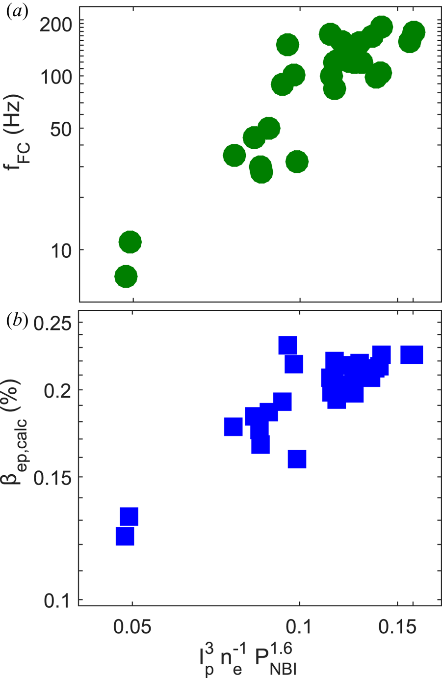
Based on the results of 71320, we also carried out a series of similar experiments, scanning a wide range of plasma currents and electron densities, and then statistics of experimental parameters of about 30 discharges were obtained. These experiments further confirmed the results of 71320. Moreover, we found that the fishbone cycle frequency has a strong dependence on three parameters: plasma current, electron density and injected NBI power. The results are shown in figure 6(a). On the other hand, according to the scaling laws of the fast ion energy rate of the EAST tokamak, from table 4 of Gu et al. (Reference Gu, Shen, Qian, Ding, Du, Sun, Xiao, Wu, Wang and Huang2019), these three parameters have a strong relationship with fishbone cycle frequency, also determining the stored energy of EPs. Thus, as we addressed before, the fishbone cycle frequency can be used as a measurement of EP drive intensity and β _ep,calc is used to characterize the strength of EP drive, assuming it is proportional to the number of EPs driving the fishbone. Here β _ep,calc is the total EP pressure ratio calculated according to the scaling laws based on the plasma parameters.

Figure 6.

The relationships between plasma parameters and fishbone cycle frequency (a) and calculated β _ep,calc (b).

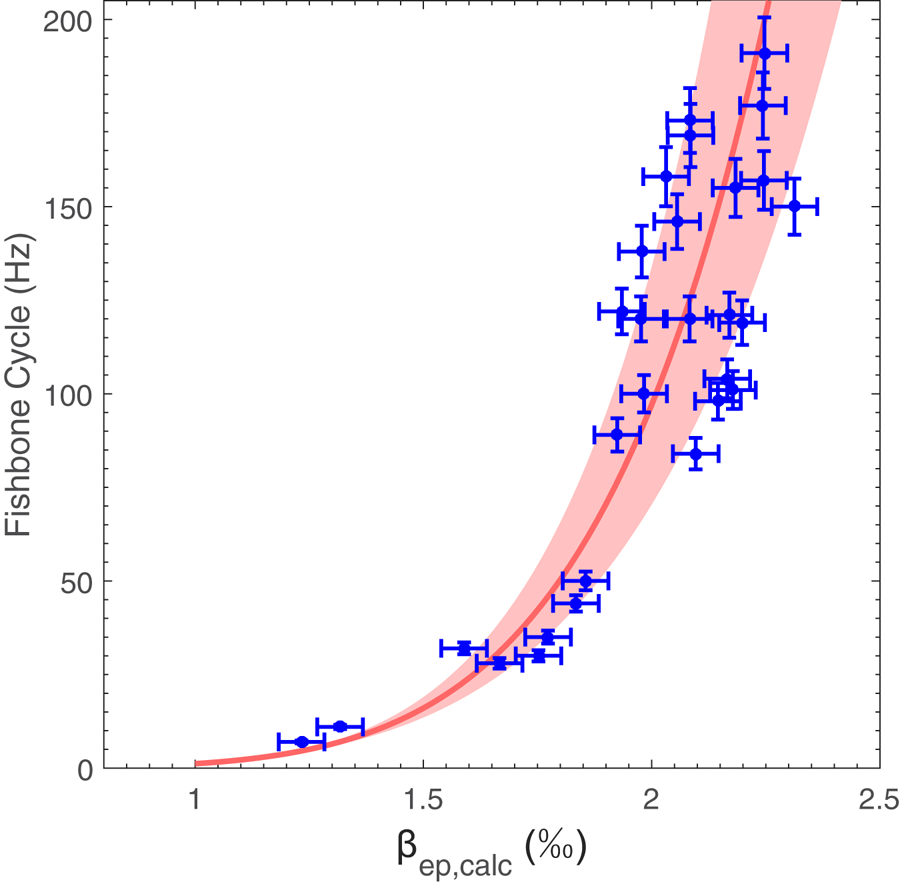
The results presented in figure 6 show a potential relationship between fishbone cycle frequency (f _FC) and β _ep,calc. To make it clear, we draw the relationship between them in figure 7 in blue circles with an error of ±5 × 10⁻⁵ for β _ep,calc and ±5 % for f _FC, then fit these results, and finally get the relationship between β _ep,calc and the fishbone cycle frequency as follows:

(3.1)\begin{equation}{f_{\textrm{FC}}} = 2.2{(1000{\beta _{\textrm{ep,calc}}} - 0.1)^{5.9 \pm 0.5}},\end{equation}

where f _FC is the fishbone cycle frequency and β _ep,calc is the pressure ratio of total EPs calculated from the scaling laws of the fast ion energy rate of the EAST tokamak. The uncertainty is represented by an index value of ±0.5 to include most of the data, as expressed by the shaded area in figure 7.

Figure 7.

The relationship between calculated β _ep,calc and fishbone cycle frequency (f _FC).

The fishbone instability starts to appear only when β _ep,calc exceeds 1‰ and f _FC > 1 Hz; as β _ep,calc continues to increase, the fishbone cycle frequency increases exponentially. Further, no saturation in fishbone cycle frequency is observed from the experimental data. One speculation is that the fishbone dynamics will qualitatively change according to the results for EAST, as the duration of each burst becomes comparable to the period between two neighbouring bursts. The power threshold for this extreme limit can be estimated from a predator–prey model, as we address in § 4.

4. Simulation analysis and model verification

Hybrid simulations with the global kinetic magnetohydrodynamics code M3D-K (Park et al. Reference Park, Belova, Fu and Tang1999; Fu et al. Reference Fu, Park, Strauss, Breslau, Chen, Jardin and Sugiyama2006) have been carried out to investigate the distribution changes of the EPs and the resonant locations. The resonance condition is given by Porcelli et al. (Reference Porcelli, Stankiewicz, Kerner and Berk1994) and expressed as

(4.1)\begin{equation}n{\omega _\phi } + p{\omega _\theta } - \omega = 0,\end{equation}

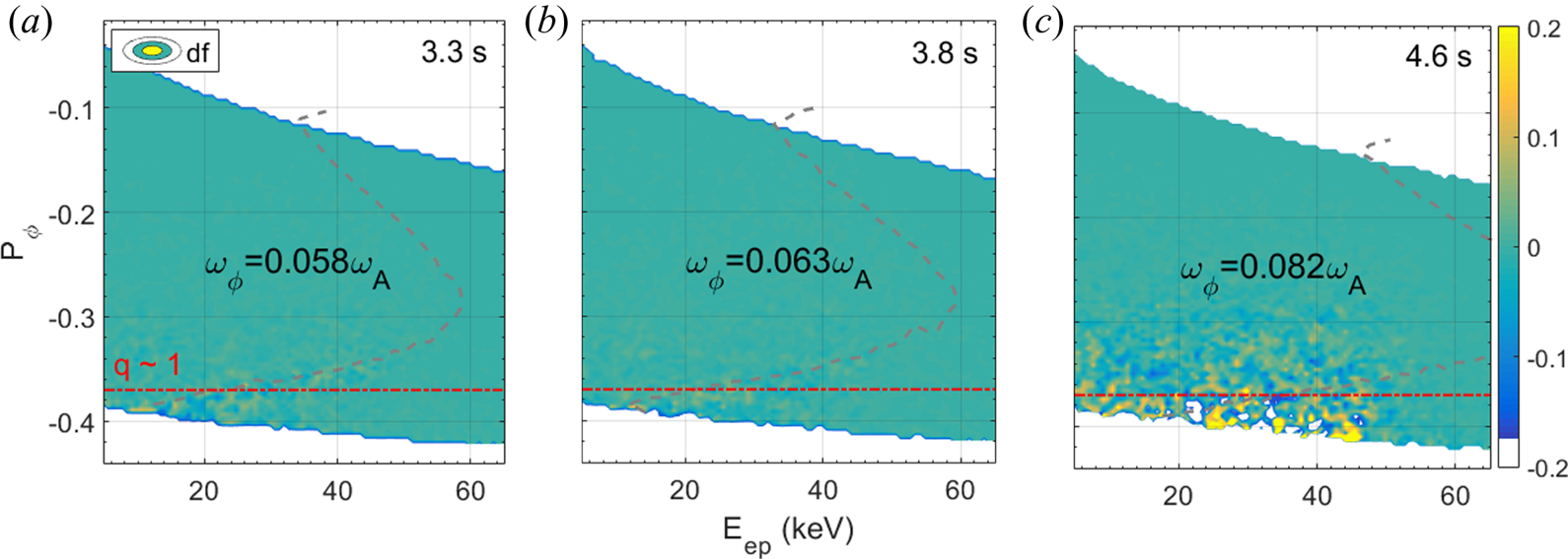
where n is the toroidal mode number, p is an integer, ω is the mode frequency, ${\omega _\theta } \equiv 2{\rm \pi} /\Delta t$ is the bounce frequency and ${\omega _\phi } \equiv \Delta \phi /\Delta t$ is the toroidal transit frequency. For the situation in this paper, n = 1 and p = 0. Figure 8 shows the EPs’ distribution change df in linear phase at three selected time slices, and the resonant locations are traced where df is significant. Parameter ${P_\phi }$ is the toroidal angular momentum expressed as ${P_\phi } = e\varPsi + M{v_{/{/}}}R{B_\phi }/B$ and represents the radial position (Shen et al. Reference Shen, Wang, Fu, Xu, Li and Liu2017), ${\omega _\phi }$ is the resonance frequency and ω _A is the Alfvén frequency. The grey dotted line gives the location of resonance condition of trapped EPs and fishbone instabilities according to calculation results.

Figure 8.

Distribution change of EPs and the resonance conditions of EPs and fishbone instabilities. The linear frequency of the fishbone increases with EP drive and approaches the precessional frequency determined by the highest energy of the NBI source, and decreases during the evolution of a single fishbone burst, due to nonlinear wave–particle interaction.

These results clearly reveal the changes of fishbone instability during the process of step-injected NBI power. With the increase of injected NBI power, the resonance conditions change in many ways. First, the resonance region tends to move towards the magnetic axis. Second, the number of resonant particles increases. And third, correspondingly, the resonance frequency is increased from 0.058ω _A to 0.063ω _A to 0.082ω _A. For the situation in this paper, considering the deeply trapped EPs, with fishbone frequency determined by EP precessional frequency, the frequency change rate can be expressed as

(4.2)\begin{equation}\dot{\omega} = \dot{\overline{{\omega _\textrm{d}}}} = \frac{{\partial \dot{{\omega _\textrm{d}}}}}{{\partial E}}\dot{E} + \frac{{\partial \dot{{\omega_\textrm{d}}}}}{{\partial r}}\dot{r},\end{equation}

with the two terms describing contributions due to energy and radial position changes, respectively, and E is the resonant EP energy and r the minor radius. For a single-n coherent mode, we have, from conservation of extended phase-space Hamiltonian $\dot{E} \approx (\omega /n){\dot{P}_\phi }$, where ${P_\phi }$ is the toroidal angular momentum and ${\dot{P}_\phi } \approx{-} {m_i}{\varOmega _i}(r\dot{r}/q)$.

Then we have

(4.3)\begin{equation}\dot{\omega } = \underbrace{{\frac{{\partial \dot{{\omega _\textrm{d}}}}}{{\partial E}}\frac{\omega }{n}\left( { - {m_i}{\varOmega_i}\frac{{r\dot{r}}}{q}} \right)}}_{\bigcirc{\kern-6pt 1}} + \underbrace{{\frac{{\partial \dot{{\omega _\textrm{d}}}}}{{\partial r}}\dot{r}}}_{\bigcirc{\kern-6pt 2}},\end{equation}

with ${\bigcirc{\kern-7pt 1}}$ and ${\bigcirc{\kern-7pt 2}}$ denoting frequency chirping due to energy and radial position changes, respectively. For weak shear, assuming $(\partial /\partial r)(q/r) \approx{-} q/{r^2}$, we have ${\bigcirc{\kern-7pt 1}}/{\bigcirc{\kern-7pt 2}}\sim r/nR \ll 1$, indicating that the radial position change is more important than the energy change in the frequency chirping.

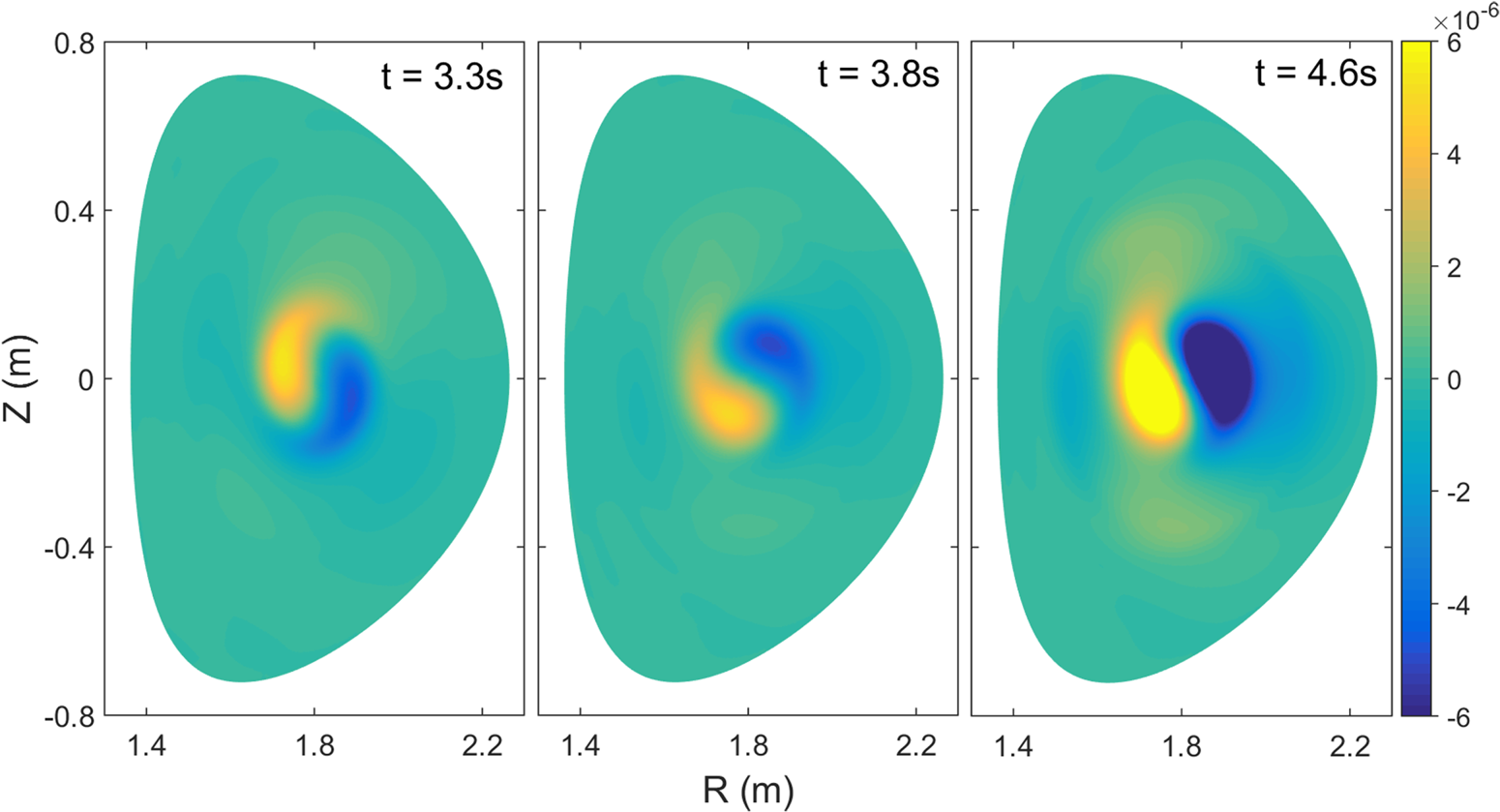
Moreover, the mode structures are also given by the simulation results from the M3D-K code, shown in figure 9, to make up for the limitations of the diagnostic systems. After the second NBI power injection, the driven EP pressure increases and exceeds β _crit, the influence on the kink mode is enhanced and becomes non-perturbative, and the structure deviates from the up–down symmetric characteristics, showing a twisted feature. At the same time, the burst of fishbone instability ejects the EPs to reduce the pressure. As more NBI power is injected, the EP pressure is further increased. Consequently, the saturation amplitude (A) and cycle frequency (f _FC) are also increased, while the width of the fishbone burst (Δt) becomes shorter.

Figure 9.

The velocity stream function $U({\epsilon ^2}{v_\textrm{A}})$ of the fishbones calculated by the M3D-K code, which is used to characterize the mode structure. Here $\epsilon \equiv a/{R_0}$ is the inverse aspect ratio and ${v_\textrm{A}}$ is the Alfvén velocity.

The above results concerning the properties of fishbone itself and the interactions between fishbone and EPs show that in the process of increasing the NBI power step by step, not only are the growth rate, frequency and structure of the fishbone itself changed, but also the conditions for its interaction with the EPs have changed. It is because of these changes that we have observed the corresponding changes of fishbone instability in the experiments.

The amount of EP loss depends on the saturation amplitude and the cycle frequency of the fishbone instability, with the former determining the amount of single burst loss and the latter determining the frequency of the loss bursts. Therefore, to evaluate the amount of EP loss caused by the fishbone instability, it is necessary to study the key factors that determine these two quantities. The resonant EP loss process, along with the mode destabilization mechanisms, allows a description of the full fishbone cycle, which has been given as a nonlinear predator–prey model (Chen et al. Reference Chen, White and Rosenbluth1984). As mentioned in the introduction, the model gives the fishbone instability properties qualitatively and shows that the energetic trapped particle pressure ratio (β _ep), which has a positive correlation with β _ep,calc, is a decisive factor for the saturation amplitude and the cycle frequency. Here, parameters consistent with the experiments are substituted into this model, expressed as $\textrm{d}A/\textrm{d}t = A\varGamma ({\beta _{\textrm{ep}}} - {\beta _{\textrm{crit}}})$ and $\textrm{d}{\beta _{\textrm{ep}}}/\textrm{d}t = D - AZ{\beta _{\max }}\varTheta ({\beta _{\textrm{ep}}} - {\beta _{\min }})$, and figure 10 shows the repetitive fishbones and the change of the fishbone cycle. The values of the relevant parameters are listed in table 1. The excitation threshold of the fishbone instability is set as 1‰ according to the experimental results in figure 7. Simulation results show that both the fishbone cycle and the width of the fishbone burst strongly depend on the change of D and β _max, which are both determined by the injected neutral beam power in the EAST tokamak. The increase of D and β _max would clearly increase the fishbone cycle frequency and decrease the width of the fishbone burst, consistent with the experimental observations, as shown in figure 10(a,c,e). Moreover, the values of A and γ are of the same order as the observed values of the Mirnov coil signals.

Table 1.

Parameter set-up in the predator–prey model in figure 10.

Figure 10.

Fishbone instabilities consistent with the experimental observations (a,c,e) and under extreme parameter regime (dotted line in b,d,f) are achieved according to the predator–prey model.

Further, as shown in figure 7, no saturation of fishbone cycle frequency has been observed in the experiments. According to the predator–prey model, a sufficiently high deposition rate of EPs (D = 2.0 s⁻¹) is assumed to study the changes in mode properties, and a fishbone cycle frequency up to about 500 Hz is obtained, as shown as a dotted line in figure 10(b,d,f). The properties of the 100 Hz fishbone are also plotted for comparison. It can be found that when the energetic trapped particle pressure ratio is high enough, the instability has a higher saturation amplitude of perturbation and a shorter duration. In such parameter regimes, the period between two fishbone bursts is almost the same as the duration of one single burst. This parameter regime is, however, quite artificial while not a typical or possible regime for the EAST tokamak. By extrapolation, it gives the upper limit on NBI power for the predator–prey model of Chen et al. (Reference Chen, White and Rosenbluth1984). And, in this extreme parameter regime, the dominant instability may change; for example, the mode can transit to a beta-induced Alfvén eigenmode with much higher frequency (Shen et al. Reference Shen, Wang, Fu, Xu, Li and Liu2017). This is, however, beyond the scope of the present work, focusing on the understanding of fishbone cycles.

5. Summary

A series of experiments have been designed and carried out on the EAST tokamak to study the dependence of fishbone cycle frequency on EPs. High normalized beta (β _N = 1.5–2) plasmas with edge transport barrier and internal transport barrier were achieved, and fishbone instabilities with different cycle frequencies were observed. Detailed analysis shows that with an increased injected NBI power, not only have the properties of the fishbone itself changed, such as growth rate, frequency and mode structure, but also the resonance conditions between the fishbone mode and the EPs have changed, like resonance region, number of resonant particles and resonant frequency. The plasma current profiles, which are controlled by appropriate lower hybrid wave injection, keep almost constant, showing q ₀ ~ 1 and the relative magnetic shear is close to zero.

Through a series of experiments conducted on EAST with numerical simulations, we clearly showed the process of the fishbone cycle frequency changes, and obtained the relationship between cycle frequency and the calculated pressure ratio of total EPs as ${f_{\textrm{FC}}} = 2.2{(1000{\beta _{\textrm{ep,calc}}} - 0.1)^{5.9 \pm 0.5}}$. According to the predator–prey model and substituting the estimated experimental data into it, fishbones that are in agreement with the experimental observations have been achieved. These results confirm the previous analysis that the key factor affecting the fishbone cycle frequency is the EP pressure ratio, which is dominated by the input power of the NBI system. Results in this paper will provide an important basis for EAST to explore advanced scenarios.

The excitation threshold of the fishbone instability considered here is not changed in the calculations, which still requires more experiments and analysis to confirm. Moreover, the quantitative relationship between fishbone cycle and EPs in the EAST tokamak, which shows that the fishbone cycle frequency increases with increasing beam power, is contrary to the results for the PDX and DIII-D devices. Future work is needed to understand that.