1 Introduction
An axisymmetric self-preserving wake pattern has long been supposed to be a universal feature of a far wake independent of the axisymmetric bluff-body configuration (e.g. George Reference George, George and Arndt1989). Johansson, George & Gourlay (Reference Johansson, George and Gourlay2003) investigated theoretically the equilibrium similarity of the axisymmetric wake and proposed that the transverse length scale, i.e. the wake width, should grow as
 $x^{1/3}$
, whereas the maximum velocity deficit should decrease as
 $x^{-2/3}$
, where
 $x$
is measured in the flow direction. This self-similarity law has appealing prospects, but, admittedly, its universal validity is still an open question.
The proposed self-similarity law has been proved for the wake behind an axisymmetric disk (Johansson et al. Reference Johansson, George and Gourlay2003; Johansson & George Reference Johansson and George2006). Rather unexpectedly, the same self-similarity was observed experimentally in the far wake behind a three-blade rotor which can be axisymmetric only in two limiting cases: for an infinite number of blades or for rotor rotation at infinite speed (Okulov et al. Reference Okulov, Naumov, Mikkelsen and Sørensen2015). It was suggested that the universality of the self-similarity law might have the possibility to apply also for abnormal axisymmetric wakes, thereby inspiring investigations of different types of wakes. Unfortunately, however, the modest velocity deficit and its slow decay rate make accurate measurements in axisymmetric far wakes difficult. Okulov et al. (Reference Okulov, Naumov, Mikkelsen and Sørensen2015), for instance, were unable to obtain sufficiently detailed flow field data to calculate the integral parameters and thereby to directly verify the similarity law.
A direct numerical simulation (DNS), on the other hand, provides detailed three-dimensional flow fields which enable in-depth explorations of the wake topology. We recently simulated the wake behind an inclined prolate spheroid and observed that the steady laminar wake at Reynolds number
 $Re_{D}=1000$
(Jiang, Gallardo & Andersson Reference Jiang, Gallardo and Andersson2014) evolved into a highly asymmetric transitional wake at
 $Re_{D}=3000$
(Jiang et al.
Reference Jiang, Gallardo, Andersson and Zhang2015). In the latter case, a surprisingly coherent vortex tube could be observed and this persistent vortex tube exhibited a helical nature (Alekseenko et al.
Reference Alekseenko, Kuibin, Okulov and Shtork1999; Alekseenko, Kuibin & Okulov Reference Alekseenko, Kuibin and Okulov2007). The helical vortex tube was the single most dominant feature of the wake flow and its peculiar features will be scrutinized in the present communication.
The validity of the self-similarity law for asymmetric wakes behind non-axisymmetric bodies has never been addressed. Our primary purpose is to examine the self-similarity of the coherent vortex tube in the far wake behind the inclined spheroid to partially fill this knowledge gap. A subsidiary goal of the study is to provide a detailed description of how the helical vortex evolves from the nearest wake to the transitional far wake, including phenomena such as a complex vortex composition and an abrupt transition of helical symmetry from right- to left-handed (Okulov Reference Okulov1996; Alekseenko et al. Reference Alekseenko, Kuibin and Okulov2007) which might be related to a vortex breakdown but with no flow reversal (Sarpkaya Reference Sarpkaya1971; Faler & Leibovich Reference Faler and Leibovich1977; Leibovich Reference Leibovich1978, Reference Leibovich1984). The study intentionally focuses only on one flow configuration in order to provide an in-depth analysis of the flow physics of that particular wake. The flow problem considered is, however, a three-parameter problem, but it is beyond the scope of the present study to explore how the wake topology varies throughout parameter space.
2 Flow configuration and computational approach
We consider the flow around a prolate spheroid with aspect ratio 6:1, inclined
 $45^{\circ }$
with respect to the uniform flow. The Reynolds number
 $Re_{D}=U_{0}D/{\it\nu}=3000$
where
 $U_{0}$
is the velocity of the oncoming flow and
 $D$
is the minor axis of the spheroid.
The incompressible flow is governed by the mass conservation and Navier–Stokes equations which are integrated forward in time on a
 $38D\times 24D\times 21D$
computational domain. Three different Cartesian meshes are considered and the finest mesh comprises
 $1344\times 1024\times 544$
grid points which amount to
 $749\times 10^{6}$
cells. The finite-volume solver MGLET (Manhart Reference Manhart2004) is utilized to conduct the simulations and no-slip and impermeability conditions are enforced at the surface of the spheroid by means of a direct-forcing immersed boundary method (IBM) due to Peller et al. (Reference Peller, Le Duc, Tremblay and Manhart2006). Further information about computational issues, including a detailed grid refinement test, were provided by Jiang et al. (Reference Jiang, Gallardo, Andersson and Zhang2015). The same computational approach has recently been used by El Khoury, Andersson & Pettersen (Reference El Khoury, Andersson and Pettersen2010), Gallardo, Andersson & Pettersen (Reference Gallardo, Andersson and Pettersen2014) and Jiang et al. (Reference Jiang, Gallardo and Andersson2014, Reference Jiang, Gallardo, Andersson and Zhang2015) for three-dimensional wake flow problems.
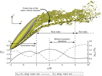
Perspective view of the wake visualized by the isosurface of
 ${\it\lambda}_{2}=-20$
. The axis of the main vortical structure is marked as a broken black line. The mean axial velocity
 $\langle u_{ax}\rangle /U_{0}$
and the mean pressure coefficient
 $\langle C_{p}\rangle =(\langle p\rangle -p_{0})/0.5{\it\rho}U_{0}^{2}$
(where
 $p_{0}$
is the reference pressure at the inlet) are plotted along the vortex centre line from the inception
 $x/D=-2$
up to
 $x/D=+10$
. The depicted axes
 $x^{\prime }$
and
 $y^{\prime }$
are aligned with the corresponding axes of the global coordinate system
 $(x,y,z)$
with its origin in the centre of the spheroid.

3 The coherent helical vortex structure
The three-dimensional wake which develops behind the inclined spheroid is depicted in figure 1. At a significantly lower
 $Re_{D}=1000$
, the laminar wake consisted of a pair of counter-rotating vortices of unequal strength (Jiang et al.
Reference Jiang, Gallardo and Andersson2014). In the present transitional wake, despite numerous small turbulent-like structures, a single vortex tube is apparently the most dominant coherent structure and will accordingly be referred to as the main vortical structure. This helical vortex originates from one part of the vortex pair shed from the lower part of the forebody of the spheroid. The other part of the vortex pair breaks and disrupts at an early stage of the wake and is scarcely visible in figure 1. Details of the near wake have been reported by Jiang et al. (Reference Jiang, Gallardo, Andersson and Zhang2015), whereas the present paper reports on an in-depth exploration of the dominant helical vortex tube all the way into the far wake.
The helical vortex is not a straight tube all through the wake. In the lee of the spheroid, the vortex tube is partially aligned with the bluff-body geometry with an inclination somewhat below
 $45^{\circ }$
. As the vortex tube leaves the shadow of the spheroid, however, it is immediately bent by the free stream and at the same time deflected to the right. This sideways distortion is associated with the asymmetries of the entire wake. In order to investigate the details of the vortex, we introduce a local cylindrical coordinate system with its origin along the vortex centre line and one coordinate direction in the local axial direction. Radial and azimuthal directions are defined in the cross-section perpendicular to the local axial direction. The velocity field originally computed in the Cartesian coordinate directions is therefore transformed to the local cylindrical coordinate system, i.e.
 $\boldsymbol{U}=(u_{ax},u_{{\it\theta}},u_{r})$
, to enable further analysis.
To facilitate the forthcoming discussions, three different stages of the development of the main vortex structure can be identified from the variation of the axial velocity and pressure in figure 1. Stage 1: the first stage
 $-2<x/D<+2$
can be regarded as the generation stage. The fluid passes over the side of the spheroid and sheds to form a vortex sheet which eventually rolls up to form the helical vortex tube; Stage 2: in the near wake
 $+2<x/D<+8$
we will see that an abrupt change in the vortex core occurs, accompanied by a sudden change of axial velocity profile and helical symmetry; Stage 3: in the far wake
 $x/D>+8$
the axial velocity in the vortex tube remains wake-like and the self-similarity laws proposed by Johansson et al. (Reference Johansson, George and Gourlay2003) apply.
3.1 Stage 1 – vortex generation
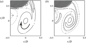
The vortex sheets shed from the separation lines along the spheroid discharge vorticity to generate vortical structures in the near wake. At the high inclination angle considered here, the separation lines are also inclined with respect to the free stream. The newly generated vortices are therefore inclined almost similarly as the spheroid. Since the main vortex is generated at the right side of the spheroid, it has positive axial vorticity
 $\langle {\it\omega}_{ax}\rangle D/U_{0}$
as shown in figure 2(a). The axial vorticity is the dominant component of the vorticity vector and retains the same positive sign all along the vortex tube (to be shown in the following subsection).
Vorticity in the cross-sectional plane perpendicular to the vortex axis at
 $x/D=+1$
. The vortex centre is at the origin
 $r/D=0$
and the bold arrow indicates the clockwise rotation associated with the helical motion. (a) Distribution of axial vorticity
 $\langle {\it\omega}_{ax}\rangle D/U_{0}$
; (b) distribution of azimuthal vorticity
 $\langle {\it\omega}_{{\it\theta}}\rangle D/U_{0}$
. Solid and dashed contour lines represent positive and negative values, respectively. The shadowed region in the upper left corner is a rough representation of the bluff body.
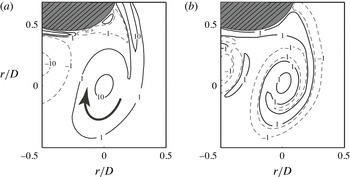
One can immediately see from figure 2 that the axial vorticity component is far larger than the magnitude of the azimuthal vorticity component. However, it is interesting to see the azimuthal vorticity distribution in figure 2(b) which reflects a so-called vortex composition phenomenon, i.e. positive and negative azimuthal vorticity interacting and spiralling together. The vortex composition in the present case is complex with multiple alternations between right- and left-handed swirl in the vortex core. Alekseenko et al. (Reference Alekseenko, Kuibin, Okulov and Shtork1999) first described the vortex composition phenomenon in a swirling flow generated by a vortex generator, but with only one alteration, as seen in their figure 17. In the present case of the streamlined body, the negative azimuthal vorticity in figure 2(b) is generated at the front side of the spheroid and the positive azimuthal vorticity is generated at the leeward side of the spheroid. The composition phenomenon observed in figure 2(b) is thus a result of interactions between sheets of azimuthal vorticity of opposite signs originating from two different parts of the spheroidal body. It is noteworthy that vortex composition can be seen all through the vortex generation stage, but disappears in the near wake.
3.2 Stage 2 – alteration of helical symmetry in the vortex core
The newly formed vortex tube develops with roughly the same inclination as the bluff body until
 $x/D\approx 2$
. However, the vortex tube is unable to align with the spheroid all the way to the upper pole, as seen in figure 1. As soon as the vortex tube leaves the shadow of the spheroid, the tube is bent by the free stream so that the inclination of the vortex axis with respect to the
 $x$
-direction is reduced to approximately
 $10^{\circ }$
. The variations of the axial velocity
 $\langle u_{ax}\rangle$
and the pressure coefficient
 $\langle C_{p}\rangle$
in the lower part of figure 1 show that the pressure and the axial velocity attain local maximum and minimum values, respectively, at approximately
 $x/D\approx 2$
where the vortex tube is being bent. This is indeed a reflection of the continuous bending of the vortex tube caused by the free stream. Nevertheless, the vortex is able to retain its coherence after this stage.
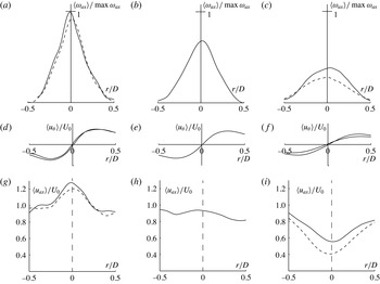
Profiles of axial vorticity (a–c), azimuthal velocity (d–f) and axial velocity (g–i) along a diameter of the vortex cross-section. (a,d,g) Results at
 $x/D=4$
and 5 before the helical symmetry alteration; (b,e,h) at
 $x/D=6$
during the alteration; and (c,f,i) at
 $x/D=7$
and 8 after the alteration.

Major changes in the vortex topology occur in the near wake from
 $x/D=4$
to
 $x/D=8$
, as seen in figure 3 where the velocity and vorticity variations across the vortex tube are shown at five different cross-sections. Let us first consider the jet-like profiles of the axial velocity
 $\langle u_{ax}\rangle$
at
 $x/D=4$
and 5 shown in figure 3(g). It is noteworthy that the maximum value of
 $\langle u_{ax}\rangle$
at the vortex centre even exceeds the free-stream velocity
 $U_{0}$
by some 20 %. Such jet-like profiles are unexpected in the near wake of the inclined spheroid since we are not aware of any earlier observations of jet-like velocity profiles in three-dimensional wakes from which wake-like profiles are normally reported. Jet-like profiles are important, however, because birds and fishes move very effectively leaving such wake profiles behind (Taylor et al.
Reference Taylor, Liberzon, Gurka, Holzman, Reesbeck and Diez2013). To the authors’ best knowledge, jet-like profiles in a near wake have only been seen in conjunction with two-dimensional von Kármán streets (Taylor et al.
Reference Taylor, Liberzon, Gurka, Holzman, Reesbeck and Diez2013). The jet-like profiles seen in figure 3(g) are unforeseen and probably caused by three-dimensional effects in the near wake.
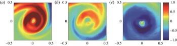
Azimuthal vorticity
 $\langle {\it\omega}_{{\it\theta}}\rangle D/U_{0}$
over three different vortex cross-sections. (a) At
 $x/D=5$
and before the helical symmetry alteration. (b) At
 $x/D=6$
and during the alteration. (c) At
 $x/D=7$
and after the alteration.

From the jet-like velocity profile at
 $x/D=5$
in figure 3(g) the flow field experiences a sudden change to the wake-like variation at
 $x/D=7$
in figure 3(i). This change is accompanied by a change of the sign of azimuthal vorticity shown in figure 4. At
 $x/D=5$
in figure 4(a), the azimuthal vorticity is positive all over the vortex core and the positive
 $\langle {\it\omega}_{{\it\theta}}\rangle$
corresponds with the jet-like
 $\langle u_{ax}\rangle$
in figure 3(g). At
 $x/D=7$
in figure 4(c), the azimuthal vorticity has become distinctly negative within the vortex core, corresponding to the wake-like axial velocity profile in figure 3(i). In between, i.e. at
 $x/D=6$
, we cannot observe any particular dominating sign of azimuthal vorticity in figure 4(b). Indeed, the axial velocity profile in figure 3(h) shows that
 $\langle u_{ax}\rangle$
is roughly uniformly distributed over this vortex cross-section. According to Alekseenko et al. (Reference Alekseenko, Kuibin, Okulov and Shtork1999), a helical vortex with positive azimuthal vorticity is a right-handed vortex while one with negative azimuthal vorticity is a left-handed vortex. The plots of figures 3 and 4 suggest a change in helical symmetry of the vortex core from right to left (Okulov Reference Okulov1996; Martemianov & Okulov Reference Martemianov and Okulov2004).
The switching from a right-handed to a left-handed helical vortex is usually accompanied by a change of axial velocity profile, just as we observed in the present study. Okulov (Reference Okulov1996) and Martemianov & Okulov (Reference Martemianov and Okulov2004) associated such a change of the vorticity distribution together with the formation of a flow reversal in the vortex centre as a ‘classical’ vortex breakdown (Leibovich Reference Leibovich1978; Alekseenko et al.
Reference Alekseenko, Kuibin and Okulov2007). However, figure 3(g–i) shows no negative values of the axial velocity; i.e. no recirculation bubble with stagnation points separating flows in opposite directions exists. For low Reynolds number flows at relatively low swirl levels Sarpkaya (Reference Sarpkaya1971) and Faler & Leibovich (Reference Faler and Leibovich1977) observed a similar phenomenon. Nevertheless, the abrupt changes of the present vortex flow represents an original form of abrupt change of helical symmetry in which the switch from a right to left helix at
 $x/D\approx 6$
is not accompanied by a flow reversal.
Martemianov & Okulov (Reference Martemianov and Okulov2004) derived several different axial velocity profiles (see figure 2 in their paper) that may occur in a continuous vortex tube with operating conditions under the same flow integrals. Abrupt changes of different velocity profiles may appear from the same initial vortex structures with right-handed helical symmetry, e.g. the ‘classical’ vortex breakdown takes place when the original jet-like profile switches to a wake-like variation, together with a negative axial velocity at the vortex axis. However, their theoretical analysis also hypothesized other possible scenarios in which transition between different profiles might occur without a flow reversal. A transition between two wake-like profiles was observed experimentally by Velte, Okulov & Hansen (Reference Velte, Okulov and Hansen2011) and referred to as a ‘slight’ alteration of helical symmetry from one left-handed to another left-handed helical symmetry, accompanied by an expansion of the vortex core but without changes in flow topology. This so-called ‘slight’ alteration is different from the ‘classical’ vortex breakdown with the symmetry changing from right to left. The present vortex tube, however, experiences a sudden change between jet- and wake-like profiles as the right-handed helix transforms to a left helix, while maintaining a positive axial velocity without any flow reversal (i.e. without any change of flow topology as in the ‘slight’ case, but with strong change of helical symmetry like the ‘classical’ one). This phenomenon might be similar to the one visualized by Sarpkaya (Reference Sarpkaya1971) and Faler & Leibovich (Reference Faler and Leibovich1977), although they did not report on any alteration of the helical symmetry. The present vortex alteration associated with the changing of helical symmetry is therefore qualitatively different from both classical and slight alterations in the vortex core. Although the possible existence of this type of symmetry alteration was postulated by theoretical considerations (Martemianov & Okulov Reference Martemianov and Okulov2004; Okulov & Sørensen Reference Okulov and Sørensen2010), it has never been documented and analysed in a real vortex core. Let us therefore proceed to explore this phenomenon in greater detail.
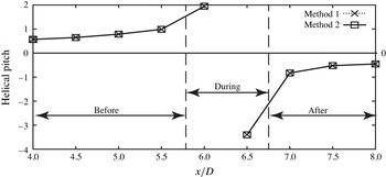
Variation of the helical pitch
 $l$
along the axis of the vortex tube. The numerical values obtained with the two different methods are almost indistinguishable.

Okulov (Reference Okulov1996) first pointed out that a vortex breakdown is essentially a change of the helical symmetry in the vortex core, which implies a change of sign of the helical pitch. The pitch
 $l$
can be used for identification of vortex breakdown in combination with examinations of the velocity and vorticity distributions, as in figures 3 and 4. Alekseenko et al. (Reference Alekseenko, Kuibin, Okulov and Shtork1999) proposed several alternative approaches to estimate the vortex pitch in swirling flow devices. More recently Velte, Hansen & Okulov (Reference Velte, Hansen and Okulov2009) applied two of these methods to estimate the helical pitch for vortex structures in unbounded turbulent flows. The first method obtains
 $l$
by minimizing the residual of
 $u_{ax}+(r/l)u_{{\it\theta}}=u_{a}(x)$
, where
 $u_{a}$
is the vortex advection velocity, in a least-square sense. In the second method
 $l$
is calculated from
 $l=-F_{mm}/(F_{m}-u_{a}G)$
where
 $F_{mm}=\int _{{\it\Sigma}}{\it\rho}u_{{\it\theta}}u_{ax}r\,\text{d}{\it\Sigma}$
, with
 $F_{m}=\int _{{\it\Sigma}}{\it\rho}u_{ax}^{2}\,\text{d}{\it\Sigma}$
and where
 $G$
is the mass flow rate. Results obtained with both methods are seen to collapse in figure 5. It is of particular interest to observe that the helical pitch
 $l$
is positive before
 $x/D=6$
where the axial velocity distribution is jet-like and the azimuthal vorticity has positive values. On the contrary,
 $l$
is negative downstream of
 $x/D=7$
where the axial velocity profile has changed to wake-like and the azimuthal vorticity became negative. Okulov, Sørensen & Voigt (Reference Okulov, Sørensen and Voigt2005) studied the way of change of the helical pitch during a vortex breakdown. They predicted and discovered that, despite the traditional picture in which a vortex ring acquires zero pitch in the limit, the transition may also occur when it acquires infinite pitch
 $l$
. The variation of
 $l(x)$
in figure 5 suggests that the scenario outlined by Okulov & Sørensen (Reference Okulov and Sørensen2010) occurs in the present case.
The fact that the helical pitch
 $l$
exhibits a sudden change from positive to negative sign provides further evidence that the main vortex in this complex three-dimensional wake experiences a helical symmetry alteration process, although the flow topology is unchanged. As already mentioned, an atypical form of a ‘slight’ vortex alteration was reported from the experimental study by Velte et al. (Reference Velte, Okulov and Hansen2011) in which the flow topology remained unchanged. In their case also the wake-like form of the axial velocity profile remained the same although the helical pitch changed abruptly. In the present study, however, another kind of symmetry transformation in the vortex core has been identified. Changes of the vortex helical parameters appear with a transition from jet-like to wake-like axial velocity profile, but without a change in flow topology (no flow reversal at the vortex axis). To the authors’ best knowledge, this is the first time that this vortex alteration scenario is detected and analysed.
3.3 Stage 3 – self-similarity in the far wake
The essential features of the coherent vortex structure are preserved through the far wake, i.e. downstream of
 $x/D\approx 8$
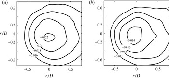
and all the way to the outlet of the computational domain. This is so for the positive axial vorticity, the negative azimuthal vorticity and the wake-like axial velocity profiles. Moreover, the vortex tube exhibits an almost axisymmetric shape, as demonstrated by the pressure coefficient contours at
 $x/D=21.5$
and 26 in figure 6. These plots are cross-sections through the main coherent vortex structure in which a significant fraction of the wake energy is concentrated. Although these data are taken far downstream of the part of the wake shown in figure 1, a distinct pressure minimum is observed at the vortex centre.
Contours of the pressure coefficients
 $\langle C_{p}\rangle$
in the far wake. Both plots are centred at the local vortex centre. (a) At
 $x/D=21.5$
; (b) at
 $x/D=26$
.

In this subsection, the validity of the self-similarity laws mentioned in the Introduction will be assessed. This is motivated by the hypothesized universality of the laws also for abnormal axisymmetric cases (Okulov et al.
Reference Okulov, Naumov, Mikkelsen and Sørensen2015). According to the theory of Johansson et al. (Reference Johansson, George and Gourlay2003) the evolution of the maximum velocity deficit
 $U_{def}=(U_{0}-u_{ax})_{max}$
along the vortex axis and the transverse length scale
 ${\it\delta}_{\ast }$
of the axisymmetric vortex tube should follow the self-similarity laws:
 $$\begin{eqnarray}{\it\delta}_{\ast }/{\it\theta}=a[(x-x_{0})/{\it\theta}]^{1/3};\quad U_{def}/U_{0}=b[(x-x_{0})/{\it\theta}]^{-2/3},\end{eqnarray}$$
where
 ${\it\theta}$
(the momentum thickness) and
 ${\it\delta}_{\ast }$
(the transverse length scale) are defined as:
 $$\begin{eqnarray}{\it\theta}^{2}=\lim _{\tilde{r}\rightarrow \infty }\frac{1}{U_{0}^{2}}\int _{0}^{\tilde{r}}u_{ax}(U_{0}-u_{ax})r\,\text{d}r;\quad {\it\delta}_{\ast }^{2}=\lim _{\tilde{r}\rightarrow \infty }\frac{1}{U_{def}}\int _{0}^{\tilde{r}}(U_{0}-u_{ax})r\,\text{d}r.\end{eqnarray}$$
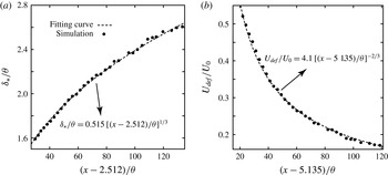
Data for
 ${\it\delta}_{\ast }/{\it\theta}$
versus
 $(x-x_{0})/{\it\theta}$
and
 $U_{def}/U_{0}$
versus
 $(x-x_{0})/{\it\theta}$
are deduced from the simulated flow field in the range between
 $x/D=9$
to 26 and plotted as black dots in figures 7(a) and 7(b), respectively. The broken lines are the best-fit curves:
 $$\begin{eqnarray}\displaystyle & \displaystyle {\it\delta}_{\ast }/{\it\theta}=0.515[(x-2.512)/{\it\theta}]^{1/3}, & \displaystyle\end{eqnarray}$$
 $$\begin{eqnarray}\displaystyle & \displaystyle U_{def}/U_{0}=4.1[(x-5.135)/{\it\theta}]^{-2/3}. & \displaystyle\end{eqnarray}$$
The results in figure 7 follow the self-similarity laws with the particular power-law variation in (3.1) exceptionally well. It is furthermore interesting to note that the best-fit coefficients
 $a=0.515$
,
 $b=4.1$
in (3.3) and (3.4) give
 $ab=1.087$
. This value is only 8.7 % above the constraint
 $ab=1$
proposed by Johansson & George (Reference Johansson and George2006). They also mentioned that the virtual origin
 $x_{0}$
should be the same in both (3.1). The present results are different in this respect since
 $x_{0}$
in (3.4) is almost exactly twice the value of
 $x_{0}$
in (3.3), i.e.
 $5.135/2.512\approx 2.04$
. In the wake behind a single disk, Johansson & George (Reference Johansson and George2006) considered the entire wake. The present study is, on the other hand, focusing only on the main vortex structure. Although this vortex structure is the most dominant feature of the present wake flow, it is nevertheless only a part of the entire wake behind the spheroid. In fact, the vortex tube under consideration here stemmed from half of the vorticity shed from the inclined spheroid. This might explain the difference between our results and those of Johansson & George (Reference Johansson and George2006). Another explanation may be associated with the more complex vortex composition reported in § 3.1. Discussions by Alekseenko et al. (Reference Alekseenko, Kuibin, Okulov and Shtork1999) suggested that vortex composition can either reduce the velocity in the vortex core or change the real vortex size.
(a)
 ${\it\delta}_{\ast }/{\it\theta}$
versus
 $(x-x_{01})/{\it\theta}$
, where
 $x_{01}=2.512$
; (b)
 $U_{def}/U_{0}$
versus
 $(x-x_{02})/{\it\theta}$
, where
 $x_{02}=5.135$
. The black dots are calculated values based on the simulation data and dashed lines are best-fit curves obeying the power-law variations (3.1) proposed by George (Reference George, George and Arndt1989).

4 Summary and concluding remarks
An in-depth exploration of the main vortical structure in the transitional wake behind a
 $45^{\circ }$
inclined 6:1 prolate spheroid at Reynolds number 3000 has been undertaken. This main vortical structure is the only persistent coherent vortex tube in the three-dimensional transitional wake. The vortex tube has been identified as a helical vortex which is bent by the free stream as it leaves the shadow of the spheroid. To facilitate the analysis of the flow field and the accompanying interpretations, we introduced a local cylindrical coordinate system with one coordinate axis along the curved vortex centre line.
The helical vortex originated from a vortex sheet shed from the separation line at the spheroidal surface. In the generation stage, a new form of vortex composition phenomenon with several alterations between right and left helix was seen. This topology is more complex than the single alteration reported by Alekseenko et al. (Reference Alekseenko, Kuibin, Okulov and Shtork1999) where the vortex composition phenomenon was first defined by virtue of a vortex generator. Shortly after the generation stage and into the near wake, the axial velocity profile in the vortex was found to be jet-like. Such wake patterns have rarely been observed before in the near wake of real flows.
Next, a vortex alteration with no flow reversal but with a strong change of the helical symmetry from right- to left-handed in the vortex core was revealed, during which the axial velocity profile changed from jet-like to wake-like, accompanied with a change of sign of the azimuthal vorticity (from positive to negative). Such flow phenomena have traditionally been characterized as ‘classical’ vortex breakdown, but then supposed to be accompanied by a change in flow topology, i.e. with axially reversed flow. However, the flow topology in the present study remained unchanged and the strong vortex alteration was for the first time confirmed by a detailed analysis which revealed a sign change of the helical pitch
 $l$
.
Downstream of the vortex alteration, the main vortical structure developed into the far wake. At this stage, the flow variables varied axisymmetrically over the cross-section of the vortex tube. The expansion of the vortex width and the decay of the maximum velocity deficit were deduced from the numerically simulated flow field. A perfect match with the self-similarity power-law variations (3.1) proposed by George (Reference George, George and Arndt1989) and Johansson et al. (Reference Johansson, George and Gourlay2003) were found. Contrary to experimental measurements, sufficiently accurate data can be extracted from the DNS field and provide support for the universality of the self-similarity law also in the far wake behind an asymmetric bluff-body configuration.
The present study focussed on only one particular parameter combination of the three-parameter flow problem. We believe that the same flow features can be found also in wakes behind other inclined spheroids provided that the aspect ratio, inclination angle and Reynolds number are relatively close to the present parameter values. One may conjecture that the self-similarity laws (3.1) will hold also for such cases, although the numerical values of the coefficients
 $a$
and
 $b$
will depend on the actual parameter values.
Acknowledgements
This work has received support from the Research Council of Norway (Programme for Supercomputing) through a grant of computing time. V.L.O. acknowledges the support of the Danish Council for Strategic Research for the project COMWIND: grant 2014-09-067216/DSF (http://www.comwind.org) and the Russian Science Foundation (grant no. 14-29-00093).