2.1 Developers

In the housing market, all developers are initially endowed with a fixed amount of developable land that sums up to $N$ . In each period, developers can choose to build houses, buy and sell land, and sell constructed houses. A unit of housing can be built by combining a unit of land with a construction cost $k_{t}$ . The construction process is reversible; therefore the existence of an equilibrium with overbuilding is ruled out. The developers have access to a bond market with a gross interest rate of $r$ . Monetary policy in this model is considered as an unexpected adjustment in $r$ in the initial period $t=0$ .

Each developer aims to maximize its expectation of liquidation value in the final period. The holdings of housing, land, and bonds at the beginning of the two periods $t=\{0,1\}$ are denoted as $H_{t}$ , $L_{t}$ , and $B_{t}$ , respectively. Housing and land are traded in a perfectly competitive market with prices $p_{t}^{h}$ and $p_{t}^{l}$ . Short selling of both housing and land is forbidden. In period 1, after making decisions on land and house transactions, and housing constructions, each developer receives the following liquidation value $\pi$ :

(1) \begin{align} \pi \big(p^{h}_{1},p^{l}_{1},H_{1},L_{1},B_{1},r\big)&=\max _{H_{1}^{sell},L_{1}^{buy},H_{1}^{build}} p_{1}^{h}H_{1}^{sell}-p_{1}^{l}L_{1}^{buy}-k_{1}H_{1}^{build}+rB_{1} \end{align}

(2) \begin{align} s.t. \,\,& H_{1}^{sell}\leq H_{1}^{build}+H_{1} \end{align}

(3) \begin{align} & H_{1}^{build}\leq L_{1}+L_{1}^{buy}, \end{align}

where $H_{1}^{sell}$ , $H_{1}^{build}$ , and $L_{1}^{buy}$ are, respectively, housing sales, housing construction, and land purchases of the developer in period 1. $H_{1}$ and $L_{1}$ are the inventory of housing units and land carried to period 1 from period 0. In the initial period $t=0$ , the expectation of the liquidation value $\pi$ is written as:

(4) \begin{align} \big(H_{0}^{sell}\big)^{\ast }\,\,\big(L_{0}^{buy}\big)^{\ast }\,\,\big(H_{0}^{build}\big)^{\ast }\,\,&\in \,\, \max _{H_{0}^{sell},L_{0}^{buy},H_{0}^{build}} \mathbf{E} \pi \big(p^{h}_{1},p^{l}_{1},H_{1},L_{1},B_{1},r\big) \end{align}

(5) \begin{align} s.t. \,\,& H_{0}^{sell}\leq H_{0}^{build} \end{align}

(6) \begin{align} &H_{0}^{build}\leq L_{0}+L_{0}^{buy} \end{align}

(7) \begin{align} &H_{1}=H_{0}^{build}-H_{0}^{sell} \end{align}

(8) \begin{align} &L_{1}=L_{0}+L_{0}^{buy}-H_{0}^{build} \end{align}

(9) \begin{align} &B_{1}=p_{0}^{h}H_{0}^{sell}-p_{0}^{l}L_{0}^{buy}-k_{0}H_{0}^{build}, \end{align}

where $H_{0}^{sell}$ , $H_{0}^{build}$ , and $L_{0}^{buy}$ are, respectively, housing sales, housing construction, and land purchases of the developer in period 0. Following Nathanson and Zwick (Reference Nathanson and Zwick2018), the building costs $k_{t}$ are assumed to be $k_{0}=2k$ and $k_{1}=k$ .

2.2 Potential residents

In each period, the number of arriving potential residents is denoted as $N_{t}$ . Residents are able to receive utility from owning houses only in the period in which they arrive. Each resident can only buy one house. We assume $N_{0}\lt N$ , so that there will be undeveloped land $N-N_0$ in the initial period equilibrium. In period 1, $N_{1}=N\mu$ , where $\mu$ is the parameter controlling the relationship between population growth and land endowment. $\mu$ can be rewritten as

(10) \begin{equation} \mu = \frac {N_1}{N} = \frac {N_0}{N} \times \frac {N_1}{N_0} , \end{equation}

where $N_0/N$ reflects the land occupied in period 0. Undeveloped land becomes more scarce as $N_0/N$ is closer to 1. $N_1/N_0$ is the population growth rate in period 1. Existing land scarcity and high future population growth rate simultaneously push up $\mu$ . If $\mu \gt 1$ , the amount of land endowed to the developers is insufficient to satisfy the demand of all arriving residents, generating an upward pressure on $p_{1}^{h}$ from the housing shortage. We assume that $\mu$ is public knowledge in the initial period.

Resident utility comes from consumption $c$ at $t=1$ , and housing services $v$ received upon arrival. The utility is the sum $c+v$ , where $v$ is acquired conditional on the purchase of housing in the arrival period. $v$ is drawn from an i.i.d. distribution across the arriving residents, following a complementary cumulative distribution $D(v)$ in the following form:

(11) \begin{align} D(v)=\begin{cases}1 &\,\, if \quad v\lt k \\ (k/v)^{\epsilon } &\,\, if \quad v\geq k \end{cases}\!. \end{align}

Combining equation (11) with the assumptions on building costs indicates that the resident with the least willingness to buy housing in period $t=0$ is marginally indifferent in her decision of housing purchase in the steady state. At period $t=1$ , an arriving potential resident in this period makes a binary decision $H_{1}^{buy}\in \{0,1\}$ to maximize the following objective:

\begin{align*} \big(H_{1}^{buy}\big)^{\ast } \in \arg \max _{H_{1}^{buy}} H_{1}^{buy}\big(v-p_{1}^{h}\big). \end{align*}

The existing residents who arrived in the previous period $t=0$ decide whether to sell their houses represented by the binary variable $H_{1}^{sell}\in \{0,1\}$ to maximize the following objective:

\begin{align*} \big(H_{1}^{sell}\big)^{\ast } \in \arg \max _{H_{1}^{sell}} H_{1}^{sell}p_{1}^{h}+rB_{1}+v, \end{align*}

where $B_1$ is the bond holding in at the start of period $t=1$ . Once the decision is made, the maximized utility of the existing residents can be written as $u(p_{1}^{h},B_{1},r,v)$ .

At period 0, the arriving residents in this period make a binary decision $H_{0}^{buy}\in \{0,1\}$ to maximize the following objective:

\begin{align*} \big(H_{0}^{buy}\big)^{\ast } \in \arg & \max _{H_{0}^{buy}} H_{0}^{buy}\mathbf{E} u\big(p_{1}^{h},B_{1},r,v\big)\\ s.t. \,\,& B_{1}=-p^{h}_{0}H_{0}^{buy}. \end{align*}

2.3 Equilibrium

In the initial period $t=0$ , developers and the arriving residents observe $\mu$ and $r$ and make decisions accordingly. Equilibrium is achieved when housing prices $p_{t}^{h}$ and land prices $p_{t}^{l}$ clear their corresponding markets. To study the effect of monetary policy, we consider $r=1$ as a benchmark and study how period $t=0$ housing price $p_{0}^{h}$ reacts when $r$ deviates from its benchmark. Given a specified value of $\mu$ , we characterize the equilibrium response of $p_{0}^{h}$ following a monetary policy shock as follows:Footnote ³

Proposition 1. In equilibrium, around $r=1$ , the effect of a monetary policy shock on the equilibrium housing price in period $t=0$ is given by

(12) \begin{align} \frac {\partial p_{0}^{h}}{\partial r}=\begin{cases}0 & if \quad \mu \leq 1\\-k(\mu ^{\frac {1}{\epsilon }}-1) & if \quad \mu \gt 1\end{cases}\!. \end{align}

As seen, the parameter $\mu$ gives rise to heterogeneous responses of $p_{0}^{h}$ to a monetary policy shock. According to equation (10), a higher population growth rate $(N_1/N_0)$ pushes up $\mu$ and leads to larger house price hikes following an interest rate cut. Thus, Proposition1 implies that house prices in high population growth areas are more responsive to monetary policy shocks than low population growth areas.

Furthermore, in $\mu = (N_1/N_0) \times (N_0/N)$ , $N_0/N$ reflects the land occupied in period 0, which contributes to the value of the parameter $\mu$ jointly with population growth $(N_1/N_0)$ . When undeveloped land is abundant and $N_0/N$ is low, it is likely that $\mu \leq 1$ despite urban growth, and the period $t=1$ equilibrium shows that the city space is not fully converted to housing. Therefore, $p_{1}^{l}$ and $p_{0}^{l}$ are both 0 and there is no interest rate pass-through to land prices. Given the competitive housing market assumption, the housing prices $p_{t}^{h}$ differ from the land prices $p_{t}^{l}$ exactly by the amount of the construction cost $k_{t}$ . Insensitivity of land prices when $\mu \lt 1$ also leads to insensitivity of housing prices to deviations in $r$ .

When $\mu \gt 1$ , the interaction of land scarcity $N_0/N$ and population growth rate $N_1/N_0$ determines the response of $p_{0}^{h}$ to a monetary policy shock. $\mu \gt 1$ implies that the number of arriving residents in period $t=1$ exceeds the number of houses that can be supplied by the amount of land endowment. Therefore, to ensure the market clearing conditions hold, both $p_{1}^{h}$ and $p_{1}^{l}$ increase so that only a fraction of residents with more willingness to receive housing utility end up buying. The increase in $p_{1}^{l}$ spills over to $p_{0}^{l}$ , which causes the opportunity cost of holding lands in period $t=0$ to be positive. Consequently, adjustment in the interest rate can now influence $p_{0}^{l}$ , thus affecting $p_{0}^{h}$ .

In the following sections, empirical evidence consistent with Proposition1 is presented. In Section 3, we present the baseline findings, showing that house prices in high urban growth areas tend to be more responsive to monetary policy shocks than those in low urban growth areas. In Section 4, we construct a measure of land scarcity using recently published raster data on land cover in the continental United States. We then show that when undeveloped land is abundant, urban growth is less relevant in explaining house price responses to monetary policy shocks, whereas when undeveloped land is scarce, the effects of monetary policy in high urban growth areas are stronger. Before presenting the empirical results, we first describe the data sources and empirical strategy used in the baseline specifications, which examine whether house prices in areas with higher population growth are more responsive to monetary policy shocks.

3.1 Data

Our empirical analysis is based on monthly data for the house price index across 375 MSAs in the continental US, spanning from 1983 to 2007. These 375 MSAs contained more than 84% of the entire US population in 2007. Additionally, our analysis explores data on monthly monetary policy shocks, yearly population estimates for each MSA, and other relevant control variables. Our dataset is balanced, with all data available for the 375 MSAs over the full period.

Monetary policy shocks: We use the Romer and Romer (Reference Romer and Romer2004) series to study the impact of monetary policy shocks. Central bank interest rates are determined based on a country’s inflation, unemployment, and other economics performance indicators. To measure exogenous monetary policy shocks, Romer and Romer (Reference Romer and Romer2004) extract the changes in policy rates after removing the endogenous response of policy rates to economic fluctuations.

Specifically, they use the narrative approach to measure the change in the Fed’s target interest rate at each Federal Open Market Committee meeting. They regress this change on the real-time data and the past, current, and forecasts of future inflation, unemployment rate, and output growth, and then obtain the residuals, which constitute the measure of exogenous monetary policy shocks. This monthly series was updated later by Wieland and Yang (Reference Wieland and Yang2020) to the end of 2007, which marks the endpoint of our sample period. Coibion (Reference Coibion2012) shows that the period of reserves targeting, 1979–1982, influences the estimated effects of monetary policy shocks from the Romer and Romer (Reference Romer and Romer2004) approach. Therefore, we exclude this period and our sample period spans from Jan 1983 to Dec 2007.

Urban growth: To explore heterogeneity in monetary policy impacts across areas of different urban growth, we first classify the 375 metro areas into high urban growth and low urban growth MSAs with local growth trends, based on the total population estimates provided by the US Census Bureau. We calculate the cumulative population growth rate for each MSA over the sample period 1983–2007. Population exhibits various local trends. The median growth rate is 27%, the minimum is −22%, and the maximum is 327%.Footnote ⁴ The median MSA-level population growth rate is close to the national level in the US, a 28.6% increase in aggregate.

We categorize MSAs into high or low urban growth based on a population growth rate cutoff. A metropolitan area is considered to exhibit high urban growth if its cumulative population growth rate exceeds the 25th percentile of all MSAs; otherwise, it is classified as low urban growth. In sensitivity checks, we also consider alternative classifications such as using a 0% cumulative population growth rate or a 50th percentile as the cutoff between high and low urban growth, and our main regression results remain robust to different cutoff specifications.

The observed patterns of urban population growth exhibit strong persistence over time. Between 1983 and 1995, the 25th percentile of cumulative population growth rate was 4.7%. Among metro areas that gained population exceeding this threshold, 91% continued to grow faster than the 25th percentile of the 1995–2007 cumulative population growth rate, which was 5.8%. Similarly, among MSAs with population growth rates below the 25th percentile during 1983–1995, 72% of them did not experience substantial population growth in the subsequent 12 years.

House prices and control variables: To examine the dynamic responses of house prices to monetary policy shocks, we need data to calculate the cumulative change in house prices following monetary policy shocks. Our data source for house prices is the Freddie Mac House Price Index,Footnote ⁵ which provides a seasonally adjusted monthly index for 384 MSAs, starting from January 1975 to the present.

We control for MSA-specific characteristics relevant to house prices, including the log change of real personal income per capita and the level of the working-age population (aged 15–64 years). House price growth rate is deflated using the CPI net of shelter for all urban consumers. Additionally, to control for regional differences in credit supply, we include the time-varying index of branching deregulation constructed by Rice and Strahan (Reference Rice and Strahan2010), which exhibits exogenous variation across states. Favara and Imbs (Reference Favara and Imbs2015) show that the different relaxation of geographical restrictions on bank expansion plays a role in local credit supply and further affects regional house prices, highlighting the importance of including the branch deregulation index in the control variables.Footnote ⁶

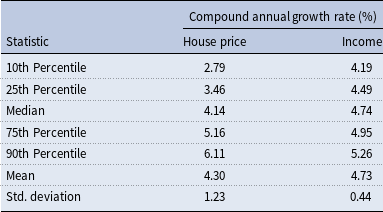
To obtain balanced data without missing house price index and control variables, we are left with 375 MSAs in our dataset. Table 1 provides summary statistics for nominal house price growth rates and nominal income growth rates. We observe that house price growth rates exhibit greater geographical variation compared to income growth rates, despite having similar averages. Therefore, housing price dynamics are influenced by regional factors other than income, which are worthy of exploration, particularly under the scenario of monetary policy shocks.

Table 1.

Summary statistics: house price and income growth

Table 1. Long description

A table comparing house price and income growth rates across percentiles and mean values. The table has 8 rows and 3 columns. The columns are labeled ‘Statistic’, ‘House price’, and ‘Income’. The rows are labeled with percentiles (10th, 25th, Median, 75th, 90th), Mean, and Std. deviation. Row 1: 10th Percentile, 2.79, 4.19. Row 2: 25th Percentile, 3.46, 4.49. Row 3: Median, 4.14, 4.74. Row 4: 75th Percentile, 5.16, 4.95. Row 5: 90th Percentile, 6.11, 5.26. Row 6: Mean, 4.30, 4.73. Row 7: Std. deviation, 1.23, 0.44. The table shows that house price growth rates exhibit greater geographical variation compared to income growth rates, despite having similar averages.

Notes: This table reports summary statistics for the compound annual growth rates of nominal house prices and nominal personal income per capita across 375 metropolitan statistical areas (MSAs) from January 1983 to December 2007.

3.2 Baseline specification

We are interested in estimating the dynamic response of house prices to monetary policy shocks. To achieve this, we estimate the cumulative percentage responses of house prices $h$ months after a monetary policy shock, for $h=1, 2, \ldots , 60$ . The advantage of this method is that local projections allow for nonlinear effects of monetary policy, which provides a convenient baseline framework to explore the heterogeneity of monetary policy impacts between areas of high and low urban growth.Footnote ⁷

We begin with a reduced-form specification without considering heterogeneity between urban growth rate:

(13) \begin{equation} y_{i,t+h} - y_{i,t} = \alpha _{i} + \beta ^h_o RR_t + \phi ' x_{i,t} + \epsilon _{i}. \end{equation}

where $y_{i,t+h} - y_{i,t}$ is the cumulative change in house price from $t$ to $t+h$ in MSA $i$ . $RR_t$ is the Romer-Romer shock. The coefficient $\beta ^h_o$ captures the cumulative house price response to a monetary policy shock $h$ months after the shock happens. $\alpha _i$ denotes the MSA fixed effect, which controls for MSA-specific long-term trends and other time-invariant characteristics. The control variables $x_{i,t}$ include the 1-month to 12-month lagged changes in house prices, the log change of personal income per capita, the level of working-age population (aged 15–64 years), and the branching deregulation index.Footnote ⁸

We estimate the model using Conley (Reference Conley1999) standard errors, which are robust to both spatial correlation and autocorrelation.Footnote ⁹ We set a threshold of 100 miles for the spatial correlation, which allows for spatial correlation of an MSA and other ones located within a radius of 100 miles from its centroid. Following Aastveit and Anundsen (Reference Aastveit and Anundsen2022), we use a kernel that decays linearly with distance in all directions to account for spatial correlation.

To investigate the heterogeneous effects of monetary policy across areas with different urban growth, we further include the interaction of high urban growth and the monetary policy shocks. Specifically, we estimate:

(14) \begin{equation} y_{i,t+h} - y_{i,t} = \alpha _{i} + \beta ^h RR_t + \tilde {\beta }^h RR_t \times I_{i} + \phi ' x_{i,t} + \epsilon _{i}. \end{equation}

where $I_{i}$ is a dummy variable indicating high urban growth. For the control variables, we also interact them with the high urban growth dummy. We do not need to include the urban growth dummy $I_{i}$ in the regression, since it is already absorbed by the MSA fixed effect.

The parameters of interest are $\beta ^h$ and $\tilde {\beta }^h$ , where $\beta ^h$ captures the baseline cumulative house price response to a monetary policy shock $h$ months after the shock happens in low urban growth areas, and $\tilde {\beta }^h$ captures the additional monetary policy effects in high urban growth areas. We are mainly interested in whether $\tilde {\beta }^h$ is statistically significant and the explanation for the possible heterogeneity between high and low urban growth areas.

3.3 Results

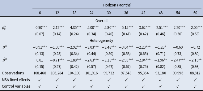
Table 2 shows the cumulative responses of house prices to a monetary policy shock at selected horizons over all the 375 MSAs. We first present the overall effect of monetary policy shock on housing prices using the estimated $\beta ^h_o$ in equation (13), shown in row (1). Rows (2) and (3) present the estimated coefficients $\beta ^h$ and $\tilde {\beta }^h$ in equation (14), respectively, which demonstrate the possible heterogeneity between areas of different urban growth. For the sake of brevity, we report the estimated coefficients every half year.

Table 2.

Response of house prices to a monetary shock and heterogeneity in high growth MSAs

Table 2. Long description

The table presents the cumulative responses of house prices to a monetary policy shock at selected horizons over all 375 MSAs. It includes data for horizons ranging from 6 to 60 months. The table is divided into three main rows: Overall, Heterogeneity, and Observations. Each row contains values for each horizon. The Overall row shows the overall effect of monetary policy shock on housing prices. The Heterogeneity row demonstrates the possible heterogeneity between areas of different urban growth. The Observations row lists the number of observations for each horizon. Standard errors are shown in parentheses. The table also includes information on MSA fixed effects and control variables.

Notes: This table presents results based on two specifications: the overall effect of monetary policy shocks on house prices based on equation (13), and the heterogeneous effects across low- and high-urban-growth areas based on equation (14). Standard errors are shown in parentheses. * $p\lt 0.10$ , ** $p\lt 0.05$ , *** $p\lt 0.01$ .

Overall, without considering the heterogeneity between low urban growth and high urban growth MSAs, the real house prices increase by approximately 5.0% two years after a one percentage point reduction in the policy interest rate. Williams (Reference Williams2015) provide an overview of the literature estimating the cumulative response of house prices to monetary policy shocks, summarizing a response range from 1.7% to 10.4% after two years. Our result falls within this range.

Based on rows (2) and (3), apart from the early 6 month horizon, we find house prices in high urban growth areas are more responsive to monetary policy shocks compared to areas experiencing low urban growth. In high urban growth MSAs, house prices increase by an additional 2.63% two years after an easing monetary shock, compared to the baseline 3.03% housing price increase in low urban growth MSAs. Figure 1 displays the impulse response of house prices across high and low urban growth MSAs separately. The shaded areas are the 95% error bands for the responses. The deepest response occurs 30 months after a monetary shock. A one percentage point reduction in policy interest rates leads to a 3.48% increase in house prices in low urban growth areas and a 6.63% increase in high urban growth areas after two and a half years. The amplified response of the high urban growth MSAs, as represented by the negative $\tilde {\beta }^{h}$ , becomes significant starting in the 9-month horizon, and persists to the 60-month horizon.

Figure 1.

Cumulative response of house prices to a monetary policy shock.

Notes: The blue line represents the cumulative change of house prices responding to a monetary policy shock in high urban growth metro areas, and the red line is in low urban growth metro areas. Shaded area: two standard deviation pointwise confidence bands using spatial correlation robust standard errors.

3.4 Robustness and sensitivity checks

Alternative classifications of high and low urban growth: In our baseline specification, we classify MSAs based on the 25th percentile of cumulative population growth rate across all MSAs from 1983 to 2007. For sensitivity checks, we use different cutoffs for classification, including a 0% population growth rate and the 50th percentile. Though the subsample of MSAs experiencing population loss during 1983–2007 is small, the heterogeneity between areas with different urban growth using the 0% population growth rate cutoff is still evident, as presented in Appendix Table A1.Footnote ¹⁰ Appendix Table A2 similarly shows that our empirical findings remain robust using the 50th percentile cutoff.

In addition, we conduct an alternative classification using the past 10-year population growth rates, instead of the cumulative growth rates over the entire sample period. Specifically, for any given year $T$ , we calculate the cumulative population growth rate between year $T-1$ and year $T-10$ . Then, we obtain the 25th percentile of the past 10-year growth rates. In year $T$ , if an MSA’s past 10-year growth rate exceeds the 25th percentile, it is classified as belonging to the high urban growth category in year $T$ . As illustrated in Section 3.1, the trends of urban growth and decline are largely persistent. If a metro area was growing in the past 10 years, it is likely to continue growing in the future 10 years. This persistence supports the use of past 10-year local trends to categorize urban growth and decline for sensitivity checks. The results stored in Table A3 demonstrate evident heterogeneity of monetary policy impacts between high and low urban growth MSAs using the past 10-year growth rate cutoff.

Longer sample periods and alternative identification of monetary policy shocks: In the baseline specifications (13) and (14), we use Romer-Romer series extended by Wieland and Yang (Reference Wieland and Yang2020) for monetary policy shocks, which ends in 2007. To investigate whether our results are sensitive to a particular sample period, we first construct an extended Romer-Romer shock series that ends in 2019:12 using the same methodology of Romer and Romer (Reference Romer and Romer2004). To address the lack of federal fund rate movement during the zero lower bound period, we use the Wu-Xia shadow rate constructed by Wu and Xia (Reference Wu and Xia2016) to replace the federal fund rate originally used in Romer and Romer (Reference Romer and Romer2004) and Wieland and Yang (Reference Wieland and Yang2020).Footnote ¹¹ When using the updated sample that ends in 2019, we exclude the 2008:01–2009:06 crisis period with excess financial turbulence. Table A4 reports the estimation results based on equation (14) with the extended sample, and demonstrates that the heterogeneity of monetary policy impacts between high and low urban growth MSAs remains robust.

To mitigate concerns that Romer-Romer series are associated with other macro fluctuations, we also utilize high-frequency monetary surprises from Miranda-Agrippino and Ricco (Reference Miranda-Agrippino and Ricco2021) as an instrumental variable for monetary policy shocks.Footnote ¹² The high frequency instrument controls for the “information effect” in the central bank’s monetary policy adjustment. We choose the Wu-Xia shadow rate as our policy variable, and use the high-frequency monetary surprises as instrument. The results in Table A5 show that our results are robust to alternative identifications of monetary policy shocks.

Controlling for regional economic shocks: To control for regional economic shocks such as housing boom-bust cycles, we further include division-by-year fixed effects.Footnote ¹³ The results reported in Table A6 show that our results are robust to controlling for regional economic shocks.

4.1 Data for land scarcity

To measure the land scarcity suggested by equation (10), we calculate $N_0 / N$ , which represents the fraction of developed land $N_0$ over the total developable land $N$ . First, we need to determine the total area of developable land, defined as the land available for residential or commercial real estate development, according to Saiz (Reference Saiz2010). Utilizing elevation data from the USGS (United States Geological Survey) Digital Elevation Model (DEM), we exclude areas with a slope above 15 degrees, as such slopes pose severe constraints for residential construction according to architectural guidelines. For instance, as depicted in Figure 2, the Los Angeles–Long Beach–Anaheim metropolitan area exhibits steep slopes that are not suitable for residential construction, as evident by the vast area in black.

Next, we exclude water bodies, herbaceous wetlands, woody wetlands, and areas covered in snow from the flat terrain. The remaining flat land is considered developable. To achieve this, we utilize a recently published dataset on land cover in the continental United States from the Annual NLCD.Footnote ¹⁴ This database provides raster data with a resolution of 30 m $\times$ 30 m, measuring land use in the U.S. for each year from 1985 to 2024. It was developed by the USGS and includes 16 types of land cover (with a 17th type representing steep slopes additionally derived from the USGS DEM), as shown in the legend in Figure 2.

Figure 2.

Land cover in Los Angeles–Long beach–Anaheim MSA.

Notes: The figure displays the 1985 and 2007 land cover in the Los Angeles–Long beach–Anaheim metropolitan area.

Second, we measure the area of developed land that are of different development intensity, all categorized as “Developed” on the map. The developed area expands over time. By comparing panels (a) and (b) in Figure 2, we observe urban sprawl in the southern part of the Los Angeles–Long Beach–Anaheim MSA (Orange County), consistent with its prosperity in tourism and electronics industries after the 1980s. In addition, land development in the adjacent Riverside–San Bernardino–Ontario MSA (on the right-hand side of Greater Los Angeles) is also notable, indicating the co-development of several metropolitan areas in Southern California.

Land development intensity can vary within urban areas. While Downtown Los Angeles contains a dense concentration of banks, entertainment centers, and other commercial facilities, the San Fernando Valley is less dense, consisting of residential communities and urban parks. This variation is reflected in the Annual NLCD database legend, which categorizes developed areas into four types, as indicated in Figure 2: Developed, Open Space; Developed, Low Intensity; Developed, Medium Intensity; Developed, High Intensity.

According to the documentation of the Annual NLCD, open space refers to areas with a mixture of some constructed materials but mostly vegetation, such as lawn grasses. Impervious surfaces account for less than 20% of total cover, where the fraction of imperviousness is defined as the percentage of a 30-meter pixel covered by artificial substrates or structures (pavement, concrete, rooftops, and other constructed materials) that are assumed to be impermeable to water. In contrast, high intensity refers to highly developed areas with dense human activity, including apartment complexes, row houses, and commercial or industrial zones, where impervious surfaces account for 80% to 100% of total cover. For low- and medium-intensity areas, impervious surfaces account for 20%–49% and 50%–79% of total cover, respectively.

Besides the four categories (Developed, Open Space; Developed, Low Intensity; Developed, Medium Intensity; Developed, High Intensity), the Annual NLCD directly provides the fraction of imperviousness with integer percentages ranging from 0% to 100%, as show in Figure A1. The black areas are undeveloped area with 0% imperviousness. The magenta color areas represent developed areas, with the saturation of the color illustrating the percentage of imperviousness.

Following Saiz (Reference Saiz2010), we quantify an MSA’s land scarcity by focusing on a 50 km radius around its central cities. Within this radius, we measure the area of total developable land, denoted as $N$ . This approach is similar to the method used by Saiz (Reference Saiz2010) in constructing housing supply elasticity. Additionally, we measure the total developed area $N_0$ within the same radius by summing all the areas labeled as “Developed,” with weight assigned to each pixel by its fraction of imperviousness. We calculate land scarcity as $N_0 / N$ for each year, obtaining panel data of annual land scarcity across MSAs.

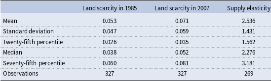
After implementing the aforementioned procedure, we construct panel data on land scarcity for 327 MSAs spanning the period from 1985 to 2007. As Table 3 shows, the average land scarcity was 0.053 in 1985 and increased to 0.071 in 2007, reflecting the urbanization trend in the US over this period. During this period, variations in land scarcity grew larger, as indicated by the standard deviation, which increased from 0.047 to 0.059. While some urban areas experienced remarkable land development between 1985 and 2007, others did not.

The change in land scarcity between 1985 and 2007 is visualized in Figure 3. Los Angeles, New York, and Miami are the top three MSAs with the highest land scarcity. Notably, the increase in land scarcity in Miami was larger than other MSAs, rising from 0.302 to 0.408, equivalent to a 35% increase. In contrast, Pittsburgh and Portland experienced smaller changes in land scarcity.

Table 3.

Summary statistics: land scarcity and saiz supply elasticity

Table 3. Long description

A table with three columns and eight rows comparing land scarcity and supply elasticity statistics across years. The columns are labeled ‘Land scarcity in 1985’, ‘Land scarcity in 2007’, and ‘Supply elasticity’. The rows are labeled with statistical measures: Mean, Standard deviation, Twenty-fifth percentile, Median, Seventy-fifth percentile, and Observations. Row 1: Mean, 0.053, 0.071, 2.536. Row 2: Standard deviation, 0.047, 0.059, 1.431. Row 3: Twenty-fifth percentile, 0.026, 0.035, 1.562. Row 4: Median, 0.038, 0.052, 2.276. Row 5: Seventy-fifth percentile, 0.060, 0.081, 3.181. Row 6: Observations, 327, 327, 269.

Notes: The land scarcity measure is constructed by the authors using data from the Annual NLCD, which varies over time. The supply elasticity is the time-invariant Saiz elasticity from Saiz (Reference Saiz2010).

Figure 3.

Land scarcity in 1985 vs 2007.

Notes: This figure compares land scarcity in 1985 and 2007 across MSAs. The sample includes the 20 MSAs with the lowest Saiz housing-supply elasticities among those whose population exceeded one million in 1996—the midpoint of the 1985–2007 period.

4.2 Land scarcity, supply elasticity, and housing supply

As discussed earlier, land scarcity is partially related to the housing supply elasticity estimated by Saiz (Reference Saiz2010). We quantify land scarcity by calculating the fraction of developed land over the total amount of developable land, denoted as $N_0/N$ . The total area of developable land, represented by $N$ , is fixed and determined by topographical conditions such as land slopes. The method we use to measure $N$ is similar to the approach employed by Saiz (Reference Saiz2010) to estimate the amount of developable land in U.S. metropolitan areas and to characterize housing supply elasticities. This establishes the relevance between land scarcity and the Saiz supply elasticity.

However, whether land has been developed also influences housing supply. Building a house in a congested residential area or a compact business district is different from constructing one on spacious pasture land. This paper creatively accounts for the amount of developed land and undeveloped land in an MSA for each year, which are overlooked in the literature. Therefore, land scarcity introduces a novel aspect not considered in the estimation of housing supply elasticity by Saiz (Reference Saiz2010), based on the recently published land cover database, and it may complement supply elasticity with additional geographic information.

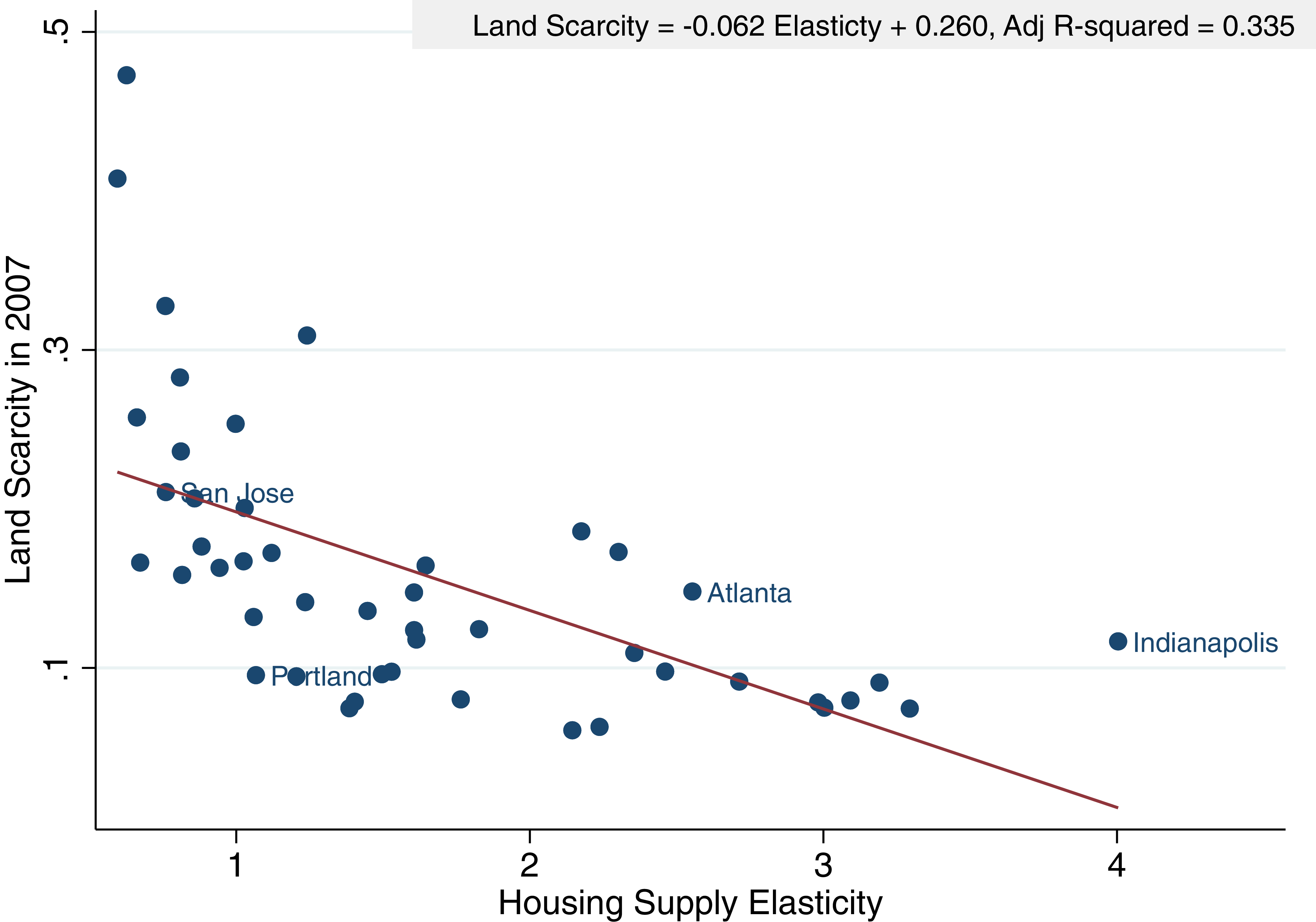
Figure 4 illustrates a scatter plot of land scarcity in 2007 and housing supply elasticity for 47 MSAs with population greater than one million in 1996, the midpoint of 1985 and 2007. Land scarcity shows a negative correlation with supply elasticity, as expected. When the total amount of developable land $N$ is larger, land is less constrained, thus housing supply is more elastic and undeveloped land is less scarce. Mathematically, land scarcity, represented by $N_0/N$ , is lower when $N$ is larger. A simple linear regression confirms this relationship, with the coefficient of supply elasticity being $-0.062$ and the corresponding p-value being lower than 0.001. The $R^2$ is $0.335$ , indicating partial relevance between land scarcity and housing supply elasticity.

Figure 4.

Land scarcity and supply elasticity.

In addition, in Figure 4, we observe that some MSAs may have similar housing supply elasticities but differ in levels of land scarcity. For instance, both San Jose and Portland are coastal metropolitan areas in the West region; however, land scarcity in San Jose is notably larger than in Portland. Furthermore, some MSAs have higher supply elasticities but higher levels of land scarcity than Portland, as seen in examples such as Atlanta and Indianapolis. This is conceivable because the substantial amount of developable land in these flat metropolitan areas may be widely utilized for purposes such as transportation or serving as a state capital. These examples suggest that land scarcity may provide additional information about the local land or housing market supply that are not captured by supply elasticity alone.

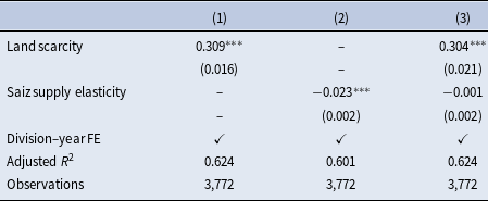
Second, we can investigate whether land scarcity contributes to the housing supply in local markets. The scarcity of land has a direct influence on its value. When undeveloped land is more scarce in a metropolitan area, its land value tends to be higher. To examine the relationship between the land value and land scarcity, we obtain quarterly land value data for metro areas from Davis and Palumbo (Reference Davis and Palumbo2008) and perform a panel regression across the years 1985–2007, controlling the division-year fixed effects. The results, shown in Table 4 column (1), confirm a significantly positive association between land scarcity and land value.

Table 4 column (2) indicates a lower adjusted $R^2$ compared to column (1), suggesting that land scarcity demonstrates a greater explanatory power for land value compared to housing supply elasticity. In column (3), we include both land scarcity and housing supply elasticity as explanatory variables and conduct a likelihood ratio test comparing the nested models of columns (2) and (3). The test statistic is 221.95 and the associated p-value is lower than 0.0001, supporting the inclusion of land scarcity. In contrast, when comparing the nested models of columns (1) and (3), the test statistic is 0.20, with a higher p-value of 0.6529.

Land scarcity might influence house prices through its impact on land value. As outlined by Glaeser and Gyourko (Reference Glaeser and Gyourko2018), house prices $P$ are comprised of several components, including land cost, physical construction costs, and entrepreneurial profits to compensate home builders. They estimate the “minimum profitable production cost” ( $MPPC$ ) based on RSMeans Company data, covering physical construction costs such as materials, labor, and equipment, but not land costs. Therefore, the combination of land cost and profit is reflected in the price after deducting the construction costs, which is the $P-MPPC$ component. Notably, Glaeser and Gyourko (Reference Glaeser and Gyourko2018) observe that construction costs ( $MPPC$ ) have not risen much over time. This implies that when land cost rises along with increasing land scarcity, it might lead to higher $P/MPPC$ . Based on the biannual data for the median $P/MPPC$ provided by Glaeser and Gyourko (Reference Glaeser and Gyourko2018), we explore the relationship between land scarcity and $P/MPPC$ . 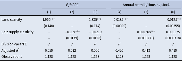Similar to land value, we utilize on the $P/MPPC$ information for each MSA provided by Glaeser and Gyourko (Reference Glaeser and Gyourko2018) over the period of 1985–2007 and conduct a panel regression. Table 5 column (1) confirms the positive association between land scarcity and $P/MPPC$ . Estimation results with housing supply elasticity in column (2) indicates a lower adjusted $R^2$ compared to column (1). The likelihood ratio test comparing columns (2) and (3) results in a high test statistic (116.70) with an p-value lower than 0.0001. In contrast, the comparison between columns (1) and (3) yields a lower test statistic (2.18) and a high p-value (0.1397).

Table 4.

Land scarcity, supply elasticity, and land value

Table 4. Long description

A table with three columns and four rows, including a header row. The columns are labeled (1), (2), and (3). The row labels are Land scarcity, Saiz supply elasticity, Division-year FE, Adjusted R squared, and Observations. Row 1: Land scarcity, 0.309***, 0.304***; Row 2: Saiz supply elasticity, -0.023***, -0.001; Row 3: Division-year FE, checked, checked; Row 4: Adjusted R squared, 0.624, 0.601, 0.624; Row 5: Observations, 3,772, 3,772, 3,772. The table presents statistical data on the relationship between land scarcity, supply elasticity, and land value, with significant values marked by asterisks.

Notes: The dependent variable is the land value. Land value data are from Davis and Palumbo (Reference Davis and Palumbo2008). Standard errors are shown in parentheses. * $p\lt 0.10$ , ** $p\lt 0.05$ , *** $p\lt 0.01$ .

Table 5.

Land scarcity, supply elasticity, price-to-cost ratio, and permit activity

Table 5. Long description

A table with six columns and six rows, including a header row. The columns are labeled as follows: (1) Land scarcity, (2) Saiz supply elasticity, (3) Division-year fixed effects, (4) Annual permits/Housing stock, (5) Adjusted R-squared, and (6) Observations. The rows present statistical data with values and standard errors in parentheses. Row 1: Land scarcity shows values 1.965, 1.835, -0.0135, and -0.0125 with standard errors 0.148, 0.174, 0.00300, and 0.00355. Row 2: Saiz supply elasticity shows values -0.109, -0.0219, 0.000768, and 0.000175 with standard errors 0.0139, 0.0156, 0.000271, and 0.000318. Row 3: Division-year fixed effects are marked with checkmarks. Row 4: Adjusted R-squared values are 0.559, 0.512, 0.560, 0.420, 0.413, and 0.419. Row 5: Observations are consistently 1128 across all columns.

Notes: Columns (1)–(3) report results for the price-to-construction-cost ratio ( $P/MPPC$ ). Columns (4)–(6) report results for the annual permit rate (permits issued divided by the housing stock in 2000). Standard errors are shown in parentheses. * $p\lt 0.10$ , ** $p\lt 0.05$ , *** $p\lt 0.01$ .

The patterns for housing permits are similar. In an area where undeveloped land is more scarce, the constraint on housing supply should be reflected by lower housing permits issuance rate. Therefore, we also examine whether housing permit issuance rate, represented by annual number of housing permits issued divided by total housing stock in 2000, also provided by Glaeser and Gyourko (Reference Glaeser and Gyourko2018), is related to land scarcity. As expected, Table 5 confirms that land scarcity and permit issuance rate are negatively related. The likelihood ratio test comparing columns (5) and (6) results in a high test statistic (13.62) with a low p-value (0.0002). In contrast, the comparison between columns (4) and (6) yields a test statistic 0.34 and a high p-value 0.5613.Footnote ¹⁵

As argued by Glaeser and Gyourko (Reference Glaeser and Gyourko2018), the shape and the slope of the housing supply curve are associated with the value of $P/MPPC$ . High land scarcity corresponds to higher land value and higher $P/MPPC$ , as well as lower issuance rate of housing permits, which may indicate a steeper slope of the housing supply curve. Therefore, land scarcity might contribute to house price dynamics, especially in response to monetary policy shocks.

4.3 Heterogeneous effects of monetary policy shocks and land scarcity

We have confirmed that land scarcity contributes to housing supply. In the next step, we test the hypothesis in Section 2 that monetary policy effects are determined by the interaction of population growth rate $N_1 / N_0$ and land scarcity $N_0 / N$ . Equation (10) and Proposition1 together suggest the following two conjectures.

Conjecture 1: In areas with abundant undeveloped land, the heterogeneity of monetary policy effects across high and low urban growth MSAs is muted.

Conjecture 2: The effects of monetary policy in high urban growth areas are stronger when undeveloped land is more scarce.

In areas with scarce undeveloped land ( $N_0 / N$ is large), home builders expect that population growth will further intensify land shortage in the future. Therefore, the impacts of monetary policy shocks are determined by the interaction of urban growth and land scarcity. In areas with high urban growth combined with large land scarcity, which relates to $\mu \gt 1$ in our Section 2 model, the prospect of future land shortage leads to a larger monetary policy response, as proposed by Conjecture 2. In contrast, in areas with abundant undeveloped land ( $N_0 / N$ is small), land is not likely to be depleted in the next several years when the population grows. Therefore, Conjecture 1 proposes that the heterogeneity of monetary policy effects between high and low urban growth MSAs is expected to be insignificant.

To test both conjectures, in equation (15) we augment the baseline specification by interacting with land scarcity. $LandScarcity_{i,t}$ denotes the land scarcity for MSA $i$ in a certain year-month $t$ . We standardize land scarcity by scaling it with its standard deviation.

(15) \begin{align} y_{i,t+h} - y_{i,t} & = \alpha _{i} + \beta ^h RR_t +\tilde {\beta }^h RR_t \times I_{i} + \tilde {\beta }_{LS}^h RR_t \times LandScarcity_{i,t}\nonumber \\ &\quad + \tilde {\beta }_{HLS}^h RR_t \times I_{i} \times LandScarcity_{i,t} + \phi ' x_{i,t} +\epsilon _{i,t}. \end{align}

In the augmented specification, the introduction of land scarcity into the regression changes the interpretation of $\beta ^h$ and $\tilde {\beta }^h$ , compared to the baseline regression in equation (14). Both coefficients represent the housing price response to a monetary policy shock in an MSA with minimal land scarcity, with $\tilde {\beta }^h$ showing the additional effect of high urban growth. 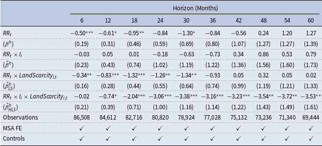Therefore, Conjecture 1 can be verified with the significance of $\tilde {\beta }^h$ , as the coefficient represents the heterogeneity of monetary policy effects in an area with abundant undeveloped land. As demonstrated in Table 6, $\tilde {\beta }^h$ are insignificant across different horizons, demonstrating the muted housing price response to monetary policy in an area with abundant undeveloped land, regardless of population growth.

Table 6.

Heterogeneous effects of MP shocks, augmented with land scarcity

Table 6. Long description

The table presents cumulative responses of house prices to a monetary policy shock over various horizons, estimated based on equation (15). It includes standard errors in parentheses and significance levels denoted by asterisks. The table has 10 columns representing different horizons in months (6, 12, 18, 24, 30, 36, 42, 48, 54, 60) and 5 rows of data with labels (β^R), (β^R_i), (β^LS), (β^LS_i), and (β^LS_i). Each cell contains numerical values and standard errors. The table also includes the number of observations for each horizon and indicates the inclusion of MSA fixed effects and controls.

Notes: This table reports cumulative responses of house prices to a monetary policy shock ( $RR_t$ ) over different horizons, estimated based on equation (15). Standard errors are shown in parentheses. * $p\lt 0.10$ , ** $p\lt 0.05$ , *** $p\lt 0.01$ .

To test Conjecture 2, we revisit the estimation in equation (15) and focus on the triple interaction coefficient $\tilde {\beta }_{HLS}^h$ . If Conjecture 2 is valid, then we expect $\tilde {\beta }_{HLS}^h$ to exhibit a significant negative value, demonstrating that land scarcity and high urban growth reinforce each other in generating a large monetary policy effect on housing prices. Table 6 confirms that the coefficient $\tilde {\beta }^h_{HLS}$ is indeed both significant and negative across most of the horizons. This result indicates that the effect of monetary policy in high urban growth MSAs is stronger when undeveloped land is more scarce, confirming Conjecture 2.Footnote ¹⁶

In Section 4.2, we find that land scarcity and the Saiz supply elasticity are negatively correlated, and that both measures contain meaningful information for explaining regional housing supply. A natural follow-up question is whether the Saiz elasticity can also explain heterogeneity in monetary policy effects stemming from urban growth. We estimate a specification similar to equation (15), but replace land scarcity with the Saiz supply elasticity:

(16) \begin{align} y_{i,t+h} - y_{i,t} & = \alpha _{i} + \beta ^h RR_t +\tilde {\beta }^h RR_t \times I_{i} + \tilde {\beta }_{ELA}^h RR_t \times (1/Elasticity_{i,t})\nonumber \\&\quad + \tilde {\beta }_{HELA}^h RR_t \times I_{i} \times (1/Elasticity_{i}) + \phi ' x_{i} +\epsilon _{i,t}. \end{align}

For the sake of clarity, the coefficients on the interaction terms that includes the Saiz elasticity variable $Elasticity_{i}$ is labeled with $ELA$ instead of $LS$ . We drop the time $t$ in the subscript, as Saiz elasticity does not change over time. Since Saiz elasticity broadly measures the total developable land, it reflects the value of $N$ shown in our model. A larger $N$ naturally relates to more developable land and a larger land supply elasticity $Elasticity_{i}$ . Accordingly, this generates the negative correlation with land scarcity shown in Figure 4, as land scarcity represents $\frac {N_0}{N}$ . 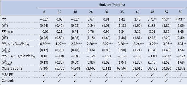To facilitate a similar interpretation to Table 6, therefore, we use the inverse of Saiz elasticity $1/Elasticity_{i}$ in equation (16) and expect $\tilde {\beta }_{HELA}^h$ , the coefficients of the interaction term $RR_t \times I_{i} \times (1/Elasticity_{i})$ to be negative. As expected, the fourth row in Table 7 displays negative coefficients, though not significant. The third row displays negative estimates for the coefficients of $RR_t \times (1/Elasticity_{i})$ , in line with Aastveit and Anundsen (Reference Aastveit and Anundsen2022) that less elastic areas see greater impacts on housing prices following a monetary policy shock. This demonstrates that Saiz elasticity by itself generate heterogeneous monetary policy effects across MSAs, while land scarcity helps to explain the heterogeneous monetary policy effects related with cross-MSA urban growth differences.

Table 7.

Heterogeneous effects of MP shocks, augmented with supply elasticity

Table 7. Long description

The table presents cumulative responses of house prices to a monetary policy shock over various horizons, measured in months. It includes data for horizons ranging from 6 to 60 months. The table has 10 columns representing different horizons and 7 rows representing different variables and their standard errors. The variables include RR, RRi, RRi x 1/Elasticity, and RRi x 1/Elasticityi, with standard errors shown in parentheses. The table also lists the number of observations for each horizon and indicates the inclusion of MSA fixed effects and controls. Notable trends include the increasing values of RR and RRi over time, with standard errors also increasing. The interaction terms involving elasticity show varying patterns across different horizons.

Notes: This table reports cumulative responses of house prices to a monetary policy shock ( $RR_t$ ) over different horizons, estimated based on equation (16). Standard errors are shown in parentheses. * $p\lt 0.10$ , ** $p\lt 0.05$ , *** $p\lt 0.01$ .

We also examine if there may be alternative mechanisms beyond land supply that affect the pass through of monetary policy shocks to housing prices. Scharfstein and Sunderam (Reference Scharfstein and Sunderam2016) show that high concentration in mortgage lending reduces the sensitivity of mortgage rates and refinancing activity to mortgage-backed security yields. Therefore, if areas with high urban growth are also places in which market power of mortgage lending is small, then larger pass-through of monetary shocks to lending cost would also generate the larger response in housing price responses following a monetary policy shock in high urban growth areas. We similarly check if demographic pattern may affect the housing price response via the differential housing purchasing patterns among different age groups. As documented in Francke and Korevaar (Reference Francke and Korevaar2025), individuals are more likely to be housing buyers when they are young. Therefore, regional heterogeneity in young cohort size may also affects the responsiveness of housing price to monetary policy shocks.

To control for market concentration and demographic pattern, we augment equation (15) by introducing the bank concentration variable $HHI_{i,t}$ or the share of young adults $Youngshare_{i,t}$ into the regression.Footnote ¹⁷ Specifically, we interact the terms reported in Table 6 with $HHI_{i,t}$ or $Youngshare_{i,t}$ directly. This allows us to determine whether the conjectures hold for MSAs with a certain value of $HHI_{i,t}$ or $Youngshare_{i,t}$ . For the sake of clarity and ease in comparison across tables, we set $HHI_{i,t}$ or $Youngshare_{i,t}$ at its low level of 25th percentile, and its high level of 75th percentile, respectively. We report the coefficients shown in Table 6 augmented with high or low $HHI_{i,t}$ (or $Youngshare_{i,t}$ ) at the corresponding percentile. Tables A9 and A10 in the appendix report the results for $HHI_{i,t}$ , while Tables A11 and A12 report the results for $Youngshare_{i,t}$ , respectively. For bank concentration, Conjecture 1 holds well in both tables, and Conjecture 2 is more evident when bank HHI is low. This likely reflects that less competitive mortgage lending markets reduces the responsiveness of monetary policy pass-through, thus counteracting the amplification from the interaction between land scarcity and urban growth. As for $Youngshare_{i,t}$ , we observe that Conjecture 2 is verified in both Tables A11 and A12. Interestingly, we observe that high urban growth in land abundant regions display relatively large monetary response when the share of young people is low. This likely reflects areas with attractive amenity for elderly, which attract retiree migrants with housing demand.

4.4 MSA-by-MSA analysis

In addition to exploring the estimated effects of monetary policy shocks across MSAs, we examine the MSA-specific estimates in this subsection. This MSA-by-MSA analysis allows us to regard each metropolitan area as an individual housing market. Therefore, we can investigate if the MSA-specific monetary policy effects on house prices are determined by local characteristics, specifically urban growth and land scarcity together.

To obtain the MSA-specific estimates for the impacts of monetary policy shocks on house prices, we perform local projections MSA-by-MSA instead of panel regressions, with the MSA-by-MSA regression specification closely aligning with our baseline model. The main difference is that we utilize data for each MSA during the period of 1983–2007 to obtain the MSA-specific estimate. For each MSA $m$ , we perform the following regressions:

\begin{align*} y_{m,t+h} - y_{m,t} = \alpha _m + \beta _m^h \epsilon _t + \phi ' x_{m,t} + u_{m,t+h}, \end{align*}

where $y_{m,t+h} - y_{m,t}$ is the cumulative house price growth rate from $t$ to $t+h$ , and $\beta ^h_m$ captures the cumulative house price response in MSA $m$ to a monetary policy shock $h$ months after the shock happens. $\epsilon _t$ is the monetary policy shock. The parameter $\alpha _m$ is the MSA-specific intercept.

We collect the deepest (largest in absolute value) cumulative house price responses within five years for each MSA, i.e. $\beta _m = max\{ |\beta _m^h | \}$ . Among the 375 MSA-specific deepest cumulative responses, the median level is 4.26% and the mean value is 5.73%, which is consistent with the deepest cumulative response of 5.80% at the 30 months horizon in Table 2. If an MSA-specific deepest cumulative response $\beta _m$ is above the median level 4.26%, we consider it as indicating large monetary policy impacts on house prices in MSA $m$ . Conversely, if $\beta _m$ falls below 4.26%, we interpret it as suggesting smaller impacts.

We use a scatter plot in Figure 5 panel (a) to illustrate MSA-specific monetary policy effects. Each dot, representing an MSA, is marked in blue for large monetary policy effects and in red for small monetary policy effects. To investigate the potential influence of urban growth and local land scarcity on MSA-specific monetary policy impacts on house prices, we specify the scatter plot axes. The cumulative population growth rate is represented on the x-axis, while the average land scarcity during 1985–2007 is depicted on the y-axis.

Figure 5.

MSA-specific estimates.

For MSAs with low population growth rates and low levels of land scarcity, the monetary policy effects are not amplified by the interaction between land scarcity and high urban growth demonstrated in Table 6. According to equation (10) and Proposition1, it is apparent that when monetary policy impacts on house prices are not substantial, the condition $\mu = (N_0/N) \times (N_1/N_0) \leq 1$ is likely to be satisfied. This condition implies that the population growth rate $N_1/N_0$ and land scarcity $N_0/N$ are likely to be low at the same time. Therefore, equation 10 and Proposition1 in Section 2 suggest a third conjecture:

Conjecture 3: MSAs with small monetary policy impacts on house prices tend to exhibit low population growth rates and abundant undeveloped land.

Figure 5 confirms Conjecture 3. In panel (a) of Figure 5, it is evident that nearly all the red dots, representing small monetary policy effects, are situated in an area where both land scarcity and cumulative population growth rate are lower than the corresponding 75th percentile.

To further investigate the role of housing supply elasticity in shaping monetary policy impacts, we present a scatter plot with the y-axis representing standardized Saiz supply elasticity in Figure 5, panel (b). The graph does not demonstrate an obvious pattern regarding the interaction of urban growth and housing supply elasticity.

We acknowledge that the MSA-specific point estimates may not be very accurate. It is possible that the standard errors of MSA-specific point estimates exhibit variation across metropolitan areas. To illustrate, consider two MSAs: one with substantial monetary policy impacts and a large standard deviation, and another with smaller impacts and a smaller standard deviation. In such cases, the first MSA’s lower bound of monetary policy impacts may appear smaller than the other one.

For robustness checks, we validate the pattern observed in Figure 5 panel (a) by examining the lower and upper bounds of 90% confidence intervals for the MSA-specific estimates in Figures A2 and A3. It is evident that the patterns remain consistent, whether plotting the scatter plot with the point estimates or both the lower and the upper bounds of the estimates.