1. Introduction
It was observed by Quincke (Reference Quincke1896) that solid dielectric particles suspended in a slightly conducting liquid and exposed to a sufficiently strong uniform electric field undergo a spontaneous rotation, provided that charge relaxation within the suspending liquid is faster than in the particles. These Quincke rotations are involved in a wide variety of physical phenomena including the occurrence of deterministic chaos in particle motions (Lemaire & Lobry Reference Lemaire and Lobry2002; Peters, Lobry & Lemaire Reference Peters, Lobry and Lemaire2005; Salipante & Vlahovska Reference Salipante and Vlahovska2013), interactions between rotating bodies (Das & Saintillan Reference Das and Saintillan2013), the appearance of collective motions in large populations of motile particles (Bricard et al. Reference Bricard, Caussin, Desreumaux, Dauchot and Bartolo2013; Yeo, Lushi & Vlahovska Reference Yeo, Lushi and Vlahovska2015), the macroscopic behaviour of ‘colloidal motors’ manifested in the drastic reduction of suspension viscosity (Lobry & Lemaire Reference Lobry and Lemaire1999; Cēbers Reference Cēbers2004; Pannacci, Lemaire & Lobry Reference Pannacci, Lemaire and Lobry2007a ; Lemaire et al. Reference Lemaire, Lobry, Pannacci and Peters2008) and the increased conductivity resulting from the introduction of insulating particles (Pannacci, Lobry & Lemaire Reference Pannacci, Lobry and Lemaire2007b ).
Melcher & Taylor (Reference Melcher and Taylor1969) rationalized the Quincke rotation of solid cylindrical ‘rotors’ in terms of their electrohydrodynamic model incorporating surface-charge convection (the rotation of solid spheres was addressed by Jones (Reference Jones1984)) and predicted that drops and bubbles also exhibit a similar effect. Spontaneous rotation of droplets was indeed observed by Krause & Chandratreya (Reference Krause and Chandratreya1998). Following this the phenomenon has been studied experimentally by several groups (Ha & Yang Reference Ha and Yang2000; Salipante & Vlahovska Reference Salipante and Vlahovska2010), the focus being on quantifying the threshold magnitude of the electric field for the onset of rotation.
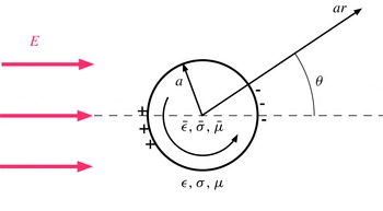
The problem governing drop rotation is inherently three-dimensional (3D) and substantially more complicated than the corresponding problem for a solid particle. As such it seems rather intractable to analysis. To gain insight into the mechanism of spontaneous drop rotation and in view of the reported observation of the rotation of dielectric cylinders (Melcher & Taylor Reference Melcher and Taylor1969) a significant effort has therefore been put into studying the comparable two-dimensional (2D) problem of cylinder rotation. In particular, the simpler case of a solid dielectric rotor has been studied by Melcher & Taylor (Reference Melcher and Taylor1969). When charge relaxation within the suspending liquid is faster than that in the rotor, the surface-charge distribution induced by the applied field has a dipole moment antiparallel to the applied field. For a sufficiently large field magnitude this configuration becomes unstable and rotation occurs; the balance of surface-charge convection and Ohmic charging results in tilting of the induced dipole in a direction giving rise to an electrical torque sustaining the rotation: see figure 1.
Schematic diagram of the 2D rotation of a cylinder in a uniform electric field. The indicated surface-charge distribution corresponds to a faster charge relaxation within the suspending liquid than in the cylinder,
 ${\it\epsilon}/{\it\sigma}<\bar{{\it\epsilon}}/\bar{{\it\sigma}}$
. Counterclockwise rotation convects this distribution; the electric torque acting on the tilted dipole augments this effect, thus balancing viscous resistance. Clockwise rotation is equally likely.

With the 2D fluid motion accompanying the rigid-body rotation of the rotor being a simple potential vortex, the calculation of the rotation speed reduces to the solution of a nonlinear algebraic equation. The comparable rotation of a liquid cylinder is significantly more complicated. This problem was studied for the first time by Feng (Reference Feng2002) using eigenfunction expansions whose coefficients were determined through the numerical solution of a (truncated) infinite system of nonlinear algebraic equations. As in the rotor problem, Feng (Reference Feng2002) found spontaneous electro-rotation beyond a threshold electric field in systems where charge relaxation within the suspending liquid is faster than that in the cylinder. Feng (Reference Feng2002) also presented an intuitive approximation for the electro-rotation velocity by neglecting charge convection aside from that contributed by the potential-vortex component of the 2D flow (associated with drop ‘rotation’). Unsurprisingly, this approximation works well for highly viscous drops, but is less adequate otherwise (see e.g. figure 4 in Feng (Reference Feng2002)). A somewhat similar approach was applied by He, Salipante & Vlahovska (Reference He, Salipante and Vlahovska2013) in the 3D problem.
Following Melcher & Taylor (Reference Melcher and Taylor1969) and Feng (Reference Feng2002), we focus upon the idealized 2D problem. Our goal is to analyse 2D electro-rotation systematically, avoiding ad hoc approximations (as well as the above-mentioned restriction to highly viscous drops). Our approach is based on the following observation. In the Taylor–Melcher electrohydrodynamic model charge convection is quantified by the electric Reynolds number
 $\mathit{Re}$
. Since the fore–aft-symmetric solution becomes unstable at a critical value of
 $\mathit{Re}$
, it is expected that a large-
 $\mathit{Re}$
analysis would reveal electro-rotation. This is the main thrust of the present contribution. Our contribution goes beyond highlighting the nonlinear mechanism of Quincke rotation; indeed, it appears that the singular limit of large
 $\mathit{Re}$
has so far not been addressed. The scaling to be established in this non-intuitive limit may well be relevant to the analysis of the corresponding 3D problem.
2. Formulation
A cylindrical immiscible ‘drop’ (radius
 $a$
, dielectric permittivity
 $\bar{{\it\epsilon}}$
, conductivity
 $\bar{{\it\sigma}}$
, viscosity
 $\bar{{\it\mu}}$
) is suspended in another liquid (dielectric permittivity
 ${\it\epsilon}$
, electric conductivity
 ${\it\sigma}$
, viscosity
 ${\it\mu}$
) and subjected to a uniform electric field of magnitude
 $E$
. Our goal is to calculate the resulting steady-state flow, assuming that surface tension is strong enough to retain an approximately circular drop cross-section. We normalize electric fields and potentials by
 $E$
and
 $aE$
, respectively, the surface-charge density by
 ${\it\epsilon}E$
and the velocity field by Taylor’s velocity scale
 $$\begin{eqnarray}\mathscr{U}=\frac{{\it\epsilon}aE^{2}}{{\it\mu}}.\end{eqnarray}$$
We employ cylindrical coordinates (
 $r,{\it\theta}$
) with
 $r=0$
at the drop axis and
 ${\it\theta}=0$
in the direction of the applied field, see figure 1. The velocity field in the suspending liquid is
 $\boldsymbol{u}=\hat{\boldsymbol{e}}_{r}u+\hat{\boldsymbol{e}}_{{\it\theta}}v$
, while that in the drop is
 $\bar{\boldsymbol{u}}=\hat{\boldsymbol{e}}_{r}\bar{u}+\hat{\boldsymbol{e}}_{{\it\theta}}\bar{v}$
.
The electric potentials
 ${\it\varphi}$
and
 $\bar{{\it\varphi}}$
are governed by Laplace’s equation, regularity at
 $r=0$
and the approach to the uniformly applied field,
 $$\begin{eqnarray}{\it\varphi}\sim -r\cos {\it\theta}\quad \text{as}~r\rightarrow \infty .\end{eqnarray}$$
At
 $r=1$
they satisfy the continuity condition,
 ${\it\varphi}=\bar{{\it\varphi}}$
, as well as the charging condition
 $$\begin{eqnarray}\frac{\partial {\it\varphi}}{\partial r}-R\frac{\partial \bar{{\it\varphi}}}{\partial r}=\mathit{Re}\frac{\partial }{\partial {\it\theta}}(qv),\end{eqnarray}$$
in which
 $R=\bar{{\it\sigma}}/{\it\sigma}$
. The surface-charge density appearing in (2.3) is provided by the jump in electric displacement,
 $$\begin{eqnarray}q=\frac{1}{S}\frac{\partial \bar{{\it\varphi}}}{\partial r}-\frac{\partial {\it\varphi}}{\partial r},\end{eqnarray}$$
in which
 $S={\it\epsilon}/\bar{{\it\epsilon}}$
. The essential difference from the classical description of Taylor (Reference Taylor1966) is the incorporation in (2.3) of charge convection. This nonlinear mechanism is quantified by the electric Reynolds number (Melcher & Taylor Reference Melcher and Taylor1969),
 $$\begin{eqnarray}\mathit{Re}=\frac{{\it\epsilon}^{2}E^{2}}{{\it\sigma}{\it\mu}},\end{eqnarray}$$
constituting the ratio of the charge-relaxation time
 ${\it\epsilon}/{\it\sigma}$
to the convective time
 $a/\mathscr{U}$
.
The velocity fields
 $\boldsymbol{u}$
and
 $\bar{\boldsymbol{u}}$
are governed by the continuity and Stokes equations. At
 $r=1$
they satisfy the impermeability condition,
 $u=\bar{u}=0$
, the continuity condition (tacitly used in (2.3)),
 $v=\bar{v}$
, and the shear-stress balance,
 $$\begin{eqnarray}\frac{\partial v}{\partial r}-v-\frac{1}{M}\left(\frac{\partial \bar{v}}{\partial r}-\bar{v}\right)=q\frac{\partial {\it\varphi}}{\partial {\it\theta}},\end{eqnarray}$$
in which
 $M={\it\mu}/\bar{{\it\mu}}$
. At
 $r=0$
 $\bar{\boldsymbol{u}}$
is regular, while at large
 $r$
 $\boldsymbol{u}$
decays.
3. Symmetry arguments and vanishing of net charge
Even with incorporation of surface convection, the governing equations and boundary conditions still possess an underlying fore–aft symmetry about the midplane
 ${\it\theta}=\pm {\rm\pi}/2$
similar to that in the classical (3D) problem of Taylor (Reference Taylor1966). This may appear to suggest that, under the reflection
 ${\it\theta}\rightarrow {\rm\pi}-{\it\theta}$
, the solutions transform as
 $$\begin{eqnarray}{\it\varphi}\rightarrow -{\it\varphi},\quad q\rightarrow -q,\quad u\rightarrow u,\quad v\rightarrow -v.\end{eqnarray}$$
However, the inherent nonlinearity in the surface convection mechanism now allows for symmetry breaking, with solutions that are not fore–aft-symmetric. (Given the experimental and numerical evidence for spontaneous rotation, we actually anticipate a solution that is not fore–aft-symmetric at sufficiently large
 $\mathit{Re}$
.) Furthermore, the symmetry of the above nonlinear problem with respect to the direction of the applied field necessitates that the ‘mirror image’ of any solution
 $(\boldsymbol{u},q)$
(where
 $q$
and the velocity components are regarded as functions of
 $r$
and
 ${\it\theta}$
), namely
 $$\begin{eqnarray}\hat{\boldsymbol{e}}_{r}u(r,-{\it\theta})-\hat{\boldsymbol{e}}_{{\it\theta}}v(r,-{\it\theta}),\quad q(r,-{\it\theta}),\end{eqnarray}$$
is also a solution.
Allowing for asymmetric solutions, and noting that the slowest decay rate in 2D Stokes flow (Leal Reference Leal2007) is that associated with an irrotational vortex, the far-field decay of
 $\boldsymbol{u}$
implies
 $$\begin{eqnarray}v\sim \frac{{\it\omega}}{r}\quad \text{as}~r\rightarrow \infty .\end{eqnarray}$$
(For fore–aft-symmetric flows, where
 ${\it\omega}=0$
, the decay rate is faster.) By the above-mentioned mirror-image symmetry, a solution involving drop rotation with angular velocity
 ${\it\omega}$
implies the existence of a solution with angular velocity
 $-{\it\omega}$
.
Furthermore, it is readily seen that the vanishing of the total drop charge,
 $$\begin{eqnarray}\int _{0}^{2{\rm\pi}}q\,\text{d}{\it\theta}=0,\end{eqnarray}$$
which trivially holds for fore–aft-symmetric solutions (see (3.1)), is satisfied in general. Indeed, from Laplace’s equation within the drop domain it follows that the integral of
 $\partial \bar{{\it\varphi}}/\partial r$
vanishes at
 $r=1$
. Integration of (2.3) over the unit circle
 $r=1$
implies the same for the integral of
 $\partial {\it\varphi}/\partial r$
. (Since
 $qv$
is necessarily single-valued on the unit circle, it is evident that the integral of the surface-divergence term on the right-hand side of (2.3) vanishes.) We then get (3.4) from integration of (2.4). Physically, (3.4) may be considered a consequence of the Ohmic nature of leaky-dielectric liquids: the net outward flux of electric field associated with a non-zero total drop charge would be accompanied by a net outward charge flux, which is incompatible with the assumed steadiness.
Given the vanishing of the drop’s net charge and the far-field approach (2.2) to a uniform field, the drop does not experience any net electric force (Yariv Reference Yariv2006). The drop is accordingly force-free. It is not, however, necessarily torque-free.
4. Exact solutions
Following Feng (Reference Feng2002) one can solve the exact 2D problem comprising (2.2)–(2.6) and (3.3) for arbitrary
 $\mathit{Re}$
. Indeed, as the only nonlinearities in this system are introduced in conditions (2.3) and (2.6), the electric potentials and stream functions are provided by the standard eigenfunction expansions for Laplace’s equation and the biharmonic equation, respectively. Substituting these expansions into the exact problem yields the flow field, and, in particular, the angular speed
 ${\it\omega}$
appearing in (3.3). As in Feng (Reference Feng2002), we find a bifurcation from a fore–aft-symmetric solution (with
 ${\it\omega}=0$
) for a sufficiently small
 $\mathit{Re}$
to an asymmetric solution (with non-zero
 ${\it\omega}$
) at a sufficiently large
 $\mathit{Re}$
. Provided that
 $RS<1$
, this trend holds for any combination of
 $R$
,
 $S$
and
 $M$
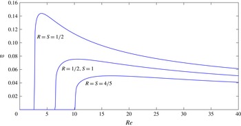
. This bifurcation is illustrated in figure 2, showing the variation of
 ${\it\omega}$
with
 $\mathit{Re}$
for the viscosity ratio
 $M=0.4$
and three sets of liquid pairs represented by the indicated values of
 $R$
and
 $S$
.
Variation with
 $\mathit{Re}$
of the angular velocity
 ${\it\omega}$
, as obtained from an eigenfunction-expansion solution of the exact problem for the indicated values of
 $R$
and
 $S$
. The viscosity ratio is
 $M=0.4$
.

5. Large
 $\mathit{Re}$

Our interest is in the asymptotic limit
 $\mathit{Re}\gg 1$
. Naively, it appears from (2.3) that at leading order
 $qv$
is uniform with
 ${\it\theta}$
at
 $r=1$
; however, constraint (3.4) implies that the continuous field
 $q$
must vanish at some value of
 ${\it\theta}$
, therefore giving the contradictory result
 $qv\equiv 0$
. We therefore need a non-trivial scaling where Ohmic charging balances convection in (2.3).
Because of the far-field approach to a uniform unity field, the gradients of both
 ${\it\varphi}$
and
 $\bar{{\it\varphi}}$
are
 $O(1)$
. This may appear to suggest that
 $q$
is
 $O(1)$
as well. But then (2.3) implies an
 $O(1/\mathit{Re})$
velocity field, whereby (2.6) is unbalanced. This impasse is resolved by noting that even with
 $O(1)$
electric-field distributions, it is possible that these distributions ‘conspire’ to have a vanishing surface-charge density at this order. We accordingly postulate
 $O(1)$
electric fields and
 $O({\it\delta})$
surface-charge density where
 ${\it\delta}\ll 1$
remains to be found. With these scalings, the charging condition (2.3) implies that the velocity is of order
 $({\it\delta}\,\mathit{Re})^{-1}$
. The shear balance (2.6) then implies that
 $$\begin{eqnarray}{\it\delta}=\mathit{Re}^{-1/2},\end{eqnarray}$$
which is indeed
 $\ll 1$
. We therefore employ the following scalings:
 $$\begin{eqnarray}q=\mathit{Re}^{-1/2}Q,\quad \boldsymbol{u}=\mathit{Re}^{-1/2}\boldsymbol{U},\quad \bar{\boldsymbol{u}}=\mathit{Re}^{-1/2}\bar{\boldsymbol{U}},\end{eqnarray}$$
where
 $\boldsymbol{U}=\hat{\boldsymbol{e}}_{r}U+\hat{\boldsymbol{e}}_{{\it\theta}}V$
and
 $\bar{\boldsymbol{U}}=\hat{\boldsymbol{e}}_{r}\bar{U}+\hat{\boldsymbol{e}}_{{\it\theta}}\bar{V}$
. The rescaled fields
 $\boldsymbol{U}$
and
 $\bar{\boldsymbol{U}}$
represent a normalization by the velocity scale (cf. (2.1))
 $$\begin{eqnarray}aE\sqrt{\frac{{\it\sigma}}{{\it\mu}}},\end{eqnarray}$$
while surface-charge density
 $Q$
represents a normalization by the scale
 $$\begin{eqnarray}\sqrt{{\it\sigma}{\it\mu}},\end{eqnarray}$$
which is remarkably independent of the magnitude of the applied field.
Substituting the above scalings into the charging condition (2.3) and shear-stress balance (2.6) yields at leading order
 $$\begin{eqnarray}\displaystyle & \displaystyle \frac{\partial {\it\varphi}}{\partial r}-R\frac{\partial \bar{{\it\varphi}}}{\partial r}=\frac{\partial }{\partial {\it\theta}}(QV)\quad \text{at}~r=1, & \displaystyle\end{eqnarray}$$
 $$\begin{eqnarray}\displaystyle & \displaystyle \frac{\partial V}{\partial r}-V-\frac{1}{M}\left(\frac{\partial \bar{V}}{\partial r}-\bar{V}\right)=Q\frac{\partial {\it\varphi}}{\partial {\it\theta}}\quad \text{at}~r=1. & \displaystyle\end{eqnarray}$$
 $O(1)$
surface charge implies (see (2.4))
 $$\begin{eqnarray}\frac{\partial \bar{{\it\varphi}}}{\partial r}=S\frac{\partial {\it\varphi}}{\partial r}\quad \text{at}~r=1.\end{eqnarray}$$
This constitutes an effective boundary condition for the harmonic fields
 ${\it\varphi}$
and
 $\bar{{\it\varphi}}$
, which additionally satisfy regularity at
 $r=0$
, continuity at
 $r=1$
and the far-field condition (2.2). Determining these fields and substituting into conditions (5.5) and (5.6) yields
 $$\begin{eqnarray}\displaystyle & \displaystyle \frac{\partial }{\partial {\it\theta}}(QV)=2\frac{RS-1}{S+1}\cos {\it\theta}\quad \text{at}~r=1, & \displaystyle\end{eqnarray}$$
 $$\begin{eqnarray}\displaystyle & \displaystyle \frac{\partial V}{\partial r}-V-\frac{1}{M}\left(\frac{\partial \bar{V}}{\partial r}-\bar{V}\right)=\frac{2S}{S+1}Q\sin {\it\theta}\quad \text{at}~r=1. & \displaystyle\end{eqnarray}$$
 $QV$
as a function of
 ${\it\theta}$
on
 $r=1$
. A solution that is compatible with the requirement (3.4) for zero net charge is
 $$\begin{eqnarray}QV=2\frac{RS-1}{S+1}\sin {\it\theta}\quad \text{at}~r=1.\end{eqnarray}$$
As neither
 $Q$
nor
 $V$
can vanish at
 ${\it\theta}={\rm\pi}/2$
, this solution is incompatible with (3.1) and accordingly lacks fore–aft symmetry (but see § 8). Thus, the limit
 $\mathit{Re}\gg 1$
automatically leads to an asymmetric solution (in agreement with figure 2).
Substitution of (5.10) into (5.9) yields the nonlinear boundary condition
 $$\begin{eqnarray}V\left[\frac{1}{M}\left(\frac{\partial \bar{V}}{\partial r}-\bar{V}\right)-\left(\frac{\partial V}{\partial r}-V\right)\right]=\frac{4S(1-RS)}{(S+1)^{2}}\sin ^{2}{\it\theta}\quad \text{at}~r=1.\end{eqnarray}$$
This condition animates the Stokes flows
 $\boldsymbol{U}$
and
 $\bar{\boldsymbol{U}}$
, which otherwise satisfy the homogeneous conditions of impermeability and continuity at
 $r=1$
and far-field decay. We have therefore obtained a ‘self-contained’ problem governing the flow. It is readily verified that condition (5.11) possesses the mirror-image symmetry mentioned earlier (see (3.2) etc.), which in turn is not restricted to
 $\mathit{Re}\gg 1$
. A remarkable feature of the present asymptotic problem is that it possesses an additional symmetry to flow reversal. Thus, if
 $(\boldsymbol{U},\bar{\boldsymbol{U}},Q)$
is a solution then so also is
 $(-\boldsymbol{U},-\bar{\boldsymbol{U}},-Q)$
.
The left-hand side of (5.11) represents the product of the tangential fluid velocity and the tangential shear stress or, equivalently, the rate of mechanical work introduced into the fluid by the interface; since the fluid is in a steady state this work is transformed into viscous dissipation. Considering the drop domain, we see that the integral of
 $V(\partial \bar{V}/\partial r-\bar{V})$
must be non-negative; similarly, considering the suspending liquid, the integral of
 $V(\partial V/\partial r-V)$
must be non-positive. Thus, at large
 $\mathit{Re}$
a steady solution only exists provided that
 $$\begin{eqnarray}RS<1.\end{eqnarray}$$
6. Universal flow problem
The parameters
 $R$
,
 $S$
and
 $M$
affect the leading-order flow only through the inhomogeneous condition (5.11). Defining the rescaled velocity field
 $$\begin{eqnarray}\boldsymbol{U}=\frac{\sqrt{S(1-RS)}}{S+1}\,\boldsymbol{U}^{\prime }\end{eqnarray}$$
together with a similar definition for
 $\bar{\boldsymbol{U}}^{\prime }$
, the homogeneous equations and conditions remain intact whereas (5.11) transforms to
 $$\begin{eqnarray}V^{\prime }\left[\frac{1}{M}\left(\frac{\partial \bar{V}^{\prime }}{\partial r}-\bar{V}^{\prime }\right)-\left(\frac{\partial V^{\prime }}{\partial r}-V^{\prime }\right)\right]=4\sin ^{2}{\it\theta}\quad \text{at}~r=1,\end{eqnarray}$$
which is independent of
 $R$
and
 $S$
. The problem has been accordingly reduced to a universal one, which depends (through condition (6.2)) only upon the viscosity ratio
 $M$
. Defining the rescaled charge density,
 $$\begin{eqnarray}Q=\sqrt{\frac{1-RS}{S}}Q^{\prime },\end{eqnarray}$$
it is given by (cf. (5.10))
 $$\begin{eqnarray}Q^{\prime }V^{\prime }=-2\sin {\it\theta}.\end{eqnarray}$$
Using (5.3) and (5.4) we find that the scales of velocity and charge density effectively used in normalizing the universal fields are respectively given by
 $$\begin{eqnarray}\frac{aE}{{\it\epsilon}+\bar{{\it\epsilon}}}\sqrt{\frac{{\it\epsilon}(\bar{{\it\epsilon}}{\it\sigma}-{\it\epsilon}\bar{{\it\sigma}})}{{\it\mu}}},\quad \sqrt{\frac{{\it\mu}(\bar{{\it\epsilon}}{\it\sigma}-{\it\epsilon}\bar{{\it\sigma}})}{{\it\epsilon}}}.\end{eqnarray}$$
7. Stream function
It is convenient to solve the universal flow problem using a stream-function formulation, with the stream function
 ${\it\Psi}^{\prime }$
defined by
 $$\begin{eqnarray}U^{\prime }=\frac{1}{r}\frac{\partial {\it\Psi}^{\prime }}{\partial {\it\theta}},\quad V^{\prime }=-\frac{\partial {\it\Psi}^{\prime }}{\partial r},\end{eqnarray}$$
(and the drop-phase stream function
 $\bar{{\it\Psi}}^{\prime }$
similarly defined using
 $\bar{U}^{\prime }$
and
 $\bar{V}^{\prime }$
). Both functions satisfy the biharmonic equation (Leal Reference Leal2007). Solutions of this equation that satisfy impermeability and continuity of tangential velocity at
 $r=1$
, regularity at
 $r=0$
and far-field decay (see (3.3)) are
 $$\begin{eqnarray}\displaystyle {\it\Psi}^{\prime }=-{\it\Omega}\ln r+\mathop{\sum }_{n=1}^{\infty }a_{n}(r^{-2n}-r^{2-2n})\cos 2n{\it\theta}, & & \displaystyle\end{eqnarray}$$
 $$\begin{eqnarray}\displaystyle \bar{{\it\Psi}}^{\prime }=\frac{1}{2}{\it\Omega}(1-r^{2})+\mathop{\sum }_{n=1}^{\infty }a_{n}(r^{2n}-r^{2+2n})\cos 2n{\it\theta}. & & \displaystyle\end{eqnarray}$$
 $V^{\prime }$
and
 $\bar{V}^{\prime }$
are respectively given by the external irrotational vortex
 ${\it\Omega}/r$
(cf. (3.3)) and the internal rigid-body rotation
 ${\it\Omega}r$
. Since the contributions of all other modes (
 $n\geqslant 1$
) have zero circumferential average,
 ${\it\Omega}$
effectively represents the angular speed of drop rotation.
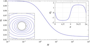
 ${\it\Omega}$
versus
 $M$
. The two insets correspond to the gas-bubble limit
 $M=\infty$
, respectively showing the streamlines
 ${\it\Psi}^{\prime }=\text{const.}$
and the variation with
 ${\it\theta}$
of the universal surface-charge density.

Substitution of (7.2) into (6.2) yields
 $$\begin{eqnarray}\left[{\it\Omega}+2\mathop{\sum }_{n=1}^{\infty }a_{n}\cos 2n{\it\theta}\right]\left[{\it\Omega}+4\left(1+\frac{1}{M}\right)\mathop{\sum }_{n=1}^{\infty }na_{n}\cos 2n{\it\theta}\right]=1-\cos 2{\it\theta}.\end{eqnarray}$$
This infinite system of nonlinear algebraic equations can be solved by comparing Fourier modes. The zeroth-mode balance gives
 $$\begin{eqnarray}{\it\Omega}^{2}+4\frac{M+1}{M}\mathop{\sum }_{m=1}^{\infty }ma_{m}^{2}=1,\end{eqnarray}$$
while for
 $n>1$
we find
 $$\begin{eqnarray}2{\it\Omega}\left(2n+\frac{M}{M+1}\right)a_{n}+4\mathop{\sum }_{m=1}^{\infty }(n+2m)a_{m}a_{n+m}+4\mathop{\sum }_{m=1}^{n-1}(n-m)a_{m}a_{n-m}=-{\it\delta}_{n,1}\frac{M}{M+1}.\end{eqnarray}$$
Because of the invariance of the universal problem to the reversal of the flow direction, it suffices to consider only the ‘positive’ branch, where
 ${\it\Omega}>0$
.
For
 $M\rightarrow 0$
(highly viscous drop) it is readily found that
 ${\it\Omega}\rightarrow 1$
while
 $a_{n}=O(M^{n})$
. In this limiting case the streamlines are concentric circles. For finite values of
 $M$
we use controlled truncation to solve the algebraic system numerically using iterations, starting from a positive
 ${\it\Omega}$
. The resulting (rather weak) dependence of angular speed
 ${\it\Omega}$
upon
 $M$
is depicted in figure 3. As
 $M\rightarrow \infty$
(inviscid gas ‘bubble’) we get
 ${\it\Omega}=0.92669$
. The two insets of figure 3 correspond to this limit. The first depicts the corresponding (non-circular) streamline pattern, and the second portrays the variation with
 ${\it\theta}$
of the universal surface-charge density
 $Q^{\prime }$
, obtained from (6.4). This limiting stationary distribution corresponding to an induced dipole (cf. figure 1) perpendicular to the applied field reflects the dynamic balance of surface-charge convection and Ohmic charging at asymptotically large
 $\mathit{Re}$
.
Given the scaling of the large-
 $\mathit{Re}$
solution and the additional rescaling employed in (6.1), it is evident that, at large
 $\mathit{Re}$
,
 $$\begin{eqnarray}{\it\omega}\sim \frac{\sqrt{S(1-RS)}}{S+1}{\it\Omega}\mathit{Re}^{-1/2},\end{eqnarray}$$
where
 ${\it\Omega}$
is rather insensitive to the value of
 $M$
, see figure 3. This allows the dependence of
 ${\it\omega}$
upon
 $\mathit{Re}$
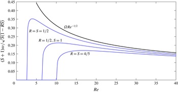
to be captured in a universal form. Thus, figure 4 presents the variation with
 $\mathit{Re}$
of the rescaled angular speed
 $(S+1){\it\omega}/\sqrt{S(1-RS)}$
using the numerical solutions of figure 2, obtained for
 $M=0.4$
and the indicated values of
 $R$
and
 $S$
. Regardless of the values of
 $R$
and
 $S$
, the rescaled speed approaches the universal asymptote
 ${\it\Omega}\mathit{Re}^{-1/2}$
(wherein
 ${\it\Omega}=0.9919$
, see figure 3), with convergence already taking place at moderately large values of
 $\mathit{Re}$
. As could be anticipated, following an earlier bifurcation to an asymmetric solution, this convergence becomes more rapid with diminishing values of
 $RS~({<}1)$
.
Collapse of the rescaled exact solutions, calculated for the indicated values of
 $R$
and
 $S$
, on the universal large-
 $\mathit{Re}$
approximation. The viscosity ratio is
 $M=0.4$
.

8. Concluding remarks
In summarizing our results, it is illustrative to go back to dimensional quantities. The present analysis for large electric Reynolds numbers is valid for field magnitudes
 $E$
that are large relative to
 $\sqrt{{\it\sigma}{\it\mu}}/{\it\epsilon}$
. At this limit, solutions exist only when charge relaxation within the suspending liquid is faster than that in the drop,
 ${\it\sigma}/{\it\epsilon}>\bar{{\it\sigma}}/\bar{{\it\epsilon}}$
. These solutions lack fore–aft symmetry and involve drop rotation, the corresponding angular velocity scaling as
 $E\sqrt{{\it\sigma}/{\it\mu}}$
. For a given set of parameters, the reverse flow is also a solution. The dependence of the scaled angular velocity upon
 $R$
and
 $S$
is obtained as a simple closed-form expression.
Numerical solutions of the exact 2D equations indeed predict a bifurcation from a fore–aft-symmetric solution to a rotating-drop solution when the electric Reynolds number is sufficiently high. Unsurprisingly, the Reynolds-number threshold for this bifurcation is lower the faster is the relaxation in the suspending liquid, namely with increasing difference between
 ${\it\sigma}/{\it\epsilon}$
and
 $\bar{{\it\sigma}}/\bar{{\it\epsilon}}$
. Regardless of the magnitude of that difference, however, the resulting value of the angular velocity eventually approaches that predicted by the asymptotic solution. We therefore predict a useful universal structure that is independent of both the conductivity and permittivity ratios.
Our interest in drop rotation has naturally directed our attention to asymmetric solutions. It is, however, worthwhile to note that, while (5.10) is incompatible with (3.1) for continuous surface distributions of the scaled fields
 $Q$
and
 $V$
, it does not exclude fore–aft-symmetric solutions involving finite (jump) discontinuities at
 ${\it\theta}=\pm {\rm\pi}/2$
. These weak solutions are reminiscent of the ‘charge shocks’ recently described by Lanauze, Walker & Khair (Reference Lanauze, Walker and Khair2015) in the 3D axisymmetric problem. Thus, with increasing
 $\mathit{Re}$
the surface-charge density approaches a fore–aft-antisymmetric distribution with a narrow transition layer about the equator. Experiments demonstrate (ibid.) that these solutions becomes unstable at large
 $\mathit{Re}$
, as manifested in the onset of drop rotation.
A desirable extension of the present work is the corresponding 3D analysis of drop rotation. Study of these issues is currently underway, with preliminary results indicating that the present scaling as
 $\mathit{Re}^{-1/2}$
is essential to the resolution of the 3D problem as well.
Acknowledgements
We are grateful to O. Schnitzer and A. M. J. Davis for their insightful suggestions. This work was supported by the Israel Science Foundation (grant no. 184/12).