



1. Introduction
Turbulent, hypersonic boundary layers form over objects, including human-made flight vehicles and meteorites, travelling through the Earth’s atmosphere at sufficiently high flight Reynolds numbers. Non-uniform surface patterns associated with boundary layer/surface instabilities have been observed on both vehicle heat shields and meteorites after Earth entry, the latter example producing regmaglypt patterns characterised by deep surface grooves (Larson & Mateer Reference Larson and Mateer1968). Observation of cross-hatching, or quasi-regularly spaced diamond-shaped surface patterns, on recovered flight vehicles spurred numerous studies of this and related phenomena via wind tunnel, rocket facility and flight tests (Canning, Tauber & Wilkins Reference Canning, Tauber and Wilkins1968; Larson & Mateer Reference Larson and Mateer1968; McDevitt Reference McDevitt1971; Nachtsheim & Larson Reference Nachtsheim and Larson1971; Williams Reference Williams1971; Stock & Ginoux Reference Stock and Ginoux1973), as well as theoretical studies (Swigart Reference Swigart1974). It is generally agreed that locally supersonic flow conditions, as well as a turbulent boundary layer, are necessary conditions for the development of cross-hatching, which has been observed on a variety of materials, including charring and non-decomposing heat shield materials, sublimating materials, and even wood (Swigart Reference Swigart1974). Cross-hatching is known to evolve into relatively deep and irregular indentations in the surface, referred to as scalloping (Larson & Mateer Reference Larson and Mateer1968; Grabow & White Reference Grabow and White1975). The scalloping mechanism is believed to be closely related to development of regmaglypts on meteorites (Larson & Mateer Reference Larson and Mateer1968).
Cross-hatching and scallop pattern length scales associated with hypersonic flight are often comparable to, or larger than, the local boundary layer thickness, distinguishing these surface patterns from rough surfaces, where the characteristic depth and length scales of the surface imperfections are typically small relative to the boundary layer thickness. For surface pattern wavelengths comparable to or greater than the boundary layer thickness, these can be considered wavy-wall flows, with accompanying pressure gradients, shock/expansion disturbances and flow curvature each producing effects across the entire boundary layer. This is in contrast to a short-wavelength rough wall, the effects of which are constrained primarily to the inner region of the boundary layer. Charru, Andreotti & Claudin (Reference Charru, Andreotti and Claudin2013) give an overview of wavy-wall boundary layers in the context of sand dune formation, including a discussion of flow regimes, assuming small-amplitude (linear response) waves where the vertical extent of the boundary layer is much greater than the penetration height of surface-induced flow disturbances. Supersonic boundary layers, however, violate this assumption due to introduction of shock/expansion waves that extend into the outer region of the boundary layer and are associated with nonlinearity in flow response even for modest wave heights.
Experimental studies of turbulent boundary layers over wavy surfaces are largely limited to low-speed flow. Wavy-walled plane channel flow, with a sinusoidal wall shape in the flow direction (referred to herein as a ‘one-dimensional (1-D) wavy wall’), was studied extensively in a series of experiments by Hanratty and co-workers (Thorsness, Morrisroe & Hanratty Reference Thorsness, Morrisroe and Hanratty1978; Frederick & Hanratty Reference Frederick and Hanratty1988). These studies focused primarily on small-amplitude surface waves and turbulence modelling approaches that capture the phase lag between surface shear stress and the surface shape. Larger-amplitude waves involving nonlinear effects (Zilker, Cook & Hanratty Reference Zilker, Cook and Hanratty1977) and flow separation on the lee side of surface waves (Buckles, Hanratty & Adrian Reference Buckles, Hanratty and Adrian1984) were also studied. Inger & Williams (Reference Inger and Williams1972) performed wind tunnel experiments on transonic turbulent boundary layers up to Mach 1.8 over a small-amplitude sinusoidal surface, measuring surface pressure and wall temperature perturbations. They showed that a linear mathematical model was successful in describing the phase of surface pressure distributions, but overpredicted the pressure amplitude due to nonlinear effects in the transonic regime that appear even for wave amplitudes of only 3 % of the surface wavelength. We were unable to find any computational or experimental studies of fully turbulent boundary layers over 1-D wavy wall surfaces in supersonic or hypersonic regimes.
Incompressible wavy-walled channel direct numerical simulations (DNS) studies have been performed, and illustrate differences in turbulence structure and organisation of turbulent motion between flat and wavy-walled flow. De Angelis, Lombardi & Banerjee (Reference De Angelis, Lombardi and Banerjee1997) considered geometries with ratio of surface wavelength to channel half-height (
 $\lambda /h$
) 0.5 and 1.0, and observed a redistribution of streamwise to spanwise velocity fluctuation energy, and the appearance of streamwise vortical structures generated over the front faces of the surface, which they attributed to pressure strain and boundary layer reattachment dynamics, respectively. Cherukat et al. (Reference Cherukat, Na, Hanratty and McLaughlin1998), in a DNS study of a similar wavy-walled channel (
 $\lambda /h = 1$
), noted the presence of ‘velocity bursts’ associated with the separation shear layer in the wave troughs, with influence extending far from the wall. More recently, Zhang et al. (Reference Zhang, Wu, Liu and Wang2022) performed LES of a number of wavy-walled channels with large enough wave amplitude to induce separation. They observed streamwise vortices that originated from separation and reattachment points, and provided evidence that the vortices are triggered by the Görtler centrifugal instability mechanism, which generates streamwise vorticity in a boundary layer experiencing concave streamline curvature (Saric Reference Saric1994).
Compressible channel flow with sinusoidal walls has been simulated by several authors. Tyson & Sandham (Reference Tyson and Sandham2013) performed DNS of channel flow with wavy top and bottom walls at bulk Mach numbers 0.3, 1.5 and 3.0,
 $\lambda /h = 1, 2, 4$
, and
 $a/h=0.04,0.08$
, where
 $a$
is the sinusoidal surface wave amplitude, and
 $h$
is the channel half-height. A prominent feature of the simulated flow fields for the supersonic cases was the presence of strong oblique shocks emanating from the opposite wall, causing appreciable perturbation to the Reynolds stress fields. Sun et al. (Reference Sun, Zhu, Hu and Zhang2018) performed a compressible DNS study counterpart to the Cherukat et al. (Reference Cherukat, Na, Hanratty and McLaughlin1998) configuration, generating solutions up to bulk Mach number 1.5. Their results for supersonic cases indicate significant contributions to turbulence kinetic energy production from terms other than the usual shear production due to interaction of the turbulence with the shock and expansion waves induced by the surface; however, these contributions tended to cancel when averaged over a wavelength. Aghaei-Jouybari et al. (Reference Aghaei-Jouybari, Yuan, Li, Brereton and Jaberi2023) also performed DNS of a supersonic wavy-walled channel at bulk Mach number 1.5,
 $a/h=0.05$
, and for
 $\lambda /h = 1,2$
. They demonstrated the generation of a strong and quasi-stationary shock pattern throughout the channel, which has a significant influence on the temperature field, and postulated that the presence of the shock waves invalidates the wall similarity hypothesis, which posits that the effects of surface non-uniformities are evident only in the inner layer.
In this paper, we present LES of a hypersonic turbulent boundary layer over a wavy surface for six combinations of surface wavelength and amplitudes. The primary aim of the study is to close gaps in knowledge related to surface quantity distributions of engineering interest (wall shear stress, heat flux and pressure fluctuations), and their relationship to the altered turbulence structure induced by the wavy-wall shape and associated shock/expansion disturbances. The present computational investigation is unique in several ways. The configuration is a boundary layer flow, which is closer to the external aerodynamic configurations of interest, and avoids potential contamination by opposite wall effects in a channel flow, which can be significant for supersonic flows. We consider a cold-wall flow, allowing for investigation of wall heat flux in conditions typical of high Mach number flight. Finally, the 1-D sinusoidal geometry allows for evaluation of flow characteristics relative to existing studies for low-Mach-number flow, and extends previous results to the hypersonic regime.
Section 2 presents the simulation method, as well as the geometries and flow conditions for the six cases simulated. Subsection 3.1 presents the overall flow structure, while § 3.2 provides an assessment of solution quality. In § 3.3, the behaviour of mean wall quantities is explored, including documentation of the phases of wall quantities relative to the wall shape. Subsection 3.4 presents mean velocity and stress fields, shedding light on the perturbations of these fields due to the wavy wall and associated shock/expansion disturbances. Subsection 3.5 presents elements of the turbulence kinetic energy budget that are modulated by the wavy wall, while § 3.6 explores the wall pressure fluctuation statistics and associated phenomenology. The presence and role of streamwise-oriented vortical structures over the wavy surfaces, and their relationship to streamline curvature, are discussed in § 3.7. Conclusions follow in § 4.
2. Methodology
2.1. Numerical model
The compressible Navier–Stokes equations for a perfect, heat-conducting gas are
 \begin{equation} \frac {\partial \rho }{\partial t} + \frac {\partial (\rho u_i)}{\partial x_i} =0, \end{equation}
 \begin{equation} \frac {\partial (\rho u_i)}{\partial t} + \frac {\partial (\rho u_i u_{\!j})}{\partial x_{\!j}} = -\frac {\partial P}{\partial x_i} + \frac {\partial \sigma _{ij}}{\partial x_{\!j}}, \end{equation}
 \begin{equation} \frac {\partial (\rho E)}{\partial t} + \frac {\partial (\rho E u_{\!j} +Pu_{\!j})}{\partial x_{\!j}} = \frac {\partial (\sigma _{ij}u_i -q_{\!j})}{\partial x_{\!j}}, \end{equation}
where Einstein summation is implied. The spatial coordinates
 $(x_1, x_2, x_3)=(x,y,z)$
denote the streamwise, transverse and spanwise directions, respectively,
 $u_i$
are the velocity components, and
 $\rho$
,
 $P$
and
 $T$
denote the fluid density, pressure and temperature. The total energy per unit mass is given by
 $E=C_vT + u_iu_i/2$
, where
 $C_v$
is the specific heat at constant volume, and the viscous stress tensor and heat flux vector are given by
 \begin{equation} \sigma _{ij}=\mu \left (\frac {\partial u_i}{\partial x_{\!j}}+\frac {\partial u_{\!j}}{\partial x_i}-\frac {2}{3}\frac {\partial u_k}{\partial x_k}\delta _{ij}\right )\!, \end{equation}
 \begin{equation} q_{\!j}=-\kappa _T\frac {\partial T}{\partial x_{\!j}}, \end{equation}
where
 $\delta _{ij}$
is the Kronecker delta,
 $\kappa _T=C_{\!p}\mu /\textit{Pr}$
is the thermal conductivity,
 $\mu$
is the molecular viscosity,
 $\textit{Pr}=0.72$
is the Prandtl number, and
 $C_{\!p}$
is the specific heat at constant pressure. The molecular viscosity is computed from Sutherland’s law
 \begin{equation} \mu =C_1\frac {T^{3/2}}{T+S}, \end{equation}
where
 $C_1=1.458\times 10^{-6}\ \rm kg\ m^{-1}\ s^{-1}\ {K}^{-1/2}$
, and
 $S=110.4\,\rm K$
.
We solve these equations using a cell-centred finite-volume form implemented in the Sandia Parallel Aerodynamics and Reentry Code (Freno, Carnes & Weirs Reference Freno, Carnes and Weirs2021). In our approach, inviscid terms are discretised with a hybrid low-dissipation-shock-capturing scheme. In smooth regions of the flow, we employ the low-dissipation fourth-order method of Subbareddy & Candler (Reference Subbareddy and Candler2009), while near shock wave discontinuities, the second-order flux-vector splitting scheme of Steger & Warming (Reference Steger and Warming1981) is activated via a modified form of the Larsson dissipation switch (Larsson, Vicquelin & Bermejo-Moreno Reference Larsson, Vicquelin and Bermejo-Moreno2011). Viscous fluxes are discretised with a second-order approach, and time integration is performed with the classical fourth-order Runge–Kutta method. In place of a subgrid-scale model, we rely on the numerical dissipation provided by the shock-capturing scheme to remove energy at unresolved scales; the blending between the flux schemes is constrained so that the dissipative flux provides a minimum of 1 % contribution to the total inviscid flux.
We employ structured, curvilinear, body-fitted grids in this work, and periodic boundary conditions are imposed in the spanwise direction. While streamwise and spanwise grid lines are conformal with the wavy geometry at the wall, and gradually conform to the geometry of the upper surface of the domain, transverse grid lines do not guarantee orthogonality at the wall; however, the grid resolution is sufficient to mitigate cell skew.
To mimic the spatial evolution of cross-hatch pattern amplitudes observed in low-temperature ablators (Stock Reference Stock1975), we gradually introduce the wavy wall over five wavelengths using a hyperbolic tangent function (see figure 1), which also serves to mitigate large slope changes upon wavy-wall inception. To promote solution stability near the outflow plane, the wavy-wall amplitude is gradually degraded over five wavelengths with a hyperbolic tangent function.
Instantaneous temperature field for the L1K08 case. The flow is from lower left to upper right, and the wall is coloured grey.

Figure 1 Long description
A heat map illustrating the instantaneous temperature field for the L1K08 case. The flow direction is from the lower left to the upper right. The wall is colored grey. The temperature scale ranges from 60 Kelvin to 200 Kelvin, with blue indicating lower temperatures and red indicating higher temperatures. The heat map shows variations in temperature across the flow, with distinct regions of different temperature intensities. The x, y, and z axes are labeled to provide spatial context. The temperature distribution reveals areas of higher and lower temperature gradients, indicating the interaction between the flow and the wavy surface.
The total wavy region comprises 15 wavelengths (
 $L_x=15\lambda$
), where the middle five wavelengths are expressed at full amplitude. As documented in Appendix B, the statistical structure of the boundary layer and underlying wall quantities reaches a quasi-periodic state by the last full-amplitude wave element (see figure 2). This does not necessarily imply that an equilibrium state has been reached due to the continuous strain fields imposed by the alternating expansion and compression regions on the scale of the boundary layer thickness or greater. Thus the present simulation set-up does not represent an equilibrium turbulent flow, as in classical rough-wall flows, or a strictly periodic flow, as in channel flow studies. Rather, the flow is a spatially developing turbulent boundary layer under periodic forcing from the underlying surface, which reaches a quasi-periodic state by the final full-amplitude element. We focus the analysis in the following sections on the properties of the flow over this last representative wave element.
Schematic of the numerical domain. The wall is coloured black. The vertical magenta line denotes the inflow plane, the vertical red line denotes the upstream flow state, the vertical black line denotes the wavy-wall inception, and the vertical blue lines bound the final full-amplitude wavy-wall element.

Figure 2 Long description
The schematic illustrates a numerical domain with various labeled sections. The wall is colored black. The vertical magenta line represents the inflow plane, the vertical red line denotes the upstream flow state, the vertical black line indicates the wavy-wall inception, and the vertical blue lines mark the boundaries of the final full-amplitude wavy-wall element.
The vertical and spanwise extents of the numerical domains are chosen as
 $L_y=10\delta _1$
and
 $L_z=5\delta _1$
, where
 $\delta _1=3.83\,\rm mm$
denotes the incoming boundary layer thickness to the wavy wall, whereas the boundary layer thickness at the inflow plane is
 $\delta _0=1.25\,\rm mm$
. Additionally, at the inflow plane, the boundary layer displacement thickness and momentum thickness are
 $\delta ^*_0=0.65\,\rm mm$
and
 $\theta ^*_0=0.068\,\rm mm$
, respectively.
Turbulent fluctuations are prescribed on the inflow plane using the synthetic digital filtering method (SDFM) of Adler et al. (Reference Adler, Gonzalez, Stack and Gaitonde2018), where turbulent statistics required for SDFM initialisation are derived from a precursor Reynolds-averaged Navier–Stokes (RANS) simulation. To ensure a sufficient relaxation length for the incoming turbulent boundary layer, the inflow plane is located
 $78\delta _0$
upstream of the wavy-wall initiation, corresponding to approximately
 $36\delta _1$
.
Finally, we note that throughout this paper, due to the presence of shocks and expansions throughout the boundary layer, we calculate the boundary layer thickness (
 $\delta$
) using a total enthalpy threshold, where the boundary layer edge is defined as the transverse location where the total enthalpy of the local flow reaches 99.5 % of the freestream value. Compared to defining the boundary layer edge using the classical
 $0.99u_\infty$
threshold (
 $\delta _{99}$
), we find that
 $\delta _0/\delta _{0,99}=1.02$
and
 $\delta _1/\delta _{1,99}=1.01$
, demonstrating minimal sensitivity to the boundary layer edge detection method. The flow properties at the boundary layer edge are subsequently utilised for computation of the displacement and momentum thickness.
2.2. Flow conditions and wavy-wall topology
The flow conditions were chosen to closely match the Mach 5.84 turbulent boundary layer from the DNS study of Zhang, Duan & Choudhari (Reference Zhang, Duan and Choudhari2018). A detailed description of the incoming turbulent boundary layer properties is provided in table 1. These flow conditions correspond to the ‘upstream’ flow state, and are located
 $2.6\delta _1$
upstream of the wavy-wall inception (see figure 2). We maintain upstream friction Reynolds number
 $\textit{Re}_\tau =450$
for all cases, and vary the peak-to-trough wall amplitude (
 $k$
) and wall wavelength (
 $\lambda$
). The 1-D wavy-wall topology is defined by
 \begin{equation} y=0.5k \sin \left (\frac {2\pi x}{\lambda }\right )\!. \end{equation}
Details of the wavy-wall topologies are provided in table 2. The effective slope (
 $\textit{ES}$
) of the wavy surface is given by
 $\textit{ES}=( {1}/{\lambda })\int _{0}^{\lambda } (| {\partial y}/{\partial x}|)\, {\rm d}x$
. The geometric parameters of the wavy-wall topology were chosen to lie within the ranges of streamwise length scale and wave amplitude experimentally observed in cross-hatching patterns on ablating surfaces (Grabow & White Reference Grabow and White1973; White & Grabow Reference White and Grabow1973). Specific choices of amplitude and wavelength were also made to facilitate comparisons to the supersonic 1-D wavy-wall channel DNS of Tyson & Sandham (Reference Tyson and Sandham2013).
Incoming boundary layer quantities to the wavy wall. This location is denoted the ‘upstream’ location throughout this work, and resides
 $2.6\delta _1$
upstream of the wavy-wall inception (see figure 2). The variables
 $\delta ^*_1$
and
 $\theta ^*_1$
denote the displacement and momentum thickness, respectively.

Table 1 Long description
The table presents incoming boundary layer quantities for a wavy wall, detailing parameters such as Mach number, Reynolds number, density, velocity, temperature, and various boundary layer thicknesses. It includes eight columns: Mach number, Reynolds number, free stream density, free stream velocity, free stream temperature, boundary layer thickness, displacement thickness, momentum thickness, and friction velocity. The table has one row of data, providing specific values for each parameter. The data is used to describe the upstream flow state located 2.6 times the boundary layer thickness upstream of the wavy-wall inception.
The 1-D wavy-wall topology parameters.

Table 2 Long description
The table presents flow conditions for six different cases, comparing parameters such as k/delta1, delta1/lambda, lambda/delta1, lambda/k, ES, and k+. The table has six rows and seven columns. The columns are labeled as Case, k/delta1, delta1/lambda, lambda/delta1, lambda/k, ES, and k+. Each row corresponds to a specific case with varying values for these parameters. The cases are labeled as LIK04, LIK08, LIK16, L2K04, L2K08, and L2K16. The values for k/delta1 range from 0.04 to 0.16, delta1/lambda values are either 0.9 or 0.45, lambda/delta1 values are either 1.11 or 2.22, lambda/k values range from 27.7 to 55.5, ES values range from 0.036 to 0.290, and k+ values range from 20 to 80. The table provides a detailed comparison of the geometric parameters of the wavy-wall topology used in the study.
For comparative analysis, an additional flat plate simulation is conducted to gather flow statistics at equivalent wavy-wall streamwise locations.
2.3. Averaging approach
When analysing the turbulent flow over a non-uniform wall shape, it is useful to decompose the spatio-temporal flow quantities in ways that isolate macroscopic effects of wall non-uniformities on the turbulence dynamics. In this work, we employ the classical Favre
 $(\tilde {{\cdot }})$
and Reynolds
 $(\bar {{\cdot }})$
operators to decompose an instantaneous flow quantity over a spanwise homogeneous element into
 \begin{equation} q(x,y,z,t)=\tilde {q}(x,y)+q^{\prime\prime}(x,y,z,t), \quad q(x,y,z,t)=\bar {q}(x,y)+q^\prime(x,y,z,t), \end{equation}
where averaging is performed in time and in the homogeneous direction. The averaged quantities can be further decomposed into a wave-averaged mean component, and a residual dispersive component defined by
 \begin{equation} \tilde {q}(x,y) = \langle \tilde {q} \rangle (\hat {y}) + \tilde {q}^d(x,y), \quad \bar {q}(x,y) = \langle \bar {q} \rangle (\hat {y}) + \bar {q}^d(x,y), \end{equation}
where
 $\langle {\cdot }\rangle$
denotes a wave average at a relative height from the wavy wall for a given streamwise location, with the relative height given by
 $\hat {y} = y - y_{wall}$
, similar to the curvilinear coordinate spatial averaging procedure of Ma et al. (Reference Ma, Xu, Sung and Huang2023). We choose this approach over averaging at a fixed, absolute
 $y$
-coordinate to allow for a consistent and well-defined spatial averaging operation over a wave element. This approach is demonstrated in figure 3, which shows how the averaging operator casts the flow into components retaining the features of a classical flat plate turbulent boundary layer (figure 3
b), and a dispersive component (figures 3
c,d), which represents mean flow spatial variation as a result of surface non-uniformities.
Demonstration of the spatio-temporal averaging procedure for the L1K16 case: (a) Favre-averaged streamwise velocity, (b) wave-averaged streamwise velocity, (c) dispersive streamwise velocity, and (d) dispersive transverse velocity. The wavy wall is outlined in black.

Figure 3 Long description
The image contains four heat maps, each representing different velocity components over a wavy wall. The first heat map shows the Favre-averaged streamwise velocity, the second shows the wave-averaged streamwise velocity, the third depicts the dispersive streamwise velocity, and the fourth illustrates the dispersive transverse velocity. The wavy wall is outlined in black. Each heat map uses a color gradient to represent velocity magnitudes, with the x-axis labeled as x/λ and the y-axis labeled as y/δ. The color bars on the right of each heat map indicate the velocity ratios, with red representing higher velocities and blue representing lower velocities. The heat maps provide a visual demonstration of the spatio-temporal averaging procedure for the L1K16 case.
This triple decomposition can be further leveraged to split the total stress tensor into respective Reynolds (turbulent) and dispersive components (Türk et al. Reference Türk, Daschiel, Stroh, Hasegawa and Frohnapfel2014; Chan & Chin Reference Chan and Chin2023):
 \begin{equation} \tau _{ij}=\langle \bar {\rho }\rangle \langle \widetilde {u''_iu''_{\!j}}\rangle +\langle \bar {\rho }\rangle \langle \widetilde {u^d_i}\,\widetilde {u^d_{\!j}}\rangle, \end{equation}
which will be utilised in the following sections to assess grid convergence and compare total stress modulation due to wavy-wall topology.
3. Results
3.1. Flow structure
The time-averaged dilatation is shown in figure 4 to depict the overall flow structure. The interaction of the incoming boundary layer with the wavy wall generates a series of alternating shock and expansion waves, with shocks forming during flow recompression above the trough, and expansions forming over the wall crest. Given that the sonic line of the incoming boundary layer resides at
 $y^+=10$
, and that
 $k^+ \geqslant 20$
for all cases, the formation of these waves is expected. A dual shock structure is observed for the L2K16 case due to flow separation in the trough. For all wall amplitudes, the shock waves protrude through the entire boundary layer, thereby perturbing the turbulent motions. Similar perturbations of a turbulent boundary layer over diamond-patterned roughness were observed at Mach 4.9 conditions by Peltier, Humble & Bowersox (Reference Peltier, Humble and Bowersox2016).
Time-averaged dilatation for the (a) L2K04, (b) L2K08 and (c) L2K16 cases. The wavy walls are initiated at
 $x/\delta _1\approx 36$
.

Figure 4 Long description
The image consists of three heat maps labeled (a), (b), and (c), each representing time-averaged dilatation for the cases L2K04, L2K08, and L2K16 respectively. The x-axis is labeled x/delta1 and ranges from 40 to 60, while the y-axis is labeled y/delta1 and ranges from 0 to 2. Each heat map displays a gradient of values from -500 to 500, with darker shades indicating lower values and lighter shades indicating higher values. The wavy walls are initiated at x/delta1 approximately 36. The heat maps show distinct patterns of dilatation, with variations in intensity and distribution across the three cases. The overall trend in each heat map reveals a series of diagonal bands that shift and change in intensity, reflecting the complex interactions within the turbulent, hypersonic boundary layers.
3.2. Solution verification and grid convergence
Solution verification studies are conducted to assess grid sensitivity in the LES solutions. Four different levels of grid resolution are examined (see table 3). Increasing levels of grid refinement are considered, spanning nominal wall-resolved LES resolution based on best practices (Choi & Moin Reference Choi and Moin2012), to DNS-like resolution. For the R1, R2 and R3 grids, streamwise and spanwise grid spacings are constant throughout the domain. For the R2p5 grid, while the spanwise grid spacing remains constant throughout the domain, the streamwise spacing transitions from R2 spacing upstream of the wavy wall, to R3 spacing over the wavy wall. The purpose for this transition, which occurs approximately
 $2\delta _1$
upstream of the wavy wall, is to reduce the computational cost of simulating the incoming boundary layer, while retaining DNS-like resolution over the wavy wall.
Grid density metrics computed using the upstream viscous length scale. The subscripts
 $u$
and
 $wv$
denote upstream and wave-averaged values, respectively.

Table 3 Long description
The table presents grid density metrics for four different levels of grid resolution labeled R1, R2, R2p5, and R3. The metrics include Δx+_u, Δx+_wv, Δy+, Δz+_u, Δz+_wv, Nx, Ny, and Nz. R1 has values 19.3, 14.9, 0.1–10, 11.5, 9.0, 1355, 251, and 223 respectively. R2 shows values 11.5, 7.6, 0.1–10, 9.2, 6.2, 2257, 251, and 334. R2p5 has values 6.3, 4.8, 0.1–10, 3.9, 3.2, 3049, 251, and 667. R3 presents values 6.3, 4.7, 0.1–10, 4.7, 3.1, 4515, 251, and 667. The table highlights the variations in grid spacing and resolution across different grids.
To validate the accuracy of the incoming turbulent boundary layer across grid densities, we compare LES results to the DNS results of Zhang et al. (Reference Zhang, Duan and Choudhari2018) using a mean velocity transformation that is suitable for compressible flows. Although numerous compressible velocity transformations have been developed, including the classical transformation of Van Driest (Reference Van Driest1951), we choose the approach of Hasan et al. (Reference Hasan, Larsson, Pirozzoli and Pecnik2023), denoted ‘HLPP’, due to its success in collapsing the mean velocity field of high-speed diabatic boundary layers to their incompressible counterparts. The HLPP transformation is given by
 \begin{equation} \bar {U}^+_{\textit{HLPP}} = \int _{0}^{\bar {u}^+} \left (\frac {1+\kappa y^* D(y^*,M_\tau )}{1+\kappa y^* D(y^*,0)}\right )\left (1-\frac {y}{\delta ^*_\nu }\frac {{\rm d}\delta ^*_\nu }{{\rm d}y} \right ) \sqrt {\frac {\bar {\rho }}{\rho _w}}\, {\rm d}\bar {u}^+, \end{equation}
where the von Kármán constant is
 $\kappa =0.41$
, the semi-local length scale of Trettel & Larsson (Reference Trettel and Larsson2016) is
 $\delta _\nu ^*=\overline {\mu }/(\overline {\rho }u_\tau ^*)$
, the semi-local friction velocity is
 $u_\tau ^*=\sqrt {\tau _w/\overline {\rho }}$
, the semi-local wall coordinate is
 $y^*=y/\delta _\nu ^*$
, the eddy-viscosity damping function is
 $D(y^*,M_\tau )= [1-\exp ( {-y^*}/({A^++f(M_\tau )} )) ]^2$
, the friction Mach number is
 $M_\tau =u_\tau /\sqrt {\gamma R T_w}$
,
 $f(M_\tau )=19.3M_\tau$
, and
 $A^+=17$
.
Figure 5(a) shows the HLPP-transformed mean velocity profiles of the upstream boundary layer at
 $\textit{Re}_\tau =450$
. The transformed profiles reproduce the expected mean velocity profile, including linear behaviour in the viscous sublayer, and logarithmic behaviour for
 $y^*=30{-}150$
. The viscous-scaled root mean squares (r.m.s) of the Favre-averaged velocity fluctuations are shown in figures 5(b–d). While slight sensitivity to grid density is evident by the overprediction of peak
 $u^+_{\textit{rms}}$
and
 $w^+_{\textit{rms}}$
, differences are within 3 % on the R3 grid, and our results closely replicate the DNS results of Zhang et al. (Reference Zhang, Duan and Choudhari2018). Additional verification results for the LES solution over the wavy wall are deferred to Appendix A. Our primary conclusion is that results on the R2p5 grid closely replicate those on the R3 grid, thus we employ the R2p5 grid resolution throughout the remainder of this study.
Comparison of the upstream boundary layer statistics to the DNS results of Zhang et al. (Reference Zhang, Duan and Choudhari2018) as a function of the semi-local wall coordinate. (a) The HLPP-transformed mean streamwise velocity profile. The dashed magenta line denotes the viscous sublayer region (
 $u^+=y^+$
), and the dotted magenta line denotes the logarithmic region (
 $u^+=({1}/{\kappa })\ln(y^+)+5.1$
). Plots of (b)
 $u^+_{\textit{rms}}$
, (c)
 $v^+_{\textit{rms}}$
, (d)
 $w^+_{\textit{rms}}$
. Refer to table 3 for a description of grid densities.

Figure 5 Long description
The image contains four line graphs comparing boundary layer statistics to the DNS results of Zhang et al. (2018) as a function of the semi-local wall coordinate. Graph (a) shows the HLPP-transformed mean streamwise velocity profile with a dashed magenta line denoting the viscous sublayer region and a dotted magenta line denoting the logarithmic region. Graphs (b), (c), and (d) plot the root mean square values of the streamwise, wall-normal, and spanwise velocity fluctuations, respectively. The x-axis represents the semi-local wall coordinate, and the y-axis represents the respective velocity fluctuations. The data series are color-coded with red, blue, cyan, black, and green lines representing different datasets or conditions. The graphs illustrate how the velocity fluctuations vary across different regions of the boundary layer. All values are approximated.
3.3. Mean wall quantities
The mean wall pressure, wall shear stress, and wall heat flux are of primary importance in determining aerodynamic and heating loads on a non-uniform flight vehicle surface, and are examined first. Figure 6 shows time- and spanwise-averaged wall quantities over the final full-amplitude wavy element normalised by their respective local flat plate values, denoted by the subscript ‘fp’. Unless otherwise noted, all assessments of the flow over the wavy wall are examined over the final full-amplitude wavy element (see figure 2). Additionally, when examining local flow quantities over a wave,
 $x/\lambda =0$
denotes the upstream wave crest, while
 $x/\lambda =1$
denotes the downstream wave crest. The series of shock waves and expansion fans has a clear effect on the local wall pressure (figures 6
a,b), with flow expansion creating a favourable pressure gradient (FPG) over the wave crest, and flow compression creating an adverse pressure gradient (APG) in the trough. These pressure gradients influence the streamwise wall shear stress (figures 6
c,d), which reaches maximum value under the FPG near the crest, and minimum values in the trough, with flow separation occurring for the highest
 $\textit{ES}$
cases (i.e. L1K08, L1K16 and L2K16). Mean wall pressure profiles for attached and separated flows behave differently. For attached flows (L1K04, L2K04, L2K08), the wall pressure profiles have a sinusoidal-like shape, along with a consistent maximum pressure location (
 $x/\lambda \approx 0.8$
), and a slight sensitivity of the minimum pressure location (
 $x/\lambda \approx 0.3$
). However in separated flows, the profile shapes and the locations of wall pressure minima diverge from their attached counterparts. This is most evident in the L1K16 case, where the zero-pressure-gradient region in the trough is indicative of separated flow. Several trends are discerned as a function of wall topology. For a fixed wavelength, as the wall height is increased, the maximum wall pressure monotonically increases from its flat wall value. For a fixed wall amplitude, increasing the wavelength has different impacts on the wall pressure due to the flow behaviour in the trough. When the flow is attached, increasing the wavelength reduces the pressure extrema values, whereas when the flow is separated, increasing the wavelength increases the pressure extrema values.
Wall stress metrics for the different cases. The subscripts
 $f$
and
 $p$
denote wall stress contributions from friction and pressure components, respectively, with
 $D_t=D_{\!f}+D_{\!p}$
. The wall shear stress over the equivalent flat plate region is given by
 $D_{\!fp}$
.

Table 4 Long description
The table presents wall stress metrics for various cases, with columns labeled L1K04, L1K08, L1K16, L2K04, L2K08, and L2K16. It includes three rows of data: the first row shows the ratio of wall stress from friction to total wall stress (Df/Dt), the second row shows the ratio of wall stress from pressure to total wall stress (Dp/Dt), and the third row shows the ratio of total wall stress to wall shear stress over the equivalent flat plate region (Dt/Dfp). Notable trends include higher friction contributions in L2K04 and lower pressure contributions in L2K04.
Time- and spanwise-averaged (a,b)
 $P_w$
and (c,d)
 $\tau _{w,x}$
, normalised by flat plate values, for the (a,c) shorter wavelength L1 and (b,d) longer wavelength L2 cases. The magenta line depicts the normalised local wall height (
 $y/k$
).

Figure 6 Long description
The image contains four line graphs that illustrate experimental studies of turbulent boundary layers over wavy surfaces. The graphs show time- and spanwise-averaged values of Pw and τw,x, normalized by flat plate values, for two cases: shorter wavelength (L1) and longer wavelength (L2). The x-axis represents the normalized distance x/λ, while the y-axis on the left represents the normalized values of Pw/Pw,fp and τw,x/τw,x,fp. The y-axis on the right represents the normalized local wall height y/k, depicted by a magenta line. Each graph compares different cases: (a) and (c) for the shorter wavelength L1, and (b) and (d) for the longer wavelength L2. The blue, red, and black lines represent different experimental conditions. The magenta line shows the normalized local wall height, indicating the surface shape. The graphs highlight the phase lag between surface shear stress and the surface shape, as well as nonlinear effects and flow separation on the lee side of surface waves. All values are approximated.
The modulation of wall shear stress and wall pressure over the wavy wall impacts the total wall stress (
 $D_t$
), comprising friction (
 $D_{\!f}$
) and pressure (
 $D_{\!p}$
) contributions, given by
 \begin{equation} D_t=D_{\!f}+D_{\!p}=\frac {1}{A_s}\int _S \overline {\tau _{w,x}} \,{\rm d}S -\frac {1}{A_s}\int _S \overline {P_w} n_x\,{\rm d}S, \end{equation}
where
 $A_s$
is the wetted area of a wave element, and
 $n_x$
is the streamwise component of the local wall-normal unit vector. Table 4 reports the wall stress contributions of the different wavy-wall topologies. For a fixed wavelength, as the wall amplitude increases, the relative pressure contribution increases, while the relative friction contribution decreases. In fact, for cases with
 $\textit{ES}\geqslant 0.145$
(see table 2), we observe that the pressure contribution exceeds the friction contribution. For a fixed wall amplitude, we observe that larger wavelengths reduce the pressure contribution. The ratio of the total wall stress over the wavy wall to that of a flat plate (
 $D_t/D_{\!fp}$
) shows that with the exception of the L1K16 case, the total wall stress increases with increasing wall amplitude. The deviation of L1K16 from this trend results from the large region of separated flow contributing a non-negligible negative contribution to
 $D_{\!f}$
.
Figure 7 compares the ratio
 $D_{\!p}/D_t$
with selected results from the 1-D wavy-wall channel study of Tyson & Sandham (Reference Tyson and Sandham2013). The wave height and length are normalised by either the channel half-height
 $h$
, or, for the present results, the upstream boundary layer thickness
 $\delta _1$
. The presented wavy-channel results are for bulk Mach number 3.0. All simulation results show the expected trend of increasing relative pressure contribution with wave height. The short-wavelength boundary layer cases at the larger wave height (
 $k=0.16\delta _1$
) show a nonlinear dependence of the pressure contribution and indications of an asymptotic behaviour for large wave height. The boundary layer results, like the channel results, show a larger pressure contribution for short wavelength due to the larger effective slope, although the channel results show consistently higher pressure contribution than the boundary layer for a similar wave geometry. This difference can be attributed to the difference in Mach number between the two studies, as well as the different flow configurations. In our spatially developing boundary layer, the waves emanating from the wavy wall propagate without reflection into the outer inviscid flow, whereas in the channel flow of Tyson & Sandham (Reference Tyson and Sandham2013), the waves emanating from the wall propagate to the opposite wall, resulting in a series of reflected shocks across the channel, and a modulation of the wall pressure distribution.
Ratio of the pressure wall stress (
 $D_{\!p}$
) to the total wall stress (
 $D_t$
) over 1-D wavy walls. The circles are the present results, while the squares are the results of Tyson & Sandham (Reference Tyson and Sandham2013) for a channel flow with half-height
 $h$
and bulk Mach number 3.0.

Figure 7 Long description
A line graph showing the ratio of pressure wall stress to total wall stress over one-dimensional wavy walls. The x-axis represents the dimensionless wavenumber, while the y-axis represents the ratio of pressure wall stress to total wall stress. The graph includes two data series: one represented by black circles and squares, and another by red circles and squares. The black circles and squares represent the present results, while the red circles and squares represent the results of Tyson & Sandham (2013) for a channel flow with half-height h and bulk Mach number 3.0. The black circles and red circles show data for different wavelength-to-thickness ratios, while the black squares and red squares show data for another set of wavelength-to-thickness ratios. All values are approximated.
The degree of nonlinearity in the response of the mean pressure to the wavy surface is assessed by comparing the LES solutions to linear inviscid perturbation theory. For small perturbations to a flat plate with nominal location
 $y=0$
of the form
 $y = \epsilon \cos (\alpha x )$
, the pressure coefficient for inviscid grazing flow is given by (Liepmann & Roshko Reference Liepmann and Roshko1957)
 \begin{equation} C_{\!p} = \frac {-2\epsilon \alpha }{\sqrt {M_\infty ^2-1}} \sin \left (\alpha x\right )\!. \end{equation}
Figure 8 shows the pressure coefficient distributions over a wave for the smallest
 $\textit{ES}$
cases (L1K04, L2K04 and L2K08), comparing the linear theory, a solution to the full Euler equations, and the present LES results. There are significant differences between the linear solution and the Euler equation solution for case L1K04, indicating the presence of nonlinear inviscid effects for this case and other cases with similar or larger
 $\textit{ES}$
(L1K08, L1K16, L2K08, L2K16). Case L2K04, on the other hand, shows very close agreement in phase between the linear and Euler equation solutions, with modest differences in the peak pressure, indicating a mostly linear inviscid response of the flow for this case. The LES pressure distributions have peaks slightly downstream of the peak at maximum surface slope for the linear inviscid solution, and peak pressure coefficients that are substantially less than the peaks for the linear solution due to the reduction in dynamic pressure within the viscous boundary layer. The present LES result for case L2K04 extends the experimental results of Inger & Williams (Reference Inger and Williams1972) for wall pressure phase to higher Mach number, with the caveat that the currently considered isothermal cold-wall boundary condition differs from the nominally adiabatic conditions of that study.
Pressure coefficient (
 $C_{\!p}$
) obtained from LES results (blue), linear inviscid theory (black), and the Euler equations (red) for (a) L2K04, (b) L1K04 (solid) and L2K08 (dashed).

Figure 8 Long description
The image contains two line graphs labeled (a) and (b). Each graph plots the pressure coefficient (Cp) against the normalized distance (x/λ). In graph (a), three lines represent data from LES results (blue), linear inviscid theory (black), and the Euler equations (red) for case L2K04. In graph (b), two lines represent data from L1K04 (solid blue) and L2K08 (dashed blue). The graphs show how the pressure coefficient varies along the normalized distance for different methods and cases. The lines indicate the differences in pressure coefficient values obtained from these methods, highlighting variations and trends in the data.
The phases of the mean wall quantities relative to the wave shape profile play an important role in the thermal/material response of an underlying ablating surface. To more clearly elucidate phase differences between the quantities, we plot normalised perturbations of wall quantities about mean values, defined by
 \begin{equation} \phi^\prime(x)=\frac {\phi (x)-\langle \phi (x)\rangle }{\max(\phi (x))}, \end{equation}
where
 $\phi (x)$
is a generic wall quantity. Figures 9(a–c) show the perturbed surface pressure, shear stress magnitude and heat flux distributions for the L1 family of cases. In each case, the peak wall pressure on the windward face of the wave precedes the peak wall heat flux and wall shear stress locations, which lie closer to the surface peak. The peak wall heat flux occurs upstream of the peak wall shear stress, with relative phase angles between these two quantities of
 $35.8^\circ, 29.7^\circ, 19.3^\circ$
for cases L1K04, L1K08, L1K16, respectively. The behaviour of the heat flux peak leading the shear stress peak has also been observed in incompressible wavy-channel measurements (Thorness & Hanratty Reference Thorsness and Hanratty1979) and DNS (Chedevergne et al. Reference Chedevergne, Stuck, Olazabal-Loumé and Couzi2023), but to our knowledge, the underlying physical mechanisms have not been explained. Corresponding plots for the longer-wavelength L2 family of cases are shown in figures 9(d–f). Qualitatively, the wall quantity phase behaviour is similar to the L1 cases. Peak wall quantity perturbations move slightly upstream for the L2 case compared to the corresponding L1 case at the same wave height. Wall shear stress phase relative to the surface height peak is less than
 $14^\circ$
in all cases, regardless of the presence or absence of boundary layer separation.
Normalised perturbations of the surface pressure, shear stress magnitude and heat flux distributions. Normalisation is achieved by subtracting the wave-averaged mean value, then normalising by the respective peak value (see (3.4)). The magenta line depicts the normalised local wall height (
 $2y/k$
).

Figure 9 Long description
The image contains six line graphs labeled (a) through (f), each depicting normalized perturbations of surface pressure, shear stress magnitude, and heat flux distributions in wavy-walled channels. The x-axis represents the normalized streamwise position (x/λ), and the y-axis represents the normalized values of the perturbations. Each graph shows three lines: a blue line for surface pressure (Pw), a red line for shear stress magnitude (τw,x), and a black line for heat flux (qw). The magenta line in each graph represents the normalized local wall height (2y/k). The graphs illustrate differences in turbulence structure and organization of turbulent motion between flat and wavy-walled flows. The studies consider geometries with different ratios of surface wavelength to channel half-height (λ/h). The perturbations are normalized by subtracting the wave-averaged mean value and then normalizing by the respective peak value. The graphs show how these perturbations vary along the streamwise position, highlighting the impact of wavy walls on flow characteristics.
Chedevergne et al. (Reference Chedevergne, Stuck, Olazabal-Loumé and Couzi2023) presented DNS results for an incompressible wavy-wall plane channel flow, with
 $k/\lambda \lt 0.005$
, and
 $\lambda /h = 4$
, where
 $h$
the channel half-height, and Reynolds numbers
 $\rho u_\tau \lambda / \mu=150$
and 300. Comparison of wall phase to the incompressible DNS results shows that the primary effect of high Mach number is to shift the phase of surface quantity distributions downstream. The theoretical linear solution for subsonic small-amplitude waves predicts peak pressure in the troughs of the waves, upstream of the peak pressure location for supersonic flow, where linear theory predicts peak pressure at the maximum wave slope location. Likewise, the incompressible DNS solutions indicate wall shear stress and wall heat flux peaks upstream of those found in the present hypersonic flow cases.
3.4. Velocity statistics
Figure 10 demonstrates representative trends of the mean streamwise velocity field as a function of wavy-wall amplitude. As the wall amplitude is increased, there is an increase in the spatial extent of the low-velocity fluid in the trough, which becomes a region of recirculating fluid due to flow separation at sufficiently large wall amplitude. Additionally, as the wall amplitude is increased, we observe more pronounced signatures of flow compression and expansion that extend further into the boundary layer.
Favre-averaged streamwise velocity for (a) L1K04, (b) L1K08, (c) L1K16, (d) L2K04, (e) L2K08 and ( f) L2K16. The dashed white lines denote the
 $\tilde {u}=0$
threshold.

Figure 10 Long description
A heat map displays the Favre-averaged streamwise velocity for six different cases labeled (a) through (f). The x-axis represents the normalized streamwise direction (x/λ), and the y-axis represents the normalized transverse direction (y/δ). The color scale ranges from blue to red, indicating velocity values from -0.2 to 1.0. The dashed white lines denote the threshold where the streamwise velocity is zero. Each subplot shows variations in velocity distribution across the streamwise and transverse directions for different cases.
The turbulent stresses for the L2 cases (figure 11) exhibit distinct features because of the wavy-wall-induced pressure gradients and mean streamline curvature. For all wall amplitudes, the streamwise turbulent stress (figures 11
a–c) shows a decrease in turbulence intensity over the leeward face, followed by an increase in turbulence intensity over the windward face. However, when flow separation occurs (i.e. L2K16), turbulence intensity increases in the separated shear layer above the trough, and we observe a larger peak streamwise turbulent stress near the windward face of the wavy wall (see figure 11
c). In the outer part of the boundary layer, we observe an increase in the streamwise turbulent stress during flow recompression over the trough, followed by a decrease due to flow expansion over the crest. The transverse turbulent stress (figures 11
d–f) exhibits similar qualitative behaviour across all wall amplitudes, including turbulence amplification through the shock-induced APG, and turbulence attenuation through the FPG. Multi-wave patterns are observed in the outer part of the boundary layer, representing downstream remnants of shock waves initiated by upstream wavy-wall peaks (see figure 4). Similar to the transverse component, and consistent with the findings of Peltier et al. (Reference Peltier, Humble and Bowersox2016), the turbulent shear stress component (figures 11
g–i) is strongly correlated with the alternating pressure gradients produced by local shocks and expansions. On the windward face (
 $x/\lambda \approx 0.8$
), we observe a localised reversal in the sign of the turbulent shear stress whose magnitude increases with the wall height. This reversal results from the expression of the turbulent shear stress in a Cartesian coordinate system rather than a coordinate system aligned with the local wall-parallel and wall-normal directions; the reversal is not observed if the shear stress is rotated to this local wall coordinate system. This observation has been made by others in similar wavy-wall studies at low Mach number (see e.g. Hudson, Dykhno & Hanratty Reference Hudson, Dykhno and Hanratty1996; Cherukat et al. Reference Cherukat, Na, Hanratty and McLaughlin1998).
Favre-averaged (a–c) streamwise turbulent stress, (d–f) transverse turbulent stress, and (g–i) turbulent shear stress for the (a,d,g) L2K04, (b,e,h) L2K08 and (c, f,i) L2K16 cases.

Figure 11 Long description
A heat map displays the distribution of turbulent stress in three different cases: L2K04, L2K08, and L2K16. The heat map is divided into three rows, each representing a different type of turbulent stress: streamwise, transverse, and shear. Each row contains three subplots corresponding to the three cases. The x-axis is labeled x/λ and the y-axis is labeled y/δ. The color scale ranges from blue to red, indicating the magnitude of the turbulent stress, with blue representing lower values and red representing higher values. The streamwise turbulent stress is shown in the first row, the transverse turbulent stress in the second row, and the turbulent shear stress in the third row. Each subplot shows variations in stress intensity across the spatial coordinates, with distinct patterns and gradients visible in each case.
The dispersive transverse stress component, shown in figure 12, most clearly illustrates the effect of the wall perturbations and associated shock/expansion waves on the mean stress field, with significant perturbation of the flow structure across a substantial portion of the boundary layer. This differs from the incompressible channel studies of Ma et al. (Reference Ma, Xu, Sung and Huang2023) on egg carton roughness up to
 $k/h \approx 0.1$
, as well as the supersonic channel study with cubical roughness elements (
 $k/h = 0.08$
) of Modesti et al. (Reference Modesti, Sathyanarayana, Salvadore and Bernardini2022), both of which observed the dispersive stresses above rough walls to be confined below
 $y/h\approx 0.1$
, where
 $h$
is the channel half-height. This discrepancy is fundamentally linked to the absence of shock waves in these channel flow studies. While the deviation from incompressible flow is evident due to the absence of shock wave generation in low-speed flow, the deviation from the supersonic channel flow of Modesti et al. (Reference Modesti, Sathyanarayana, Salvadore and Bernardini2022) arises from the inability of the roughness elements to generate shock waves, either because the roughness peaks lie below the sonic line within the boundary layer, or because the small size of the roughness elements prevents the generation of coherent shock/expansion waves on the scale of the boundary layer thickness. The penetration depth of the transverse dispersive stress appears to scale with the wall wavelength, with appreciable disturbances over the entire boundary layer for the L2 family of cases, and disturbances extending only to approximately half the boundary layer thickness for the L1 family of cases. The peak amplitude of this stress is highest for the L2K16 case, and reduces monotonically with wave height for the L2 cases. This trend is not observed for the L1 cases, due to the much deeper separation region for the L1K16 case that disrupts the compression/expansion wave pattern.
Favre-averaged transverse dispersive stress for (a) L1K04, (b) L1K08, (c) L1K16, (d) L2K04, (e) L2K08 and ( f) L2K16.

Figure 12 Long description
A heat map displays the Favre-averaged transverse dispersive stress for six different cases labeled (a) through (f). The x-axis represents the normalized streamwise direction (x/λ), ranging from 0 to 1.0, and the y-axis represents the normalized transverse direction (y/δ), ranging from 0 to 1.2. The color scale on the right indicates the magnitude of the dispersive stress, with values ranging from 0 to 0.010. Darker colors represent lower values, while lighter colors, including yellow and red, indicate higher values. Each subplot shows a distinct pattern of stress distribution, with varying intensities and gradients across the cases.
3.5. Turbulent kinetic energy budget
Insight into the turbulence structure for these hypersonic 1-D wavy-wall flows is gained by examining local and wave-averaged turbulent kinetic energy (TKE) budgets. For a compressible flow, the transport equation for the TKE is given by
 \begin{equation} \bar {\rho }\frac {D\tilde {K}}{\textit{Dt}} = P + T+\varPi -\bar {\rho }\epsilon +\mathcal{D}+\mathcal{M}, \end{equation}
where
 $P, T, \varPi , -\bar {\rho }\epsilon , \mathcal{D}, \mathcal{M}$
represent the production, turbulent transport, pressure diffusion/dilatation, viscous dissipation, viscous diffusion and turbulent mass flux terms, and are defined as
 \begin{align} \begin{aligned} P&= -\overline {\rho u_i^{\prime\prime} u_k^{\prime\prime}}\frac {\partial {\tilde {{u_i}}}}{\partial x_k}, \\ T&= -\frac {\partial }{\partial x_k} \left (\frac {1}{2}\overline {\rho u_i^{\prime\prime} u_i^{\prime\prime} u_k^{\prime\prime}}\right )\!,\\ \varPi &= \varPi _t+\varPi _d=-\frac {\partial }{\partial x_i}\left (\overline {p^\prime u_i^{\prime\prime}} \right )+\overline {p^{\prime}\frac {\partial u_i^{\prime\prime}}{\partial x_i}},\\ \bar {\rho }\epsilon &=\overline {t^\prime_{ik}\frac {\partial u_i^{\prime\prime}}{\partial x_k}},\\ \mathcal{D}&=\frac {\partial }{\partial x_k}\left (\overline {t^\prime_{ik}u_i^{\prime\prime}} \right )\!,\\ \mathcal{M}&=\overline {u_i^{\prime\prime}}\left ( \frac {\partial \overline {t}_{ik}}{\partial x_k}-\frac {\partial \overline {p}}{\partial x_i} \right )\!, \end{aligned} \end{align}
with
 $t_{ik}=2\mu [S_{ik}-(1/3)S_{jj}\delta _{ik}]$
as the viscous stress tensor, and
 $S_{ik}=0.5(\partial u_i/\partial x_k +\partial u_k/\partial x_i)$
as the rate of strain tensor. All budget terms are computed over the wavy wall to assess local changes to the individual terms.
We focus our attention on the production and turbulent mass flux terms for the L2 family of cases. The mean streamline curvature and bulk dilatation induced by the wavy wall has a noticeable effect on the sign of the production term (figures 13 a–c), which exhibits wave-like patterns associated with the series of shock and expansion waves. On the windward face, the peak production magnitude is shown to increase with the severity of flow recompression. In fact, the shock originating over the trough generates a region of positive production that extends across the boundary layer, exhibiting a marked delineation from flat walls, where we observe a monotonic decrease of the production term from its peak value in the buffer layer. For a sufficiently large wall amplitude, as the flow expands over the wall crest, a region of negative production is observed. The dual shock structure of the L2K16 case results from flow separation in the trough. The turbulent mass flux term is shown in figures 13(d–f), which also exhibit wave-like patterns. This term is often neglected in TKE budget analyses due to its small contribution even at hypersonic conditions (Zhang et al. Reference Zhang, Duan and Choudhari2018; Cogo et al. Reference Cogo, Salvadore, Picano and Bernardini2022; Szajnecki et al. Reference Szajnecki, Roy, Duan and Bisek2025). However, as shown for even L2K04, this term can exhibit significant local contributions to the TKE budget with magnitude of the same order as the production term.
The TKE (a–c) production and (d–f) mass flux terms for the (a,d) L2K04, (b,e) L2K08 and (c, f) L2K16 cases. The wavy surface is outlined in black. All TKE terms are normalised by upstream values of
 $\rho _w u_\tau ^3/ \delta _\nu$
.

Figure 13 Long description
The image contains six contour plots arranged in two rows and three columns. The top row (a, b, c) shows the turbulent kinetic energy (TKE) production term, while the bottom row (d, e, f) displays the mass flux term. Each column represents different cases: (a, d) L2K04, (b, e) L2K08, and (c, f) L2K16. The wavy surface is outlined in black in each plot. The x-axis is labeled as x/λ and the y-axis as y/δ. The color scale ranges from -0.3 to 0.3, with red indicating positive values and blue indicating negative values. The plots show variations in turbulence structure and organization due to different wave amplitudes and surface wavelengths.
Corresponding wave-averaged values of the production and mass flux terms, which represent the net TKE budget contributions over a wave element, are plotted in semi-local coordinates in figure 14. Away from the wall, the production term (figure 14
a) exhibits an increasingly outward shift from the wall with increasing
 $\textit{ES}$
. Unlike the flat-wall production term, the wavy-wall production terms, particularly for larger
 $\textit{ES}$
, feature numerous local extrema towards the boundary layer edge as a result of wall-induced shock waves. Signatures of these shock waves in the outer layer can also be observed in the mass flux term (figure 14
b) for cases with large
 $\textit{ES}$
. A similar non-negligible increase in the outer-layer turbulent mass flux was observed in a hypersonic turbulent boundary layer subjected to wall disturbances by Yu et al. (Reference Yu, Zhou, Dong, Yuan and Xu2023). From the lens of turbulence closure modelling, provided that the modeller does not want to resolve the wall topology, but rather account for wave-induced flow modulation to turbulent statistics within the turbulence model itself, these results suggest that the outward shift in production and turbulent mass flux term might need to be accounted for when
 $\textit{ES}\gtrsim 0.05$
.
Wave-averaged TKE (a) production and (b) mass flux terms. The TKE terms are normalised by the flat plate value of
 $\rho _w u_\tau ^3/ \delta _\nu$
.

Figure 14 Long description
The image contains two line graphs labeled (a) and (b). Graph (a) displays the wave-averaged TKE production term, while graph (b) shows the mass flux term. Both graphs plot these terms against a variable on the x-axis, which ranges from 10^0 to 10^3. The y-axis in graph (a) ranges from -0.2 to 0.2, and in graph (b) from -0.05 to 0.05. Multiple colored lines represent different data sets or conditions. The lines in graph (a) show peaks and troughs, indicating variations in TKE production across the x-axis range. Similarly, graph (b) exhibits fluctuations in the mass flux term. The graphs are normalized by the flat plate value of rho_w u_tau^3 / delta_nu, ensuring comparability across different conditions. All values are approximated.
3.6. Wall pressure fluctuations
The fluctuating wall pressure influences the vibrational response of vehicle components. Figures 15(a,b) show the r.m.s. of wall pressure fluctuations normalised by the flat plate value. Each case shows localised regions of increased and decreased regions of
 $P^\prime_{w,\textit{rms}}$
relative to the flat plate value, with a decrease observed through the FPG over the leeward face, and the increase through the APG over the windward face. For cases with
 $\textit{ES} \leqslant 0.072$
(i.e. L1K04, L2K04, L2K08), which feature attached flow in the trough, near-sinusoidal behaviour is observed in the
 $P^\prime_{w,\textit{rms}}$
distribution. However, as
 $\textit{ES}$
increases and the flow separates over the leeward face, the
 $P^\prime_{w,\textit{rms}}$
distribution exhibits non-periodic behaviour. Peak values of
 $P^\prime_{w,\textit{rms}}$
are observed near the peak value of
 $\overline {P_w}$
for each respective case, demonstrating the amplification of wall pressure fluctuations through the APG. In addition, an amplification in the fluctuating wall shear stress is observed through the APG (figures 15
c,d). The physical mechanism associated with these phenomena, as described in § 3.7, is the intensification of streamwise-oriented turbulent structures.
(a–d) r.m.s. of fluctuating wall quantities normalised by their flat plate value: (a)
 $P^{\prime }_{w,\textit{rms}}$
for L1 cases, (b)
 $P^{\prime }_{w,\textit{rms}}$
for L2 cases, (c)
 $\tau ^{\prime }_{w,\textit{rms}}$
for L1 cases, (d)
 $\tau ^{\prime }_{w,\textit{rms}}$
for L2 cases; plus plots of (e)
 $P^{\prime }_{w,\textit{rms}}$
normalised by
 $D_{\!f}$
, and ( f)
 $P^{\prime }_{w,\textit{rms}}$
normalised by
 $D_t$
.

Figure 15 Long description
The image contains six line graphs comparing fluctuating wall quantities normalized by their flat plate values for different cases. Each graph plots a specific quantity against the x/λ ratio, with the y-axis representing the normalized value. Graphs (a) and (b) show the normalized root mean square (r.m.s.) of fluctuating wall pressure (P'_w,rms) for L1 and L2 cases, respectively. Graphs (c) and (d) display the normalized r.m.s. of fluctuating wall shear stress (τ'_w,rms) for L1 and L2 cases, respectively. Graphs (e) and (f) present the normalized r.m.s. of fluctuating wall pressure (P'_w,rms) by different normalization factors, D_f and D_t, respectively. Each graph includes multiple lines representing different cases, with colors and line styles indicating specific data sets. The y/k ratio is also plotted as a secondary axis in each graph.
In equilibrium turbulent boundary layers, there is a well-established connection between the time-averaged wall shear stress and
 $P^\prime_{w,\textit{rms}}$
(Spalart Reference Spalart1988; Bernardini & Pirozzoli Reference Bernardini and Pirozzoli2011; Duan, Choudhari & Zhang Reference Duan, Choudhari and Zhang2016). To assess if this relationship holds for the 1-D wavy-wall flows under consideration, we plot the local
 $P^\prime_{w,\textit{rms}}$
normalised by the friction wall stress (figure 15
e). Significant scatter is observed, resulting primarily from the relatively small friction wall stress for cases with flow separation in the trough, indicating that the wall shear stress is an inappropriate parameter to collapse
 $P^\prime_{w,\textit{rms}}$
. However, normalisation by the total wall stress (figure 15
f) substantially improves the collapse, showing that the pressure contribution, in addition to the friction contribution, is required to appropriately scale the wall pressure fluctuation magnitude. This is further demonstrated by wave-averaged values of
 $P^\prime_{w,\textit{rms}}/D_t$
in table 5, which show good agreement with the upstream value, corroborating that the total wall stress is a more appropriate parameter than wall shear stress to collapse
 $\langle P^\prime_{w,\textit{rms}} \rangle$
across wavy-wall topologies.
Wave-averaged values of
 $P^\prime_{w,\textit{rms}}$
normalised by the total wall stress over the wavy wall.

Table 5 Long description
A table with one row and seven columns presents wave-averaged values of P'_w,rms normalized by the total wall stress over a wavy wall. The columns are labeled Upstream, L1K04, L1K08, L1K16, L2K04, L2K08, and L2K16. The row shows the values 3.4, 3.2, 3.1, 3.6, 3.7, 3.4, and 3.2 respectively. The table compares these values across different conditions, indicating variations in the normalized wall stress.
To quantify the frequency dependence of the local wall pressure fluctuations, the premultiplied and normalised power spectra are plotted against spatial location and non-dimensionalised frequency in figure 16. Here, the left- and right-hand axes denote the non-dimensionalised frequency (
 $\textit{St}_{\langle \delta \rangle }=f\langle \delta \rangle /u_\infty$
) and spatial location, respectively, while spectra normalisation is performed using the local value of
 $P_{w,\textit{rms}}^{\prime 2}$
, which is useful for identifying prominent frequencies independent of the fluctuation magnitude. For small
 $\textit{ES}$
, where the flow is attached, the fluctuation energy is concentrated around
 $\textit{St}_{\langle \delta \rangle } \approx 2$
, consistent with the integral-scale turbulent fluctuations of an equilibrium boundary layer (Erengil & Dolling Reference Erengil and Dolling1991; Touber & Sandham Reference Touber and Sandham2009; Priebe & Martin Reference Priebe and Martin2012). As
 $\textit{ES}$
is increased, and the flow separates, the frequency range of the fluctuations dramatically changes. Considering the L1K16 case (figure 16
c), a nearly two-decade reduction in the most active frequency range occurs near the separation point on the leeward face of the wall (
 $x/\lambda \approx 0.15$
), as well as near the reattachment location on the windward face of the wall (
 $x/\lambda \approx 0.8$
), while in the separated region, the dominant frequency is concentrated around
 $\textit{St}_{\langle \delta \rangle } \approx 1$
. Similar trends are also observed for the L1K08 and L2K16 cases.
Premultiplied and normalised power spectra of the wall pressure fluctuations. All terms are normalised by the local value of
 $P_{w,\textit{rms}}^{\prime 2}$
. Dashed red lines are included for separated cases, and correspond to
 $\textit{St}_L= 0.03, 0.1, 0.5, 1.0$
, respectively.

Figure 16 Long description
The image contains six grayscale graphs labeled (a) through (f), each showing premultiplied and normalized power spectra of wall pressure fluctuations. The x-axis represents the normalized streamwise coordinate x/λ, ranging from 0 to 1. The y-axis represents the Strouhal number St(δ), ranging from 0.01 to 5.00. Each graph is labeled with a specific case: (a) L1K04, (b) L1K08, (c) L1K16, (d) L2K04, (e) L2K08, and (f) L2K16. Dashed red lines are included in graphs (b), (c), (e), and (f) for separated cases, corresponding to Strouhal numbers of 0.03, 0.1, 0.5, and 1.0, respectively. The graphs show variations in the power spectra for different cases, with notable differences in the intensity and distribution of the spectra across the Strouhal number range. All values are approximated.
This wide range of spectral content resembles that of a two-dimensional (2-D) shock–boundary layer interaction (SBLI), which as detailed by Clemens & Narayanaswamy (Reference Clemens and Narayanaswamy2014) and Gaitonde & Adler (Reference Gaitonde and Adler2022), exhibits four distinct frequency bands that scale with the separation length (
 $L$
). These bands are associated with large-scale separation shock motion (
 $\textit{St}_L\approx 0.03$
), separation bubble oscillations (
 $\textit{St}_L\approx 0.1$
), coherent structures in the separated shear layer (
 $\textit{St}_L\approx 0.5$
), and integral-scale turbulent fluctuations (
 $\textit{St}_L\approx 1$
). For the cases with flow separation in the trough, good corroboration with these frequency bands is observed when converting
 $\textit{St}_L$
to
 $\textit{St}_{\langle \delta \rangle }$
(see the dashed red lines in figure 16). Thus signatures of the physical phenomena responsible for the prominent wall pressure fluctuations in 2-D SBLI remain present in these 1-D wavy-wall flows provided that the wave height is sufficiently large to trigger flow separation in the trough. However, an important distinction between these separated 1-D wavy-wall flows and 2-D SBLI is that near the separation point for the wavy-wall flows, although there is a non-trivial amount of energy two decades below that of the integral-scale structures, those frequencies do not dominate the local premultiplied spectrum as in 2-D SBLI. This was further supported by examining the lateral wall pressure field at the separation location (not shown), which showed that although spanwise pressure fluctuations of twice the separation length are present, they are not the dominant component as in classical 2-D SBLI (Zhang et al. Reference Zhang, Li and Hao2025b
).
Figure 17 compares the local wall pressure spectrum (
 $\varPhi (f)$
) to the upstream spectrum at select locations across the wavy wall. Note that for these spectra, we choose global normalisation parameters such that frequency-dependent fluctuation amplitudes can be compared across cases. At the crest of the wall (figure 17
a), all wavy-wall topologies exhibit an increased fluctuation amplitude at frequencies below
 $\textit{St}_{\delta _1}\approx 1$
, where for a given wavelength, increasing the wave amplitude increases the upward shift in the spectrum. On the leeward face of the wall (figure 17
b), a range of behaviours are observed. A large increase in the pressure fluctuation amplitude is observed below
 $\textit{St}_{\delta _1}=0.1$
for the L1K04, L1K08 and L2K16 cases. While the mechanism behind this increase is not understood, one commonality is that all three flows are under a local APG (see figures 6
a,b). Interestingly, the L1K04 case exhibits a notable increase in the low-frequency range (
 $\textit{St}_{\delta _1}\approx 0.01$
), which was not clearly observed in the premultiplied spectra above, indicating that even for small-amplitude walls where the flow remains attached, the APG modulates the local pressure fluctuations akin to a 2-D SBLI. In the trough (figure 17
c), as the wave amplitude increases, the spectrum primarily increases in the
 $0.5\lt \textit{St}_{\delta _1}\lt 2.0$
range, consistent with separated shear layer phenomena. On the windward face of the wall (figure 17
d), all flows are undergoing an APG, and experience an increase in the fluctuation amplitude across all frequencies below
 $\textit{St}_{\delta _1}\approx 1$
.
Wall pressure spectra normalised upstream quantities located at (a)
 $x/\lambda =0$
, (b)
 $x/\lambda =0.25$
, (c)
 $x/\lambda =0.5$
, and (d)
 $x/\lambda =0.75$
.

Figure 17 Long description
The image contains four line graphs labeled (a) through (d), each representing wall pressure spectra normalized by upstream quantities at different positions along a wavy surface. The x-axis of each graph represents the Strouhal number, while the y-axis represents the normalized wall pressure spectra. The graphs are positioned at different locations along the surface: (a) at x/λ = 0, (b) at x/λ = 0.25, (c) at x/λ = 0.5, and (d) at x/λ = 0.75. Each graph includes multiple lines in different colors and styles, representing various experimental conditions or data sets. The legend indicates the different conditions: Upstream, L1K04, L1K08, L1K16, L2K04, L2K08, and L2K16. The graphs show how the wall pressure spectra vary with the Strouhal number at each position along the wavy surface, highlighting differences in spectral behavior at different locations.
The aggregate unsteady wall pressure loading over a wave element can be assessed by computing the pressure spectrum and averaging over the last full-amplitude wave. Figure 18(a) shows the wave-averaged wall pressure spectrum (
 $\langle \varPhi (f) \rangle$
) normalised by the upstream root mean square pressure and boundary layer thickness. Across all wavy-wall topologies, a broad upward shift of the spectrum is observed for frequencies below
 $\textit{St}_{\delta _1}\approx 1.0$
, while above
 $\textit{St}_{\delta _1}\approx 2.0$
, all spectra exhibit similar content, signifying that the increased
 $P^\prime_{w,\textit{rms}}$
values for the wavy-wall flows are attributed to an increased fluctuation amplitude for
 $\textit{St}_{\delta _1} \lt 1.0$
. For a given wavelength, as the wave height is increased, there is an increasingly upward shift of the spectrum, particularly at frequencies below
 $\textit{St}_{\delta _1}\approx 0.5$
. Different scaling methods were attempted to collapse the power spectral density curves across wavy-wall topologies. Defining the wavy-wall viscous length scale as
 $\delta _\nu =\langle \nu _w \rangle / u_\tau$
, the scaling of the spectrum by the inner scales yields a poor collapse (figure 18
b); however, scaling the spectrum by the outer scales (figure 18
c), combined with the total wall stress, yields a good collapse near
 $\textit{St}_{\delta _1}\approx 1.0$
for all cases except L1K16. The observed increase in wall pressure fluctuation amplitudes within the low-frequency range of the spectra has implications for predicting the structural vibrational response of a flight vehicle, since the vibration response of the vehicle structure is typically dominated by lower-frequency (
 $\lt 10\,\rm kHz$
) forced modal response.
Wave-averaged wall pressure spectra normalised by (a) upstream quantities, (b) inner scales, and (c) outer scales. Over the wavy wall, we define
 $u_\tau = \sqrt {D_t/\langle \overline {\rho }_w\rangle }$
.

Figure 18 Long description
The image contains three line graphs labeled (a), (b), and (c), each comparing wave-averaged wall pressure spectra normalized by different scales. Graph (a) shows the spectra normalized by upstream quantities, with the x-axis labeled Stδ₁ and the y-axis labeled ⟨Φ(f)⟩u∞/P²rms,u₁δ₁. Graph (b) displays the spectra normalized by inner scales, with the x-axis labeled fδ∗/uτ and the y-axis labeled ⟨Φ(f)⟩uτ/D²τδ∗. Graph (c) presents the spectra normalized by outer scales, with the x-axis labeled fδ/u∞ and the y-axis labeled ⟨Φ(f)⟩u∞/D²τδ. Each graph includes multiple lines representing different datasets: Upstream, L1K04, L1K08, L1K16, L2K04, L2K08, and L2K16. The lines show how the wall pressure spectra vary across different conditions and scales, with notable trends and differences highlighted by the various datasets. All values are approximated.
3.7. Evolution of streamwise-oriented vortices
The wavy wall induces an alternating sequence of mean streamline convexity and concavity, where turbulence attenuation is associated with streamline convexity (Meroney & Bradshaw Reference Meroney and Bradshaw1975; Muck, Hoffmann & Bradshaw Reference Muck, Hoffmann and Bradshaw1985), while turbulence amplification is correlated with streamline concavity (Hoffmann, Muck & Bradshaw Reference Hoffmann, Muck and Bradshaw1985; Sun, Sandham & Hu Reference Sun, Sandham and Hu2019; Zhang et al. Reference Zhang, Hao and Uy2025a
). Turbulence dynamics in regions of streamline curvature is closely related to the behaviour of coherent structures. These structures can be identified over the wavy wall by visualising an isosurface of the
 $Q$
-criterion (figure 19), defined as the second invariant of the velocity gradient tensor. In these visualisations, the value
 $Q=2.5\times 10^{11}\,\rm s^{-1}$
is constant across the cases, and the isosurface is coloured by the streamwise vorticity. We select this value of
 $Q$
to balance visualisation of near-wall turbulent structures across all cases. As the wall amplitude is increased, we observe a decrease in the population density of turbulent structures on the leeward side of the waves and in the troughs, while on the windward side of the waves and over the crests, we observe an increase in structure population density, which features clusters of counter-rotating streamwise-oriented vortices (highlighted with circles). Considering the L2K16 case, the signature of these counter-rotating streamwise-oriented structures can also be observed in the instantaneous lateral wall shear stress (figure 20), which shows alternating positive/negative patterns near the crest of the wave (dashed black lines) representative of the footprint generated by counter-rotating streamwise-oriented structures.
Instantaneous isosurfaces of
 $Q$
coloured by the streamwise vorticity (
 $\omega_x$
), and isocontours of the temperature field (vertical plane) for (a) upstream region, (b) L2K04 case, (b) L2K08 case, and (c) L2K16 case.

Figure 19 Long description
A heat map displays instantaneous isosurfaces of Q criterion colored by streamwise vorticity and isocontours of the temperature field in a vertical plane. The map includes four different regions: upstream, L2K04, L2K08, and L2K16 cases. The color scale ranges from blue to red, indicating varying levels of streamwise vorticity and temperature. Higher values of vorticity and temperature are represented by warmer colors, while lower values are shown in cooler colors. The temperature field is depicted in a vertical plane, with specific regions highlighted by circles to indicate areas of interest. The overall structure shows a grid layout with distinct patterns and gradients across the different cases.
Instantaneous realisation of the lateral wall shear stress (
 $\tau_{w,z}$
) for the L2K16 case. Approximate locations of wave crests are represented by dashed black lines.

Figure 20 Long description
The image presents a cross-sectional view of the lateral wall shear stress (τ_w,z) for the L2K16 case. The color gradient ranges from blue to red, representing shear stress values from -50 to 50 Pascals. Dashed black lines are used to indicate the approximate locations of wave crests. The image uses a color bar at the top to show the shear stress scale, with blue indicating negative values and red indicating positive values. The spatial distribution of shear stress is visually represented, with varying colors showing different stress levels across the section.
A conditional averaging method is employed to further characterise the signature of these streamwise-oriented vortices. The analysis is performed on a cross-stream (
 $y{-}z$
) plane located at
 $x/ \lambda =0.8$
for the L2 family of cases, as well as the upstream region. For this analysis, we first rotate the velocity vector to align with the local wall-parallel direction, then two conditionally averaged states are obtained, the first when the condition
 $P_w^\prime \gt P^\prime_{w,\textit{rms},u}$
is satisfied, and the second when
 $\tau _w^\prime \gt \tau^\prime_{w,\textit{rms},u}$
is satisfied. We establish these thresholds to effectively isolate energetic events, while also providing a consistent framework for conditional averaging across different cases.
Figure 21 shows the result from this conditional averaging method, where the fluid motion is depicted by contours of the streamwise vorticity overlaid with the in-plane velocity vector. In the upstream region, results for the
 $P_w^\prime$
condition (figure 21
a) show two pairs of opposite-signed streamwise vorticity lobes, one immediately adjacent to the wall, and one further away from the wall. The pair further away from the wall is associated with counter-rotating vortices that act to bring high-momentum fluid from the outer portion of the boundary layer towards the wall, representing a strong sweeping motion, while the inner lobes of vorticity reflect the lateral viscous shear opposing the induced velocity of this vortex pair. A similar vortex structure is presented for the
 $\tau _w^\prime$
condition (figure 21
b), though the streamwise vorticity amplitude is lower, and the vortex centres reside closer to the wall. These coherent, counter-rotating streamwise vortex pairs have also been observed at supersonic and hypersonic conditions in the conditional analysis of Zhang et al. (Reference Zhang, Wan, Dong, Liu, Sun and Lu2023). As the streamline concavity increases, a similar vortex pattern emerges under the
 $P_w^\prime$
and
 $\tau _w^\prime$
conditions, but with an increased streamwise vorticity magnitude, suggesting an increase in the vortex strength. The location and orientation of the vortices is also sensitive to the conditioning variable. For the
 $P_w^\prime$
condition, the vortex centres are positioned further from the wall compared to the
 $\tau _w^\prime$
condition, and the outer regions of streamwise vorticity become increasingly inclined towards the
 $z$
-axis as streamline concavity increases. Finally, as streamline concavity increases, the enhanced streamwise vorticity of the outer structures exerts greater lateral shear on the wall.
Conditionally averaged streamwise vorticity fluctuations (a,c,e,g)
 $P_w^\prime \gt P^\prime_{w,\textit{rms},u}$
and (b,d, f,h)
 $\tau _w^\prime \gt \tau^\prime_{w,\textit{rms},u}$
, for (a,b) upstream region, (c,d) L2K04, (e, f) L2K08, (g,h) L2K16.

Figure 21 Long description
The image contains eight subplots arranged in a 2x4 grid, each showing streamwise vorticity fluctuations. The subplots are labeled (a) through (h). Subplots (a), (c), (e), and (g) display fluctuations where P_w' is greater than P'_w,rms,u, while subplots (b), (d), (f), and (h) show fluctuations where τ_w' is greater than τ'_w,rms,u. Each subplot represents different regions: upstream region (a, b), L2K04 (c, d), L2K08 (e, f), and L2K16 (g, h). The x-axis represents the z/δ1 ratio, and the y-axis represents the y/δ1 ratio. The color scale ranges from blue to red, indicating the magnitude of fluctuations. The graphs use arrows to depict the direction and magnitude of vorticity. All values are approximated.
The increase in lateral wall shear stress with increased streamline concavity, which can be viewed as a surrogate for increased streamwise vorticity, can be observed in the probability density function (PDF) of the fluctuating lateral wall shear stress (
 $\tau _{w,z}^\prime$
), shown in figure 22. The upstream PDF shows a Gaussian distribution about the mean and a negligible change in the PDF tails over the streamwise spatial extent of
 $\delta _1$
. As the wall amplitude increases, we observe a qualitative change in the PDF. While the PDF retains a near-Gaussian distribution about the mean, for
 $x/\lambda \gt 0.5$
the PDF tail density significantly increases with wall amplitude, with peak tail density occurring at
 $x/\lambda \approx 0.8$
, indicating an amplification of the streamwise-oriented vortices. For
 $x/\lambda \approx 0.2$
, the tails of the PDF resemble that of the upstream region, suggesting an attenuation of the turbulent structures. These results largely corroborate the flow features observed in the
 $Q$
-isosurfaces (figure 19), where the streamwise-oriented turbulent structures on the windward side of the wall are not as prominent on the leeward side.
The PDF of the fluctuating lateral wall shear stress as a function of streamwise location: (a) upstream region, (b) L2K04, (c) L2K08 and (d) L2K16.

Figure 22 Long description
A heat map showing the PDF of the fluctuating lateral wall shear stress as a function of streamwise location in four different regions. The heat map consists of four subplots labeled (a) upstream region, (b) L2K04, (c) L2K08, and (d) L2K16. Each subplot has a color scale ranging from blue to red, indicating the intensity of the shear stress. The x-axis represents the streamwise location, and the y-axis represents the fluctuating lateral wall shear stress in Pascals. The color intensity varies across the subplots, with red indicating higher values and blue indicating lower values. The subplots show different patterns of shear stress distribution, with some regions exhibiting higher concentrations of red, indicating areas of higher shear stress.
It is well known that the Görtler instability mechanism generates streamwise vorticity in regions of streamline concavity. In laminar boundary layers, the Görtler instability occurs when streamline curvature destabilises the spatially evolving boundary layer. The instability results in development of a counter-rotating pair of vortices, which evolve nonlinearly and can result in secondary instabilities and transition to turbulence. In turbulent boundary layers, ‘Görtler-like’ streamwise vortices can appear due to a similar mechanism under the influence of concave streamline curvature. In his review paper, Floryan (Reference Floryan1991) provides a discussion of experimental results where Görtler-like vortices were observed in turbulent boundary layers. He posits a model for vortex formation in turbulent flows where turbulent fluctuations excite the transient development of the vortices, but not steady vortices. Upstream spanwise non-uniformities (in the mean) can lead to the formation of steady vortices; however, unlike for laminar flow, there is no existing theory for determining when the streamline curvature is strong enough to cause the appearance of Görtler-like vortices in a turbulent boundary layer. Here, we adapt this turbulent Görtler number further for the present cold-wall hypersonic flow by using the momentum thickness Reynolds number based on wall density rather than freestream density, and by using the larger of the molecular viscosity and eddy viscosity, since eddy viscosity decays to zero at the wall:
 \begin{equation} G_T = \frac {\rho _w U_\infty \theta }{\max (\mu ,\mu _T)} \sqrt {\frac {\theta }{R_c}}. \end{equation}
Here,
 $R_c$
is the radius of streamline curvature calculated as
 $R_c = |\bar {\boldsymbol{u}}|^3 / (\bar {u}a_y - \bar {v}a_x)$
, with
 ${\boldsymbol{a}} = (a_x, a_y) = \bar {{\boldsymbol{u}}} \boldsymbol{\cdot }\boldsymbol{\nabla }\bar {\boldsymbol{u}}$
.
Figure 23 shows contours of the Görtler number for the L2 sequence of cases. While there is strictly no threshold for
 $G_T$
for the present flow that indicates the presence of Görtler-like vortices, the empirically determined threshold for boundary layer flows is typically
 $O(1)$
or less. In each case,
 $G_T$
greatly exceeds unity near the wall in the region of concave streamline curvature, with persistently large
 $G_T$
extending along the recompression region to the edge of the boundary layer. The L2K04 and L2K08 cases show similar distributions of
 $G_T$
, while the separation in the trough modifies the streamline curvature in the L2K16 case, resulting in two lobes of large
 $G_T$
on either side of the separation bubble. The canted regions of high
 $G_T$
along the Mach wave direction help to explain the appearance of streamwise vortex structures over the front faces of the wavy wall, rather than in the troughs, although this lag could also be explained by the finite time for the vortices to become amplified as they convect over the trough. The regions of large
 $G_T$
also have a correlation to the PDF of
 $\tau _{w,z}^\prime$
. When
 $G_T$
first becomes large, the tails of the PDF begin to widen in the streamwise direction (see figure 22). This widening persists until the termination of the large
 $G_T$
lobes around
 $x/\lambda \approx 0.8$
, whereupon the PDF tails begin to shrink as
 $G_T$
rapidly decreases. This strong correlation between
 $G_T$
and the streamwise evolution of the
 $\tau _{w,z}^\prime$
PDF suggests that centrifugal instabilities are connected to the amplification of streamwise vorticity in regions of streamline concavity. Finally, we note that the region of streamline concavity is nearly coincident with the APG region on the surface, raising the possibility that the observed destabilisation leading to streamwise vortex formation is further enhanced by the local pressure gradient.
Contours of Görtler number
 $G_T$
for (a) L2K04, (b) L2K08 and (c) L2K16.

Figure 23 Long description
A heat map displays contours of Grtler number for three different cases labeled (a) L2K04, (b) L2K08, and (c) L2K16. The x-axis represents the normalized distance x/λ, ranging from 0 to 1, and the y-axis represents the normalized height y/λ, ranging from -0.1 to 0.5. The color scale on the right indicates values from 0 to 50, with blue representing lower values and red representing higher values. Each subplot shows a distinct pattern of Grtler number distribution, with varying intensity and spread. The heat maps illustrate how the Grtler number changes across different cases, highlighting regions of higher and lower values.
4. Conclusions
The evolution of a hypersonic turbulent boundary layer over wavy surfaces with varying amplitudes and wavelengths was investigated using large-eddy simulations (LES). For all 1-D wavy-wall topologies under consideration, an alternating series of shock and expansion waves formed over the wall, which extended across the boundary layer, thus influencing the entire boundary layer region.
Time-averaged wall quantities demonstrated that the series of shock and expansion waves generates regions of adverse and favourable pressure gradients that, in conjunction with the wall amplitude, impact the wall pressure, shear stress and heat flux. The wavy-wall-induced modulations of the time-averaged wall pressure and wall shear stress impact the total wall stress over the wavy wall by altering the respective friction and pressure contributions. For a sufficiently large effective slope (
 $\textit{ES}$
), the pressure contribution dominates, and the flow over the trough separates. Comparisons between small perturbation theory, Euler equation solutions and LES showed significant differences between all but the smallest
 $\textit{ES}$
case considered, highlighting the presence of nonlinear inviscid effects. Comparisons of the wall phase to the incompressible wavy-channel flow of Chedevergne et al. (Reference Chedevergne, Stuck, Olazabal-Loumé and Couzi2023) showed that the primary effect of the Mach number is to shift the phase of surface quantity distributions downstream.
The alternating shock and expansion waves impose wave-like patterns on the turbulent stresses, dispersive stresses and TKE budget terms that extend well into the outer layer. The wall wavelength was found to play a crucial role in amplifying the transverse dispersive shear stress in the outer layer. The influence of shock and expansion waves on the outer layer was also evident in the wave-averaged production and turbulent mass flux TKE budget terms. The TKE production peak location shifted further from the wall with increasing
 $\textit{ES}$
, while the turbulent mass flux magnitude was comparable to production for
 $\textit{ES} \gtrsim 0.05$
.
The root mean square of wall pressure fluctuations (
 $P^\prime_{w,\textit{rms}}$
) was shown to exhibit regions of higher and lower values relative to a flat plate depending on the location within the wave. The total wall stress was shown to be a more effective quantity than the wall shear stress to collapse
 $P^\prime_{w,\textit{rms}}$
and wave-averaged wall pressure fluctuation spectra across all cases. The frequency dependence of wall pressure fluctuations was observed to be strongly dependent on the presence of flow separation. For attached cases, the prominent frequencies were primarily associated with integral-scale boundary layer turbulence over the extent of the wave. However, for separated cases, the prominent frequencies spanned two decades over the extent of the wave. Normalising the frequency by the corresponding separation length and freestream velocity revealed that the localised spectral content aligns with the phenomena observed in 2-D shock–boundary layer interactions.
Streamwise-oriented vortical structures, indicative of sweeping motions, were identified over the windward faces of the waves and over the crests through flow visualisation and a conditional averaging method. Their intensification with increasing wall amplitude was associated with a rise in lateral wall shear stress fluctuation amplitude in regions of high Görtler number, suggesting that turbulent structures are amplified by centrifugal instabilities.
Acknowledgements
The authors acknowledge Sandia National Laboratories and the U.S. Department of Energy’s National Nuclear Security Administration for their support. The publisher acknowledges that the U.S. Government retains a non-exclusive, paid-up, irrevocable, worldwide licence to publish or reproduce the published form of this work, or allow others to do so, for U.S. Government purposes.
Funding
This work was supported by the Laboratory Directed Research and Development programme at Sandia National Laboratories, managed and operated by National Technology and Engineering Solutions of Sandia, LLC (NTESS), a wholly owned subsidiary of Honeywell International Inc., for the U.S. Department of Energy’s National Nuclear Security Administration under contract no. DE-NA0003525
Declaration of interests
The authors report no conflict of interest.
Appendix A. Sensitivity to simulation parameters
Grid convergence over the wavy wall is assessed using time- and span-averaged wall quantities over the final full-amplitude wavy element (figure 24). We note that since these are grid-resolved quantities in our LES, we expect some degree of solution sensitivity to grid density. The streamwise component of the wall shear stress (see figure 28 below) demonstrates slight grid sensitivity due to the large flow acceleration near the wall peaks; however, all grids similarly capture the separation dynamics in the trough. Small differences are observed between the results on the R2p5 and R3 grids, indicating that the upstream grid resolution has a small impact on the solution over the wavy wall. This is similarly observed in the mean wall pressure (see figure 29 below) and mean wall heat flux (figure 24 c), as the R1 and R2 grids do not capture the local extrema near the wall peak, but they do capture the mean wall quantity distributions in the trough.
Distributions of (a)
 $\overline {\tau _{w,x}}$
, (b)
 $\overline {P}_w$
, and (c)
 $\overline {q}_w$
for the L1K08 case over the last full-amplitude wavy element at different levels of mesh refinement. All quantities are normalised by the respective upstream value. Wall peaks are located on the left- and right-hand sides of the plots. Refer to table 3 for a description of considered grid densities.

Figure 24 Long description
The image contains three line graphs labeled (a), (b), and (c), each depicting different normalized quantities over a wavy element. Graph (a) shows the distribution of normalized wall shear stress, graph (b) shows the distribution of normalized wall pressure, and graph (c) shows the distribution of normalized wall heat flux. Each graph includes four lines representing different levels of mesh refinement: R1, R2, R2p5, and R3. The x-axis for all graphs is labeled x/λ, representing the normalized streamwise position, ranging from 0 to 1. The y-axes are labeled τ_w,x/τ_w,u for graph (a), P_w/P_w,u for graph (b), and q_w/q_w,u for graph (c), representing the normalized wall shear stress, wall pressure, and wall heat flux, respectively. The lines show variations in these quantities over the last full-amplitude wavy element. Wall peaks are located on the left- and right-hand sides of the plots. The distributions indicate how these quantities change with different levels of mesh refinement, providing insights into the numerical accuracy and convergence of the simulations. All values are approximated.
Grid convergence of the mean wall quantities can be further assessed by comparing the total wall stress (
 $D_t$
) over a wavy element, comprising pressure (
 $D_{\!p}$
) and friction (
 $D_{\!f}$
) contributions. The relative contributions are reported in table 6. While the sensitivity of the friction contribution to grid density is relatively small, the pressure contribution exhibits notable sensitivity between the meshes. This sensitivity results from the reduced peak pressure on coarser meshes, which causes a concomitant reduction in the pressure contribution. Similar to the mean wall quantities, the total wall stress over a wavy element exhibits small differences between solutions on the L2p5 and L3 grids.
Wall stress metrics at different grid resolutions for the L1K08 case. The subscripts
 $f$
and
 $p$
denote stress contributions from friction and pressure forces, respectively, with
 $D_t=D_{\!f}+D_{\!p}$
. The total wall stress of the upstream boundary layer is given by
 $D_{u}$
.

Table 6 Long description
The table presents wall stress metrics at different grid resolutions for the L1K08 case. It includes four rows and five columns. The columns are labeled as Name, Df/Du, Dp/Du, Di/Du, and Percent change of Di. The rows are labeled as R1, R2, R2p5, and R3. The values in the table show the stress contributions from friction and pressure forces, with Dt/Du being the sum of Df/Du and Dp/Du. The total wall stress of the upstream boundary layer is given by Du. Notable trends include the variation in the percent change of Di across different grid resolutions.
We now compare the upstream and wave-averaged velocity profiles in outer coordinates (figure 25 a). The velocity profiles are in good agreement for all mesh levels, with the upstream region featuring a fuller profile than the wavy region, signifying the consistent momentum deficit induced by the wavy wall across all grid levels. To demonstrate that the velocity field is devoid of artefacts from an insufficiently wide numerical domain, we examine the spanwise correlation function of the streamwise velocity component at several transverse locations for the upstream boundary layer (figure 25 b), and the L2K16 case near reattachment (figure 25(c) – coincident with the spatial location associated with figure 21). The correlations show adequate decorrelation in the spanwise direction for both the upstream boundary layer and near reattachment, and exhibit similar decorrelation characteristics for each transverse location across the boundary layer, demonstrating the lack of large-scale spanwise structures.
Streamwise velocity field statistics. (a) Time-averaged velocity profile in outer scales for the upstream boundary layer (solid lines) and over the wavy wall (dashed lines). (b) Spanwise correlation function of the upstream boundary layer. (c) Spanwise correlation function of L2K16 at
 $x/\lambda =0.75$
.

Figure 25 Long description
The image contains three line graphs that illustrate streamwise velocity field statistics in turbulent boundary layers over wavy surfaces. The first graph (a) shows the time-averaged velocity profile in outer scales for the upstream boundary layer (solid lines) and over the wavy wall (dashed lines). The x-axis represents the normalized streamwise velocity, and the y-axis represents the normalized wall-normal coordinate. The second graph (b) displays the spanwise correlation function of the upstream boundary layer at different wall-normal positions, with the x-axis representing the normalized spanwise separation and the y-axis representing the correlation coefficient. The third graph (c) shows the spanwise correlation function of L2K16 at a specific streamwise position, with similar axes as the second graph. Each graph uses different colors to represent various data sets or conditions. The graphs collectively provide insights into the behavior of turbulent boundary layers over wavy surfaces under different flow conditions.
Wave-averaged turbulent and dispersive stresses as functions of the wave-averaged semi-local wall-normal coordinate are shown in figure 26. Rather than normalising these stresses by the wave-averaged wall shear stress or the total wall stress, we normalise by the upstream wall shear stress to avoid shifting the turbulent and dispersive stress amplitudes with grid-sensitive mean wall quantities (see figure 24). Good agreement is observed across all grid levels in the streamwise and shear components of the turbulent and dispersive stresses (figures 26 a–d), while slight sensitivity in the transverse component (figures 26 e, f) is observed at the R1 mesh level, with good agreement occurring with mesh refinement.
Wave-averaged (a,c,e) turbulent stresses and (b,d, f) dispersive stresses. Refer to table 3 for a description of grid densities.

Figure 26 Long description
The image contains six line graphs arranged in two rows and three columns. Each graph plots wave-averaged turbulent and dispersive stresses against a variable on the x-axis. The y-axis represents normalized stress values. The graphs in the first row (a, b, c) show turbulent stresses, while those in the second row (d, e, f) display dispersive stresses. Different colored lines represent various grid densities as described in table 3. The x-axis is labeled with a variable denoted as y-star, and the y-axis is labeled with normalized stress values. The trends in the graphs illustrate how these stresses vary with the variable y-star for different grid densities.
Digital filtering methods are known to generate spurious pressure fluctuations at the inflow (Adler et al. Reference Adler, Gonzalez, Stack and Gaitonde2018; Laguarda & Hickel Reference Laguarda and Hickel2024), which can persist for a non-negligible streamwise distance. To demonstrate the relaxation of the wall pressure fluctuations upstream of the wavy wall, we plot
 $P^\prime_{\textit{rms},w}/\tau _w$
in figure 27. All grid densities exhibit localised pressure fluctuation amplitudes near the inflow plane, which reach an asymptotic state at
 $x/\delta _0\approx 40$
. At the upstream location (
 $x/\delta _0\approx 72$
), the results on the R2p5 and R3 grids exhibit good agreement with DNS, demonstrating adequate relaxation of the spurious pressure fluctuations on the inflow plane. The reduced pressure fluctuation magnitudes on the R1 and R2 grids result from the inability of the grids to capture relevant
 $P^\prime_w$
contributions in the dissipation range of the spectrum (not shown).
Streamwise evolution of the wall pressure fluctuations normalised by the local wall shear stress. The black square is at the ‘upstream’ location, and denotes the DNS results of Zhang, Duan & Choudhari (Reference Zhang, Duan and Choudhari2017).

Figure 27 Long description
A line graph showing the streamwise evolution of the wall pressure fluctuations normalized by the local wall shear stress. The x-axis represents the streamwise distance normalized by the boundary layer thickness, ranging from 0 to 80. The y-axis represents the normalized wall pressure fluctuations, ranging from 2 to 10. The graph includes five data lines labeled R1, R2, R2p5, R3, and Zhang et al. (2017). The black square denotes the DNS results of Zhang, Duan & Choudhari (2017) at the upstream location. The data lines show a peak near the origin, followed by a rapid decrease and then a relatively stable region with minor fluctuations. All values are approximated.
Appendix B. Evolution of flow statistics through the full-amplitude region
As described in § 2, our wavy-wall grid comprises
 $15\lambda$
in the streamwise direction, where the wall amplitude slowly increases over the first five wavelengths, after which the wall reaches the target amplitude for five wavelengths, followed by a slow reduction of the amplitude towards the outflow. Throughout this work, analysis of the flow was performed over the final full-amplitude wavy element (see figure 2). This appendix aims to evaluate the streamwise evolution of relevant flow field statistics across the series of full-amplitude wavy elements to assess the degree to which flow statistics have reached a quasi-periodic state by the final full-amplitude element.
We first assess the evolution of the mean (time- and span-averaged) streamwise component of the wall shear stress (figure 28). To account for the gradual decrease in shear stress across successive wave elements due to boundary layer growth, we normalise the local value by the respective wave-averaged value. For all cases, and all wavy elements, the streamwise wall shear stress collapses, indicating quasi-periodicity. This behaviour is also observed in the wall pressure field (figure 29), indicating that the total wall stress (
 $D_t$
), which comprises pressure and shear stress components, has reached a quasi-periodic state by the final full-amplitude element.
Streamwise evolution of the mean streamwise component of the wall shear stress normalised by its wave-averaged value: (a) L2K04, (b) L2K08, (c) L2K16.

Figure 28 Long description
Three line graphs illustrate the streamwise evolution of the mean streamwise component of the wall shear stress normalized by its wave-averaged value. Each graph represents different conditions labeled as L2K04, L2K08, and L2K16. The x-axis represents the normalized streamwise distance, while the y-axis represents the normalized wall shear stress. The graphs show how the wall shear stress varies along the streamwise direction under different conditions. The lines in each graph represent different elements, with distinct colors for each element. The trends in the graphs indicate the changes in wall shear stress as the streamwise distance increases. All values are approximated.
Streamwise evolution of the mean wall pressure normalised by its wave-averaged value: (a) L2K04, (b) L2K08, (c) L2K16.

Figure 29 Long description
The image contains three line graphs labeled (a), (b), and (c), each depicting the streamwise evolution of the mean wall pressure normalized by its wave-averaged value. The x-axis represents the streamwise position normalized by the wavelength, while the y-axis represents the normalized mean wall pressure. Each graph shows multiple lines corresponding to different elements, identified by distinct colors: orange for Element 6, yellow for Element 7, green for Element 8, red for Element 9, and black for Element 10. In graph (a), the lines show a slight variation around the normalized value of 1.0. Graph (b) displays a more pronounced variation with a peak around the 0.75 mark on the x-axis. Graph (c) exhibits the most significant variation, with a notable dip below 0.5 and a peak above 1.5. The graphs illustrate how the mean wall pressure evolves differently for each case, highlighting the impact of varying conditions on the pressure distribution.
Figure 30 shows the boundary layer thickness over the wavy wall versus streamwise distance normalised by its upstream value and by the surface wavelength. The boundary layer experiences an increase in growth rate upon inception of the wavy wall, which further increases once the wavy wall reaches its full amplitude. Several elements into the full-amplitude region, the growth rate stabilises, indicating that the boundary layer has adjusted to the surface geometry transition. Several elements into the full-amplitude region, the growth rate has stabilised and is nearly constant by the final full-amplitude element, indicating that the boundary layer has adjusted to the surface geometry transition.
Streamwise evolution of the boundary layer thickness normalised by its upstream value in: (a) global coordinates, and (b) relative coordinates. The value
 $x_i$
denotes the streamwise coordinate at the wavy-wall inception.

Figure 30 Long description
Two line graphs illustrate the streamwise evolution of boundary layer thickness normalized by its upstream value. The left graph (a) uses global coordinates, while the right graph (b) uses relative coordinates. The x-axis in both graphs represents the streamwise coordinate, with the value x_i denoting the streamwise coordinate at the wavy-wall inception. The y-axis represents the normalized boundary layer thickness. Multiple lines in different colors and styles represent various data sets, including smooth, L1K04, L1K08, L1K16, L2K04, L2K08, and L2K16. The lines show how the boundary layer thickness evolves over different streamwise distances, with the thickness increasing as the distance from the wavy-wall inception increases. The graphs provide a comparative analysis of the boundary layer thickness under different conditions.

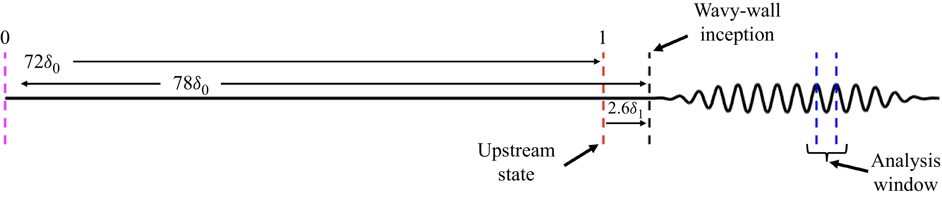

 2.6δ1
 δ1∗
 θ1∗
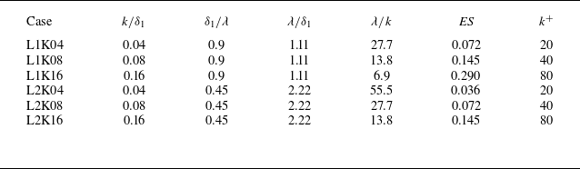


 x/δ1≈36
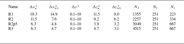
 u
 wv

 u+=y+
 u+=(1/κ)ln(y+)+5.1
 urms+
 vrms+
 wrms+
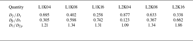
 f
 p
 Dt=Df+Dp
 Dfp

 Pw
 τw,x
 y/k
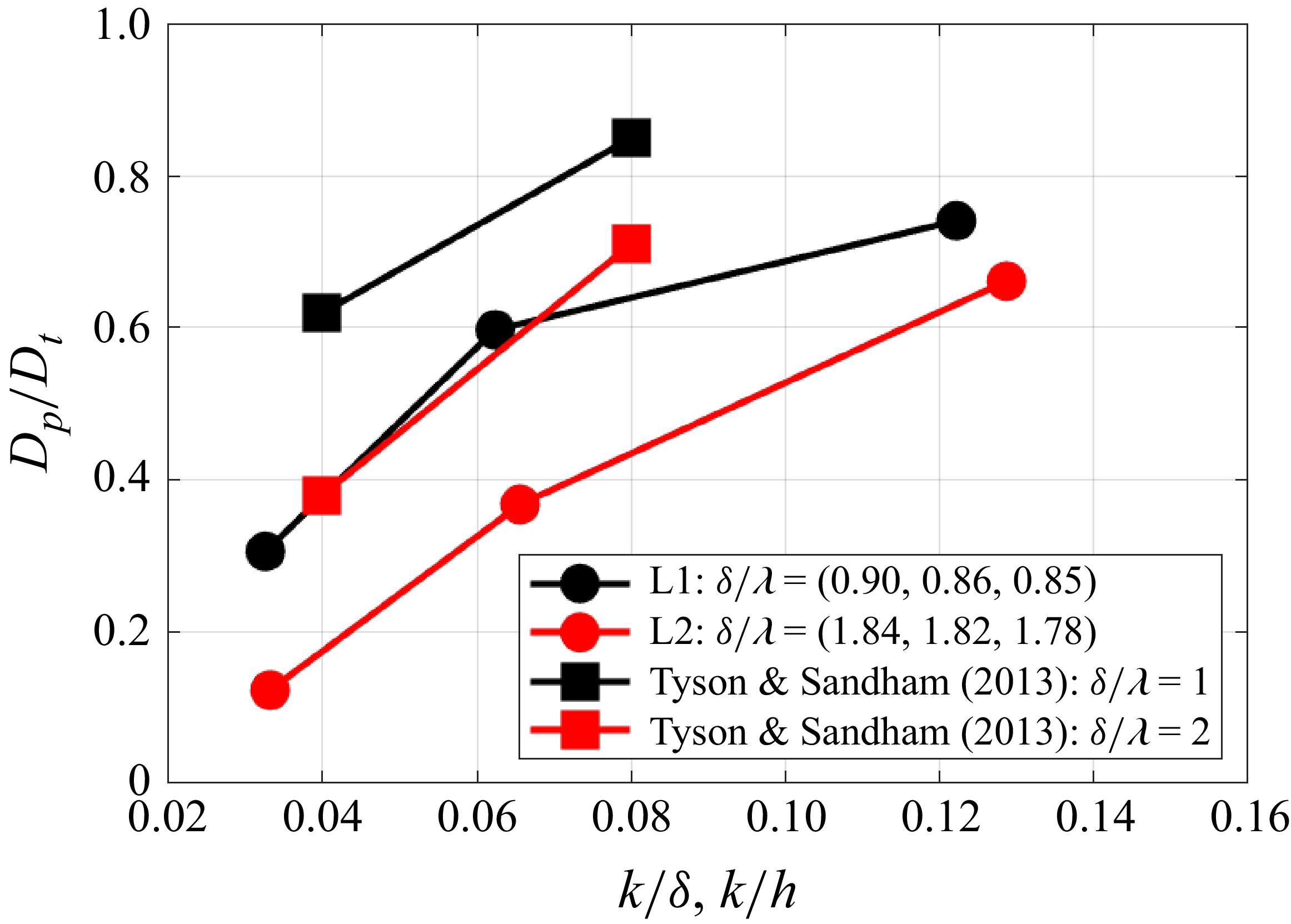
 Dp
 Dt
 h
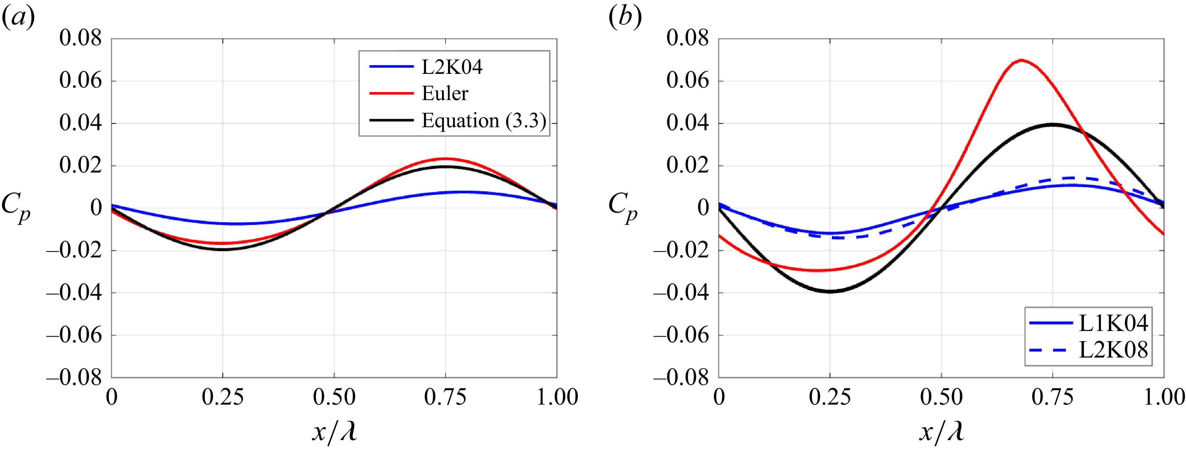
 Cp

 2y/k

 u~=0


 ρwuτ3/δν

 ρwuτ3/δν

 Pw,rms′
 Pw,rms′
 τw,rms′
 τw,rms′
 Pw,rms′
 Df
 Pw,rms′
 Dt

 Pw,rms′

 Pw,rms′2
 StL=0.03,0.1,0.5,1.0

 x/λ=0
 x/λ=0.25
 x/λ=0.5
 x/λ=0.75

 uτ=Dt/⟨ρ¯w⟩

 Q
 ωx

 τw,z

 Pw′>Pw,rms,u′
 τw′>τw,rms,u′


 GT

 τw,x¯
 P¯w
 q¯w
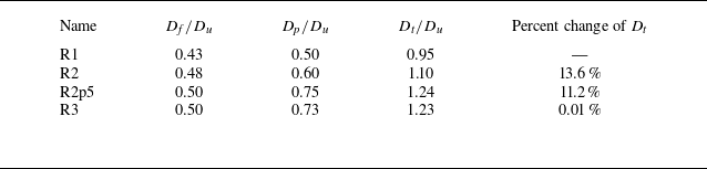
 f
 p
 Dt=Df+Dp
 Du

 x/λ=0.75


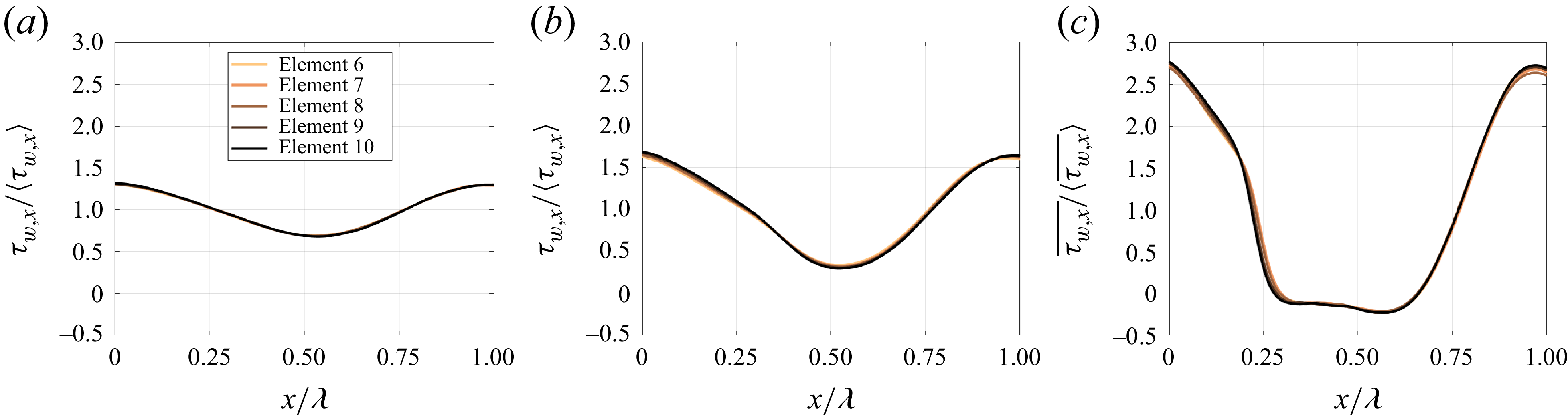
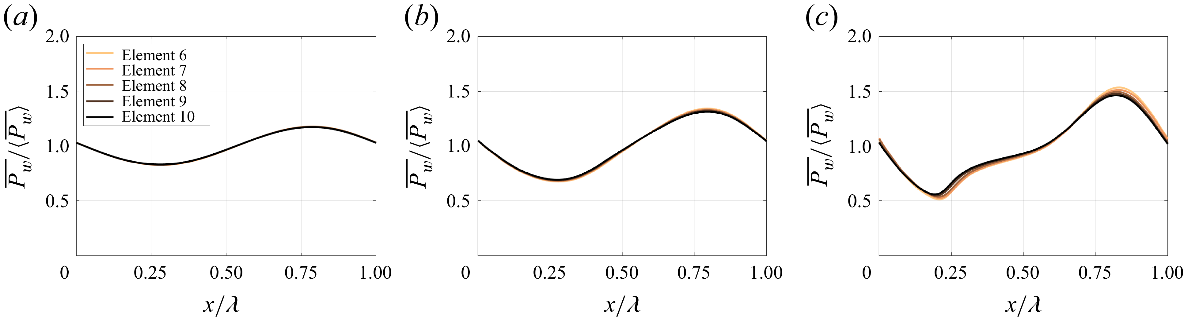
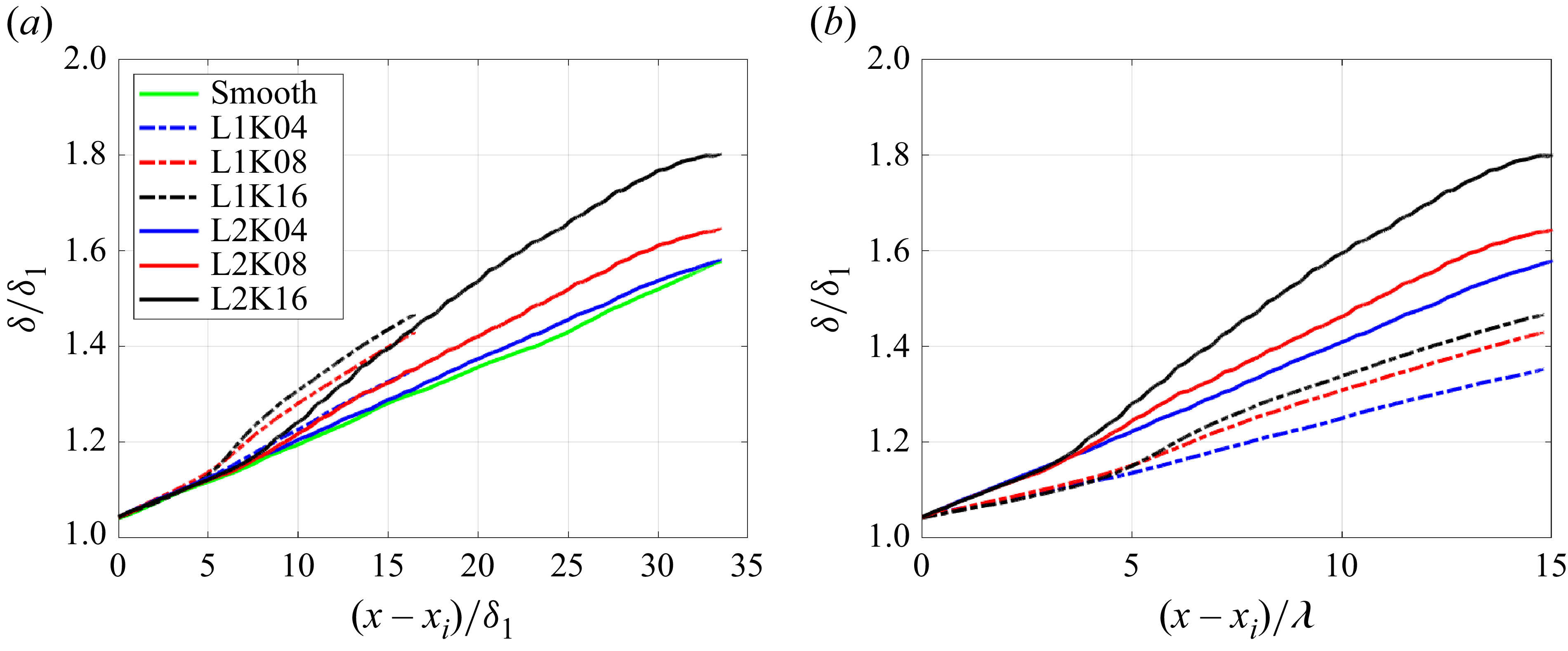
 xi


