1. Introduction
While premixed turbulent combustion has been utilized widely over the past century, the physics of this multiscale and highly nonlinear phenomenon requires a substantially deeper understanding, and the predictive capabilities of available models are still limited (Bilger et al. Reference Bilger, Pope, Bray and Driscoll2005; Poinsot & Veynante Reference Poinsot and Veynante2005; Lipatnikov Reference Lipatnikov2012). Although various approaches to theoretical, phenomenological, Reynolds-averaged Navier–Stokes (RANS) or large eddy simulation (LES) research into turbulent flames have been developed, they either address a hypothetical problem that cannot be investigated experimentally, e.g. many models deal with an unbounded statistically stationary planar 1D flame that propagates in homogeneous, isotropic and statistically stationary turbulence, or invoke closure relations obtained by considering such a hypothetical problem. Even if results yielded by a combustion model can be used in RANS or LES study of a laboratory flame, it is very difficult to judge what particular simplifications are responsible for eventual disagreement between measured and computed data when testing the model against experiments. For instance, a model that is rigorous under invoked simplifications could fail in predicting experimental data, because a single simplification is wrong, whereas a model that invokes the same simplifications plus a wrong one could match the same measured data if two wrong simplifications counterbalance one another.
From this perspective, direct numerical simulation (DNS) of a turbulent reacting flow appears to be a unique tool for basic research, because, in contrast to an experiment, a DNS study can deal with a problem that is addressed by a model to be investigated. For instance, 3D DNS of premixed turbulent burning in the case of a single global reaction can be used straightforwardly to test and rank models that do not allow for complex combustion chemistry, but take into account density variations and a finite thickness of the instantaneous heat-release zone. In order to straightforwardly assess models developed by neglecting the thickness of the heat-release zone, DNS can address self-propagation of an infinitely thin interface. Direct numerical simulations performed in a constant-density case allow one to investigate models that neglect the influence of heat release on the flow. Thus, while the leading research groups have succeeded already in 3D DNS of highly turbulent premixed flames by allowing for density variations and complex combustion chemistry (Chen Reference Chen2011; Aspden, Day & Bell Reference Aspden, Day and Bell2015; Carlsson, Yu & Bai Reference Carlsson, Yu and Bai2015; Yenerdag et al. Reference Yenerdag, Fukushima, Shimura, Tanahashi and Miyauchi2015) and advanced towards DNS of laboratory flames (Day et al. Reference Day, Tachibana, Bell, Lijewski, Beckner and Cheng2012), DNS studies of substantially simplified problems appear to be of great basic interest and importance in order to straightforwardly assess various theories or models used, e.g., in RANS or LES applications.
Even if we consider the simplest case of self-propagation of an interface in a constant-density turbulent flow, the problem is still of basic interest for a number of reasons. First, models developed under such simplifications are still cornerstones for many phenomenological, RANS or LES studies of premixed turbulent combustion, with different models yielding different results. For instance, starting from the pioneering work by Damköhler (Reference Damköhler1940) and Shchelkin (Reference Shchelkin1947), many papers have aimed at modelling the speed
 $S_{T,\infty }$
of a statistically stationary planar 1D premixed turbulent flame in the limit case of a constant density and infinitely thin instantaneous flame front, e.g. see a study by Zimont & Pagnini (Reference Zimont and Pagnini2011) as a recent example. Such models result typically in
 $$\begin{eqnarray}S_{T,\infty }=S_{L}\,f(U^{\prime }/S_{L}),\end{eqnarray}$$
where
 $S_{L}$
is the laminar flame speed and
 $U^{\prime }$
is the r.m.s. turbulent velocity. This expression is often substantiated with dimensional reasoning, because
 $S_{L}$
is the sole mixture characteristic that can affect
 $S_{T,\infty }$
in this hypothetical case (the laminar flame thickness
 ${\it\delta}_{L}\rightarrow 0$
and the density ratio
 ${\it\sigma}={\it\rho}_{u}/{\it\rho}_{b}=1$
, where subscripts
 $u$
and
 $b$
designate unburned and burned mixture respectively). Even if such a substantiation can be disputed by highlighting the primary contribution of small-scale eddies to an increase in a surface area in the Kolmogorov turbulence (Batchelor Reference Batchelor1952), the present authors are not aware of another type of expression for
 $S_{T,\infty }$
obtained in the case of
 ${\it\delta}_{L}\rightarrow 0$
and
 ${\it\sigma}=1$
.
Almost all known versions of (1.1) are subsumed by the following expression (Damköhler Reference Damköhler1940; Shchelkin Reference Shchelkin1947; Pocheau Reference Pocheau1994; Zimont & Pagnini Reference Zimont and Pagnini2011):
 $$\begin{eqnarray}S_{T,\infty }=(aS_{L}^{q}+b{U^{\prime }}^{q})^{1/q},\end{eqnarray}$$
while Yakhot (Reference Yakhot1988) has derived another expression,
 $$\begin{eqnarray}\frac{S_{T,\infty }}{S_{L}}=\exp \left(\frac{{U^{\prime }}^{2}}{S_{T,\infty }^{2}}\right),\end{eqnarray}$$
using renormalization group technique. Various models yield various values of the constant
 $b$
and power exponent
 $q$
in (1.2), whereas the constant
 $a$
is typically equal to unity in order for
 $S_{T,\infty }(U^{\prime }\rightarrow 0)\rightarrow S_{L}$
. While neither (1.2) nor (1.3) holds at
 $S_{L}=0$
, e.g. (1.2) yields
 $S_{T,\infty }=O(U^{\prime })>0$
at
 $S_{L}=0$
, a constraint that the dependence of
 $S_{T,\infty }$
on
 $S_{L}$
is continuous at
 $S_{L}=0$
does not seem to be necessary. As pointed out by a reviewer, such a ‘propagation’ anomaly ‘is somewhat but not entirely analogous to the energy dissipation anomaly of turbulence’.
A DNS study of self-propagation of an interface in a constant-density turbulent flow offers a unique opportunity to straightforwardly assess models that result in (1.2) with various
 $q$
or (1.3), as well as RANS and/or LES approaches based on these models.
For completeness, it is worth noting the following basic issue, which is relevant to weakly turbulent (
 $U^{\prime }\ll S_{L}$
) flows and, therefore, is beyond the scope of the present study restricted to
 $0.5\leqslant U^{\prime }/S_{L}\leqslant 10$
. On the one hand, Clavin & Williams (Reference Clavin and Williams1979), Aldredge & Williams (Reference Aldredge and Williams1991) and Aldredge (Reference Aldredge2006) analysed the limit case of
 $U^{\prime }\ll S_{L}$
and arrived at
 $$\begin{eqnarray}\frac{S_{T,\infty }}{S_{L}}=1+C\left(\frac{U^{\prime }}{S_{L}}\right)^{q},\end{eqnarray}$$
with
 $q=2$
. The same asymptotic relation results from (1.3) at
 $U^{\prime }\ll S_{L}$
. It was also supported in numerical simulations (Ashurst & Sivashinsky Reference Ashurst and Sivashinsky1991; Cambray & Joulin Reference Cambray and Joulin1992; Akkerman & Bychkov Reference Akkerman and Bychkov2003; Creta & Matalon Reference Creta and Matalon2011; Fogla, Creta & Matalon Reference Fogla, Creta and Matalon2013) that dealt with velocity fields that reproduced certain features of turbulent flows. On the other hand, Kerstein & Ashurst (Reference Kerstein and Ashurst1992) argued that this scaling held during a limited time interval, whereas the steady state
 $q=4/3$
in random velocity fields. This result was also supported in numerical simulations (Kerstein & Ashurst Reference Kerstein and Ashurst1994) and was not disputed in a later analysis by Aldredge (Reference Aldredge2006). Recently, Mayo & Kerstein (Reference Mayo and Kerstein2007) reduced the problem of front propagation in a weakly turbulent isotropic medium to the inviscid Burgers equation subject to white-in-time noise and arrived at the steady state
 $q=4/3$
using rigorous mathematical results obtained for white noise that was ‘periodic in space with any given smooth correlation function’. This analysis was further supported by Mayo & Kerstein (Reference Mayo and Kerstein2008). Moreover, Mayo & Kerstein (Reference Mayo and Kerstein2007) argued that
 $q$
could be equal to 2 either during a short time interval before cusp formation or in a sufficiently anisotropic medium. As already noted above, this issue is beyond the scope of the present DNS study restricted to
 $0.5\leqslant U^{\prime }/S_{L}\leqslant 10$
.
Second, while the aforementioned models and the vast majority of other models place the focus of consideration on fully developed turbulent burning, flame development requires a long time and premixed turbulent combustion is typically the developing wave, as reviewed elsewhere (Prudnikov Reference Prudnikov and Raushenbakh1967; Lipatnikov & Chomiak Reference Lipatnikov and Chomiak2002; Lipatnikov Reference Lipatnikov2012). While the terms ‘statistically stationary’ and ‘fully developed’ flames are equivalent in the case of a statistically 1D turbulent flow, we will use the latter term in the rest of the paper, because a statistically stationary flame can develop if the flow is statistically 2D or 3D. For instance, if we consider statistically stationary combustion behind a stabilizer, turbulent flame development manifests itself in an increase in the mean flame brush thickness
 ${\it\delta}_{T}$
with the distance from the stabilizer, and this well-documented phenomenon is basically similar to the growth of a turbulent mixing layer (decay of grid-generated turbulence is another well-known example of a flow that develops in the statistically stationary case). In spite of the practical importance of turbulent flame development, only a few analytical expressions have so far been obtained to describe the dependence of the turbulent flame speed
 $S_{T}$
or mean flame brush thickness
 ${\it\delta}_{T}$
on the flame-development time (Scurlock & Grover Reference Scurlock and Grover1953; Prudnikov Reference Prudnikov and Raushenbakh1967; Kuznetsov Reference Kuznetsov1975; Peters Reference Peters2000; Lipatnikov & Chomiak Reference Lipatnikov and Chomiak2002; Lipatnikov Reference Lipatnikov2012), with all these models ignoring effects associated with density variations. Therefore, a DNS study of self-propagation of an interface in a constant-density turbulent flow offers an opportunity to investigate these models and to gain further insight into premixed turbulent flame development. It is worth noting that the terms ‘fully developed flame’ and ‘flame development’ should solely be considered in the statistical sense. For instance, a spatially or ensemble-averaged characteristic
 $\bar{q}$
of turbulent burning can vary with time
 $t$
in both developing and fully developed flames, but
 $\bar{q}(t)$
shows a clear trend in the former case, e.g. growth of turbulent flame speed or mean thickness, and exhibits oscillations in the latter case, even if the oscillation magnitude can be large (Poludnenko & Oran Reference Poludnenko and Oran2011; Lipatnikov et al.
Reference Lipatnikov, Chomiak, Sabelnikov, Nishiki and Hasegawa2015; Poludnenko Reference Poludnenko2015).
Third, in a premixed turbulent flame, the mean transport of a scalar quantity
 $q$
can occur not only in the direction opposite to
 $\boldsymbol{{\rm\nabla}}\bar{q}$
, as in many non-reacting flows, but also in the same direction, i.e.
 $\overline{\boldsymbol{u}^{\prime }q^{\prime }}\boldsymbol{\cdot }\boldsymbol{{\rm\nabla}}\bar{q}>0$
. Here,
 $\boldsymbol{u}$
is the flow velocity vector, overlines and overbars designate the Reynolds average with
 $q^{\prime }=q-\bar{q}$
. This phenomenon, known as countergradient transport, was theoretically predicted by Clavin & Williams (Reference Clavin and Williams1979) and Libby & Bray (Reference Libby and Bray1981), was experimentally discovered by Moss (Reference Moss1980) and Yanagi & Mimura (Reference Yanagi and Mimura1981), and was documented in a number of subsequent measurements and DNS studies reviewed elsewhere (Bray Reference Bray1995; Lipatnikov & Chomiak Reference Lipatnikov and Chomiak2010; Robin, Mura & Champion Reference Robin, Mura and Champion2011). Countergradient transport is often attributed to a faster (slower) acceleration of hot and light products (cold and heavy fresh gas) by a combustion-induced pressure gradient (Libby & Bray Reference Libby and Bray1981), i.e. the difference between turbulent transport in premixed flames and mixing layers is commonly associated with density variations in flames. However, as argued by Corrsin (Reference Corrsin1974), chemical reactions can also affect turbulent transport independently of density variations, e.g. if
 ${\it\sigma}=1$
. The present authors are aware of a single model aimed at allowing straightforwardly for such effects in premixed turbulent flames (Borghi & Dutoya Reference Borghi and Dutoya1978), and the issue definitely requires further study. Moreover, it is unclear whether or not chemical reactions can substantially affect turbulent transport if they are localized to a zone of vanishing thickness, i.e.
 ${\it\delta}_{L}\rightarrow 0$
. A DNS study of self-propagation of an interface in a constant-density turbulent flow offers an opportunity to gain an insight into these issues, because neither density variations nor combustion-induced pressure gradient affect turbulent transport in that simple case.
Fourth, various models developed to evaluate turbulent flame speed or mean rate
 $\overline{W}$
of product creation within the premixed turbulent flame brush (Williams Reference Williams1985; Peters Reference Peters2000; Lipatnikov & Chomiak Reference Lipatnikov and Chomiak2002; Veynante & Vervisch Reference Veynante and Vervisch2002; Poinsot & Veynante Reference Poinsot and Veynante2005; Lipatnikov Reference Lipatnikov2012) consider
 $U^{\prime }$
to be the primary characteristic of turbulence, e.g. see (1.1)–(1.4). Accordingly, variations in
 $U^{\prime }$
within turbulent flames should be taken into account in order for an RANS or LES approach to be able to predict key characteristics of premixed turbulent combustion. However, as argued elsewhere (Lipatnikov Reference Lipatnikov2009a
; Lipatnikov & Chomiak Reference Lipatnikov and Chomiak2010), a consistent definition of
 $U^{\prime }$
in a premixed turbulent flame is an issue. It can be revealed, e.g., by considering the case of fresh reactants and burned products separated by an infinitely thin self-propagating front (flamelet). In this case (Bray, Libby & Moss Reference Bray, Libby and Moss1985),
 $$\begin{eqnarray}\displaystyle \frac{\overline{{\it\rho}u_{k}^{\prime \prime }u_{k}^{\prime \prime }}}{\bar{{\it\rho}}} & = & \displaystyle (1-\tilde{c})(\overline{u_{k}^{\prime }u_{k}^{\prime }})_{u}+\tilde{c}(\overline{u_{k}^{\prime }u_{k}^{\prime }})_{b}+\tilde{c}(1-\tilde{c})(\bar{u}_{k,b}-\bar{u}_{k,u})(\bar{u}_{k,b}-\bar{u}_{k,u})\nonumber\\ \displaystyle & = & \displaystyle (1-\tilde{c})(\overline{u_{k}^{\prime }u_{k}^{\prime }})_{u}+\tilde{c}(\overline{u_{k}^{\prime }u_{k}^{\prime }})_{b}+\frac{\overline{{\it\rho}u_{k}^{\prime \prime }c^{\prime \prime }}~\overline{{\it\rho}u_{k}^{\prime \prime }c^{\prime \prime }}}{\bar{{\it\rho}}^{2}\tilde{c}(1-\tilde{c})},\end{eqnarray}$$
i.e. the r.m.s. velocity
 $U^{\prime }=(\overline{{\it\rho}u_{k}^{\prime \prime }u_{k}^{\prime \prime }}/3\bar{{\it\rho}})^{1/2}$
defined in a standard (for non-reacting constant-density flows) manner is straightforwardly affected by the magnitude of the slip velocity vector
 ${\rm\Delta}\boldsymbol{u}=\bar{\boldsymbol{u}}_{b}-\bar{\boldsymbol{u}}_{u}$
and, therefore, depends not only on the turbulence, but also on the velocity jump across the flamelet. Here,
 ${\it\rho}$
is the density,
 $c$
is the combustion progress variable,
 $(\overline{u_{k}^{\prime }u_{k}^{\prime }})_{u}$
and
 $(\overline{u_{k}^{\prime }u_{k}^{\prime }})_{b}$
are the traces of the Reynolds-stress tensors
 $(\overline{u_{i}^{\prime }u_{j}^{\prime }})_{u}=(\overline{u_{i}u_{j}})_{u}-\bar{u}_{i,u}\bar{u}_{j,u}$
and
 $(\overline{u_{i}^{\prime }u_{j}^{\prime }})_{b}=(\overline{u_{i}u_{j}})_{b}-\bar{u}_{i,b}\bar{u}_{j,b}$
conditioned on unburned and burned gas respectively,
 $\tilde{q}=\overline{{\it\rho}q}/\bar{{\it\rho}}$
designates the Favre (mass-weighted) average of any quantity
 $q$
with
 $q^{\prime \prime }=q-\tilde{q}$
, and the summation convention applies for the repeated index
 $k$
.
Alternatively, the conditioned r.m.s. velocity
 $U_{u}^{\prime }=(\overline{u_{k}^{\prime }u_{k}^{\prime }})_{u}/3$
or
 $U_{b}^{\prime }=(\overline{u_{k}^{\prime }u_{k}^{\prime }})_{b}/3$
has often been considered to be the true turbulence characteristic. However, substantial basic differences between the conditioned and the true r.m.s. turbulent velocities were recently highlighted by studying a set of very simple model problems (Lipatnikov Reference Lipatnikov2009a
). For instance, application of (1.5) to the case of equal densities of products and fresh mixture shows that
 $(\overline{u_{k}^{\prime }u_{k}^{\prime }})_{u}$
or
 $(\overline{u_{k}^{\prime }u_{k}^{\prime }})_{b}$
differs from
 $\overline{u_{k}^{\prime }u_{k}^{\prime }}$
due to the positive last term on the right-hand side, but it is
 $\overline{u_{k}^{\prime }u_{k}^{\prime }}$
that is the true turbulence characteristic in this case, because a self-propagating interface does not affect the velocity field when the density and viscosity are constants.
The basic difference between conditioned and canonical mean turbulence characteristics stems from the fact that conditional averaging is performed over a spatial domain whose boundary is wrinkled and randomly moves, with this motion being anisotropic. Due to the motion of the boundary, first, conditional averaging commutes neither with time nor with spatial derivatives, e.g. the divergence of the conditioned velocity vector does not vanish in a constant-density flow in a general case (Libby Reference Libby1975). Second, due to the flux of a fluid through the boundary, e.g. conversion of reactants to products in flamelets, conditioned balance equations involve source or sink terms that do not appear in the counterpart Reynolds-averaged equations. This point was clearly shown in the pioneering papers by Libby (Reference Libby1975) and Dopazo (Reference Dopazo1977), who introduced conditioned balance equations into fluid mechanics in order to address external intermittency in constant-density turbulent flows. As far as the propagation of a flamelet of a finite thickness in a turbulent flow is concerned, proper conditioned balance equations were straightforwardly derived, e.g., by Lipatnikov (Reference Lipatnikov2008), see also equations (215)–(220) in a recent review paper by Lipatnikov & Chomiak (Reference Lipatnikov and Chomiak2010). One can easily show that these equations involve source or sink terms that do not vanish even in the constant-density case, e.g. see equations (2)–(4), (12) and (13) analysed by Lipatnikov (Reference Lipatnikov2011). These source/sink terms substantially change conditioned quantities when compared with the counterpart canonical Reynolds-averaged quantities.
Target-directed research into differences between the mean and conditioned r.m.s. velocities due to differences between the conventional and conditional averaging techniques has been scarce in the combustion literature to date. Recently, Lipatnikov (Reference Lipatnikov2011) stressed these differences by applying conditioned balance equations to numerical simulations of a statistically planar 1D premixed turbulent constant-density ‘flame’. However, the obtained results cannot be considered to be decisive proof due to a number of closure assumptions invoked. Experimental research into the discussed problem requires the knowledge of the true turbulence characteristics within a premixed flame brush, but such characteristics have not yet been defined in a consistent manner in a general case. While they are confidently known in a constant-density case, it cannot be studied in a combustion experiment. On the contrary, DNS of propagation of an interface in a constant-density turbulent flow is well suited for gaining further insight into the relation between conditioned and true turbulence characteristics. Indeed, first, conditioned quantities are best defined in the case of an infinitely thin front. Second, turbulence characteristics are well defined in the constant-density flow and can be used as reference quantities.
Thus, a DNS study of self-propagation of an interface in constant-density turbulence offers an opportunity to investigate a number of basic issues relevant to an understanding of and modelling of premixed turbulent combustion, such as (i) global characteristics of the fully developed mean front, (ii) development of the global front characteristics, (iii) influence of interface propagation on turbulent transport of a scalar that characterizes the state of the fluid (before or behind the interface) and (iv) differences between conditioned and true turbulence characteristics. The present work aims at addressing these issues. It continues a recent DNS study (Yu, Lipatnikov & Bai Reference Yu, Lipatnikov and Bai2014), whose focus was mainly placed on issues (iii), (iv) and, in part, (i), with them being solely addressed in the case of fully developed mean fronts. In addition to investigating turbulent front development and much more detailed discussion of issue (i), the present work covers wider ranges of both
 $U^{\prime }/S_{L}$
and turbulent Reynolds numbers.
In the premixed turbulent combustion literature, the vast majority of DNS papers deal with a front of a finite thickness, while self-propagation of an interface in constant-density homogeneous isotropic turbulence is also addressed (Kerstein, Ashurst & Williams Reference Kerstein, Ashurst and Williams1988; Yeung, Girimaji & Pope Reference Yeung, Girimaji and Pope1990; Girimaji & Pope Reference Girimaji and Pope1992; Wenzel & Peters Reference Wenzel and Peters2000, Reference Wenzel and Peters2005; Treurniet, Nieuwstadt & Boersma Reference Treurniet, Nieuwstadt and Boersma2006; Creta & Matalon Reference Creta and Matalon2011; Fogla et al.
Reference Fogla, Creta and Matalon2013; Shin & Lieuwen Reference Shin and Lieuwen2013). In some of these simulations, the influence of thermal expansion on the flow and/or the influence of turbulent stretch rates on the front speed was taken into account. For instance, Wenzel & Peters (Reference Wenzel and Peters2005) allowed for variations in
 $S_{L}$
due to local front curvature in intense turbulence (
 $U^{\prime }/S_{L}=2.1{-}17.1$
, but
 $\mathit{Re}=78$
). Moreover, Wenzel & Peters (Reference Wenzel and Peters2000) investigated the influence of the density ratio on the mean front characteristics at a low
 $\mathit{Re}=34$
and a high
 $U^{\prime }/S_{L}=15.9$
. When those simulations were run in the case of a constant density and a constant
 $S_{L}$
, the ratio of
 $U^{\prime }/S_{L}$
was lower, i.e.
 $0.53<U^{\prime }/S_{L}\leqslant 2.1$
(Wenzel & Peters Reference Wenzel and Peters2000, Reference Wenzel and Peters2005). Treurniet et al. (Reference Treurniet, Nieuwstadt and Boersma2006) used a constant
 $S_{L}$
, but varied the density ratio at
 $U^{\prime }/S_{L}=O(1)$
. In the 2D simulations of weakly turbulent combustion by Creta & Matalon (Reference Creta and Matalon2011) and Fogla et al. (Reference Fogla, Creta and Matalon2013), thermal expansion effects were taken into account and
 $S_{L}$
depended linearly on the local stretch rate, with the Markstein number being positive. However, the aforementioned issues (ii)–(iv) were beyond the scope of the cited papers.
It is also worth noting that while consideration of burning in a statistically planar 1D flow is typical for DNS research into premixed turbulent combustion, some important physical mechanisms cannot be investigated under such conditions, e.g. effects associated with the mean flow tangential to the flame brush (Philips Reference Philips1972; Hemchandra & Lieuwen Reference Hemchandra and Lieuwen2010; Amato & Lieuwen Reference Amato and Lieuwen2014), the mean curvature of the flame brush (Lipatnikov & Chomiak Reference Lipatnikov and Chomiak2007; Shin & Lieuwen Reference Shin and Lieuwen2013) or the interaction between two mutually inclined mean flames (Troiani, Battista & Picano Reference Troiani, Battista and Picano2013).
The present paper is organized as follows. In the next section, the governing equations are briefly summarized. Direct numerical simulation attributes are reported in § 3. The obtained results are discussed in § 4 followed by conclusions.
In order to stress the difference between constant-density turbulent flow and turbulent burning accompanied by significant density variations, we will avoid the terms flame and flamelet when discussing self-propagating interfaces in the rest of the paper. The statistically planar spatial region that envelops all wrinkled interfaces at a single instant will be called the mean front. However, because the present study aims at clarifying basic issues associated with premixed turbulent combustion, the terms ‘turbulent flame speed’
 $S_{T}$
, ‘mean flame brush thickness’
 ${\it\delta}_{T}$
and ‘flame development’ will be applied to the speed and thickness of the mean front and to its development respectively. Moreover, fluid before and behind the interface will be called ‘unburned’ and ‘burned’ mixture and will be designated using subscripts
 $u$
and
 $b$
respectively. Furthermore, the speed of the self-propagation of the interface will be designated with the symbol
 $S_{L}$
, which is associated with the laminar flame speed in the combustion literature. Finally, we will use the word ‘flame’ when comparing the present DNS data with various models of premixed turbulent combustion. All of these reservations are worth bearing in mind when reading ‘flame’ in the rest of the paper.
2. Governing equations
Constant-density turbulent flow is governed by the Navier–Stokes equations
 $$\begin{eqnarray}\displaystyle & \displaystyle \frac{\partial u_{k}}{\partial x_{k}}=0, & \displaystyle\end{eqnarray}$$
 $$\begin{eqnarray}\displaystyle & \displaystyle \frac{\partial u_{i}}{\partial t}+u_{k}\frac{\partial u_{i}}{\partial x_{k}}=-\frac{\partial p}{\partial x_{i}}+{\it\nu}\frac{\partial ^{2}u_{i}}{\partial x_{k}^{2}}+\,f_{i}, & \displaystyle\end{eqnarray}$$
 ${\it\nu}$
and
 $p$
are the kinematic viscosity and pressure respectively, and the term
 $f_{i}(\boldsymbol{x},t)$
is added in order to maintain constant turbulence intensity by using energy forcing at low wavenumbers. Under such forcing, the injected energy cascades down to balance the dissipation at small scales, with the turbulence statistics at smaller scales being hardly affected (Siggia Reference Siggia1981). The forcing scheme is discussed further in the next section.
Self-propagation of an interface is simulated by numerically solving the level-set equation (Williams Reference Williams1985; Kerstein et al. Reference Kerstein, Ashurst and Williams1988; Peters Reference Peters2000)
 $$\begin{eqnarray}\frac{\partial G}{\partial t}+\boldsymbol{u}\boldsymbol{\cdot }\boldsymbol{{\rm\nabla}}G=S_{L}|\boldsymbol{{\rm\nabla}}G|,\end{eqnarray}$$
where
 $G$
is a signed distance function to the closest interface associated with
 $G(\boldsymbol{x},t)=0$
. The combustion progress variable
 $c(\boldsymbol{x},t)=H[G(\boldsymbol{x},t)]$
is defined using the Heaviside function
 $H(z)$
. The interface speed
 $S_{L}$
is kept constant. As far as the relevance of such an assumption to premixed combustion is concerned, the case of
 $S_{L}=\text{const.}$
is associated with a laminar flame characterized by a zero Markstein number
 $\mathit{Ma}$
with respect to unburned gas, e.g. a near-stoichiometric methane–air flame. It is worth also noting that theories of weakly perturbed laminar flames predict that variously defined Markstein numbers depend on the density ratio and Lewis number
 $\mathit{Le}$
, with
 $\mathit{Ma}$
vanishing in the constant-density equidiffusive (
 $\mathit{Le}=1$
) case (Clavin Reference Clavin1985). Because these theories yield
 $S_{L}=\text{const.}$
for an infinitely thin flame, the present study of an interface that propagates at a constant speed is consistent with them.
3. Numerical method and running conditions
Simulations were performed using a simplified in-house DNS solver (Yu, Yu & Bai Reference Yu, Yu and Bai2012) developed for low Mach number reacting flows with detailed chemistry and already applied to various reacting flow systems (Zhang, Yu & Bai Reference Zhang, Yu and Bai2012; Yu & Bai Reference Yu and Bai2013a ; Yu et al. Reference Yu, Yu, Fan, Christensen, Konnov and Bai2013; Carlsson, Yu & Bai Reference Carlsson, Yu and Bai2014). The temporal integration of the governing equations is based on a second-order symmetrical Strang splitting algorithm, originally designed to accommodate a standalone chemistry solver. With one global time step, the integration of viscous terms is split into multiple sub-time steps of explicit integrations, with the substep size given by the diffusion stability limit. The spatial discretization and interpolations are based on sixth-order centre schemes. The Poisson equation for pressure is solved with an efficient multigrid method (Yu & Bai Reference Yu and Bai2013b ). The DNS code is implemented in a vector form enabling 1D, 2D and 3D simulations.
The computational domain is a rectangular box of size
 $L_{x}\times L_{y}\times L_{z}$
, with
 $L_{x}=4L_{y}=4L_{z}=4L$
, discretized on a uniform grid of
 $N_{x}\times N_{y}\times N_{z}$
cells, with
 $N_{x}=4N_{y}=4N_{z}$
. The initial turbulence field is generated by synthesizing prescribed Fourier waves (Yu & Bai Reference Yu and Bai2014) with an initial r.m.s. velocity
 $U_{0}^{\prime }$
and integral length scale
 ${\it\Lambda}_{0}=L/4$
. Following Ghosal et al. (Reference Ghosal, Lund, Moin and Akselvoll1995), the forcing function
 $\boldsymbol{f}(\boldsymbol{x},t)=\sum _{{\bf\kappa}}\hat{\boldsymbol{f}}_{{\bf\kappa}}(t)\exp (-\text{i}{\bf\kappa}\boldsymbol{\cdot }\boldsymbol{x})$
, with
 $$\begin{eqnarray}\hat{\boldsymbol{f}}_{{\bf\kappa}}(t)=\langle {\it\varepsilon}\rangle \frac{\hat{\boldsymbol{u}}_{{\bf\kappa}}(t)1_{{\bf\kappa}-{\bf\kappa}_{t}(t)}}{\hat{\boldsymbol{u}}_{{\bf\kappa}}(t)\boldsymbol{\cdot }\hat{\boldsymbol{u}}_{{\bf\kappa}}^{\ast }(t)},\end{eqnarray}$$
is invoked in order to maintain statically stationary turbulence. Here,
 $\hat{\boldsymbol{f}}_{{\bf\kappa}}$
is the Fourier mode of
 $\boldsymbol{f}$
in the wavenumber
 ${\bf\kappa}$
-space,
 $$\begin{eqnarray}{\it\varepsilon}=2{\it\nu}S_{ij}S_{ij}=\frac{{\it\nu}}{2}\left(\frac{\partial u_{i}}{\partial x_{j}}+\frac{\partial u_{j}}{\partial x_{i}}\right)\left(\frac{\partial u_{i}}{\partial x_{j}}+\frac{\partial u_{j}}{\partial x_{i}}\right)\end{eqnarray}$$
is the dissipation rate, the bracket
 $\langle \cdot \rangle$
designates averaging over entire domain. The caret operator designates the complex Fourier mode
 $\hat{q}_{{\bf\kappa}}(t)=\langle q(\boldsymbol{x},t)\exp (-\text{i}{\bf\kappa}\boldsymbol{\cdot }\boldsymbol{x})\rangle$
for any
 $q,1_{{\bf\kappa}-{\bf\kappa}_{r}}=1$
when
 ${\bf\kappa}={\bf\kappa}_{r}$
, otherwise 0, and
 ${\bf\kappa}_{r}=\boldsymbol{m}k_{0}$
is a randomly selected (at each time step) non-zero wavenumber vector within a lower wavenumber band, i.e.
 $|{\bf\kappa}_{r}|\leqslant {\it\kappa}_{f}=3k_{0}=6{\rm\pi}/L$
, where
 $\boldsymbol{m}$
is a random integer vector. Figure 1(a) validates the above forcing strategy by showing that the r.m.s. velocity
 $U^{\prime }$
is maintained as the initial value, i.e.
 $U^{\prime }=U_{0}^{\prime }$
, while the normalized averaged dissipation rate
 $\langle {\it\varepsilon}\rangle {\it\Lambda}_{0}/{U_{0}^{\prime }}^{3}$
fluctuates slightly above
 $3/2$
after a short period (
 $t<{\it\tau}_{t}^{0}$
, where the initial turbulence eddy turnover time
 ${\it\tau}_{t}^{0}={\it\Lambda}_{0}/U^{\prime }$
) of rapid transition from the initial artificially synthesized flow to the fully developed turbulence. It was also shown in figure 2 in our previous work (Yu et al.
Reference Yu, Lipatnikov and Bai2014), where the same forcing method was applied, that the forced turbulence achieved good statistical homogeneity and isotropy over the entire domain, i.e.
 $\overline{u^{2}}=\overline{w^{2}}={U^{\prime }}^{2}$
,
 $\overline{uw}=0$
and
 $\overline{u^{3}}=0$
.
(a) Temporal evolution of the r.m.s. velocity
 $U^{\prime }$
(dashed line) and the domain-averaged normalized dissipation rate (solid line) in the case of
 $\mathit{Re}=200$
. (b) Turbulent energy spectrum
 $E(k)$
computed in cases of
 $\mathit{Re}=50$
, 100 and 200;
 $k$
is the wavenumber.

Fifteen 3D-DNS cases were simulated by varying the normalized interface speed
 $S_{L}/U^{\prime }$
(0.1, 0.2, 0.5, 1.0, 1.5 and 2.0) and the Reynolds number
 $\mathit{Re}=U^{\prime }{\it\Lambda}_{0}/{\it\nu}$
(50, 100 and 200), see table 1. In order to change the two parameters independently from one another,
 $S_{L}/U^{\prime }$
and
 $\mathit{Re}$
were varied by varying
 $S_{L}$
and
 ${\it\Lambda}_{0}=L/4$
respectively. At
 $\mathit{Re}=200$
, only three cases with
 $S_{L}/U^{\prime }=0.1$
, 1.0 and 2.0 were addressed. When comparing these conditions with the characteristics of typical premixed turbulent flames, a low ratio of
 $S_{L}/U^{\prime }=0.1$
appears to be inconsistent with reduction of combustion to the propagation of an interface. However, from the purely theoretical viewpoint, there is no inconsistency if
 ${\it\Lambda}/{\it\delta}_{L}\gg (U^{\prime }/S_{L})^{3}$
and, therefore, the Karlovitz number
 $Ka\propto (U^{\prime }/S_{L})^{3/2}({\it\Lambda}/{\it\delta}_{L})^{-1/2}\ll 1$
. At the Reynolds numbers reached in the present DNS study, the constraint of
 $Ka\ll 1$
does not hold if
 $S_{L}/U^{\prime }=0.1$
or 0.2, but, because the results reported in the following depend weakly on
 $\mathit{Re}$
, we could expect that they will be valid even at Reynolds numbers sufficiently high in order for
 $Ka\ll 1$
.
Fifteen DNS cases.

The Reynolds number was varied by adjusting the domain size
 $L$
while keeping the domain aspect ratio fixed. The largest grid was used in the case of
 $\mathit{Re}=200$
. In all cases, the grid cell size
 ${\rm\Delta}x=L_{x}/N_{x}=L_{y}/N_{y}=L_{z}/N_{z}$
was uniform and the computational time step was set as
 ${\rm\Delta}t=0.029{\rm\Delta}x/U^{\prime }$
. Because interface propagation does not influence the flow in the case of constant
 ${\it\rho}$
and
 ${\it\nu}$
, the flow statistics were the same in all cases that had different
 $S_{L}$
but the same
 $\mathit{Re}$
. Table 2 shows the turbulence characteristics computed at various
 $\mathit{Re}$
. These characteristics were calculated after the forced turbulence reached statistical stationarity, i.e. at
 $t>5{\it\tau}_{t}^{0}$
. The integral length scale
 ${\it\Lambda}$
of the forced turbulence drifted away from the initially imposed value
 ${\it\Lambda}_{0}=L/4$
, with the ratio of
 ${\it\Lambda}/L$
being decreased when increasing
 $\mathit{Re}$
. A similar trend was reported by Eswaran & Pope (Reference Eswaran and Pope1988). The fully developed forced turbulence can be characterized by
 $\mathit{Re}_{t}=U^{\prime }{\it\Lambda}/{\it\nu}$
. Table 2 shows that
 $\mathit{Re}_{t}$
differed from, but remained close to, the initial
 $\mathit{Re}$
, which will be used for case references in the rest of the paper. The Kolmogorov scale
 ${\it\eta}=({\it\nu}^{3}/\overline{\langle {\it\varepsilon}\rangle })^{1/4}$
was of the order of the grid cell size
 ${\rm\Delta}x$
, indicating sufficient grid resolution. Here,
 $\overline{\langle {\it\varepsilon}\rangle }$
is the dissipation rate averaged over both the computational domain and time. The eddy turnover time
 ${\it\tau}_{t}={\it\Lambda}/U^{\prime }$
for the forced turbulence differed slightly from its initial value
 ${\it\tau}_{t}^{0}$
. Turbulence energy spectra
 $E(k)$
, computed by assuming the homogeneity and isotropy of the flow from DNS velocity fields picked randomly at
 $t>5{\it\tau}_{t}^{0}$
, are shown in figure 1(b) for all three
 $\mathit{Re}$
. The
 $-5/3$
spectrum is approached with an increase in
 $\mathit{Re}$
.
Mean flow characteristics of forcing maintained turbulence.

After the forced turbulence reached statistical stationarity, transient simulations of interface propagation were started by simultaneously releasing
 $M$
independent fields of
 $G_{m}^{T}$
(
 $m=1,\dots ,M=30$
; superscript
 $T$
means transient, as will be discussed later), with each interface
 $G_{m}^{T}=0$
being released as a
 $y$
–
 $z$
plane at
 $x=L_{x}(2m-1)/(2M)$
. Accordingly,
 $G_{m}^{T}[x=L_{x}(2m-1)/(2M),y,z,t=0]=0$
and
 $G_{m}^{T}(x,y,z,0)=x-L_{x}(2m-1)/(2M)$
within a narrow (six-cell) band that covered the
 $G_{m}^{T}=0$
interface.
Subsequently, the evolution of each
 $G_{m}^{T}$
field was simulated by numerically solving (2.3) within the narrow band (Wang Reference Wang2005), followed by reinitialization (
 $|\boldsymbol{{\rm\nabla}}G|=1$
) in order for the surrounding
 $G_{m}^{T}$
to be a signed distance function. A third-order weighted essential non-oscillating scheme (Jiang & Peng Reference Jiang and Peng2000) and a third-order total variation diminishing type Runge–Kutta scheme (Gottlieb & Shu Reference Gottlieb and Shu1998) were used for discretizing (2.3) spatially and temporally respectively.
In order for the zero level set obtained after the reinitialization to coincide with the original one, an improved sub-cell-fix reinitialization algorithm (Sun, Wang & Bai Reference Sun, Wang and Bai2010) was used in this work. The method is largely based on the sub-cell-fix scheme by Russo & Smereka (Reference Russo and Smereka2000), in which the signed distance function is first calculated using a ‘fixing’ algorithm for a subset of cells adjacent to the zero level set, while the redistancing algorithm by Sussman, Smereka & Osher (Reference Sussman, Smereka and Osher1994) is applied to other cells inside the narrow band.
The adopted level-set solver was described in detail by Sun et al. (Reference Sun, Wang and Bai2010). In particular, the grid dependence of the numerical solution was investigated and the adopted sub-cell-fix reinitialization method was shown to maintain spatial accuracy of the second order, e.g. see figure 12 in the cited paper. Moreover, the overall performance of the level-set solver was demonstrated in several challenging test cases, e.g. (i) a rotating slot disk, (ii) a circle that self-propagated at a speed that varied in space and time, and (iii) coalescing and segregating spheres. Furthermore, the adopted level-set scheme was shown to be capable of handling large local curvature of the surface.
The transient simulations were run over
 $2{\it\tau}_{t}^{0}$
before being reset. Then, the process was repeated. At the reset instants, the
 $G_{m}^{T}$
fields in the vicinity of each planar interface
 $x_{m}=L_{x}(2m-1)/(2M)$
were set equal to
 $x-x_{m}$
. Tracking of
 $M$
interfaces increased the sampling counts for computing the transient statistics.
Moreover, an additional long-living
 $G^{S}$
field was simulated to provide statistics for the fully developed turbulent front propagation. The
 $G^{S}=0$
planar interface was initially (
 $t=0$
) released at
 $x=L_{x}/2$
and propagated freely with no reset, in contrast to the transient interfaces. The long-living interface was covered by its own narrow band, which was independent of the 30 transient narrow bands. Calculations of fully developed front statistics began at
 $t=5{\it\tau}_{t}^{0}$
, with sampling every
 $100{\rm\Delta}t$
. In all DNS cases, the total sampling duration was larger than
 $50{\it\tau}_{t}^{0}$
.
To enable periodic interface propagation along the
 $x$
direction for any (either transient or long-living)
 $G=0$
interface, a mean position
 ${\it\xi}(t)$
of the interface was calculated as follows:
 $$\begin{eqnarray}\bar{{\it\xi}}(t^{n+1})=\bar{{\it\xi}}(t^{n})+\frac{3L_{x}}{8}+\frac{1}{L_{y}L_{z}}\int _{{\it\xi}(t^{n})-3L_{x}/8,0,0}^{{\it\xi}(t^{n})+3L_{x}/8,L_{y},L_{z}}c(\boldsymbol{x},t^{n+1})\,\text{d}\boldsymbol{x}.\end{eqnarray}$$
If the integration variable
 $x$
was outside
 $(0,L_{x}]$
, then the progress variable was set using
 $x$
periodicity, i.e.
 $c(x,y,z,t)=c(x+nL,y,z,t)$
for any integer
 $n$
. In other words, as soon as an interface reached the left boundary of the computational domain at a point
 $(0,y,z)$
, an identical interface entered the right boundary at the counterpart point
 $(L_{x},y,z)$
. When a
 $G_{m}^{T}$
field was reset,
 $G_{m}^{T}$
was set equal to zero at
 $x_{m}=L_{x}(2m-1)/(2M)$
, and the mean position
 $\bar{{\it\xi}}_{m}^{T}$
of this interface was equal to
 $L_{x}(2m-1)/(2M)$
. Figure 2 shows the evolution of the long-living interface
 $G^{S}(x,t)=0$
and three transient interfaces, i.e.
 $G_{5}^{T}(x,t)=0$
,
 $G_{15}^{T}(x,t)=0$
and
 $G_{25}^{T}(x,t)=0$
.
Temporal evolution of the mean front position
 $\bar{{\it\xi}}$
for the long-living statistically stationary interface (
 $G^{S}=0$
) and three transient interfaces (
 $G_{m}^{T}=0$
, with
 $m=5$
, 15 and 25) in the case of
 $\mathit{Re}=200$
and
 $S_{L}/U^{\prime }=1$
. Each transient interface is reset as a flat
 $y$
–
 $z$
plane at
 $x=L_{x}(2m-1)/60$
every two eddy turnover times. The stationary front propagates freely. The
 $x$
periodicity is shown as the modulo
 $(({\it\xi}/L_{x})\%1)$
rewinds to 1 on reaching 0.

For temporal advancement of a
 $G$
field (and, consequentially, the counterpart
 $c$
field) from right to left, (2.3) was solely solved within the region of
 $x\in [{\it\xi}-3L_{x}/8,{\it\xi}+3L_{x}/8]$
, which was wide enough to contain the entire six-cell-wide narrow band covering any instantaneous
 $G=0$
interface in all DNS cases. The
 $G$
values of the remaining two regions,
 $x\in [{\it\xi}-L_{x}/2,{\it\xi}-3L_{x}/8]$
and
 $x\in [{\it\xi}+3L_{x}/8,{\it\xi}+L_{x}/2]$
, were directly set to a large negative constant and a large positive constant respectively, thus representing the upstream unburned and downstream burned regions far away from the narrow band that covered the
 $G=0$
interface.
The statistics were sampled using a new
 $x$
coordinate that mapped
 $({\it\xi}-L_{x}/2,{\it\xi}+L_{x}/2]$
to
 $(0,L_{x}]$
. Five forms of averaging were applied to the DNS data, with the results of four of them being designated using overbars. First, in order to characterize the developing mean front with quantities
 $\bar{q}(x,t)$
, the fields of
 $c_{m}(\boldsymbol{x},t)=H[G_{m}^{T}(\boldsymbol{x},t)]$
and the relevant velocity and pressure fields were averaged over the ensemble of all interfaces
 $G_{m}^{T}(\boldsymbol{x},t)=0$
in all reset intervals in the simulation and over
 $y$
and
 $z$
. Second, in order to characterize oscillations of the characteristics of the statistically stationary mean front with quantities
 $\bar{q}(x,t)$
or
 $\bar{q}^{S}(x,t)$
the field of
 $c(\boldsymbol{x},t)=H[G^{S}(\boldsymbol{x},t)]$
and the relevant velocity and pressure fields were averaged over
 $y$
and
 $z$
at
 $t>5{\it\tau}_{t}^{0}$
. Third, in order to characterize the statistically stationary mean front with quantities
 $\bar{q}(x)$
, the field of
 $c(\boldsymbol{x},t)=H[G^{S}(\boldsymbol{x},t)]$
and the relevant velocity and pressure fields were averaged not only over
 $y$
and
 $z$
but also over time at
 $t>5{\it\tau}_{t}^{0}$
. Fourth, the unsteady position
 $\bar{{\it\xi}}^{S}(t)$
of the statistically stationary mean front was evaluated by applying (3.3) to the field
 $c(\boldsymbol{x},t)=H[G^{S}(\boldsymbol{x},t)]$
at
 $t>5{\it\tau}_{t}^{0}$
. Fifth, the unsteady speed of that mean front
 $S_{T}(t)=\text{d}\bar{{\it\xi}}^{S}/\text{d}t$
was averaged over time at
 $t>5{\it\tau}_{t}^{0}$
. Such time-averaged quantities will be designated using angle brackets, e.g.
 $\langle S_{T}\rangle$
, in the following.
4. Results and discussion
Figure 3 shows the evolution of five transient interfaces and the background turbulent flow structure visualized using the
 ${\it\lambda}_{2}$
-vortex technique (Jeong & Hussain Reference Jeong and Hussain1995). Such a structure is typical for homogeneous isotropic turbulence. Comparison of (a,c,e,g,i) with (b,d,f,h,j) in figure 3 shows that a larger self-propagation speed
 $S_{L}$
results in a less wrinkled interface and a less thickened mean turbulent flame brush that propagates at a higher speed, cf. interfaces
 $G_{7}^{T}(\boldsymbol{x},t)=0$
that are close to the left (
 $S_{L}/U^{\prime }=0.1$
) and right (
 $S_{L}/U^{\prime }=1.0$
) boundaries of the computational domain at
 $t/{\it\tau}_{t}^{0}=2.0$
(i,j). While the five instantaneous interfaces are different, they have a qualitatively similar appearance, thus supporting the use of multiple
 $G=0$
interfaces to achieve more sampling for computing converged transient statistics.
Five independent
 $G_{m}^{T}=0$
interfaces obtained in the DNS at
 $t/{\it\tau}_{t}^{0}=0.4$
(a,b), 0.8 (c,d), 1.2 (e,f), 1.6 (g,h) and 2.0 (i,j),
 $\mathit{Re}=200$
and
 $S_{L}/U^{\prime }=0.1$
(a,c,e,g,i) or 1.0 (b,d,f,h,j). Interfaces associated with
 $m=1$
, 7, 13, 19, and 25 are shown in blue, red, purple, green and cyan respectively. All interfaces start as perfectly flat planes and propagate to the left until the interface points rewind to the right due to periodicity. Yellow vortex tubes visualize the turbulence field using the
 ${\it\lambda}_{2}$
-vortex technique (Jeong & Hussain Reference Jeong and Hussain1995).

4.1. Fully developed turbulent flame speed
Normalized fully developed turbulent flame speeds
 $S_{T,\infty }/S_{L}$
, which were evaluated by averaging the raw DNS data on
 $\text{d}\bar{{\it\xi}}^{S}/\text{d}t$
over a long time interval of
 $5{\it\tau}_{t}^{0}<t<50{\it\tau}_{t}^{0}$
, associated with statistical stationarity of
 $S_{T}(t)=\text{d}\bar{{\it\xi}}^{S}/\text{d}t$
, are plotted with triangles, circles and squares in figure 4, with error bars indicating
 $s_{t}^{\prime }=\{\langle S_{T}^{2}(t)\rangle -\langle S_{T}(t)\rangle ^{2}\}^{1/2}/S_{L}$
. Here, the superscript
 $S$
refers to the long-living interface
 $G^{S}(\boldsymbol{x},t)=0$
. Stars show earlier DNS data by Wenzel & Peters (Reference Wenzel and Peters2000), which agree very well with the present data. Lines show results of fitting the present DNS data using (1.2), with the fitting parameters being specified in table 3. These results were obtained by applying a least-square fit to
 $S_{T,\infty }^{q}$
as a function of
 $S_{L}^{q}$
and by varying
 $q$
with step 0.01 in order to minimize the scatter of the DNS data, evaluated as follows:
 $$\begin{eqnarray}{\rm\Delta}S_{T,\infty }=\mathop{\sum }_{j=1}^{6}\{S_{T,\infty ,j}-[a(q)S_{L,j}^{q}+b(q){U^{\prime }}^{q}]^{1/q}\}^{1/2}.\end{eqnarray}$$
Fully developed normalized turbulent flame (i.e. mean front) speed
 $S_{T,\infty }/S_{L}$
versus normalized r.m.s. velocity
 $U^{\prime }/S_{L}$
. Triangles, circles and squares show DNS data averaged by tracking the long-living interface
 $G^{S}(\boldsymbol{x},t)=0$
over a long time interval of
 $5{\it\tau}_{t}^{0}<t<50{\it\tau}_{t}^{0}$
, associated with statistical stationarity of
 $S_{T}(t)=\text{d}\bar{{\it\xi}}^{S}/\text{d}t$
, with error bars indicating their normalized r.m.s. values, i.e.
 $\{\langle S_{T}^{2}(t)\rangle -\langle S_{T}(t)\rangle ^{2}\}^{1/2}/S_{L}$
, in the case of
 $\mathit{Re}=100$
. Solid and dashed lines approximate the DNS data using (1.2) with fitted
 $a$
and
 $a=1$
respectively. Other parameters of (1.2) are reported in table 3. Stars show DNS data by Wenzel & Peters (Reference Wenzel and Peters2000).


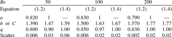
Figure 4 indicates that (1.2) approximates the DNS data very well in both the cases of fitted
 $a$
(solid lines) and
 $a=1$
(dashed lines), and similar results were obtained using (1.4). While the minimum scatter
 ${\rm\Delta}S_{T,\infty }$
was obtained using (1.2) with fitted
 $a$
, because there was an extra fitting parameter in this case, results obtained using (1.2) with either fitted
 $a$
or
 $a=1$
are indistinguishable with the naked eye in figure 4, and a similar level of approximation was obtained using (1.4), see table 3. When using (1.2), the fitted
 $q$
was close to unity and it was equal to unity when invoking (1.4), with the difference between these approximations being much less than the r.m.s. normalized turbulent flame speed
 $s_{t}^{\prime }$
. We also tried another fitting equation, i.e.
 $S_{T,\infty }=S_{L}+bS_{L}^{q}{U^{\prime }}^{1-q}$
, because such a type of expression can also be found in the literature, e.g. see Appendix B in the review paper by Lipatnikov & Chomiak (Reference Lipatnikov and Chomiak2002), and the DNS data were best fitted using
 $0<q\ll 1$
. Thus, the present DNS study supports the simplest linear combination of
 $S_{L}$
and
 $U^{\prime }$
, i.e. (1.4) with
 $q=1$
.
It is worth noting, first, that while the present DNS data support neither the theoretical (1.4) with
 $q=2$
nor the theoretical (1.4) with
 $q=4/3$
, this result should not be considered to disprove any of these theories (Clavin & Williams Reference Clavin and Williams1979; Aldredge & Williams Reference Aldredge and Williams1991; Kerstein & Ashurst Reference Kerstein and Ashurst1992, Reference Kerstein and Ashurst1994; Aldredge Reference Aldredge2006; Mayo & Kerstein Reference Mayo and Kerstein2007, Reference Mayo and Kerstein2008), because the theoretical constraint of
 $U^{\prime }\ll S_{L}$
was not reached in the present simulations. As discussed in detail elsewhere (Lipatnikov & Chomiak Reference Lipatnikov and Chomiak2002; Lipatnikov Reference Lipatnikov2012), the functional form of the dependence of the turbulent flame speed on the r.m.s. velocity can change with an increase in
 $U^{\prime }$
due to a change of the governing physical mechanisms. In particular, for this reason, we allowed
 $a\neq 1$
in (1.2) in the above discussion.
Second, the mean normalized speed
 $S_{T,\infty }/S_{L}$
, see figure 4, and the fitted values of the constant
 $b$
in (1.2) with
 $a=1$
or the constant
 $C$
in (1.4), see table 3, show a very weak increase with the Reynolds number, but the intervals
 $S_{T,\infty }/S_{L}\pm s_{t}^{\prime }$
computed for three different
 $\mathit{Re}$
overlap well, see figure 4. Therefore, the present DNS data should not be considered to show that the fully developed turbulent flame speed
 $S_{T,\infty }$
depends on the Reynolds number.
Third, because
 $S_{T,\infty }$
depends on the spatial correlation structure of the flow (Mayo & Kerstein Reference Mayo and Kerstein2008), the values of the parameters
 $a$
,
 $b$
and
 $C$
should not be considered to be universal. They can be sensitive to the forcing scheme similarly to other characteristics of turbulent flows evaluated in various DNS studies.
Fourth, figure 5 indicates that (1.2) with
 $q=2$
, which was highlighted by many researchers over six decades (Shchelkin Reference Shchelkin1947; Zimont & Pagnini Reference Zimont and Pagnini2011), is poorly supported by the present DNS data in the range of
 $0.5\leqslant U^{\prime }/S_{L}\leqslant 10$
. Although (1.2) with
 $q=2$
and
 $a=1$
approximates the DNS data obtained at
 $U^{\prime }/S_{L}\geqslant 5$
, cf. the dashed lines and symbols, it substantially underestimates the data computed at
 $U^{\prime }/S_{L}\leqslant 1$
, see figure 5(b). On the contrary, (1.2) with
 $q=2$
and fitted
 $a$
approximates the latter DNS data well, cf. the solid lines and symbols in figure 5(b), but overestimates the former ones, see figure 5(a). Nevertheless, it is worth noting that, at
 $U^{\prime }/S_{L}=10$
, the results yielded by (1.2) with
 $q=2$
and fitted
 $a$
are very close to the
 $S_{T,\infty }/S_{L}+s_{t}^{\prime }$
obtained by processing the DNS data at all three Reynolds numbers.
Fully developed normalized turbulent flame speed versus normalized r.m.s. velocity. Triangles, circles and squares show DNS data averaged over a long time interval of
 $5{\it\tau}_{t}^{0}<t<50{\it\tau}_{t}^{0}$
, associated with statistical stationarity of
 $S_{T}(t)=\text{d}\bar{{\it\xi}}^{S}/\text{d}t$
, with error bars indicating their normalized r.m.s. values, i.e.
 $\{\langle S_{T}^{2}(t)\rangle -\langle S_{T}(t)\rangle ^{2}\}^{1/2}/S_{L}$
, in the case of
 $\mathit{Re}=100$
. Solid and dashed lines approximate the DNS data using (1.2) with
 $q=2$
and fitted
 $a$
and
 $a=1$
respectively. The dot-dashed line was calculated using (1.3).

Fifth, figure 5(a) shows that the present DNS data definitely contradict (1.3), cf. the symbols with the dot-dashed line.
While the present and earlier (Wenzel & Peters Reference Wenzel and Peters2000) DNS data obtained by tracking an interface in a constant-density 3D turbulent flow support the linear dependence of the turbulent flame speed on both
 $S_{L}$
and
 $U^{\prime }$
, i.e. (1.2) with
 $q=1$
, it is worth noting certain effects that are well documented in the combustion literature but cannot be modelled within the framework of a paradigm of an infinitely thin front that self-propagates at a constant speed
 $S_{L}$
. First, bending of the
 $S_{T}(U^{\prime }/S_{L})$
curves, which is commonly associated with local flamelet quenching by turbulent stretching and/or finite thickness of flamelets, as reviewed elsewhere (Lipatnikov & Chomiak Reference Lipatnikov and Chomiak2002; Lipatnikov Reference Lipatnikov2012), is one example of such an effect. It was not simulated here, because the local burning rate was constant and the front thickness was infinitesimal. The bending effect was obtained in DNS by Wenzel & Peters (Reference Wenzel and Peters2000), who invoked a linear dependence of the front speed on its local curvature.
Second, an increase in turbulent flame speed by pressure (Lipatnikov & Chomiak Reference Lipatnikov and Chomiak2002; Lipatnikov Reference Lipatnikov2012) is another example. If (1.2) predicts an increase in
 $S_{T,\infty }$
by
 $S_{L}$
, then the same equation yields a decrease in
 $S_{T,\infty }$
with pressure
 $p$
if
 $S_{L}$
is decreased when
 $p$
is increased (the latter trend is typical for various hydrocarbon–air flames). On the contrary, certain models of turbulent combustion that allow for the thickness of the instantaneous flame front can predict the opposite effects of
 $p$
on
 $S_{T}$
and
 $S_{L}$
even if these models neglect the influence of combustion on the turbulence (Lipatnikov & Chomiak Reference Lipatnikov and Chomiak2002). However, the present authors are not aware of a model that neglects the front thickness, but is capable of predicting the opposite effects of
 $p$
on
 $S_{T}$
and
 $S_{L}$
. If pressure similarly affects both the fully developed
 $S_{T,\infty }$
shown in figure 4 and the developing
 $S_{T}$
addressed in a typical experiment, then the paradigm of infinitely thin fronts seems to miss some physical mechanisms that play an important role in premixed turbulent combustion. Nevertheless, even in such a case, the paradigm is worth studying, because it is an important building block for various models of turbulent burning, including models that allow for the front thickness. Moreover, a hypothesis that pressure similarly affects
 $S_{T,\infty }$
and
 $S_{T}$
requires proving, in spite of the fact that it is widely assumed.
Third, an increase in
 $S_{T,\infty }$
by the density ratio was obtained and associated with the Darrieus–Landau (DL) instability (Darrieus Reference Darrieus1938; Landau Reference Landau1944; Williams Reference Williams1985; Lipatnikov Reference Lipatnikov2012) in the previous DNS studies (Wenzel & Peters Reference Wenzel and Peters2000; Treurniet et al.
Reference Treurniet, Nieuwstadt and Boersma2006; Creta & Matalon Reference Creta and Matalon2011; Fogla et al.
Reference Fogla, Creta and Matalon2013) that dealt with the level set (2.3). A recent 3D-DNS study of weakly turbulent premixed flames in the case of a single reaction with a finite rate (Lipatnikov et al.
Reference Lipatnikov, Chomiak, Sabelnikov, Nishiki and Hasegawa2015) has clearly shown an important role played by the physical mechanism that causes the DL instability of laminar premixed flames.
4.2. Fully developed turbulent flame brush thickness
The normalized fully developed mean flame brush thickness
 ${\it\delta}_{T,\infty }/{\it\Lambda}$
, evaluated by averaging
 ${\it\delta}_{T}(t)=1/\!\max \!|\boldsymbol{{\rm\nabla}}\bar{c}|$
over a long time interval of
 $5{\it\tau}_{t}^{0}<t<50{\it\tau}_{t}^{0}$
, is shown by triangles, circles and squares in figure 6. Here,
 ${\it\delta}_{T}(t)$
and
 $\bar{c}(x,t)$
are associated with the long-living interface
 $G^{S}(\boldsymbol{x},t)=0$
, i.e.
 $\bar{c}(x,t)$
was evaluated by averaging
 $c^{S}(\boldsymbol{x},t)=H[G^{S}(\boldsymbol{x},t)]$
over
 $y$
and
 $z$
. Henceforth,
 $\max \bar{q}$
and
 $\min \bar{q}$
are calculated by varying
 $x$
for a mean quantity
 $\bar{q}(x)$
or
 $\bar{q}(x,t)$
.
Normalized fully developed mean flame brush thickness
 ${\it\delta}_{T,\infty }/{\it\Lambda}$
versus (a)
 $S_{L}/U^{\prime }$
and (b)
 $U^{\prime }/S_{L}$
. Triangles, circles and squares show DNS data averaged over a long time interval of
 $5{\it\tau}_{t}^{0}<t<50{\it\tau}_{t}^{0}$
, associated with statistical stationarity of
 ${\it\delta}_{T}(t)=1/\!\max \!|\boldsymbol{{\rm\nabla}}\bar{c}|$
. The curves fit the DNS data. Crosses show DNS data by Wenzel & Peters (Reference Wenzel and Peters2005).

The thickness does not depend on the Reynolds number and is decreased when
 $S_{L}$
is increased. The latter trend, revealed also by earlier DNS data (Wenzel & Peters Reference Wenzel and Peters2005), see the crosses, appears to be intuitively obvious, because the statistical stationarity of the thickness is reached due to a balance between an increase in
 ${\it\delta}_{T}$
by turbulent diffusion and a decrease in
 ${\it\delta}_{T}$
due to the self-propagation of the interface, whereas the thickness of a turbulent mixing layer, associated with vanishing
 $S_{L}$
, permanently grows with time and does not reach a statistically stationary limit. Minor quantitative differences between the present and earlier DNS data (Wenzel & Peters Reference Wenzel and Peters2005) on
 ${\it\delta}_{T,\infty }/{\it\Lambda}$
could be attributed to the use of different methods for evaluating
 ${\it\delta}_{T}(t)$
in the two studies.
Although a decrease in the fully developed mean flame brush thickness
 ${\it\delta}_{T,\infty }$
with an increase in
 $S_{L}$
is expected, many models do not allow for this effect and simply imply that or result in
 ${\it\delta}_{T,\infty }\propto {\it\Lambda}$
, e.g. see equation (2.156) in the book by Peters (Reference Peters2000). The present authors are aware of only three studies that predicted a decrease in
 ${\it\delta}_{T,\infty }$
with an increase in the laminar flame speed. First, Klimov (Reference Klimov1975) developed a model of premixed turbulent combustion by highlighting the consumption of large-scale flame-front wrinkles due to collisions of the front elements. The expressions reported by Klimov (Reference Klimov1975) yield
 ${\it\delta}_{T,\infty }\propto {\it\Lambda}(U^{\prime }/S_{L})^{q}$
with
 $q\approx 0.5$
. The dot-dashed lines in figure 6 show the best fit to the DNS data using a similar expression, i.e.
 ${\it\delta}_{T,\infty }/{\it\Lambda}=a(U^{\prime }/S_{L})^{1/2}$
. Comparison of these lines with the symbols indicates that the present DNS yield a weaker dependence of
 ${\it\delta}_{T,\infty }$
on
 $S_{L}$
. Indeed, when the power exponent
 $q$
in the scaling
 ${\it\delta}_{T,\infty }/{\it\Lambda}=a(U^{\prime }/S_{L})^{q}$
was varied, the DNS data were best fitted using
 $q\approx 1/3$
, see the solid lines.
Second, as pointed out by Sabelnikov (2014, private communication), an analysis by Kerstein & Ashurst (Reference Kerstein and Ashurst1992) results in
 ${\it\delta}_{T,\infty }/{\it\Lambda}\propto (U^{\prime }/S_{L})^{2/3}$
, i.e. a stronger dependence of the thickness on
 $U^{\prime }/S_{L}$
when compared with the present DNS study. This difference is not surprising, because Kerstein & Ashurst (Reference Kerstein and Ashurst1992) investigated the case of
 $U^{\prime }\ll S_{L}$
, whereas
 $U^{\prime }/S_{L}\geqslant 0.5$
in the present work.
Third, Zimont (Reference Zimont2000) has hypothesized that (i) a statistically stationary mean flame brush is reached when the rate
 $\text{d}{\it\delta}_{T}/\text{d}t$
of the growth of its thickness due to turbulent diffusion is equal to the laminar flame speed and (ii) the growth of the thickness during an earlier stage of the flame development is controlled by the turbulent diffusion law, i.e.
 ${\it\delta}_{T}\propto \sqrt{U^{\prime }{\it\Lambda}t}$
. These two hypotheses result straightforwardly in the scaling
 ${\it\delta}_{T,\infty }/{\it\Lambda}\propto U^{\prime }/S_{L}$
, but such a dependence of the thickness on the laminar flame speed is significantly stronger than the aforementioned result by Klimov (Reference Klimov1975) and is not supported by the present DNS data.
In the range of
 $U^{\prime }/S_{L}$
addressed in the present study, the solid lines
 ${\it\delta}_{T,\infty }/{\it\Lambda}\propto (U^{\prime }/S_{L})^{1/3}$
approximate the data well, but the widely accepted scaling of
 ${\it\delta}_{T,\infty }\propto {\it\Lambda}$
is not observed. The latter scaling was obtained by Wenzel & Peters (Reference Wenzel and Peters2005) by allowing for a linear dependence of the front propagation speed on its curvature. On the contrary, data reported in the same paper for the case of a constant
 $S_{L}$
fit the present data, cf. the crosses with the other symbols in figure 6.
It is also worth noting that an increase in
 ${\it\delta}_{T,\infty }$
by the density ratio was computed and associated with the DL instability in 2D DNS studies by Creta & Matalon (Reference Creta and Matalon2011) and Fogla et al. (Reference Fogla, Creta and Matalon2013) that dealt with the level set (2.3). A recent 3D-DNS study by Lipatnikov et al. (Reference Lipatnikov, Chomiak, Sabelnikov, Nishiki and Hasegawa2015) has also shown an increase in
 ${\it\delta}_{T,\infty }$
due to the physical mechanism that causes the DL instability of laminar premixed flames.
4.3. Self-propagating interface and turbulent scalar transport
Figure 7 shows the evolution of the normal (to the mean flame brush) profiles of the normal turbulent scalar flux
 $\overline{u^{\prime }c^{\prime }}(x,t)$
, see the broken lines. At any instant, the direction of the flux is consistent with the gradient diffusion paradigm, i.e.
 $\overline{u^{\prime }c^{\prime }}\leqslant 0$
and, therefore,
 $\overline{\boldsymbol{u}^{\prime }c^{\prime }}\boldsymbol{\cdot }\boldsymbol{{\rm\nabla}}\bar{c}\leqslant 0$
, with the peak value of
 $|\overline{u^{\prime }c^{\prime }}|$
being reduced with
 $t/{\it\tau}_{t}$
. The latter trend, associated with the growth of the mean flame brush thickness, as will be discussed later, is also shown in figure 8, where the minimum (over
 $x$
) negative values
 $\min \{\overline{u^{\prime }c^{\prime }}\}(t)/U^{\prime }$
of the normalized flux
 $\overline{u^{\prime }c^{\prime }}(x,t)/U^{\prime }$
are plotted versus the normalized flame-development time
 $t/{\it\tau}_{t}$
. It should be noted that the results reported at finite
 $t/{\it\tau}_{t}$
were computed by analysing transient interfaces
 $G_{m}^{T}$
during time intervals of
 $0<t^{\prime }/{\it\tau}_{t}^{0}\leqslant 2$
after the reset of
 $G_{m}^{T}(x_{m},t^{\prime }=0)=0$
, whereas the DNS data attributed to
 $t^{\prime }/{\it\tau}_{t}=\infty$
were obtained by analysing the long-living
 $G^{S}$
field at
 $5\leqslant t/{\it\tau}_{t}^{0}\leqslant 50$
.
Dependences of the normal scalar flux
 $\overline{u^{\prime }c^{\prime }}$
on the mean combustion progress variable, computed at various flame-development times specified in the legend and
 $\mathit{Re}=200$
, for (a)
 $S_{L}/U^{\prime }=0.1$
and (b)
 $S_{L}/U^{\prime }=1.0$
.

(a) Minimum (over
 $x$
) values
 $\min \{\overline{u^{\prime }c^{\prime }}\}(t)/U^{\prime }$
of the normalized flux
 $\overline{u^{\prime }c^{\prime }}(x,t)/U^{\prime }$
and (b) the integrated normalized flux
 $\int _{0}^{1}\overline{u^{\prime }c^{\prime }}\,\text{d}\bar{c}/U^{\prime }$
, computed at various normalized flame-development times
 $t/{\it\tau}_{t}$
in six DNS cases characterized by
 $S_{L}/U^{\prime }=0.1$
, 1.0 or 2.0 and
 $\mathit{Re}=50$
or 200.

Comparison of figures 8(a) and 8(b) indicates that the evolution of the integrated flux
 $\int _{0}^{1}\overline{u^{\prime }c^{\prime }}\,\text{d}\bar{c}$
closely follows the evolution of the flux magnitude
 $\min \{\overline{u^{\prime }c^{\prime }}\}$
, thus implying that the ratio of
 $\overline{u^{\prime }c^{\prime }}(x,t)/\min \{\overline{u^{\prime }c^{\prime }}\}(t)$
depends weakly on time, i.e.
 $$\begin{eqnarray}\overline{u^{\prime }c^{\prime }}(x,t)\approx \min \{\overline{u^{\prime }c^{\prime }}\}(t)f_{1}(x),\end{eqnarray}$$
where
 $f_{1}(x)$
is a function. This observation is further supported in figure 9, which shows results already plotted in figure 7, but renormalized using
 $\min \{\overline{u^{\prime }c^{\prime }}\}(t)$
.
Dependences of the renormalized scalar flux
 $\overline{u^{\prime }c^{\prime }}(x,t)/\min \{\overline{u^{\prime }c^{\prime }}\}(t)$
on the mean combustion progress variable, computed at various flame-development times specified in the legend and
 $\mathit{Re}=200$
, for (a)
 $S_{L}/U^{\prime }=0.1$
and (b)
 $S_{L}/U^{\prime }=1.0$
.

It should be noted that (4.2) is fully consistent with the gradient diffusion paradigm, which yields
 $f_{1}(x)=\boldsymbol{{\rm\nabla}}_{x}\bar{c}/\!\max \!|\boldsymbol{{\rm\nabla}}_{x}\bar{c}|$
, where
 $\boldsymbol{{\rm\nabla}}_{x}$
designates the partial derivative
 $\partial /\partial x$
along the direction
 $x$
, which is normal to the mean front. Such a relation roughly holds under the conditions of the present DNS study. Indeed, figure 10 indicates that the turbulent diffusivity
 $D_{t}=-\overline{u^{\prime }c^{\prime }}/\boldsymbol{{\rm\nabla}}_{x}\bar{c}$
normalized using
 $U^{\prime }{\it\Lambda}$
varies weakly within the mean flame brush, and the same trend was obtained in all other simulated cases. Accordingly, (4.2) can be reduced further to
 $$\begin{eqnarray}\overline{u^{\prime }c^{\prime }}(x,t)\approx {\it\delta}_{T}\min \{\overline{u^{\prime }c^{\prime }}\}(t)\boldsymbol{{\rm\nabla}}_{x}\bar{c}.\end{eqnarray}$$
Here,
 $\min \{\overline{u^{\prime }c^{\prime }}\}$
depends not only on the flame-development time, but also on the normalized interface speed
 $S_{L}/U^{\prime }$
, see figure 8(a), and
 ${\it\delta}_{T}(t)=1/\!\max \!|\boldsymbol{{\rm\nabla}}_{x}\bar{c}|$
is the mean flame brush thickness evaluated by applying the maximum gradient method to
 $\bar{c}(x,t)$
.
Dependences of the turbulent diffusivity
 $D_{t}=-\overline{u^{\prime }c^{\prime }}/\boldsymbol{{\rm\nabla}}_{x}\bar{c}$
normalized using
 $U^{\prime }{\it\Lambda}$
on the mean combustion progress variable, computed at various flame-development times specified in the legend and
 $\mathit{Re}=200$
, for (a)
 $S_{L}/U^{\prime }=0.1$
and (b)
 $S_{L}/U^{\prime }=1.0$
.

Using (4.3), we obtain
 $$\begin{eqnarray}D_{t}\equiv -\frac{\overline{u^{\prime }c^{\prime }}}{\boldsymbol{{\rm\nabla}}_{x}\bar{c}}=-{\it\delta}_{T}\!\min \{\overline{u^{\prime }c^{\prime }}\}(t),\end{eqnarray}$$
with (4.4) and figure 8(a) implying the development of
 $D_{t}$
. Indeed, figure 11(a) shows that the diffusivity averaged over the mean flame brush, i.e.
 $$\begin{eqnarray}D_{t}^{\ast }\equiv \int _{0}^{1}D_{t}\,\text{d}\bar{c}=-\int _{0}^{1}\frac{\overline{u^{\prime }c^{\prime }}}{\boldsymbol{{\rm\nabla}}_{x}\bar{c}}\,\text{d}\bar{c}=-\int _{0}^{L_{x}}\overline{u^{\prime }c^{\prime }}\,\text{d}x,\end{eqnarray}$$
grows as the flame develops, with (i) the DNS data being weakly sensitive to the Reynolds number under the conditions of the present study and (ii) almost the same
 $D_{t}^{\ast }$
being evaluated at
 $t/{\it\tau}_{t}<0.2$
in all cases. At larger
 $t/{\it\tau}_{t}$
, a higher
 $D_{t}^{\ast }$
and a longer development phase were obtained for a lower
 $S_{L}/U^{\prime }$
. It should be noted that figure 10 implies that
 $D_{t}(\bar{c})\approx D_{t}^{\ast }$
for any
 $\bar{c}$
.
Evolution of the flame-averaged diffusivity
 $D_{t}^{\ast }$
defined by (4.5): (a)
 $D_{t}^{\ast }/(U^{\prime }{\it\Lambda})$
versus
 $t/{\it\tau}_{t}$
and (b)
 $D_{t}^{\ast }/D_{t,\infty }^{\ast }$
versus
 $t/{\it\tau}^{\prime }$
, where
 ${\it\tau}^{\prime }=D_{t,\infty }^{\ast }/{U^{\prime }}^{2}$
. The solid line was calculated using (4.6) with
 ${\it\tau}_{L}={\it\tau}^{\prime }$
.

In the case of inert mixing, i.e.
 $S_{L}=0$
, the development of turbulent diffusivity is well known after the pioneering analysis by Taylor (Reference Taylor1935), which has resulted in particular in the following expressions:
 $$\begin{eqnarray}\displaystyle & \displaystyle D_{t}=D_{t,\infty }\left[1-\exp \left(-\frac{t}{{\it\tau}_{L}}\right)\right], & \displaystyle\end{eqnarray}$$
 $$\begin{eqnarray}\displaystyle & D_{t,\infty }=U^{\prime }{\it\Lambda}_{L}, & \displaystyle\end{eqnarray}$$
 ${\it\Lambda}_{L}$
and
 ${\it\tau}_{L}={\it\Lambda}_{L}/U^{\prime }$
are the Lagrangian length and time scales respectively. Figure 11(b) shows that (4.6), see the solid line, fits the present DNS data on
 $D_{t}^{\ast }$
well, see the symbols, provided that
 ${\it\tau}_{L}$
is substituted with
 ${\it\tau}^{\prime }=D_{t,\infty }^{\ast }/{U^{\prime }}^{2}$
. Accordingly, figures 10 and 11(b) imply that
 $$\begin{eqnarray}D_{t}=D_{t,\infty }^{\ast }\left[1-\exp \left(-\frac{{U^{\prime }}^{2}t}{D_{t,\infty }^{\ast }}\right)\right].\end{eqnarray}$$
Using (4.3), (4.4) and (4.8), we arrive at
 $$\begin{eqnarray}\overline{u^{\prime }c^{\prime }}(x,t)=-D_{t,\infty }^{\ast }\left[1-\exp \left(-\frac{{U^{\prime }}^{2}t}{D_{t,\infty }^{\ast }}\right)\right]\boldsymbol{{\rm\nabla}}_{x}\bar{c}\end{eqnarray}$$
and
 $$\begin{eqnarray}\min \{\overline{u^{\prime }c^{\prime }}\}=-\frac{D_{t,\infty }^{\ast }}{{\it\delta}_{T}}\left[1-\exp \left(-\frac{{U^{\prime }}^{2}t}{D_{t,\infty }^{\ast }}\right)\right].\end{eqnarray}$$
Figure 12(a) shows that the fully developed flame-averaged diffusivity
 $D_{t,\infty }^{\ast }$
is decreased when
 $S_{L}/U^{\prime }$
is increased, and the same trend is observed for
 $D_{t}(\bar{c})$
at any
 $\bar{c}$
, see figure 10. This trend appears to be mainly controlled by the decrease in the fully developed mean flame brush thickness with
 $S_{L}/U^{\prime }$
, as shown in figure 6. Indeed, the definition of
 $D_{t}$
given by (4.4) can be rewritten as follows:
 $$\begin{eqnarray}\frac{D_{t,\infty }^{\ast }}{U^{\prime }{\it\delta}_{T,\infty }}=-\frac{\overline{u^{\prime }c^{\prime }}}{U^{\prime }}\left(\frac{\partial \bar{c}}{\partial {\it\zeta}}\right)^{-1},\end{eqnarray}$$
where
 ${\it\zeta}=x/{\it\delta}_{T,\infty }$
is the distance normalized using the fully developed mean flame brush thickness. If we assume that the expression on the right-hand side of (4.11) does not depend on
 $S_{L}/U^{\prime }$
to the leading order, then the ratio of
 $D_{t,\infty }^{\ast }/(U^{\prime }{\it\delta}_{T,\infty })$
on the left-hand side should not depend on
 $S_{L}/U^{\prime }$
either. Indeed, figure 12(b) shows that the latter ratio, evaluated using the mean diffusivity
 $D_{t,\infty }^{\ast }$
, depends weakly on
 $S_{L}/U^{\prime }$
if
 $0.5\leqslant S_{L}/U^{\prime }\leqslant 2$
. The dependence of
 $D_{t,\infty }^{\ast }/(U^{\prime }{\it\delta}_{T,\infty })$
on the Reynolds number is not pronounced either. At low
 $S_{L}/U^{\prime }\leqslant 0.2$
, the ratio of
 $D_{t,\infty }^{\ast }/(U^{\prime }{\it\delta}_{T,\infty })$
decreases slightly on further decreasing
 $S_{L}/U^{\prime }$
.
(a) Flame-averaged fully developed normalized diffusivity
 $D_{t,\infty }^{\ast }/(U^{\prime }{\it\Lambda})$
and (b) the ratio of
 $D_{t,\infty }^{\ast }/(U^{\prime }{\it\delta}_{T,\infty })$
versus
 $S_{L}/U^{\prime }$
at various
 $\mathit{Re}$
specified in the legend.

Finally, (4.9) reads
 $$\begin{eqnarray}\overline{u^{\prime }c^{\prime }}(x,t)=-\frac{D_{t,\infty }^{\ast }}{{\it\delta}_{T,\infty }}\frac{{\it\delta}_{T,\infty }}{{\it\delta}_{T}}\left[1-\exp \left(-\frac{{U^{\prime }}^{2}t}{D_{t,\infty }^{\ast }}\right)\right]\frac{\partial \bar{c}}{\partial {\it\chi}},\end{eqnarray}$$
where
 ${\it\chi}=x/{\it\delta}_{T}$
is the distance normalized using the developing mean flame brush thickness
 ${\it\delta}_{T}(t)$
, i.e.
 $\max \!|\boldsymbol{{\rm\nabla}}_{{\it\chi}}\bar{c}|=1$
. Figure 13 validates (4.12) using all DNS data computed by us. Thus, (4.6) derived by Taylor (Reference Taylor1935) holds in the considered case provided that the Lagrangian length scale is substituted with
 $D_{t,\infty }^{\ast }/U^{\prime }=b_{1}{\it\delta}_{T,\infty }$
, where
 $b_{1}$
is slightly decreased when
 $S_{L}/U^{\prime }<0.5$
, but
 $b_{1}\approx 0.2$
is independent of
 $S_{L}/U^{\prime }$
if
 $0.5\leqslant S_{L}/U^{\prime }\leqslant 2$
, see figure 12(b).
Validation of (4.12) using all available DNS data.

It should be noted that (4.12) shows that the decrease in the magnitude of the flux
 $\overline{u^{\prime }c^{\prime }}$
with flame-development time, see figure 8, is controlled by the growth of the mean flame brush thickness
 ${\it\delta}_{T}(t)$
, whereas the development of the turbulent diffusivity, see the time-dependent term in square brackets, reduces the effect. As will be shown in the next subsection, the ratio of
 ${\it\delta}_{T,\infty }/{\it\delta}_{T}(t)$
is mainly controlled by
 $t/{\it\tau}^{\prime }={U^{\prime }}^{2}t/D_{t,\infty }^{\ast }\propto U^{\prime }t/({\it\delta}_{T,\infty })$
if
 $0.5\leqslant S_{L}/U^{\prime }\leqslant 2$
. Accordingly, (4.12) indicates that, under these conditions, the flux
 $\overline{u^{\prime }c^{\prime }}$
depends on the interface speed, mainly because the flux development is controlled by a time scale
 ${\it\delta}_{T,\infty }/U^{\prime }$
that depends on
 $S_{L}/U^{\prime }$
. Moreover, the flux depends straightforwardly on this ratio at a low
 $S_{L}/U^{\prime }$
, i.e. if
 $S_{L}/U^{\prime }$
is decreased, then the magnitude
 $|\overline{u^{\prime }c^{\prime }}|$
is decreased, because both
 $D_{t,\infty }^{\ast }/{\it\delta}_{T,\infty }$
and
 ${\it\delta}_{T,\infty }/{\it\delta}_{T}(t)$
are decreased, see figure 12 and figure 14(b) discussed in the next subsection. In other words, self-propagation of an interface in intense turbulence (
 $U^{\prime }\gg S_{L}$
) promotes the transport of a scalar that characterizes fluid before/behind the interface.
Normalized mean flame brush thickness (a)
 ${\it\delta}_{T}(t)/{\it\Lambda}$
versus
 $t/{\it\tau}_{t}$
and (b)
 $U^{\prime }{\it\delta}_{T}(t)/(2\sqrt{{\rm\pi}}D_{t,\infty }^{\ast })$
versus
 $t/{\it\tau}^{\prime }={U^{\prime }}^{2}t/D_{t,\infty }^{\ast }$
. The symbols show DNS data obtained at various
 $S_{L}/U$
specified in the legend. The blue, black and red symbols show data obtained at
 $\mathit{Re}=50$
, 100, and 200 respectively. The black solid lines show results computed using either (a) (4.13) at
 $\mathit{Re}=100$
(
 ${\it\tau}_{k{\it\varepsilon}}$
depends on
 $\mathit{Re}$
) or (b) (4.15). The red broken lines show results calculated using (4.17) and (4.18) at
 $S_{L}/U^{\prime }=0.1$
and 2.0.

For completeness, it is worth noting that turbulent scalar transport within a premixed turbulent flame brush is significantly affected not only by the propagation of the instantaneous flame front, but also by thermal expansion, with the latter effects being able to reverse the direction of the flux if
 $U^{\prime }/S_{L}$
is substantially less than the density ratio. This phenomenon, known as countergradient transport, is beyond the scope of the present work, but is discussed in detail elsewhere (Bray Reference Bray1995; Lipatnikov & Chomiak Reference Lipatnikov and Chomiak2010; Robin et al.
Reference Robin, Mura and Champion2011; Lipatnikov Reference Lipatnikov2012).
4.4. Development of mean flame brush thickness and turbulent flame speed
Figure 14(a) shows that the development of the normalized flame brush thickness persists for a long time interval, which is increased when
 $S_{L}/U^{\prime }$
is decreased and is longer than
 $2{\it\tau}_{t}$
if, e.g.,
 $S_{L}/U^{\prime }=0.1$
. Although this phenomenon is well known, it has not yet been incorporated into mainstream research into premixed turbulent combustion, and a model capable of predicting the development of
 ${\it\delta}_{T}(t)$
has not yet been elaborated.
A model developed by Peters (Reference Peters2000) yields
 $$\begin{eqnarray}{\it\delta}_{T}=b_{2}{\it\Lambda}\left[1-\exp \left(-\frac{c_{s}t}{{\it\tau}_{k{\it\varepsilon}}}\right)\right]^{1/2},\end{eqnarray}$$
where
 $b_{2}=1.78$
,
 $c_{s}=2.0$
and
 ${\it\tau}_{k{\it\varepsilon}}=\bar{k}/\bar{{\it\varepsilon}}\propto {\it\tau}_{t}$
. The black solid curve in figure 14(a) indicates that (4.13) with
 ${\it\tau}_{k{\it\varepsilon}}$
evaluated at
 $\mathit{Re}=200$
is contradicted by the DNS data, which clearly show that both
 ${\it\delta}_{T}$
and the time scale of its growth depend substantially on
 $S_{L}/U^{\prime }$
. Moreover, at
 $t\ll {\it\tau}_{t}$
, (4.13) yields
 ${\it\delta}_{T}\propto {\it\Lambda}\sqrt{t/{\it\tau}_{t}}$
, whereas the present DNS results plotted in figure 14(b) show a linear dependence of the mean flame brush thickness on time during the early stage of the flame development.
By reviewing experimental data obtained from various laboratory premixed turbulent flames, it was argued that the growth of the thickness is controlled by the turbulent diffusion law (Prudnikov Reference Prudnikov and Raushenbakh1967; Lipatnikov & Chomiak Reference Lipatnikov and Chomiak2002; Lipatnikov Reference Lipatnikov2012), i.e.
 ${\it\delta}_{T}(t)$
satisfies the following equation:
 $$\begin{eqnarray}\frac{\text{d}{\it\delta}_{T}^{2}}{\text{d}t}\propto D_{t}.\end{eqnarray}$$
By substituting (4.8) into the right-hand side of (4.14) we arrive at
 $$\begin{eqnarray}{\it\delta}_{T}^{2}=4{\rm\pi}D_{t,\infty }^{\ast }t\left\{1-\frac{D_{t,\infty }^{\ast }}{{U^{\prime }}^{2}t}\left[1-\exp \left(-\frac{{U^{\prime }}^{2}t}{D_{t,\infty }^{\ast }}\right)\right]\right\},\end{eqnarray}$$
where a factor of
 $4{\rm\pi}$
is used in order for the Gaussian distribution of
 $\boldsymbol{{\rm\nabla}}_{x}\bar{c}$
to be consistent with the definition of
 ${\it\delta}_{T}=1/\!\max \!|\boldsymbol{{\rm\nabla}}_{x}\bar{c}|$
(Lipatnikov & Chomiak Reference Lipatnikov and Chomiak2002).
At
 $t\ll {\it\tau}^{\prime }$
, (4.15) reads
 ${\it\delta}_{T}\propto U^{\prime }t$
, i.e. the thickness grows linearly with time and is independent of
 $S_{L}$
and
 $\mathit{Re}$
. Figure 14(b) validates (4.15) at
 $t/{\it\tau}^{\prime }\leqslant 2$
, including the linear scaling of
 ${\it\delta}_{T}\propto U^{\prime }t$
at
 $t\ll {\it\tau}^{\prime }$
. It is also worth noting that substitution of (4.15) into (4.12) followed by expansion of the obtained expression into a Taylor series at
 ${U^{\prime }}^{2}t/D_{t,\infty }^{\ast }\ll 1$
results in
 $$\begin{eqnarray}\min \{\overline{u^{\prime }c^{\prime }}\}=-\frac{U^{\prime }}{\sqrt{2{\rm\pi}}}\left[1-\frac{{U^{\prime }}^{2}t}{3D_{t,\infty }^{\ast }}\right],\end{eqnarray}$$
i.e. the magnitude of the flux decreases from
 $0.4U^{\prime }$
linearly with time, in line with figure 8(a). However, (4.15) is not applicable to the late stage of flame development.
Figure 14(b) indicates also that the normalized thickness
 $U^{\prime }{\it\delta}_{T}/(2\sqrt{{\rm\pi}}D_{t,\infty }^{\ast })$
depends neither on the Reynolds number nor on
 $S_{L}/U^{\prime }$
provided that
 $0.5\leqslant S_{L}/U^{\prime }\leqslant 2$
, but is increased when
 $S_{L}/U^{\prime }$
is further reduced, i.e.
 $S_{L}/U^{\prime }<0.5$
.
Scurlock & Grover (Reference Scurlock and Grover1953) argued that in order to apply the theory of turbulent diffusion by Taylor (Reference Taylor1935) to the development of mean flame brush thickness, the Lagrangian length
 ${\it\Lambda}_{L}$
and time
 ${\it\tau}_{L}$
scales should be substituted with the following scales:
 $$\begin{eqnarray}{\it\Lambda}_{f}=\frac{{\it\Lambda}_{L}}{1+S_{L}/(2U^{\prime })};\quad {\it\tau}_{f}=\frac{{\it\tau}_{L}}{1+S_{L}/(2U^{\prime })}=\frac{{\it\Lambda}_{f}}{U^{\prime }}\end{eqnarray}$$
and
 $$\begin{eqnarray}{\it\delta}_{T}^{2}=4{\rm\pi}{\it\Lambda}_{f}^{2}\frac{t}{{\it\tau}_{f}}\left\{1-\frac{{\it\tau}_{f}}{t}\left[1-\exp \left(-\frac{t}{{\it\tau}_{f}}\right)\right]\right\}.\end{eqnarray}$$
Comparison of the broken lines with the triangles and pluses in figure 14(a) shows that (4.17) and (4.18) predict (i) a decrease in the thickness when
 $S_{L}/U^{\prime }$
is increased and (ii) the development of
 ${\it\delta}_{T}$
at
 $S_{L}/U^{\prime }=0.1$
and
 $t\leqslant {\it\tau}_{t}$
, cf. the dashed line with the triangles. However, (4.17) and (4.18) underpredict or overpredict the influence of
 $S_{L}/U^{\prime }$
on the thickness at
 $t/{\it\tau}_{t}=O(1)$
or low
 $t/{\it\tau}_{t}$
respectively, cf. the dot-dashed line with the pluses.
Thus, although (4.15) describes the increase in the mean flame brush thickness during the early stage of premixed turbulent flame development well, we are not aware of a model that predicts
 ${\it\delta}_{T}(t)$
during the late stage of its growth.
Figure 15(a) shows that the development of the normalized turbulent flame speed persists also for a long time interval, which is increased when
 $S_{L}/U^{\prime }$
is decreased and is substantially longer than
 $2{\it\tau}_{t}$
if, e.g.,
 $S_{L}/U^{\prime }=0.1$
. Figure 15(b) indicates that, similarly to
 $U^{\prime }{\it\delta}_{T}/(2\sqrt{{\rm\pi}}D_{t,\infty }^{\ast })$
, the development of the normalized contribution
 $(S_{T}-S_{L})/(S_{T,\infty }-S_{L})$
of the turbulence to the flame speed as a function of the normalized time
 $t/{\it\tau}^{\prime }={U^{\prime }}^{2}t/D_{t,\infty }^{\ast }$
depends neither on the Reynolds number nor on
 $S_{L}/U^{\prime }$
provided that
 $0.5\leqslant S_{L}/U^{\prime }\leqslant 2$
, but is delayed when
 $S_{L}/U^{\prime }$
is further reduced, i.e.
 $S_{L}/U^{\prime }<0.5$
.
Normalized increase
 $(S_{T}-S_{L})/(S_{T,\infty }-S_{L})$
in flame speed
 $S_{T}(t)$
due to turbulence versus normalized flame-development time (a)
 $t/{\it\tau}_{t}$
or (b)
 $t/{\it\tau}^{\prime }={U^{\prime }}^{2}t/D_{t,\infty }^{\ast }$
. The various symbols show DNS data computed at various
 $S_{L}$
specified in the legend. The blue, black and red symbols show data obtained at
 $\mathit{Re}=50$
, 100 and 200 respectively.

The present authors are not aware of a model that yields an expression for growing
 $S_{T}(t)$
in the case of an infinitely thin flame front. However, in the case of a finite flame-front thickness, such an expression was derived (Lipatnikov & Chomiak Reference Lipatnikov and Chomiak1997, Reference Lipatnikov and Chomiak2002) by combining the Taylor theory and a model (Zimont Reference Zimont1979) of the burning velocity in intense (
 $S_{L}\ll U^{\prime }$
) Kolmogorov turbulence. Because the area of a material surface (
 $S_{L}=0$
) in Kolmogorov turbulence is mainly produced by small-scale eddies (Batchelor Reference Batchelor1952), the turbulent burning velocity was hypothesized (Lipatnikov & Chomiak Reference Lipatnikov and Chomiak1997, Reference Lipatnikov and Chomiak2002) to initially grow much faster when compared with the mean flame brush thickness, whose development is controlled by large-scale eddies characterized by a significantly larger time scale. Accordingly, the discussed model yields a larger
 $(S_{T}-S_{L})/(S_{T,\infty }-S_{L})\approx S_{T}/S_{T,\infty }$
when compared with
 ${\it\delta}_{T}/{\it\delta}_{T,\infty }$
. Subsequently, an ability to predict faster development of
 $S_{T}(t)$
when compared with
 ${\it\delta}_{T}(t)$
was proposed (Lipatnikov Reference Lipatnikov2009b
) to be a simple unified test for ranking various models of premixed turbulent combustion.
However, the present DNS data support neither this trend nor the aforementioned model. Figure 16 shows that
 $(S_{T}-S_{L})/(S_{T,\infty }-S_{L})$
grows faster than
 ${\it\delta}_{T}/{\it\delta}_{T,\infty }$
only if
 $S_{L}/U^{\prime }>1$
, but the difference is sufficiently small, cf. the open and filled diamonds or left-triangles and note that almost the same results were obtained at
 $\mathit{Re}=50$
and 200. At
 $S_{L}/U^{\prime }=1$
, the normalized flame speed and thickness develop similarly, cf. the open and filled squares, but
 ${\it\delta}_{T}/{\it\delta}_{T,\infty }$
grows substantially faster than
 $(S_{T}-S_{L})/(S_{T,\infty }-S_{L})$
if
 $S_{L}/U^{\prime }<1$
, with the difference being increased with a decrease in
 $S_{L}/U^{\prime }$
, e.g. cf. the open and filled up-triangles.
Development of
 $(S_{T}-S_{L})/(S_{T,\infty }-S_{L})$
, see the filled red symbols, and
 ${\it\delta}_{T}/{\it\delta}_{T,\infty }$
, see the open black symbols, computed at various
 $S_{L}$
specified in the legend and
 $\mathit{Re}=100$
.

4.5. Conditioned statistics of the turbulent flow field
The primary goal of this subsection is to investigate whether or not a conditioned moment of the velocity (or velocity gradient) field can be used to properly characterize the turbulence within a premixed flame brush. To answer this question, the true turbulence characteristics should be known and considered to be reference quantities for assessment of the conditioned ones. In the present study of constant-density and constant-viscosity flows, such reference turbulence characteristics are known, because self-propagation of an interface does not affect the flow. On the contrary, such reference turbulence characteristics have not yet been defined in a consistent manner in the case of combustion with heat release and density drop.
In the following, we will restrict ourselves to reporting results obtained in two representative cases, i.e.
 $\mathit{Re}=200$
and
 $S_{L}/U^{\prime }=0.1$
or 1.0, because the DNS data computed in other cases were qualitatively similar.
Figure 17 shows the evolution of the normal profiles of the normal velocity conditioned on unburned or burned mixture. In the case of two fluids separated by an infinitely thin interface, the moments of the
 $\boldsymbol{u}$
and
 $c$
fields can be evaluated by invoking the following bimodal joint probability density function (PDF) (Libby & Bray Reference Libby and Bray1981; Bray et al.
Reference Bray, Libby and Moss1985; Bray Reference Bray1995):
 $$\begin{eqnarray}P(\boldsymbol{u},c,x,t)=[1-\bar{c}(x,t)]{\it\delta}(c)P_{u}(\boldsymbol{u},x,t)+\bar{c}(x,t){\it\delta}(1-c)P_{b}(\boldsymbol{u},x,t),\end{eqnarray}$$
where
 $P_{u}(\boldsymbol{u},x,t)$
and
 $P_{b}(\boldsymbol{u},x,t)$
are velocity PDFs determined in unburned (
 $c=0$
) and burned (
 $c=1$
) fluids respectively, and
 ${\it\delta}(c)$
is the Dirac delta function. For brevity, the dependence of the PDFs and their moments on
 $x$
and
 $t$
will not be specified in the following expressions. Using (4.19) and the standard Bray–Moss–Libby (BML) technique (Libby & Bray Reference Libby and Bray1981; Bray et al.
Reference Bray, Libby and Moss1985; Bray Reference Bray1995), one can easily arrive at
 $$\begin{eqnarray}\bar{\boldsymbol{u}}=(1-\bar{c})\bar{\boldsymbol{u}}_{u}+\bar{c}\bar{\boldsymbol{u}}_{b}\end{eqnarray}$$
and
 $$\begin{eqnarray}\overline{\boldsymbol{u}^{\prime }c^{\prime }}=\bar{c}(1-\bar{c})(\bar{\boldsymbol{u}}_{b}-\bar{\boldsymbol{u}}_{u}).\end{eqnarray}$$
Because
 $\bar{u}=0$
in the coordinate framework used here, we have
 $$\begin{eqnarray}\overline{u^{\prime }c^{\prime }}=-(1-\bar{c})\bar{u}_{u}=\bar{c}\bar{u}_{b},\end{eqnarray}$$
i.e. the behaviour of the conditioned velocities is closely linked with the behaviour of the flux
 $\overline{u^{\prime }c^{\prime }}$
. In particular, (i) the magnitude of the slip velocity
 ${\rm\Delta}u=\bar{u}_{b}-\bar{u}_{u}$
is slightly increased by
 $S_{L}/U^{\prime }$
, in line with figures 7 and 8(a), and (ii) the magnitudes of the conditioned and slip velocities reduce as the flame develops.
Axial velocities normalized using
 $U^{\prime }$
and conditioned on unburned (
 $\bar{u}_{u}$
, top) or burned (
 $\bar{u}_{b}$
, bottom) mixture versus the mean combustion progress variable. The curves show DNS data obtained at various flame-development times specified in the legend and
 $\mathit{Re}=200$
, for (a)
 $S_{L}/U^{\prime }=0.1$
and (b)
 $S_{L}/U^{\prime }=1.0$
.

Figure 18 indicates that conditioned r.m.s. velocities should not be used to characterize the turbulence within a flame brush, because they differ substantially from the true r.m.s. turbulent velocity
 $\sqrt{\overline{{u^{\prime }}^{2}}}$
, which is well defined in the considered case. Indeed, within the framework of the BML approach (Libby & Bray Reference Libby and Bray1981; Bray et al.
Reference Bray, Libby and Moss1985; Bray Reference Bray1995), which holds under conditions of the present DNS, we have
 $$\begin{eqnarray}\overline{{u^{\prime }}^{2}}=\overline{u^{2}}=(1-\bar{c})(\overline{u^{2}})_{u}+\bar{c}(\overline{u^{2}})_{b}=(1-\bar{c})[\bar{u}_{u}^{2}+(\overline{{u^{\prime }}^{2}})_{u}]+\bar{c}[\bar{u}_{b}^{2}+(\overline{{u^{\prime }}^{2}})_{b}].\end{eqnarray}$$
This equation clearly shows that not only conditioned r.m.s. velocities
 $\sqrt{(\overline{{u^{\prime }}^{2}})_{u}}$
and
 $\sqrt{(\overline{{u^{\prime }}^{2}})_{b}}$
, but also conditioned velocities
 $\bar{u}_{u}$
and
 $\bar{u}_{b}$
contribute to the true r.m.s. turbulent velocity. Accordingly, we could expect that
 $(\overline{{u^{\prime }}^{2}})_{u}<\overline{{u^{\prime }}^{2}}$
and
 $(\overline{{u^{\prime }}^{2}})_{b}<\overline{{u^{\prime }}^{2}}$
, with the differences between the conventional and conditioned r.m.s. velocities being increased when
 $\bar{u}_{u}^{2}$
and
 $\bar{u}_{b}^{2}$
are increased. Indeed, in figure 18, these differences are most pronounced during an earlier stage of flame development, i.e. at a low ratio of
 $t/{\it\tau}_{t}$
, and the magnitudes of the conditioned velocities
 $\bar{u}_{u}$
and
 $\bar{u}_{b}$
are largest at low
 $t/{\it\tau}_{t}$
in figure 17. This significant difference should not be disregarded, because a large part of the volume of a typical laboratory flame is associated with
 $t/{\it\tau}_{t}<1$
.
Second moments normalized using
 ${U^{\prime }}^{2}=\overline{{u^{\prime }}^{2}}$
and conditioned on unburned (
 $(\overline{{u^{\prime }}^{2}})_{u}$
, top) or burned (
 $(\overline{{u^{\prime }}^{2}})_{b}$
, bottom) mixture versus the mean combustion progress variable. The curves show DNS data obtained at various flame-development times specified in the legend and
 $\mathit{Re}=200$
, for (a)
 $S_{L}/U^{\prime }=0.1$
and (b)
 $S_{L}/U^{\prime }=1.0$
.

Self-propagation of the interface increases the difference between the conventional and conditioned r.m.s. velocities evaluated at a late stage of flame development, i.e. the difference is increased by
 $S_{L}/U^{\prime }$
, cf. the solid curves in figures 18(a) and 18(b). However, the opposite trend can be observed at a low
 $t/{\it\tau}_{t}$
, e.g. cf.
 $(\overline{{u^{\prime }}^{2}})_{b}$
computed at
 $t/{\it\tau}_{t}=0.1$
and shown by dotted lines. It is worth also noting that
 $(\overline{{u^{\prime }}^{2}})_{b}$
is closer to
 $\overline{{u^{\prime }}^{2}}$
, whereas the difference in
 $\overline{{u^{\prime }}^{2}}$
and
 $(\overline{{u^{\prime }}^{2}})_{u}$
is larger.
Figure 19 shows that the conditioned third moments
 $(\overline{{u^{\prime }}^{3}})_{u}$
and
 $(\overline{{u^{\prime }}^{3}})_{b}$
are not proper turbulence characteristics, because they do not vanish in spite of the fact that the turbulence is isotropic and
 $\overline{{u^{\prime }}^{3}}=0$
in the present DNS, as verified in figure 7 in our previous paper (Yu et al.
Reference Yu, Lipatnikov and Bai2014). It is worth also noting that while the difference in
 $(\overline{{u^{\prime }}^{2}})_{u}$
or
 $(\overline{{u^{\prime }}^{2}})_{b}$
and
 $\overline{{u^{\prime }}^{2}}$
is reduced as the flame develops, see figure 18, the maximum (for various
 $\bar{c}$
) difference in
 $(\overline{{u^{\prime }}^{3}})_{u}$
or
 $(\overline{{u^{\prime }}^{3}})_{b}$
and
 $\overline{{u^{\prime }}^{3}}=0$
depends weakly on
 $t/{\it\tau}_{t}$
. For instance,
 $|(\overline{{u^{\prime }}^{3}})_{b}|$
evaluated at
 $\bar{c}=0.9$
and
 $t/{\it\tau}_{t}=0.1$
is approximately 0.2, but almost vanishes at large
 $t/{\it\tau}_{t}$
, whereas
 $|(\overline{{u^{\prime }}^{3}})_{b}|$
evaluated at
 $\bar{c}=0.1$
and
 $t/{\it\tau}_{t}=0.1$
almost vanishes, but is approximately 0.2 at large
 $t/{\it\tau}_{t}$
.
Third moments normalized using
 ${U^{\prime }}^{3}$
and conditioned on unburned (
 $(\overline{{u^{\prime }}^{3}})_{u}$
, top) or burned (
 $(\overline{{u^{\prime }}^{3}})_{b}$
, bottom) mixture versus the mean combustion progress variable. The curves show DNS data obtained at various flame-development times specified in the legend and
 $\mathit{Re}=200$
, for (a)
 $S_{L}/U^{\prime }=0.1$
and (b)
 $S_{L}/U^{\prime }=1.0$
.

As briefly summarized in § 1 and discussed in detail elsewhere (Lipatnikov Reference Lipatnikov2009a
; Lipatnikov & Chomiak Reference Lipatnikov and Chomiak2010; Lipatnikov Reference Lipatnikov2012), the basic difference between conditioned and canonical mean turbulence characteristics stems from the fact that conditional averaging is performed over a spatial domain whose boundary is wrinkled and randomly moves, with this motion being anisotropic. Moreover, due to the flux of a fluid through the boundary, e.g. conversion of reactants to products in flamelets, conditioned balance equations involve source or sink terms that do not appear in the counterpart Reynolds-averaged equations, e.g. see (4.25) and (4.26) below, with these source/sink terms substantially changing conditioned quantities when compared with the counterpart canonical Reynolds-averaged quantities. Because these source and sink terms are proportional to the front speed, variations in
 $S_{L}$
due to local curvature and straining of the front in the case of its finite thickness could also affect conditioned velocities. However, figure 17 indicates moderate sensitivity of
 $\bar{u}_{u}$
and
 $\bar{u}_{b}$
to variations in
 $S_{L}/U^{\prime }$
, thus implying that the aforementioned curvature and straining effects do not play a major role.
Recently, Yu et al. (Reference Yu, Lipatnikov and Bai2014) hypothesized that small-scale turbulence characteristics such as the total strain
 $S^{2}=0.25(S_{ij}+S_{ji})(S_{ij}+S_{ji})$
or enstrophy
 ${\it\omega}^{2}={\bf\omega}\boldsymbol{\cdot }{\bf\omega}=(\boldsymbol{{\rm\nabla}}\times \boldsymbol{u})\boldsymbol{\cdot }(\boldsymbol{{\rm\nabla}}\times \boldsymbol{u})$
are less sensitive to the method of taking an average (conventional or conditional) and, therefore, are better suited for characterizing turbulence within a flame brush. In the cited paper, this hypothesis was supported by DNS data averaged over a long time interval. Figure 20 further validates this hypothesis and shows that the differences between (i) conventional
 $\overline{S^{2}}$
and conditioned
 $(\overline{S^{2}})_{u}$
or
 $(\overline{S^{2}})_{b}$
and, especially, (ii) conventional
 $\overline{{\it\omega}^{2}}$
and conditioned
 $(\overline{{\it\omega}^{2}})_{u}$
or
 $(\overline{{\it\omega}^{2}})_{b}$
are sufficiently small at various stages of turbulent flame development, with
 $(\overline{{\it\omega}^{2}})_{b}$
being very close to
 $\overline{{\it\omega}^{2}}$
not only at various
 $t/{\it\tau}_{t}$
but also at various
 $\bar{c}>0.1$
, provided that
 $S_{L}/U^{\prime }=1.0$
, see figure 20(b).
Normalized conditioned enstrophy
 $(\overline{{\it\omega}^{2}})_{u}/\overline{{\it\omega}^{2}}$
or
 $(\overline{{\it\omega}^{2}})_{b}/\overline{{\it\omega}^{2}}$
(bottom) and normalized conditioned strain
 $(\overline{S^{2}})_{u}/\overline{S^{2}}$
or
 $(\overline{S^{2}})_{b}/\overline{S^{2}}$
(top) versus the mean combustion progress variable. The curves show DNS data obtained at various flame-development times specified in the legend and
 $\mathit{Re}=200$
, for (a)
 $S_{L}/U^{\prime }=0.1$
and (b)
 $S_{L}/U^{\prime }=1.0$
.

The suitability of the conditioned enstrophy for characterizing turbulence within a developing mean front is further evidenced in figure 21. While the difference between the true and conditioned r.m.s. turbulent velocities, see figure 21(a), is significant during the early stage of flame development, the difference between the conventional and conditioned enstrophies does not exceed 5 % in the middle of the flame brush (
 $\bar{c}=0.5$
) at various
 $\mathit{Re}$
and various
 $S_{L}/U^{\prime }$
, see figure 21(b).
Evolution of (a) the normalized conditioned r.m.s. velocity
 $(\overline{{u^{\prime }}^{2}})_{u}/\overline{{u^{\prime }}^{2}}$
or
 $(\overline{{u^{\prime }}^{2}})_{b}/\overline{{u^{\prime }}^{2}}$
and (b) the normalized conditioned enstrophy
 $(\overline{{\it\omega}^{2}})_{u}/\overline{{\it\omega}^{2}}$
or
 $(\overline{{\it\omega}^{2}})_{b}/\overline{{\it\omega}^{2}}$
, computed at
 $\bar{c}=0.5$
, for various
 $\mathit{Re}$
and
 $S_{L}/U^{\prime }$
specified in the legends.

It is worth remembering that, because a self-propagating interface does not affect the turbulent flow in the case of a constant density and a constant viscosity, the conventional moments of the velocity (or velocity gradient) fields are the true turbulence characteristics under the conditions of the present study. Accordingly, even if (i) the conditioned enstrophy is affected by density variations in the case of combustion with heat release and (ii) a study of such effects is beyond the scope of the present paper, the DNS data reported in figures 20 and 21 imply that variations in the conditioned enstrophy due to the heat release could consistently capture the influence of the heat release on the turbulence, whereas the conventional r.m.s. turbulent velocity is controlled not only by the turbulence, but also by the slip velocity induced due to the heat release, see (1.5).
Figure 22 shows that, contrary to the mean pressure gradient
 $\boldsymbol{{\rm\nabla}}\bar{p}$
, the conditioned pressure gradients
 $(\overline{\boldsymbol{{\rm\nabla}}p})_{u}$
and
 $(\overline{\boldsymbol{{\rm\nabla}}p})_{b}$
do not vanish within the mean front and have opposite signs, in line with the following BML equation (Bray et al.
Reference Bray, Libby and Moss1985):
 $$\begin{eqnarray}0=\boldsymbol{{\rm\nabla}}\bar{p}=(1-\bar{c})(\overline{\boldsymbol{{\rm\nabla}}p})_{u}+\bar{c}(\overline{\boldsymbol{{\rm\nabla}}p})_{b}.\end{eqnarray}$$
It should be noted that, contrary to combustion with heat release and density variations, associated with a finite pressure drop across an infinitely thin flame front, the pressure gradient conditioned to the interface vanishes in (4.24) in the case of a constant density. Figure 22 indicates also that the time dependence of the magnitude of
 $|(\overline{\boldsymbol{{\rm\nabla}}p})_{u}|$
or
 $|(\overline{\boldsymbol{{\rm\nabla}}p})_{b}|$
is non-monotonic and is more pronounced at
 $S_{L}/U^{\prime }=0.1$
when compared with
 $S_{L}/U^{\prime }=1$
.
The normal components
 $(\overline{\boldsymbol{{\rm\nabla}}_{x}p})_{u}$
and
 $(\overline{\boldsymbol{{\rm\nabla}}_{x}p})_{b}$
of the conditioned pressure gradients normalized using the fluid density and
 ${U^{\prime }}^{2}/{\it\Lambda}$
versus the mean combustion progress variable. The curves show DNS data obtained at various flame-development times specified in the legend and
 $\mathit{Re}=200$
, for (a)
 $S_{L}/U^{\prime }=0.1$
and (b)
 $S_{L}/U^{\prime }=1.0$
.

The fact that
 $(\overline{\boldsymbol{{\rm\nabla}}_{x}p})_{b}<0<(\overline{\boldsymbol{{\rm\nabla}}_{x}p})_{u}$
under the conditions of the present DNS implies that the conditioned pressure gradients reduce the magnitude of the slip velocity
 ${\rm\Delta}u=\bar{u}_{b}-\bar{u}_{u}$
. Indeed, in the case studied by us, the balance equations for the conditioned velocities
 $\bar{u}_{u}$
and
 $\bar{u}_{b}$
read (Im et al.
Reference Im, Huh, Nishiki and Hasegawa2004; Lipatnikov Reference Lipatnikov2008)
 $$\begin{eqnarray}\displaystyle & & \displaystyle \frac{\partial }{\partial t}[(1-\bar{c})\bar{u}_{u}]+\frac{\partial }{\partial x}[(1-\bar{c})\bar{u}_{u}^{2}]\nonumber\\ \displaystyle & & \displaystyle \quad =-\frac{\partial }{\partial x}[(1-\bar{c})(\overline{{u^{\prime }}^{2}})_{u}]-\frac{1-\bar{c}}{{\it\rho}}\overline{\left(\frac{\partial p}{\partial x}\right)}_{u}+(1-\bar{c}){\it\nu}\overline{\left(\frac{\partial ^{2}u}{\partial x_{k}^{2}}\right)}_{u}-S_{L}\bar{u}_{f}\overline{{\it\Sigma}}\end{eqnarray}$$
and
 $$\begin{eqnarray}\frac{\partial }{\partial t}(\bar{c}\bar{u}_{b})+\frac{\partial }{\partial x}(\bar{c}\bar{u}_{b}^{2})=-\frac{\partial }{\partial x}[\bar{c}(\overline{{u^{\prime }}^{2}})_{b}]-\frac{\bar{c}}{{\it\rho}}\overline{\left(\frac{\partial p}{\partial x}\right)}_{b}+\bar{c}{\it\nu}\overline{\left(\frac{\partial ^{2}u}{\partial x_{k}^{2}}\right)}_{b}+S_{L}\bar{u}_{f}\overline{{\it\Sigma}},\end{eqnarray}$$
where
 $\overline{{\it\Sigma}}$
is the mean interface surface density and
 $\bar{u}_{f}$
is the normal (to the mean front) velocity conditioned on the interface. Accordingly, the conditioned pressure gradient terms are negative and positive in unburned and burned mixtures respectively, thus reducing
 $\bar{u}_{u}$
, which is positive, see figure 17, increasing
 $\bar{u}_{b}$
, which is negative, and thus increasing
 ${\rm\Delta}u$
, which is also negative. On the contrary, the first terms on the right-hand sides of (4.25) and (4.26) are positive and negative respectively, see figure 18, thus controlling the negative signs of the terms
 ${\rm\Delta}u$
and
 $\overline{u^{\prime }c^{\prime }}$
under the conditions of the present DNS.
It is worth noting that the conditioned pressure gradients are relevant to modelling the following correlation
 $\overline{c^{\prime }\boldsymbol{{\rm\nabla}}p^{\prime }}$
, which plays a substantial role in the balance equation for the turbulent flux
 $\overline{u^{\prime }c^{\prime }}$
. Indeed, in the case of an infinitely thin interface, the joint PDF
 $P(p,c)$
can be modelled as follows:
 $$\begin{eqnarray}P(p,c)=(1-\bar{c}){\it\delta}(c)P_{u}(p)+\bar{c}{\it\delta}(1-c)P_{b}(p),\end{eqnarray}$$
within the framework of the BML approach. Therefore,
 $$\begin{eqnarray}\displaystyle \overline{c^{\prime }\boldsymbol{{\rm\nabla}}p^{\prime }} & = & \displaystyle -(1-\bar{c})\bar{c}[(\overline{\boldsymbol{{\rm\nabla}}p})_{u}-\boldsymbol{{\rm\nabla}}\bar{p}]+\bar{c}(1-\bar{c})[(\overline{\boldsymbol{{\rm\nabla}}p})_{b}-\boldsymbol{{\rm\nabla}}\bar{p}]\nonumber\\ \displaystyle & = & \displaystyle \bar{c}(1-\bar{c})[(\overline{\boldsymbol{{\rm\nabla}}p})_{b}-(\overline{\boldsymbol{{\rm\nabla}}p})_{u}].\end{eqnarray}$$
The following simple closure relation proposed first by Monin (Reference Monin1965):
 $$\begin{eqnarray}\overline{c^{\prime }\boldsymbol{{\rm\nabla}}p^{\prime }}=B_{2}\frac{\bar{{\it\varepsilon}}}{\bar{k}}\overline{\boldsymbol{u}^{\prime }c^{\prime }},\end{eqnarray}$$
where
 $B_{2}$
is a constant, is widely used in order to simulate inert turbulence mixing (Launder Reference Launder and Bradshaw1976). Accordingly, (4.21), (4.28), and (4.29) read
 $$\begin{eqnarray}(\overline{\boldsymbol{{\rm\nabla}}p})_{b}-(\overline{\boldsymbol{{\rm\nabla}}p})_{u}=B_{2}\frac{\bar{{\it\varepsilon}}}{\bar{k}}(\bar{\boldsymbol{u}}_{b}-\bar{\boldsymbol{u}}_{u}).\end{eqnarray}$$
Figure 23 supports (4.30) by showing that
 $B_{2}$
depends weakly on
 $\bar{c}$
and the flame-development time, with the exception of a very early (
 $t/{\it\tau}_{t}<0.2$
) stage of the flame development. However, figure 23 also indicates that
 $B_{2}$
is not a constant, but is increased when
 $S_{L}/U^{\prime }$
is decreased. Such a dependence of
 $B_{2}$
on
 $S_{L}/U^{\prime }$
is beyond the scope of a model of inert (
 $S_{L}=0$
) turbulent mixing, but can be of importance when modelling propagating fronts.
The parameter
 $B_{2}$
evaluated using (4.30) versus the mean combustion progress variable. The curves show DNS data obtained at various flame-development times specified in the legend and
 $\mathit{Re}=200$
, for (a)
 $S_{L}/U^{\prime }=0.1$
and (b)
 $S_{L}/U^{\prime }=1.0$
.

It is worth noting that the parameter
 $B_{2}$
averaged over the fully developed mean front, i.e.
 $B_{2,\infty }^{\ast }=\int _{0}^{1}\!B_{2,\infty }(\bar{c})\,\text{d}\bar{c}$
, correlates somehow with the normalized diffusivity
 $D_{t,\infty }^{\ast }/(U^{\prime }{\it\Lambda})$
averaged over the same front, see figure 24.
The flame-averaged fully developed constant
 $B_{2,\infty }^{\ast }=\int _{0}^{1}B_{2,\infty }(\bar{c})\,\text{d}\bar{c}$
versus the flame-averaged fully developed normalized diffusivity
 $D_{t,\infty }^{\ast }/(U^{\prime }{\it\Lambda})$
obtained in all DNS cases.

Finally, (4.25) and (4.26) involve the velocity
 $\bar{u}_{f}$
conditioned on the interface. Figure 25 shows that, at various flame-development times and
 $S_{L}/U^{\prime }$
, the behaviour of this velocity within the mean front is reasonably well fitted using the following simple linear interpolation (Lipatnikov Reference Lipatnikov2008):
 $$\begin{eqnarray}\bar{u}_{f}=\bar{c}\bar{u}_{u}+(1-\bar{c})\bar{u}_{b}\end{eqnarray}$$
between limit cases of
 $\bar{u}_{f}=(1-\bar{c})\bar{u}_{b}$
and
 $\bar{u}_{f}=\bar{c}\bar{u}_{u}$
, associated with the leading and trailing edges of the mean front respectively. It should be noted that
 $\bar{u}_{f}=\bar{u}_{b}$
or
 $\bar{u}_{f}=\bar{u}_{u}$
at the leading or trailing edge respectively, because the interface arrives at the leading (trailing) edge jointly with the burned (unburned) mixture.
Normal velocity
 $\bar{u}_{f}$
conditioned on the interface and normalized using
 $U^{\prime }$
versus the mean combustion progress variable. The symbols show DNS data obtained at various flame-development times specified in the legend and
 $\mathit{Re}=200$
, for (a)
 $S_{L}/U^{\prime }=0.1$
and (b)
 $S_{L}/U^{\prime }=1.0$
. The lines show results calculated using (4.31).

5. Conclusions
A 3D-DNS study of the evolution of a self-propagating interface in forced constant-density statistically stationary homogeneous isotropic turbulence was performed by solving Navier–Stokes and level-set equations under a wide range of conditions that cover various (from 0.1 to 2.0) ratios of the interface speed
 $S_{L}$
to the r.m.s. turbulent velocity
 $U^{\prime }$
and various (50, 100 and 200) turbulent Reynolds numbers
 $\mathit{Re}$
. The following results obtained by analysing DNS data are worth emphasizing.
-
(i) The computed fully developed normalized speed
 $S_{T,\infty }/U^{\prime }$
of the mean front depends almost linearly on
$S_{L}/U^{\prime }$
, thus supporting the classical linear relation between
$S_{T,\infty }$
,
$S_{L}$
and
$U^{\prime }$
under the conditions of the present study.
-
(ii) The fully developed normalized mean front thickness
${\it\delta}_{T,\infty }/{\it\Lambda}$
is reduced when the ratio of
$S_{L}/U^{\prime }$
is increased, with the DNS data being well fitted by the scaling
${\it\delta}_{T,\infty }/{\it\Lambda}\propto (S_{L}/U^{\prime })^{-1/3}$
. -
(iii) The fully developed mean turbulent flux
$(\overline{u^{\prime }c^{\prime }})_{\infty }$
of the scalar
$c$
that characterizes the state of the fluid (
$c=0$
and 1 ahead and behind the interface respectively) shows the gradient behaviour. The diffusivity associated with the flux and averaged over the fully developed flame brush, i.e.
$D_{T,\infty }^{\ast }=\int _{0}^{1}D_{T,\infty }(\bar{c})\,\text{d}\bar{c}$
, is decreased when the ratio of
$S_{L}/U^{\prime }$
is increased. The ratio of
$D_{T,\infty }^{\ast }/(U^{\prime }{\it\delta}_{T,\infty })$
is independent of
$0.5\leqslant S_{L}/U^{\prime }\leqslant 2.0$
, but is weakly decreased when
$S_{L}/U^{\prime }<0.5$
. -
(iv) During the development of the mean front, the evolution of the flux
$\overline{u^{\prime }c^{\prime }}$
is well described by (4.12), which results from the classical Taylor theory of turbulent diffusion, with the fully developed turbulent diffusivity
$D_{T,\infty }\propto U^{\prime }{\it\Lambda}$
being substituted with the fully developed front-averaged diffusivity
$D_{T,\infty }^{\ast }$
. -
(v) The development of the mean front speed and thickness requires a longer time when
$S_{L}/U^{\prime }$
is reduced. -
(vi) During the early stage of the mean front development, the growth of the mean front thickness is well described by the aforementioned Taylor theory provided that
$D_{T,\infty }$
is substituted with
$D_{T,\infty }^{\ast }$
. The growth of
${\it\delta}_{T}$
is linear with respect to the flame-development time
$t$
at least if
$t<D_{T,\infty }^{\ast }/{U^{\prime }}^{2}$
. -
(vii) Under the conditions of the present DNS study, there is no clear correlation between the growth of
${\it\delta}_{T}/{\it\delta}_{T,\infty }$
and
$(S_{T}-S_{L})/(S_{T,\infty }-S_{L})$
during the mean front development. The former ratio grows faster (slower) at a lower (higher)
$S_{L}/U^{\prime }$
. -
(viii) The conditioned moments of the velocity field differ substantially from the canonical Reynolds-averaged moments, whereas the conditioned and canonical mean enstrophies are close to one another. These results imply that, contrary to the conditioned moments of the velocity field, the conditioned enstrophy could be used for characterizing turbulence within a premixed flame brush.
-
(ix) The classical closure of the correlation
$\overline{c^{\prime }\boldsymbol{{\rm\nabla}}p^{\prime }}$
, which is given by (4.29) and is widely used in numerical simulations of turbulent mixing, holds under the conditions of the present DNS study provided that the closure parameter is increased by the diffusivity
$D_{T,\infty }^{\ast }$
. -
(x) Under the conditions of the present DNS study, the velocity conditioned on the interface is well approximated with the simplest linear equation (4.31).
-
(xi) All the aforementioned results are weakly sensitive to the turbulent Reynolds numbers addressed in the present study (
$50\leqslant \mathit{Re}\leqslant 200$
).














It is worth stressing that the simulations discussed in the present paper are the first computations in an ongoing DNS series aimed at improving our understanding of the governing physical mechanisms of premixed turbulent combustion by investigating a set of basic problems starting from the simplest one addressed in the present work. Subsequently, we plan (i) to complicate the problem step by step by allowing for a finite thickness of the flame front, then density variations and, finally, complex combustion chemistry and (ii) to reveal the role played by each of these effects by straightforwardly comparing data obtained in two subsequent sets of the DNS series. Accordingly, while the DNS data analysed in the present paper are relevant to premixed turbulent combustion, certain results can be substantially affected by the simplifications invoked. In particular, a finite thickness of the instantaneous flame front should be taken into account in order to predict the opposite effects of pressure on laminar and turbulent flame speeds, as discussed in § 4.1. Moreover, the influence of density variations on the flow field can play a substantial role in premixed turbulent combustion (Karlovitz, Denniston & Wells Reference Karlovitz, Denniston and Wells1951; Swaminathan & Grout Reference Swaminathan and Grout2006; Lieuwen Reference Lieuwen2012; Lipatnikov et al. Reference Lipatnikov, Chomiak, Sabelnikov, Nishiki and Hasegawa2015). For instance, the DL instability (Darrieus Reference Darrieus1938; Landau Reference Landau1944) was highlighted to be an important physical mechanism of weakly turbulent premixed combustion, e.g. see the review papers by Lipatnikov & Chomiak (Reference Lipatnikov and Chomiak2005, Reference Lipatnikov and Chomiak2010), as well as recent theoretical (Chaudhuri, Akkerman & Law Reference Chaudhuri, Akkerman and Law2011), numerical (Creta & Matalon Reference Creta and Matalon2011) and experimental (Troiani, Creta & Matalon Reference Troiani, Creta and Matalon2015) contributions.
Acknowledgements
R.Y. and X.S.B. gratefully acknowledge the financial support by the Swedish Research Council (VR) and the national Centre for Combustion Science and Technology (CeCOST). A.N.L. gratefully acknowledges the financial support by the Swedish Energy Agency and Chalmers Combustion Engine Research Center (CERC). The authors are very grateful to Professors J. Chomiak and V. Sabelnikov for fruitful discussion. The computation was performed using the computer facilities provided by the Centre for Scientific and Technical Computing at Lund University (LUNARC). We also acknowledge PRACE for awarding us access to resource supermuc based in Germany at Leibniz-Rechenzentrum in Garching near Munich.