1 Introduction
Laboratory and field measurements of vortical flows through and around arrays, of varying solid fraction
 $\unicode[STIX]{x1D719}$
, have highlighted many interesting and practical phenomena (Davidson et al.
Reference Davidson, Myline, Jones, Phillips, Perkins, Fung and Hunt1995; Taddei, Manes & Ganapathisubramani Reference Taddei, Manes and Ganapathisubramani2016), but more detailed studies over a wide range of Reynolds number are needed to quantify and explain the general results and the complex effects of these unsteady inhomogeneous flows on the upwind, internal and downwind velocity and force statistics. To further our understanding of this topic the specific questions we ask in this work are:
(i) How is the incident flow modified in front, sides and near wake of the array?
(ii) How do variations of solid fraction affect the velocity fluctuations inside the array and the forces on individual cylinders and on the array as a whole?
The motivation behind this work is that many industrial and environmental engineering studies involve modelling the flow past isolated groups of long slender obstacles which may be rigid or flexible; a few examples are the tidal flows past turbines (Martin-Short et al. Reference Martin-Short, Hill, Kramer, Avdis, Allison and Piggott2015), flow past riser groups under oil rigs (Constantinides, Oakley & Holmes Reference Constantinides, Oakley and Holmes2006), dispersion of organic waste due to caged farmed fish (Wu et al. Reference Wu, Chaffey, Law, Greenberg, Drozdowski, Page and Haigh2014), flow through vegetation in near-coastal regions (Nepf Reference Nepf1999) and the interaction of an incident flow (composed of a current and waves) with many structural members (Santo et al. Reference Santo, Taylor, Williamson and Choo2014). In these applications it is possible that the incident flow is unsteady due to a turbulent boundary layer or the presence of a larger upstream body. It is necessary to study the effect of an unsteady flow on these idealised arrays before progressing to more complex configurations.
The modelling first requires characterising the properties of the incident unsteady flow
 $U_{I}$
advected by a uniform stream
 $U_{\infty }$
in relation to the geometrical properties. Following Hunt & Savill (Reference Hunt and Savill2005) a measure of the unsteadiness and spatial scale of the inhomogeneity of the incident flow, we define the characteristic time (
 ${\mathcal{T}}$
) and length (
 ${\mathcal{L}}$
) scale as
 $$\begin{eqnarray}{\mathcal{T}}=\frac{U_{\infty }L_{I}}{u^{\prime }D_{G}},\quad {\mathcal{L}}=\frac{L_{I}}{D_{G}},\end{eqnarray}$$
where
 $T_{L}=L_{I}/u^{\prime }$
is the eddy turnover time with
 $u^{\prime }$
the root mean square (r.m.s.) streamwise velocity,
 $L_{I}$
is the integral scale (or eddy size) of the incident flow and
 $D_{G}$
is the array diameter. This type of definition needs to be adapted for different configurations. The upstream disturbance depends on the relative strength of the unsteadiness and flow inhomogeneity, with the comparison made against the characteristic advective time scale or a spatial scale relative to the size of the array. Four regimes can be broadly identified in terms of
 ${\mathcal{T}}$
and
 ${\mathcal{L}}$
being much greater or less than unity.
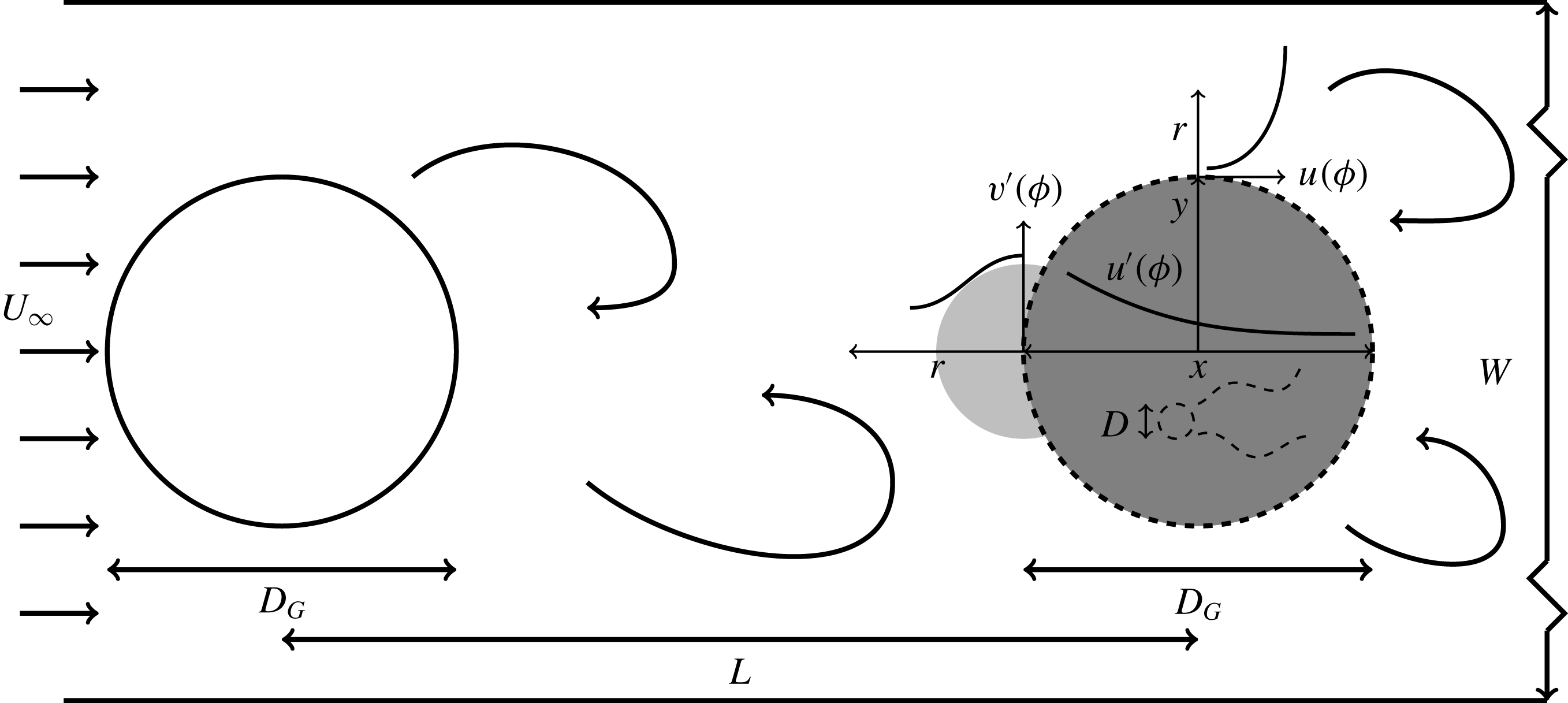
A schematic of the computational domain, of width
 $W=38D_{G}$
, is shown with an upstream cylinder and a downstream array (both of diameter
 $D_{G}$
) of varying solid fraction
 $\unicode[STIX]{x1D719}$
(dark grey) separated by a distance
 $L(=3.8D_{G})$
. The array is comprised of
 $N_{c}$
cylinders of diameter
 $D(=D_{G}/21)$
(see table 1 for properties of all the arrays considered in this study). The amplification of the tangential velocity in front of the array is shown in light grey (
 $O(D_{G})$
) where the theory of Hunt (Reference Hunt1973) is valid for high solid fraction arrays. Also highlighted are the decay of the fluctuations within the array and the width of the wake at the side of the array. The origin is located at the centre of the array. Figure not to scale.

For
 ${\mathcal{T}}\gg 1$
and
 ${\mathcal{L}}\gg 1$
, the incident flow is slowly varying or is quasi-steady with a weak spatial variation. Most research has been undertaken in this regime, which approximates to a uniform and steady incident flow. The low Reynolds number flow past a circular cylinder (in a steady incident flow) has been extensively studied in the early part of the last century. However it is only more recently that the effect of making the cylinder porous has been investigated. A general schematic for a porous region within a flow is shown in figure 1. Early work on uniform flow over disks (i.e. with no upstream cylinder as in figure 1) showed that their drag coefficient could be reduced by perforating the disk (Castro Reference Castro1971). However, by perforating a thin-walled cylinder the drag coefficient was greater than that of a solid cylinder (Alridge, Piper & Hunt Reference Alridge, Piper and Hunt1978). Nicolle & Eames (Reference Nicolle and Eames2011) used two-dimensional direct numerical simulations to investigate the steady flow past an array of stationary circular cylinders with a solid fraction varying from
 $0<\unicode[STIX]{x1D719}\leqslant 1$
. They identified three regimes (i) for
 $\unicode[STIX]{x1D719}<0.05$
the bodies do not interact with each other and so have a similar force response as an isolated cylinder; (ii) for
 $0.05<\unicode[STIX]{x1D719}<0.15$
the bleed from the group stabilises the fluctuating shear layers on either side of the array (for up to
 $5D_{G}$
downstream) resulting in a steady flow and a negligible lift coefficient and (iii) for
 $\unicode[STIX]{x1D719}>0.15$
the array starts to behave as a solid cylinder. The group drag coefficient was found to increase with increasing solid fraction and the maximum group drag coefficient was found to be at
 $\unicode[STIX]{x1D719}=0.3$
which was slightly greater (
 ${<}5\,\%$
) than the solid large cylinder (i.e.
 $\unicode[STIX]{x1D719}=1$
). Chang & Constantinescu (Reference Chang and Constantinescu2015) performed three-dimensional large eddy simulations, also with a steady incident flow, at
 $Re=10\,000$
(based on the group diameter) for
 $0.023<\unicode[STIX]{x1D719}<0.2$
and identified only two regimes, namely regimes (i) and (iii) from Nicolle & Eames (Reference Nicolle and Eames2011). Regime (ii) was not seen in the three-dimensional simulations as the shear layers became unstable and formed Kelvin–Helmholtz billows. Similar to the two-dimensional calculations, the group drag coefficient for
 $0.1\leqslant \unicode[STIX]{x1D719}\leqslant 0.2$
was greater than for
 $\unicode[STIX]{x1D719}=1$
. Arrays with the same solid fraction but with individual elements of a different diameter were found to have very different force coefficients. Two recirculation regions were observed downstream of the array (approximately
 $D_{G}$
) for
 $\unicode[STIX]{x1D719}=0.2$
.
The solid fraction
 $\unicode[STIX]{x1D719}=(D/D_{G})^{2}N_{c}$
of the arrays is varied by varying the number of cylinders (
 $N_{c}$
) in a region of constant area.

When
 ${\mathcal{L}}\gg 1$
but
 ${\mathcal{T}}$
is finite, we essentially have a body (or an array) within an incident unsteady flow. An example of this type of flow would be tidal currents in estuaries. Providing
 ${\mathcal{T}}\geqslant 5$
and the flow is not reversing, the broader characteristics can be understood from the steady incident flow problem and can be loosely described as quasi-steady. When
 ${\mathcal{T}}\leqslant 1$
, we tend to have a rapidly changing oscillatory flow which is similar to the passage of waves past large structures; at even higher values we have oscillatory boundary layers. While the problem of oscillatory flow past one body has been studied, the collective action of the flow around many bodies has not been widely studied. This lies outside the scope of this paper.
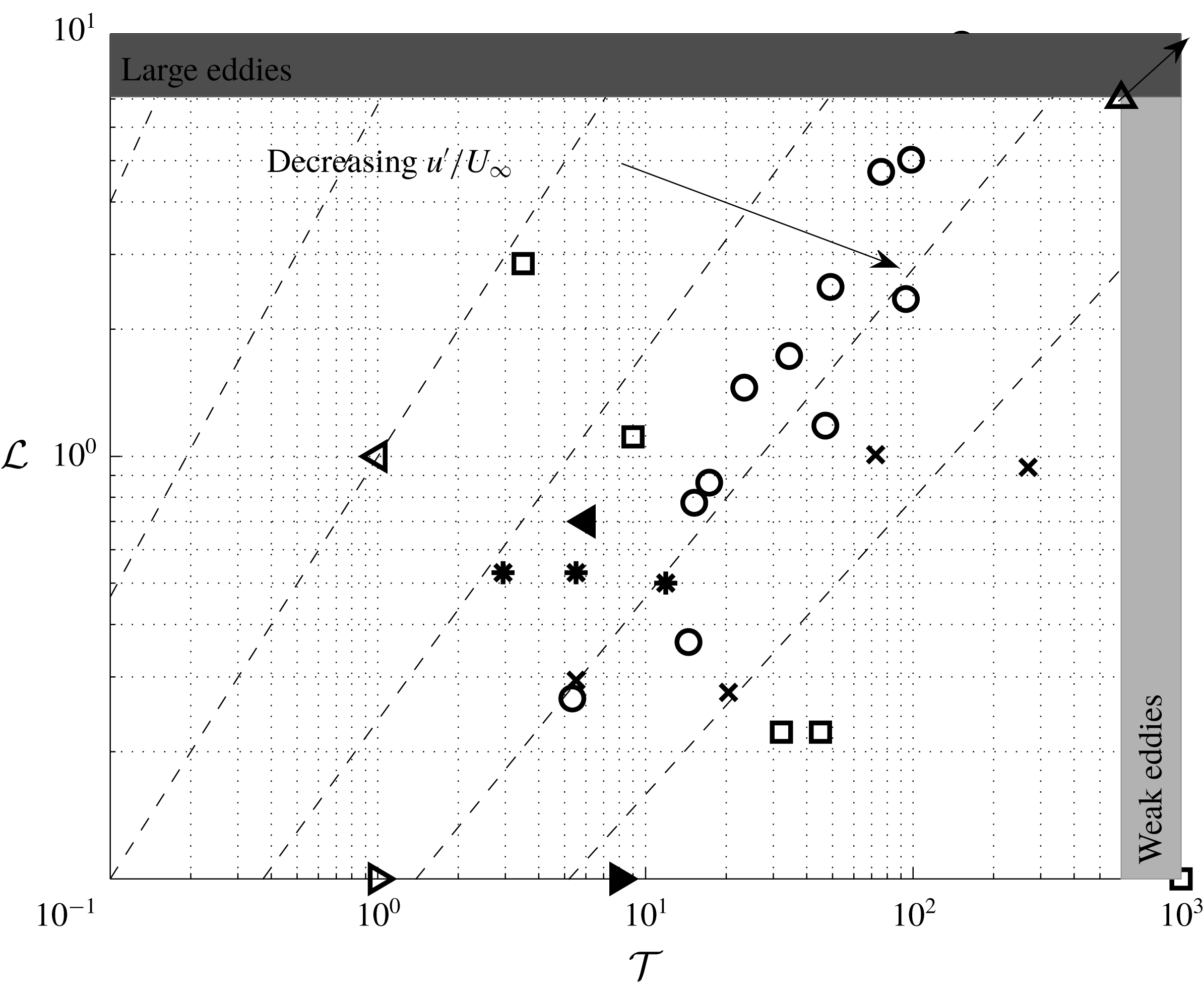
Approximate time and length scales for the different regions (highlighted in figure 1) in the current viscous simulations: uniform upstream
 $U_{\infty }$
(▵); large scale motion in between upstream cylinder and array (◃); wake behind a small cylinder for low solid fraction (▹) and for high solid fraction (▸); large scale motion shed by array for high solid fraction arrays (◂). Scatter plot showing research summary of different types of incident flow for flow past a single circular cylinder. Britter, Hunt & Mumford (Reference Britter, Hunt and Mumford1979) (experiments) (○); Norberg & Sunden (Reference Norberg and Sunden1987) (experiments) (
 $\times$
); Blackburn & Melbourne (Reference Blackburn and Melbourne1996) (experiments) (*); Surry (Reference Surry1972) (experiments) (▫); Nicolle & Eames (Reference Nicolle and Eames2011) (numerical) and Chang & Constantinescu (Reference Chang and Constantinescu2015) (numerical) (▵). The time and length scales are defined by (1.1).

When
 ${\mathcal{L}}\leqslant 1$
and
 ${\mathcal{T}}\gg 1$
, the upstream flow is inhomogeneous and unsteady and characterised by weak disturbances which are smaller than the size of the array. Figure 2 shows the experimental research on turbulent flow incident on a single cylinder. The focus of most of these studies was looking at how the turbulence affected the drag and lift force and the shedding frequency. Britter et al. (Reference Britter, Hunt and Mumford1979) investigated the effect of blocking on the velocity statistics in the vicinity of a single cylinder. Analytical methods used to analyse this interaction include rapid distortion theory (RDT) which refers to a mathematical technique that can be applied to analyse how weak turbulence (
 ${\mathcal{T}}\gg 1$
) is distorted due to the action of an ambient flow. This has provided understanding for the interaction of turbulence and boundaries, stratification, rotation and compression (see the reviews by Savill (Reference Savill1987) and Salhi & Cambon (Reference Salhi and Cambon2006)). For bluff body interactions Hunt (Reference Hunt1973), Graham (Reference Graham1976) and Durbin (Reference Durbin1981) applied it to understand the modification of a weak three-dimensional turbulent flow near the front of two- and three-dimensional rigid bodies and porous plates, respectively.
It is insightful to consider the various length and time scales in figure 1, which are also highlighted in figure 2. The incident flow on the upstream cylinder is uniform and steady and so
 ${\mathcal{L}}={\mathcal{T}}=\infty$
. For high
 $Re$
the upstream cylinder periodically sheds vorticity which results in velocity perturbations comparable to
 $U_{\infty }$
such that
 ${\mathcal{L}}={\mathcal{T}}=O(1)$
. The ability to shed vortices will be sensitive to the distance between the upstream cylinder and the array, which is further discussed in § 2. The effect of this flow on the downstream array will depend on the solid fraction of the array. For
 $\unicode[STIX]{x1D719}=1$
, the problem reduces to the case of large scale free stream unsteadiness impacting a boundary layer (see Hunt & Savill (Reference Hunt and Savill2005) for characteristics of this case). For individual cylinders in high solid fraction arrays, the large scale vortices cannot penetrate into the array. Also, there is no shedding from individual cylinders and vorticity annihilation occurs between shear layers of adjacent cylinders, resulting in weaker velocity fluctuations. For low solid fraction arrays the cylinders shed small scale vorticity into the flow where
 ${\mathcal{T}}\sim {\mathcal{L}}\ll 1$
. For the highest solid fraction arrays, there will be shedding from the array. However, due to the unsteady incident flow disrupting the shedding process, these vortices will be less intense and smaller than the ones from the upstream cylinder.
Based on the literature review, shown in figure 2, there is a clear research gap of unsteady incident flow past an array of cylinders and where
 $u^{\prime }/U_{\infty }\sim O(1)$
. However, it is this spatial and temporal non-homogeneity that makes this problem challenging but also representative of practical applications. In this study we consider the effect of an unsteady, inhomogeneous flow on an array of circular cylinders of varying solid fraction. In the limit of high solid fraction RDT simulations are carried out to investigate the effect of blocking on the velocity statistics of the incident flow in the vicinity of the array. In the limit of low solid fraction the interaction between the cylinders is weak and the force can be accurately estimated from the local slip velocity that occurs when the cylinders are removed.
We carry out high resolution two-dimensional numerical simulations at a moderate Reynolds number (
 $Re=2100$
) which limits the direct applicability of these simulations to industrial and environmental situations. However, there at this Reynolds number there is still sufficient complexity in the wake to be appropriate for this fundamental study. Additional RDT calculations are carried out as a means of extrapolating to a flow with a very high Reynolds number and the differences between these two approaches is explored. This comparison is possible as in three-dimensional RDT calculations past a two-dimensional body like a cylinder, the component
 $\unicode[STIX]{x1D714}_{3}$
is independent of
 $\unicode[STIX]{x1D714}_{1}$
and
 $\unicode[STIX]{x1D714}_{2}$
(Hunt Reference Hunt1973). Therefore this work provides a new approach for research and for industrial and environmental applications.
The paper is structured as follows; the problem is defined in § 2. In § 3 the mathematical models used for low and high solid fraction arrays are presented. The numerical methods used to carry out the direct numerical simulations and RDT calculations are described in § 4. The diagnostics which are applied to the numerical calculations are summarised in § 5. Plots of the vorticity field are discussed in § 6 to highlight the effect of solid fraction on the distortion of the vorticity field as it interacts with the array. The effect of the array on the velocity statistics adjacent and within the array are analysed in § 7. Inviscid RDT calculations are compared with the viscous simulations and differences are highlighted and discussed. The forces on individual cylinders and the array are presented and discussed in § 8. The results are discussed and conclusions are given in § 9.
2 Problem definition
Critical aspects of this work are the choices of the spatial array and unsteadiness of the incident flow. For arrays with a low solid fraction the overall shape of the array is less important than the individual body shapes within the array and their distribution. The array shape is critical at high solid fractions and having ‘sharp’ edges at square and rectangular arrays potentially generates behaviour that is not typical of many industrial problems. For this reason we chose a circular array with a structured placement of circular cylinders; this is the same array as Nicolle & Eames (Reference Nicolle and Eames2011) and gives a basis of comparison for the array of rigid cylinders in a steady incident flow. Similar configurations have been used in other multibody flow studies (Chang & Constantinescu Reference Chang and Constantinescu2015; Taddei et al. Reference Taddei, Manes and Ganapathisubramani2016).
Important choices are the types of unsteady incident flow to study and how to generate this flow. Previous work on unsteady flow incident on a rigid body has either focussed on homogeneous turbulent flow (Hunt Reference Hunt1973) or periodic gusts (Goldstein & Atassi Reference Goldstein and Atassi1976). In this paper the unsteady flow is chosen to be generated by an upwind cylinder (of equal array diameter
 $D_{G}$
) that is continuously shedding alternatively signed vortices. This flow is easily generated, gives reproducible results and provides a strong link to practical industrial and environmental problems as highlighted in the introduction. Additionally, in the limit that the array is a solid cylinder (i.e.
 $\unicode[STIX]{x1D719}=1$
), the problem reduces to that of two aligned cylinders which is an extremely well-studied case both numerically and experimentally (Zdravkovich Reference Zdravkovich1987), although the physics are still not completely understood (Lockard Reference Lockard2011).
The distance between the upstream cylinder and the array has been chosen to be large enough that the upstream cylinder can shed vortices which are advected downstream to interact with the array. If the upstream cylinder-array separation is below a critical value it can result in the shear layers from the upstream cylinder reattaching to the array (as was identified for the tandem cylinder case by Zdravkovich (Reference Zdravkovich1987)). This minimum distance is dependent on the vortex formation length (for the upstream cylinder in isolation) which is sensitive to the Reynolds number and additionally has a nonlinear dependence on the Reynolds number (see Norberg (Reference Norberg1987), figure 12). In two-dimensional numerical simulations reattachment ceases for a much smaller separation than for three-dimensional simulations (Papaioannou et al. Reference Papaioannou, Yue, Triantafyllou and Karniadakis2006).
As two-dimensional numerical simulations are performed it is worth discussing the effect of fully three-dimensional flow in this situation. For a given Reynolds number, vortices shed in two-dimensional simulations of flow past a cylinder are stronger and more coherent than those in three dimensions (Sumner Reference Sumner2010). Even though the wake behind a cylinder at higher Reynolds numbers is three-dimensional, it has been shown in Armstrong, Barnes & Grant (Reference Armstrong, Barnes and Grant1987) that the wake structure is still quite strongly two-dimensional with a von Kármán vortex street for
 $Re=21\,500$
. In three-dimensional flow, it is likely that instabilities will result in the partial or complete breakdown of these vortices as they impact the array, which will have a significant influence on the forces exerted on individual cylinders. Therefore quantitative agreement of velocity statistics in front of the array and forces (for two- and three-dimensional simulations) would not be expected however qualitative trends can be identified, similar to Nicolle & Eames (Reference Nicolle and Eames2011).
In this work a separation length of
 $L=3.8D_{G}$
was used and a group Reynolds number of 2100 (based on the upstream velocity
 $U_{\infty }$
and array diameter
 $D_{G}$
) was imposed. This leads to a Reynolds number of 100 based on the individual cylinder diameters. This was chosen so that (i) comparison could be made with Nicolle & Eames (Reference Nicolle and Eames2011), (ii) the minimum critical distance for shedding is achieved for that Reynolds number in two and three dimensions and (iii) this geometry is widely studied case for very high Reynolds numbers (Lockard Reference Lockard2011). A schematic of the problem is shown in figure 1.
3 Mathematical model
3.1 High solid fraction arrays
 $(\unicode[STIX]{x1D719}\geqslant 0.2)$

For high solid fraction arrays the primary interest is the modification of the flow caused by blocking induced by the collective action of the individual components of the array which is dominated by the upstream portion of the array.
3.1.1 Rapid distortion theory (RDT)
One method to analyse the influence of the array on the incident flow is to adapt the RDT model of Hunt (Reference Hunt1973) and Durbin (Reference Durbin1981). The RDT approach is a nonlinear calculation of how vorticity adjusts due to the differential advection of neighbouring fluid elements based on a linearisation of the perturbation caused by the inhomogeneous flow. Here, this is applied to examine the modification of an inhomogeneous flow past an array of cylinders. The velocity in the vicinity of the array can be expressed as
 $$\begin{eqnarray}\boldsymbol{u}=\bar{\boldsymbol{u}}_{0}+\boldsymbol{u}_{\unicode[STIX]{x1D714}},\end{eqnarray}$$
where
 $\bar{\boldsymbol{u}}_{0}$
is the steady mean flow around the array in the absence of the upstream wake and
 $\boldsymbol{u}_{\unicode[STIX]{x1D714}}$
is the unsteady flow generated by the incident wake on the array. The statistics and structure of
 $\boldsymbol{u}_{\unicode[STIX]{x1D714}}$
as
 $x\rightarrow -\infty$
are assumed to be known upstream of the array. While these are evolving in the streamwise direction, the change is relatively slow compared to the rapid change in the vicinity of the array. Since the ambient flow is irrotational it is useful to look at the evolution of the vorticity field. Writing
 $\unicode[STIX]{x1D714}_{\unicode[STIX]{x1D714}}=(\unicode[STIX]{x1D735}\times \boldsymbol{u}_{\unicode[STIX]{x1D714}})\boldsymbol{\cdot }\hat{\boldsymbol{z}}$
, the vorticity transport equation is
 $$\begin{eqnarray}\frac{\unicode[STIX]{x2202}\unicode[STIX]{x1D714}_{\unicode[STIX]{x1D714}}}{\unicode[STIX]{x2202}t}+(\bar{\boldsymbol{u}}_{0}+\boldsymbol{u}_{\unicode[STIX]{x1D714}})\boldsymbol{\cdot }\unicode[STIX]{x1D735}\unicode[STIX]{x1D714}_{\unicode[STIX]{x1D714}}=\unicode[STIX]{x1D708}\unicode[STIX]{x1D6FB}^{2}\unicode[STIX]{x1D714}_{\unicode[STIX]{x1D714}},\end{eqnarray}$$
since there is no vortex stretching in two dimensions (see Batchelor (Reference Batchelor1967), p. 268). Denoting the upstream velocity as
 $U_{\infty }$
and the length scale and root-mean-square velocity (of the streamwise component) of the incident flow by
 $L$
and
 $u^{\prime }$
, respectively, then the relevant parameters for the RDT approximation are
 $$\begin{eqnarray}Re_{\unicode[STIX]{x1D714}}=\frac{U_{\infty }^{2}L}{\unicode[STIX]{x1D708}}\gg 1,\end{eqnarray}$$
and
 $$\begin{eqnarray}\frac{u^{\prime }}{U_{\infty }}\ll 1.\end{eqnarray}$$
While the condition (3.3) is easily satisfied, the latter condition (3.4) in the numerical examples is only approximately satisfied. For random turbulent flow, the mean velocity induced by the vorticity field is zero, however for these structured and organised flows, the self-induced flow of the wake will have an impact on the mean flow upstream of the array.
3.1.2 Primary irrotational flow
Upstream of the array, the mean flow
 $\bar{\boldsymbol{u}}_{0}$
is irrotational. For a rigid cylinder (
 $\unicode[STIX]{x1D719}=1$
), the mean flow
 $\bar{\boldsymbol{u}}_{0}$
is to leading order irrotational except in a thin boundary layer on the upstream side and is characterised by strong shear layers at the sides. When
 $\unicode[STIX]{x1D719}=1$
, an approximate velocity field close to the array that satisfies the kinematic condition on the upwind face is
 $$\begin{eqnarray}\boldsymbol{u}_{0}=\unicode[STIX]{x1D735}\unicode[STIX]{x1D6F7}=U_{\infty }\left(1-\frac{(x^{2}-y^{2})D_{G}^{2}/4}{(x^{2}+y^{2})^{2}},\frac{-2xyD_{G}^{2}/4}{(x^{2}+y^{2})^{2}}\right).\end{eqnarray}$$
When
 $0<\unicode[STIX]{x1D719}<1$
, there are two options, the array can be treated as a porous cylinder or as a collection of physical cylinders. In this work only the latter case will be considered.
3.1.3 Velocity field calculation
When the constraints (3.3) and (3.4) are satisfied,
 $$\begin{eqnarray}\frac{\unicode[STIX]{x2202}\unicode[STIX]{x1D714}_{\unicode[STIX]{x1D714}}}{\unicode[STIX]{x2202}t}+\bar{\boldsymbol{u}}_{0}\boldsymbol{\cdot }\unicode[STIX]{x1D735}\unicode[STIX]{x1D714}_{\unicode[STIX]{x1D714}}=0,\quad \frac{\text{D}\unicode[STIX]{x1D714}_{\unicode[STIX]{x1D714}}}{\text{D}t}=0.\end{eqnarray}$$
The solution to the Lagrangian equation for vorticity is
 $$\begin{eqnarray}\unicode[STIX]{x1D714}_{\unicode[STIX]{x1D714}}(x,y,t)=\unicode[STIX]{x1D714}_{u}(x-U_{\infty }(\unicode[STIX]{x1D6E5}_{T}+t),y-\unicode[STIX]{x1D6E5}_{Y}),\end{eqnarray}$$
(Durbin Reference Durbin1981) where
 $\unicode[STIX]{x1D714}_{u}$
is the prescribed upstream wake vorticity,
 $\unicode[STIX]{x1D6E5}_{T}$
is the drift function,
 $\unicode[STIX]{x1D6E5}_{Y}$
is the vertical displacement function and
 $t$
is the time. A central feature of rapid distortion theory of flow past a body or array of bodies is the concept of drift (Hunt Reference Hunt1973). The drift of fluid particles is usually defined as
 $\unicode[STIX]{x1D6E5}_{T}$
which is the time taken for a particle starting at
 $(x_{0},y_{0})$
to get to
 $(X,Y)$
minus the time taken for the fluid particle to travel from
 $(x_{0},y_{0})$
to get to
 $(X,y_{0})$
without the body or bodies present such that
 $$\begin{eqnarray}\unicode[STIX]{x1D6E5}_{T}=\frac{1}{U_{\infty }}(X-U_{\infty }t-x_{0}).\end{eqnarray}$$
The vertical displacement of a fluid particle as it passes the array is
 $$\begin{eqnarray}\unicode[STIX]{x1D6E5}_{Y}=Y-y,\end{eqnarray}$$
and corresponds to the point above the initial cross-stream position far upstream. For
 $\unicode[STIX]{x1D719}=1$
the analytical form of
 $\unicode[STIX]{x1D6E5}_{T}$
and
 $\unicode[STIX]{x1D6E5}_{Y}$
is known (Hunt Reference Hunt1973).
3.1.4 Unsteady incident flow
Two-dimensional flow past an isolated cylinder at
 $Re=100$
exhibits the classic von Kármán vortex street wake. When the Reynolds number is increased to
 $Re=2100$
, the cylinder sheds vortices at oblique angles (see Nicolle & Eames (Reference Nicolle and Eames2011)). RDT requires as an input the wake generated by the upstream cylinder and one possibility of modelling this wake flow is by specifying the vorticity field as
 $$\begin{eqnarray}\displaystyle \unicode[STIX]{x1D714}_{w}(x_{0},y_{0}) & = & \displaystyle \mathop{\sum }_{j}\unicode[STIX]{x1D6FA}_{w}\left(\exp \left(-\frac{(x_{0}-(j-1/2N_{v})L_{v})^{2}+(y_{0}+A_{v}\sin \unicode[STIX]{x1D714}_{s}x_{0})^{2}}{R_{w}^{2}}\right)\right.,\nonumber\\ \displaystyle & & \displaystyle -\left.\exp \left(-\frac{(x_{0}-(j-1/2-1/2N_{v})L_{v})^{2}+(y_{0}+A_{v}\sin \unicode[STIX]{x1D714}_{s}x_{0})^{2}}{R_{w}^{2}}\right)\!\right)\!,\qquad\end{eqnarray}$$
where
 $\unicode[STIX]{x1D6FA}_{\unicode[STIX]{x1D714}}$
is the maximum vorticity,
 $R_{w}$
is the radius of the patch of vorticity,
 $N_{v}$
is the number of vortices and
 $L_{v}$
is the separation between the vortices. This is similar to the wake model used in Armstrong et al. (Reference Armstrong, Barnes and Grant1987). To capture the effect of the oblique shedding, a low frequency cross-stream displacement of the vortices is introduced,
 $A_{v}\sin \unicode[STIX]{x1D714}_{s}x_{0}$
, where
 $A_{v}$
and
 $\unicode[STIX]{x1D714}_{s}$
are the amplitude and frequency of this oscillation. Equation (3.10) does not capture the oblique motion explicitly, however it captures patches of vorticity propagating downstream at different cross-stream displacements. The choice of these parameters is determined by matching the velocity field statistics (i.e.
 $\bar{u}$
,
 $\bar{v}$
,
 $u^{\prime }$
and
 $v^{\prime }$
) of an isolated cylinder at
 $Re=2100$
(i.e. case
 $N_{0}$
) at an equivalent distance downstream (i.e. the array is situated at distance
 $3.8D_{G}$
downstream of the cylinder). The parameters which were used in this work were
 $A_{v}=D_{G}/2$
;
 $\unicode[STIX]{x1D714}_{s}=0.02$
;
 $\unicode[STIX]{x1D6FA}_{w}=1.2$
;
 $R_{w}=D_{G}/2$
;
 $N_{v}=500$
and
 $L_{v}=2.5D_{G}$
.
3.2 Low solid fraction arrays
$(\unicode[STIX]{x1D719}\ll 1)$

For low solid fractions and small cylinders (
 $D/D_{G}\ll 1$
), the whole array has a weak effect on the local upstream ambient flow and each element in the array tends to see the alternately signed vortical lumps propagating downstream. Using a similar method as Bagchi & Balachandar (Reference Bagchi and Balachandar2003) we try to estimate the force on the individual cylinders, by removing the cylinders and evaluating the contributions to the total force using the velocity and velocity gradients measured at the cylinder centre.
3.2.1 Flow and force characteristics of an array of isolated elements in an inhomogeneous flow
The force experienced by an isolated element (cylinder) may be estimated by adding together the inviscid and viscous flow contributions (Lighthill Reference Lighthill1986; Magnaudet & Eames Reference Magnaudet and Eames2000). This standard technique works because the inviscid contributions are largely determined by kinematic conditions and viscous effects are determined by the no-slip boundary condition. The force,
 $\boldsymbol{F}$
, is estimated to be a summation of various contributions
 $$\begin{eqnarray}\boldsymbol{F}(\boldsymbol{x},t)=\boldsymbol{F}_{D}+\boldsymbol{F}_{H}+\boldsymbol{F}_{I}+\boldsymbol{F}_{L},\end{eqnarray}$$
where
 $\boldsymbol{F}_{D}$
,
 $\boldsymbol{F}_{H}$
,
 $\boldsymbol{F}_{I}$
and
 $\boldsymbol{F}_{L}$
are the form drag, history, inertial, shear induced lift forces respectively. The drag force on a cylinder (diameter
 $D$
) is estimated as
 $$\begin{eqnarray}\boldsymbol{F}_{D}={\textstyle \frac{1}{2}}\unicode[STIX]{x1D70C}C_{D_{1}}D\boldsymbol{u}|\boldsymbol{u}|,\end{eqnarray}$$
where and
 $\boldsymbol{u}$
and
 $\unicode[STIX]{x1D70C}$
are the fluid velocity and density, respectively.
 $C_{D_{1}}(Re_{l})$
is an empirically determined coefficient, where
 $Re_{l}$
is the local Reynolds that the cylinder would experience if present (
 $Re_{l}=|\boldsymbol{u}|D/\unicode[STIX]{x1D708}$
), with the drag relationships
 $$\begin{eqnarray}\left.\begin{array}{@{}c@{}}C_{D}=9.689Re^{-0.78}(1+0.147Re_{l}^{0.82})\quad (0.1<Re_{l}<5),\\ C_{D}=9.689Re^{-0.78}(1+0.227Re_{l}^{0.55})\quad (5<Re_{l}<40),\\ C_{D}=9.689Re^{-0.78}(1+0.0838Re_{l}^{0.82})\quad (40<Re_{l}<400),\end{array}\right\}\end{eqnarray}$$
taken from Clift, Grace & Weber (Reference Clift, Grace and Weber1978). The history force is important when the local Reynolds number drops close to zero resulting in the surface vorticity diffusing into the ambient fluid and it not being advected away from the body resulting in changes to the force on the body. In this work the local Reynolds number
 $Re_{l}\gg 1$
and so this term will not be considered. The inviscid inertial force is estimated to be
 $$\begin{eqnarray}\boldsymbol{F}_{I}=\unicode[STIX]{x1D70C}(1+C_{m})\frac{\unicode[STIX]{x03C0}D^{2}}{4}\frac{\text{D}\boldsymbol{u}}{\text{D}t},\end{eqnarray}$$
where the added mass coefficient
 $C_{m}=1$
for a cylinder. This force can be interpreted as comprising a hydrostatic component (
 $-\unicode[STIX]{x1D735}p$
) and a contribution due to its shape (
 $-C_{m}A\unicode[STIX]{x1D735}p$
); the ratio of the former to the latter is
 $1:C_{m}$
. For two-dimensional flows the lift force that arises from an incident shearing flow is
 $$\begin{eqnarray}\boldsymbol{F}_{L}=C_{L}\unicode[STIX]{x1D70C}\boldsymbol{u}\times \unicode[STIX]{x1D74E}\boldsymbol{\cdot }\hat{\boldsymbol{z}},\end{eqnarray}$$
where
 $\unicode[STIX]{x1D74E}=\unicode[STIX]{x1D735}\times \boldsymbol{u}$
is the fluid vorticity. For inviscid flows, the lift coefficient
 $C_{L}=2$
(see Auton, Hunt & Prud’Homme Reference Auton, Hunt and Prud’Homme1988).
4 Numerical methods
Two types of two-dimensional numerical calculations were performed, namely viscous direct numerical and inviscid RDT simulations, which will be discussed in this section.
4.1 Direct numerical simulations
Figure 1 shows a schematic of the finite rectangular computational domain. The width
 $W=38D_{G}$
gives a blocking ratio of
 $W/D_{G}=0.026$
which ensures that the channel walls have a negligible effect (Kumar & Mittal Reference Kumar and Mittal2006). The upstream cylinder is a length
 $15.2D_{G}$
from the inlet and there is a centre–centre distance of
 $3.8D_{G}$
from the upstream cylinder to the array. The boundary conditions imposed on the computational domain are
 $U_{\infty }\hat{\boldsymbol{x}}$
on the inlet surface, kinematic and no-slip conditions on the rigid cylinders, zero flux on the side walls and a constant pressure constraint on the outlet.
The isothermal, incompressible Navier–Stokes equations were numerically solved using ACEsim which uses a characteristic-based-split scheme within a finite element framework; this code has been validated and successfully used for multi-body interactions (Nicolle & Eames Reference Nicolle and Eames2011). The defining equations are solved in three steps: involving first the calculation of an intermediate velocity field using the forcing by the viscous forces. The second step is the calculation of the pressure field, from the fact that the Laplacian of pressure is proportional to the divergence of the intermediate velocity. The pressure gradient is applied to force the intermediate velocity field to be solenoidal, and the updated velocity field is calculated in the third step.
The mesh specifications for the region adjacent to the upstream cylinder and downstream cylinder were chosen such that there was five elements across the boundary layer
 $\unicode[STIX]{x1D6FF}\sim dRe^{-1/2}$
(where
 $d=D_{G}(Re=2100)$
and
 $d=D(Re=100)$
for the upstream cylinder and for the individual cylinders respectively) which was estimated to be
 $\unicode[STIX]{x1D6FF}_{D_{G}}/D_{G}\sim 0.5$
and
 $\unicode[STIX]{x1D6FF}_{D}/D\sim 0.1$
, respectively. The mesh independence of these specifications was confirmed by performing an additional simulation of
 $N_{1}$
with double the resolution and the force statistics (coefficients and Strouhal numbers) on the single body agreed within 1 %.
4.2 Inviscid RDT simulations
The key step in applying RDT is to determine the relative travel times of fluid particles adjacent to one another on the same streamline or on adjacent streamlines. This relative motion gives rise to a significant compression and distortion local to the upstream stagnation point. The mathematical framework of Hunt (Reference Hunt1973) exploited and extended Darwin’s (Reference Darwin1953) work on fluid drift. Here we extend Hunt’s (Reference Hunt1973) model to two-dimensional wakes impacting on a circular array which in one limit is a cylinder.
RDT calculations require the calculation of the drift function
 $\unicode[STIX]{x1D6E5}_{T}$
and the
 $y$
-displacement function
 $\unicode[STIX]{x1D6E5}_{Y}$
. When we have an array with multiple cylinders present, an analytical solution is not readily available and therefore these variables need to be calculated numerically. The potential flow past the array is calculated numerically by solving
 $\unicode[STIX]{x1D6FB}^{2}\unicode[STIX]{x1D6F7}=0$
on a computational domain where the inlet and outlet are located
 $14.3D_{G}$
and
 $7.1D_{G}$
from the array centre respectively and has a width
 $38D_{G}$
. The boundary conditions imposed on the computational domain are
 $U_{\infty }\hat{\boldsymbol{x}}$
on the inlet surface and a no flux condition on the rigid cylinders and side walls. Fluid particles are released at the inlet (at regular intervals in the cross-stream) and the particles position is tracked by integrating forward in time. The distribution of
 $\unicode[STIX]{x1D6E5}_{T}$
and
 $\unicode[STIX]{x1D6E5}_{Y}$
on the finite element mesh can be obtained by interpolating the values of adjacent streamlines. The distorted wake vorticity can now be calculated from (3.7) and the velocity field is given by
 $$\begin{eqnarray}\boldsymbol{u}=\left(\frac{\unicode[STIX]{x2202}\unicode[STIX]{x1D6F9}}{\unicode[STIX]{x2202}y},-\frac{\unicode[STIX]{x2202}\unicode[STIX]{x1D6F9}}{\unicode[STIX]{x2202}x}\right),\end{eqnarray}$$
where the streamfunction satisfies
 $$\begin{eqnarray}\unicode[STIX]{x1D6FB}^{2}\unicode[STIX]{x1D6F9}=-\unicode[STIX]{x1D714}_{\unicode[STIX]{x1D714}}.\end{eqnarray}$$
The streamfunction is calculated using the finite element method within ACEsim. A unique solution to (4.2) is obtained by constraining the circulation around each cylinder to be zero, i.e.
 $$\begin{eqnarray}\unicode[STIX]{x1D6E4}_{i}=\oint _{S_{Bi}}\boldsymbol{u}\boldsymbol{\cdot }\text{d}\boldsymbol{S}=0,\end{eqnarray}$$
where
 $i=1,\ldots ,N_{c}$
. The solution requires the streamfunction value on each body to be specified which is not known a priori and must be determined through a search algorithm that exploits the linearity of (4.2).
5 Diagnostics
In this section we will present the key kinematic and dynamic diagnostics which are used in this work. The mean and root mean square of a time series
 $\unicode[STIX]{x1D709}(t)$
are defined as
 $$\begin{eqnarray}\frac{\bar{\unicode[STIX]{x1D709}}}{D}=\frac{1}{T_{2}-T_{1}}\int _{T_{1}}^{T_{2}}\unicode[STIX]{x1D709}\,\text{d}t,\quad \frac{\unicode[STIX]{x1D709}^{\prime }}{D}=\sqrt{\frac{1}{T_{2}-T_{1}}\int _{T_{1}}^{T_{2}}|\unicode[STIX]{x1D709}-\bar{\unicode[STIX]{x1D709}}|^{2}\,\text{d}t}.\end{eqnarray}$$
Time is non-dimensionalised as
 $\unicode[STIX]{x1D70F}=tU_{\infty }/D_{G}$
. The velocity statistics are non-dimensionalised as
 $u/U_{\infty }$
and
 $v/U_{\infty }$
. It should be noted that care is required when calculating the statistics because the time taken for the initial transient caused by starting the computations may be considerable (
 $\unicode[STIX]{x1D70F}\approx 60$
convective time units).
The force on a body is
 $$\begin{eqnarray}\boldsymbol{F}=\int _{S_{B}}(p\boldsymbol{I}-\unicode[STIX]{x1D749})\boldsymbol{\cdot }\hat{\boldsymbol{n}}\,\text{d}S,\end{eqnarray}$$
where
 $\hat{\boldsymbol{n}}$
is the normal vector pointing out of the fluid domain,
 $p$
is the fluid pressure,
 $\unicode[STIX]{x1D749}$
is the viscous stress tensor and the integration is taken over
 $S_{B}$
the surface of the body (see Batchelor (Reference Batchelor1967), p. 233). As the incident flow on the array is unsteady and inhomogeneous, in this work we will be using the force magnitude and angle instead of the traditional drag and lift coefficients. The total force coefficients on the individual cylinders (denoted as the
 $i$
th subscript) and the group force coefficient of
 $N_{c}$
cylinders are, respectively,
 $$\begin{eqnarray}C_{Ti}(t)=\frac{|\boldsymbol{F}_{i}|}{{\textstyle \frac{1}{2}}\unicode[STIX]{x1D70C}DU_{\infty }^{2}},\quad C_{TG}(t)=\frac{\displaystyle \mathop{\sum }_{i=1}^{N_{c}}|\boldsymbol{F}_{i}|}{{\textstyle \frac{1}{2}}\unicode[STIX]{x1D70C}D_{G}U_{\infty }^{2}},\end{eqnarray}$$
where
 $D$
is the cylinder diameter and
 $D_{G}$
is the diameter of the array. The instantaneous angle of the total force is defined as
 $$\begin{eqnarray}\unicode[STIX]{x1D703}_{|\boldsymbol{F}|i}(t)=\text{a tan}\left(\frac{\boldsymbol{F}_{i}\boldsymbol{\cdot }\hat{\boldsymbol{y}}}{\boldsymbol{F}_{i}\boldsymbol{\cdot }\hat{\boldsymbol{x}}}\right),\quad \unicode[STIX]{x1D703}_{|\boldsymbol{F}|G}(t)=\text{a tan}\left(\frac{C_{YG}}{C_{XG}}\right),\end{eqnarray}$$
for an individual cylinder or the array, respectively. The Strouhal number is the non-dimensional shedding frequency and is defined as
 $$\begin{eqnarray}St=\frac{fD_{G}}{U_{\infty }}.\end{eqnarray}$$
Snapshots of the vorticity field (ranging from
 $-1$
(blue) to 0 (green) to 1 (red)) at different times showing the effect of the downstream array (a–c)
 $N_{S1}$
and (d–f)
 $N_{133}$
on the patches of vorticity generated by the upstream cylinder (with the flow from left to right). For
 $N_{S1}$
, the patches of vorticity can be seen to slow down and distort around the cylinder which is due to streamwise biased tilting. For
 $N_{133}$
, the array is behaving similar to
 $N_{S1}$
but there is less intense shedding and secondary vorticity generation from the array. The Reynolds number is
 $Re=U_{\infty }D_{G}/\unicode[STIX]{x1D708}=2100$
.

Snapshots of the vorticity field (ranging from
 $-1$
(blue) to 0 (green) to 1 (red)) at different times showing the effect of the downstream array (a–c)
 $N_{95}$
and (d–f)
 $N_{64}$
on the patches of vorticity generated by the upstream cylinder. These two arrays are behaving similar to the other high solid fraction arrays shown in figure 3, with the large scale vortices not able to penetrate far into the array.

Snapshots of the vorticity field (ranging from
 $-1$
(blue) to 0 (green) to 1 (red)) at different times showing the effect of the downstream array (a–c)
 $N_{39}$
and (d–f)
 $N_{20}$
on the patches of vorticity generated by the upstream cylinder. For
 $N_{39}$
the individual cylinders shear layers are mainly attaching to downstream cylinders, however the cylinders on the periphery are shedding small scale vorticity into the flow. For
 $N_{20}$
, the separation between the cylinders is sufficient that they are mainly shedding vorticity into the flow. For both these cases the large vortices are capable of penetrating into the array.

Snapshots of the vorticity field (ranging from
 $-1$
(blue) to 0 (green) to 1 (red)) at different times showing the effect of the downstream array (a–c)
 $N_{7}$
and (d–f)
 $N_{1}$
on the patches of vorticity generated by the upstream cylinder. The large vortices move through the array at a near constant velocity and all the cylinders are shedding vorticity. Note the circular and elliptical shape of the vortices in (d–f) which is dependent on the sign of the small and large scale vorticity.

6 Qualitative description of flow processes
A starting point to understand the complex interaction between the unsteady flow generated by the upstream cylinder and the array is to discuss the features associated with the vorticity field; the kinematics and dynamics are discussed later. The incident flow on the upstream cylinder is uniform and characterised by a Reynolds number,
 $Re=2100$
. In two dimensions this results in the shedding of alternate signed vortices which are shed obliquely in a periodic fashion and are advected downstream (Nicolle & Eames Reference Nicolle and Eames2011). As can be seen in figures 3–6 reattachment of the shear layers of the upstream cylinder onto the array was not observed in any of the cases. The evolution of the vortices is then largely determined by the collective effect of the blocking and viscous drag of the individual cylinders in the array, which changes significantly with the array solid fraction. Since the flow is unsteady, the evolution of the vorticity field is shown with three representative snapshots that cover a span of time when a vortex shed from the upstream cylinder interacts with the array. The discussion will start with the case of
 $N_{S1}$
and will progress to arrays with lower
 $\unicode[STIX]{x1D719}$
.
The effect of a solid cylinder on the vortices is to slow them down and so the distance between consecutive vortices decreases (figure 3
a–c). As the vortex slows down it is also distorted by the favourable rate of strain of the mean streamwise velocity in front of the array (
 $|\unicode[STIX]{x2202}\bar{u}/\unicode[STIX]{x2202}y|>0$
), known as streamwise biased tilting. This feature, together with axial stretching, was identified to lead to the amplification of vorticity in front of a circular cylinder subject to an incident three-dimensional turbulent flow (Sadeh & Brauer Reference Sadeh and Brauer1980). The vortices interact with the array boundary layer and result in secondary vorticity being generated which is of the opposite sign to the incident vorticity. For
 $N_{133}$
and
 $N_{95}$
the arrays also shed large scale vorticity (figure 3
e,f), however the incident unsteady flow continually disrupts the formation of strong shear layers and so the subsequently shed vortices are smaller and with less circulation than the vortices shed from the upstream cylinder. For the high solid fraction arrays,
 $N_{64}$
and higher, the vortices do not penetrate far into the array and are forced around the array. Although the individual cylinders are generating shear layers of intense vorticity, the proximity of the cylinders means that these annihilate with shear layers of the opposite sign from adjacent cylinders (similar as in Nicolle & Eames (Reference Nicolle and Eames2011)) and so no vortices are shed from the individual members for the case of
 $N_{39}$
and above. Therefore the larger vortices moving around and downstream of the array do not have these smaller intense vortices present (figures 4
d–f and 5).
For the case of
 $N_{39}$
the proximity of the cylinders is such that the shear layers of the cylinders are mainly attaching to the downstream cylinders however the cylinders at the periphery are shedding into the larger vortices. For the case of
 $N_{20}$
and
 $N_{7}$
the individual cylinders are all shedding (whether they are interacting with a larger vortex or not). As the large vortices move through the array, the cylinders shed vorticity into the larger vortices (for the positive vortex in figure 6
b) which are then transported downstream. This can be seen to the bottom right of the array for the positive vortex in figure 6(c) where there are intense smaller vortices within the larger vortex. The blocking and viscous drag from the low solid fraction arrays is minimal and the vortices move towards, through and out of the array at an almost constant velocity, which can be seen by the constant distance between the negative (blue) and positive (yellow) vortices in figure 6(a–c). For the case
 $N_{1}$
the passage of a wake vortex changes the local slip velocity between the array elements leading to a von Kármán vortex street that is shed in a direction parallel to the local slip velocity. The local strain field induced by the large scale incident wake vortices causes the smaller opposite signed vortices to be circular, while vortices of the same sign (as the incident wake vortex) are elliptical (see figure 6
a,b).
Streamline plots of the mean velocity field through the array for the viscous simulations with an upstream cylinder; (a)
 $N_{S1}$
, (b)
 $N_{133}$
, (c)
 $N_{95}$
, (d)
 $N_{64}$
, (e)
 $N_{39}$
, (f)
 $N_{20}$
, (g)
 $N_{7}$
and (h)
 $N_{1}$
. The flow is from left to right and the streamline colour represents speed from low (blue) to high (red). The high solid fraction arrays have recirculation regions (a–c) and the black dashed-dot line in (b,c) show these penetrating into the array. Note the decelerated internal and near wake flow for the arrays
 $N_{64}$
to
 $N_{20}$
(d–f) and the cylinders behaving as isolated elements in (g,h).

Centreline streamwise velocity (a,c,e) and cross-stream profile of strain
 $\unicode[STIX]{x1D6F4}$
at
 $x/D_{G}=-3/4$
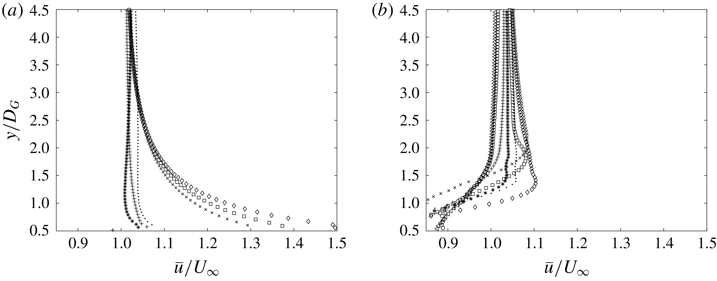
(b,d,f) for potential flow (a,b), viscous flow with a steady uniform incident flow (c,d) and viscous flow with an upstream cylinder present (e,f). The different solid fractions are represented by
 $N_{7}$
(○);
 $N_{20}$
(
 $+$
);
 $N_{39}$
(*);
 $N_{64}$
(
 $.$
);
 $N_{95}$
(
 $\times$
);
 $N_{133}$
(▫);
 $N_{S1}$
(♢). The lines in (a,b) are the analytical prediction for a porous region given by Eames & Bush (Reference Eames and Bush1999).

7 Kinematics
In this section the effect of the solid fraction on the blocking of an incident unsteady and inhomogeneous flow will be investigated. Rapid distortion theory will be used to gain insight into this process for the high solid fraction arrays. Three types of simulations will be considered: potential flow, steady incident flow viscous simulations (similar to Nicolle & Eames (Reference Nicolle and Eames2011)) and viscous simulations with an upstream cylinder. The discussion will be based around the upstream, side and internal flow and will be split into mean flow and second order statistics, always starting with the fully blocked case
 $N_{S1}$
and progressing to the lower solid fraction arrays.
7.1 Upstream of the array
7.1.1 Mean flow
To get an understanding of the average velocity field, streamline plots are presented in figure 7 where the streamlines are coloured by the magnitude of the mean velocity. This shows the deceleration of the streamwise velocity in front of the array and a divergence of the streamlines around the array for the high solid fraction arrays which decreases for lower solid fraction arrays. In figure 8(a) we compare potential flow simulations with the potential flow porous model given in Eames & Bush (Reference Eames and Bush1999). There is good agreement except that the porous model is not capable of capturing the velocity reduction close to the array,
 $O(D)$
, where the individual cylinders affect the flow field. The effect of including viscosity (while maintaining a steady incident flow) can be seen in figure 8(c). For
 $\unicode[STIX]{x1D719}=1$
, there is no effect upstream of the cylinder and so the streamwise velocity profiles are similar. However, for
 $\unicode[STIX]{x1D719}<1$
there is a significant difference in the streamwise velocity reduction. For example for
 $N_{133}$
,
 $\bar{u}/U_{\infty }|_{x/D_{G}=-1/2}\approx 0.75$
and 0.3 for the potential flow model and the steady incident viscous flow respectively (figure 8
a,c). The difference between these values is a result of the viscous drag present in the latter simulations and this effect decreases for lower solid fraction arrays. We can therefore distinguish between the upstream effects of inviscid kinematic blocking and viscous drag. In figure 8(e) we can see that if there is an unsteady incident flow there is a further reduction in the streamwise velocity component due to the upstream cylinder.
The mean strain field is insightful as it gives an indication to the distortion that can be expected to patches of vorticity in the vicinity of the array. Profiles of the strain at
 $x/D_{G}=-3/4$
are shown in figure 8(b,d,f). Similar results are obtained as for the streamwise velocity. The potential flow simulations give good agreement with the porous potential model except for the effect of the individual bodies for
 $\unicode[STIX]{x1D719}\ll 1$
(figure 8
b). Figure 8(d) shows the effect of including viscosity on the strain field. For
 $\unicode[STIX]{x1D719}=1$
the strain due to viscous drag is negligible and there is no modification to the upstream strain field. For
 $\unicode[STIX]{x1D719}<1$
the upstream strain field is modified significantly; for example the peak strain for the case of
 $N_{133}$
is an order of magnitude greater than the strain in the potential flow calculations (figure 8
b,d). For the current unsteady viscous simulations, the effect of the upstream wake is noticeable. For
 $\unicode[STIX]{x1D719}=1$
, the maximum strain is at
 $y/D_{G}=0$
which is similar to the potential flow and steady incident stream viscous simulations. For
 $\unicode[STIX]{x1D719}<1$
the strain field profiles are flatter and less than the case of a steady incident flow and the maximum strain occurs at
 $y/D_{G}\approx \pm 0.5$
(see figure 8
f).
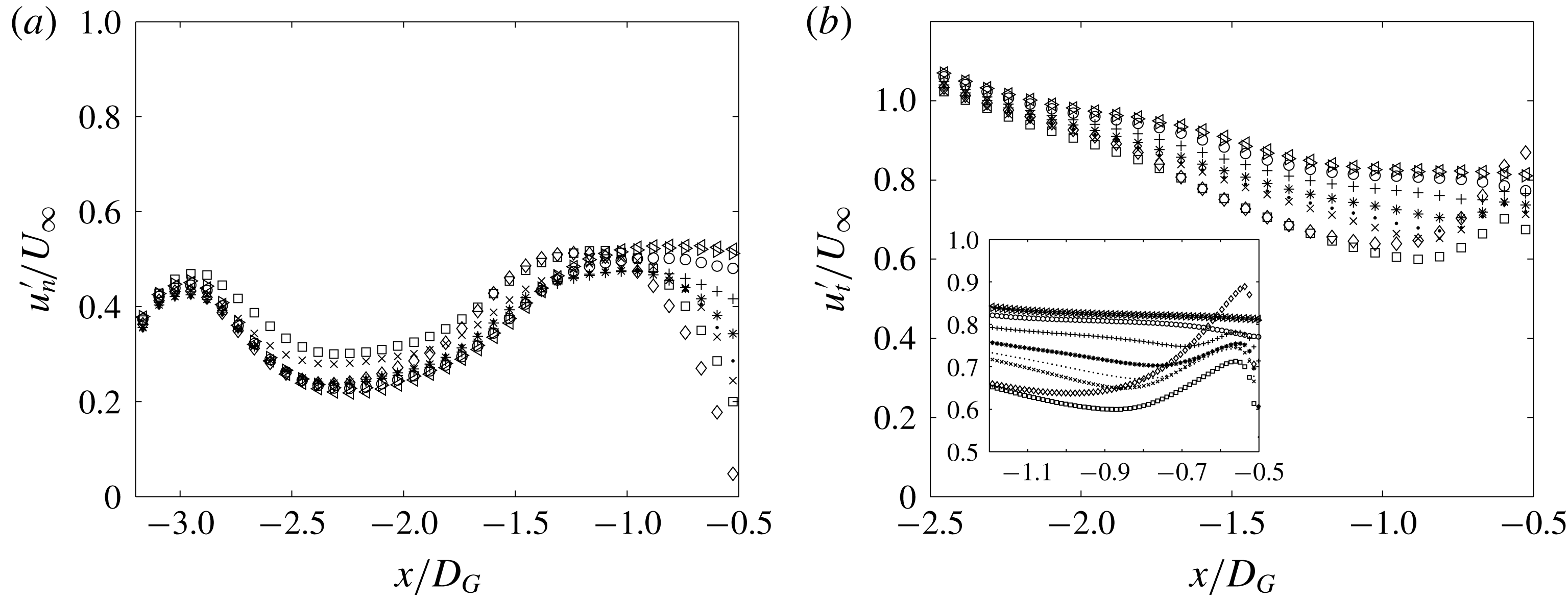
Streamwise profile of the root mean square (r.m.s.) of the (a) normal and (b) tangential velocity components for viscous simulations with an upstream cylinder, showing the reduction of the normal and the amplification of the tangential fluctuations respectively. The different solid fractions are represented by
 $N_{0}$
(
 ${<}$
);
 $N_{1}$
(
 ${>}$
);
 $N_{7}$
(○);
 $N_{20}$
(
 $+$
);
 $N_{39}$
(*);
 $N_{64}$
(
 $.$
);
 $N_{95}$
(
 $\times$
);
 $N_{133}$
(▫);
 $N_{S1}$
(♢). The centre of the upstream cylinder is located at
 $-3.8D_{G}$
.

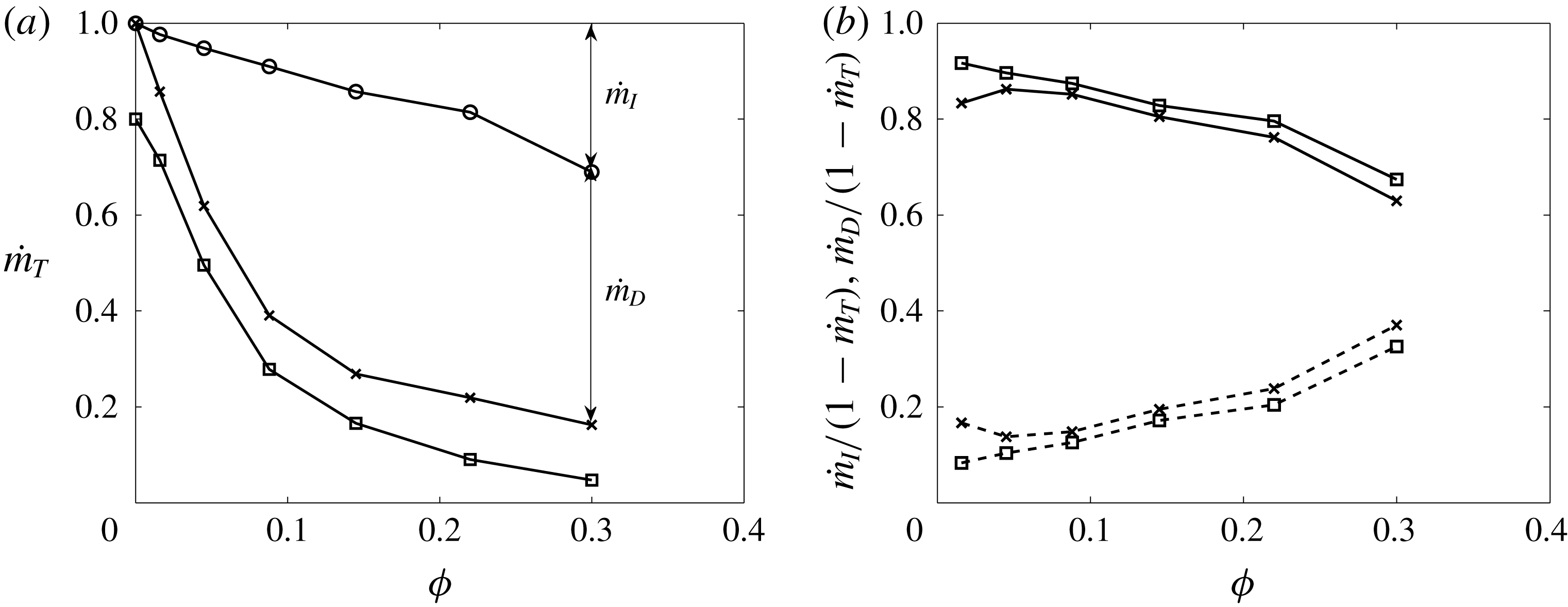
(a) The average mass flux
 ${\dot{m}}_{T}=\unicode[STIX]{x1D70C}\int _{-R}^{R}\bar{u}|_{x=0}\text{d}y/(U_{\infty }D_{G})$
through the array for potential flow (○) and for viscous numerical simulations for varying solid fraction. (b) Fraction of reduced mass flux through the array due to inviscid kinematic blocking
 ${\dot{m}}_{I}$
(dashed line) and viscous drag
 ${\dot{m}}_{D}$
(full line). In (a,b) the results shown are with (▫) and without (
 $\times$
) an upstream cylinder present.

7.1.2 Second order statistics
The r.m.s. of the streamwise and cross-stream components of the velocity are high near the upstream cylinder (centred at
 $x/D_{G}=-3.8$
) in figure 9 due to the vortex shedding process and these metrics decrease with distance downstream (towards the array). All of the arrays have a similar value of
 $u_{t}^{\prime }$
up to
 $x/D_{G}\approx -2$
, after which they start to deviate and, in general, the higher the solid fraction the more
 $u_{t}^{\prime }$
decreases. As successive lumps of alternate signed vorticity approach the cylinder they induce an image vorticity in the individual cylinders of the array (as a consequence of satisfying the kinematic boundary condition; see Hunt et al. (Reference Hunt, Kawai, Ramsey, Pedrizett and Perkins1990)). As the normal velocity component is reduced to zero (figure 9
a), this results in the amplification of the tangential component of the velocity. As there are alternate signed vortices being distorted above and below the array, this has no effect on the mean flow statistics. Blocking is greatest for
 $\unicode[STIX]{x1D719}=1$
and also the amplification occurs furthest from the array and the relative increase is highest. For
 $\unicode[STIX]{x1D719}<1$
, the greater
 $\unicode[STIX]{x1D719}$
, the greater the reduction in
 $u_{t}^{\prime }$
and although the relative amplification is higher in front of the array, the maximum tangential fluctuations in this region increases with decreasing
 $\unicode[STIX]{x1D719}$
(figure 9
b).
7.2 Around the sides of the array
7.2.1 Mean flow
Another way of analysing the effect of blocking and drag is by using an integral approach by calculating the average mass flux through the array (based on the mean velocity field). In figure 10(a) the potential flow calculations show a linear decrease in the mass flux through the array indicating a linear increase in inviscid blocking. The steady flow viscous numerical simulations show a significant decrease in the mass flux through the array which is due to the additional viscous drag. The effect of the unsteadiness of the current simulations does not have a significant effect on the mass flux through the array (see figure 10
a). In figure 10(b) it can be seen that for low
 $\unicode[STIX]{x1D719}$
the reduction of the mass flow through the array is due to viscous drag whereas as
 $\unicode[STIX]{x1D719}$
increases the reduction is increasingly due to inviscid blocking. A consequence of this is that there is an increased flow around the array for a higher solid fraction which would have important implications on scalar transport through and around the array.
When the upstream cylinder is absent (i.e. steady incident flow), figure 11(a) shows the sensitivity of the wake width with the solid fraction. For arrays
 $N_{39}$
and
 $N_{64}$
the shear layers at the sides of the array are stable for a far distance downstream, as was seen in Nicolle & Eames (Reference Nicolle and Eames2011). The consequence is that the flow within the array is essentially steady. For the solid fraction arrays
 $N_{95}$
and above these shear layers are unstable and the arrays behave like a solid body and shed large scale vorticity. For an upstream cylinder present, the flow near the array is dominated by the unsteady upstream wake and strong shear layers do not have the opportunity to form and so the wake width (at
 $x/D_{G}=0$
) is insensitive to the solid fraction (figure 11
b).
Cross-stream profile of the mean streamwise velocity at
 $x/D_{G}=0$
for (a) no upstream cylinder and (b) the upstream cylinder present, showing the weak dependence of the profile on solid fraction in (b). The different solid fractions are represented by
 $N_{0}$
(
 ${<}$
);
 $N_{1}$
(
 ${>}$
);
 $N_{7}$
(○);
 $N_{20}$
(
 $+$
);
 $N_{39}$
(*);
 $N_{64}$
(
 $.$
);
 $N_{95}$
(
 $\times$
);
 $N_{133}$
(▫);
 $N_{S1}$
(♢).

Contour plots of the root mean square of the (a) normal and (b) tangential velocity components in the near vicinity of the array for viscous simulations with an upstream cylinder present, showing the radial dependence of the velocity fluctuations. Contour plots of the arrays
 $N_{20}$
to
 $N_{S1}$
are stacked on top of each other with the array
 $N_{S1}$
at the bottom (
 $N_{c}$
is given at the right of the figure). The contour colours are from zero (blue) to one (red).
 $s$
is measured from the front stagnation point in the clockwise direction.

7.2.2 Second order statistics
When discussing the second order statistics around the side of the array it is more insightful to consider the velocity field in terms of tangential and normal components (relative to the array boundary). Figure 12(a) shows that for
 $\unicode[STIX]{x1D719}=1$
the normal fluctuations have to decrease to zero at the cylinder surface. For
 $\unicode[STIX]{x1D719}<1$
this condition is relaxed. In figure 12(b) it is possible to identify the increased fluctuations at
 $O(D)$
in the tangential velocity field due to the local distribution of the cylinders. Figure 12(b) shows that the r.m.s. of the tangential velocity at the front of the cylinder (
 $\unicode[STIX]{x1D719}=1$
) is approximately twice that at the sides (i.e.
 $u_{t}^{\prime }|_{\unicode[STIX]{x1D703}=\unicode[STIX]{x03C0}}\approx 2u_{t}^{\prime }|_{\unicode[STIX]{x1D703}=\unicode[STIX]{x03C0}/2}$
). To gain further insight into this, the velocity and vorticity are recorded at the points
 $\boldsymbol{x}_{1}/D_{G}=\{-0.57,0\}$
and
 $\boldsymbol{x}_{2}/D_{G}=\{0,0.57\}$
. At
 $\boldsymbol{x}_{1}$
there is both positive and negative vorticity peaks which results in a constant oscillation of the tangential velocity field. The processes at
 $\boldsymbol{x}_{2}$
are more complex. For the viscous simulations at the point
 $\boldsymbol{x}_{2}$
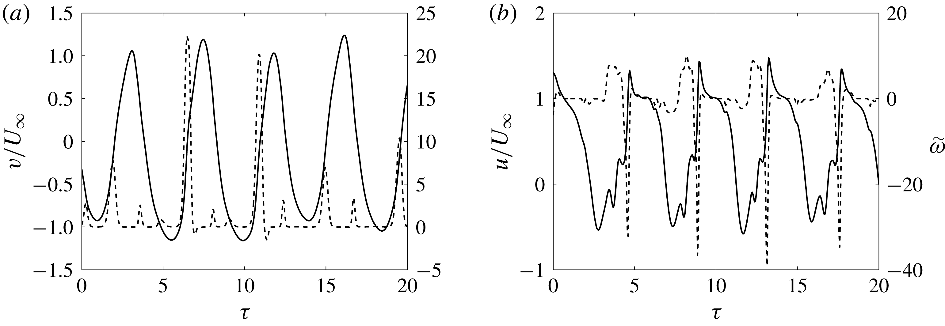
negative vorticity diffuses into the fluid interior from the solid boundary of the cylinder. When coherent structures with a negative vorticity are advected towards the upper boundary of the cylinder, it is possible for this vorticity to penetrate into the boundary layer, which will result in the flow decelerating to zero (figure 13
a). In contrast when positive vorticity is advected towards the upper part of the cylinder it is deflected away from the cylinder and the flow near the boundary is not accelerated. This is reflected in the time series of the point
 $\boldsymbol{x}_{2}$
which shows that there can be significant negative vorticity peaks (e.g.
 $\unicode[STIX]{x1D70F}=7$
and
 $\unicode[STIX]{x1D70F}=15$
) which results in the tangential velocity decreasing to zero. However, there is no significant positive vorticity peak at this point with the potential to accelerate the flow.
Time series of the (a) cross-stream and (b) streamwise velocity (full line) and non-dimensional vorticity (dashed line) at the positions (a)
 $\boldsymbol{x}_{1}/D_{G}=\{-0.57,0\}$
and (b)
 $\boldsymbol{x}_{2}/D_{G}=\{0,0.57\}$
for viscous simulations with an upstream cylinder. In (a) the velocity fluctuates in the positive and negative directions equally due to the passage of positive and negative vortices. In (b) the horizontal velocity is only decelerated (never accelerated) as the positive vortices are not able to penetrate into the boundary layer.

7.3 Internal and near field wake
7.3.1 Mean flow
The streamline plots in figure 7 show that the arrays
 $N_{133}$
and
 $N_{95}$
are behaving similarly to the solid cylinder case
 $N_{S1}$
as they also have large recirculating regions downstream of the arrays. From a topological perspective, the case of
 $N_{S1}$
, results in four half-saddle points (on the cylinder surface), two nodes (within the flow) and a downstream saddle point which is consistent with the analysis given in Hunt et al. (Reference Hunt, Abell, Peterka and Woo1978). The recirculating regions of
 $N_{133}$
and
 $N_{S1}$
are of a comparable length and width however it is much narrower for the case of
 $N_{95}$
due to the effect of the increased streamwise and lateral bleed. This additional flow also displaces the stagnation point further downstream as is highlighted in figure 7(b,c). The streamlines also indicate that the recirculating region extends into the array from the downstream side; an effect that will also be seen in the forces experienced by the cylinders at the back of the array. This also contrasts with the recirculation bubbles seen in the steady incident flow condition in Chang & Constantinescu (Reference Chang and Constantinescu2015). This type of mean flow for the high solid fraction arrays will have a profound effect on scalar transport as will be discussed later.
For the arrays with a solid fraction less than
 $N_{64}$
, the bleed through the array is sufficient to prevent recirculation regions. As the solid fraction is decreased the drag due to the cylinders also decreases which results in a faster flow within the array and in the wake of the array (figure 7
b–h). The width of this slow moving region is shown in blue in figure 7(d–f) which visibly narrows as
 $\unicode[STIX]{x1D719}$
decreases. Especially for the case of
 $N_{7}$
and
 $N_{1}$
the effects of the cylinders is very localised and there is minimal interaction between the cylinders. Additionally, as the array has little effect on the large vortices, they move through the array unchanged, resulting in the individual cylinders shedding obliquely in alternating directions at
 $\unicode[STIX]{x1D703}\approx \pm 30^{\circ }$
which can be seen in a decrease of the speed at this angle (shown in yellow in figure 7
g,h).
For arrays with cylinders in a steady flow, Nicolle (Reference Nicolle2009) found that for low
 $\unicode[STIX]{x1D719}$
there were clear recirculation regions behind the individual cylinders. However, for high
 $\unicode[STIX]{x1D719}$
, it was found that the flow resembles that of a potential flow through the array which was also seen in the high Reynolds number three-dimensional simulations of Moulinec, Hunt & Nieuwstadt (Reference Moulinec, Hunt and Nieuwstadt2004). In the current simulations, due to the advection of positive and negative vorticity past the array the average flow also resembles that of a potential flow, even at low
 $\unicode[STIX]{x1D719}$
.
7.3.2 Second order statistics
There are three main sources of unsteadiness in this problem; (i) the unsteadiness of the incident large vortices, (ii) the shedding of the vortices from the individual cylinders and (iii) the shedding from the array itself (only present for the high solid fraction arrays). The main source of unsteadiness of the internal cylinders is the upstream wake but these large scale vortices find it increasingly difficult to penetrate into the array for a higher solid fraction. Figure 14 shows the internal second order statistics of the velocity field with distance into the array. The general trend is that the higher the solid fraction of the array, the greater the decrease in these second order statistics with the normal component decreasing significantly more than the cross-stream component. Blocking in front of the cylinder has already decreased this velocity component significantly (before the fluid enters the array).
7.4 Rapid distortion theory
One possibility of modelling the interaction of an inhomogeneous unsteady flow with an array of obstacles is rapid distortion theory (RDT). Hunt (Reference Hunt1973) analysed the flow of a homogeneous turbulent flow past a cylinder which we shall extend to the flow past an array of circular cylinders.
Streamwise profiles of the r.m.s. of the (a) normal and (b) tangential velocity components for the viscous simulations with an upstream cylinder present, showing the decay of the fluctuations through the array. The different solid fractions are represented by
 $N_{0}$
(◃); 1 (▹);
 $N_{7}$
(○);
 $N_{20}$
(
 $+$
);
 $N_{39}$
(*);
 $N_{64}$
(
 $.$
);
 $N_{95}$
(
 $\times$
);
 $N_{133}$
(▫).

Non-dimensional vorticity plots for the RDT calculations for (a)
 $N_{S1}$
, (b)
 $N_{133}$
and (c)
 $N_{95}$
showing the distortion of the vorticity field around the arrays. The profiles of the r.m.s. in the tangential velocity component shown in figures 16, 18 and 19 are given by black dashed lines.

7.4.1 Fully blocked cylinder (case
$N_{S1}$
)

Figure 15(a) shows the RDT interaction of a vortex in front of a fully blocked cylinder. The decrease in the streamwise velocity immediately upstream of the cylinder (figure 8
a) results in the vorticity slowing down significantly and the favourable rate of strain in the mean streamwise velocity component (
 $|\unicode[STIX]{x2202}\bar{u}/\unicode[STIX]{x2202}y|>0$
) distorting the top and bottom of the vortex around the cylinder.
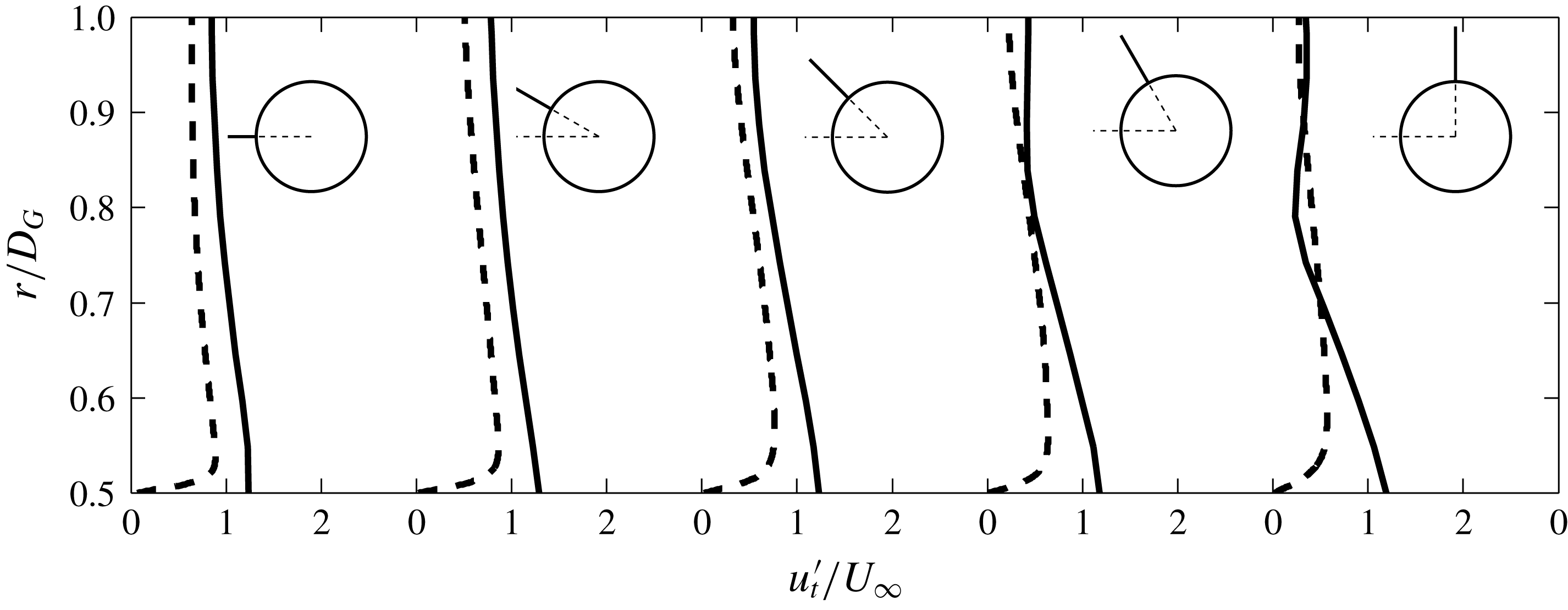
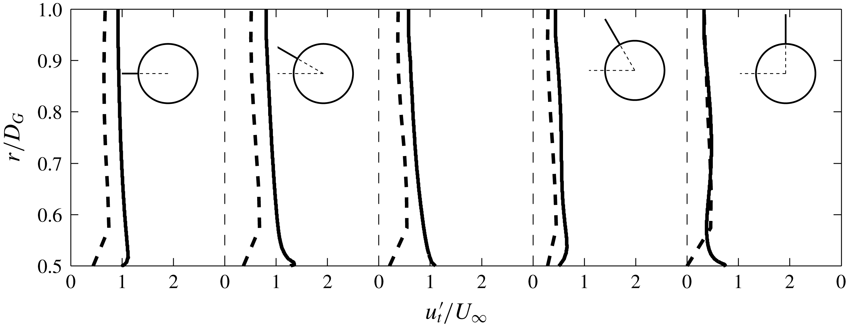
To show the effect of the vorticity distortion on the velocity statistics close to the cylinder, radial profiles of the r.m.s. of the tangential velocity, at various angles in front of the cylinder are plotted in figure 16. The modification of
 $u_{t}^{\prime }$
is greatest over
 $O(D_{G})$
and so, this gives the extent of the profile shown.
 $u_{t}^{\prime }|_{r/D_{G}=1}$
varies for the profiles as the free stream value of
 $u_{t}^{\prime }$
decreases with cross-stream location (i.e. the wake model given by (3.10)).
 $u_{t}^{\prime }$
increases in close proximity to the cylinder and this increase is independent of the angle at which the profile is taken. As this is different to the viscous simulations, the velocity and vorticity are again recorded at the points (
 $\boldsymbol{x}_{1}=\{-0.57,0\}$
) and side (
 $\boldsymbol{x}_{2}=\{0,0.57\}$
). Figure 17(a,b) shows that positive and negative patches of vorticity can penetrate close to the upper cylinder boundary which results in the flow at the point
 $\boldsymbol{x}_{2}$
accelerating and decelerating by a similar magnitude as point
 $\boldsymbol{x}_{1}$
(figure 17
e,f).
7.4.2 Effect of porosity
Figures 15(b) and 15(c) show the interaction of a patch of vorticity with the arrays
 $N_{133}$
and
 $N_{95}$
, respectively. The vorticity is severely distorted as it moves through the array due to the difference in travel time along adjacent streamlines which is dependent on the local distribution of the cylinders. This is most pronounced when the vortex moves partially through the array, resulting in the high relative speed between vorticity moving along streamlines within and outside of the array (figure 15
b).
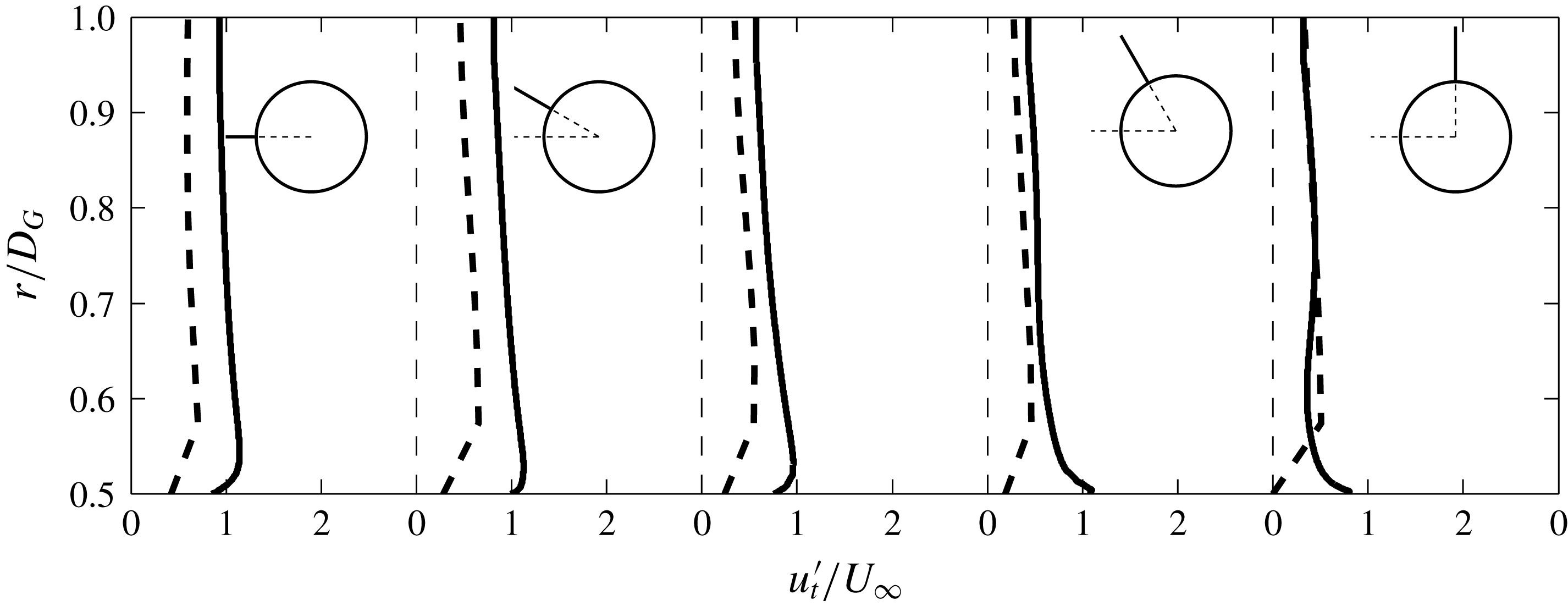
The profiles of the variation of the r.m.s. of the tangential velocity are shown in figures 18 and 19 for the arrays
 $N_{133}$
and
 $N_{95}$
, respectively. Here
 $u_{t}^{\prime }|_{r/D_{G}=1}$
is similar for the arrays as for
 $N_{S1}$
as the same wake model is used. The profiles for the two arrays are quite similar even though there is a difference in the solid fraction of 0.1, however the variation of the profile at a distance
 $O(D)$
from the array is largely dependent on the local geometrical layout of the array. The location of these profiles can be seen in figure 15(b,c). For example for
 $N_{133}$
the amplification at
 $\unicode[STIX]{x1D703}=4\unicode[STIX]{x03C0}/6$
is much greater than
 $\unicode[STIX]{x1D703}=3\unicode[STIX]{x03C0}/4$
due to the close proximity of the cylinder in the profile at
 $\unicode[STIX]{x1D703}=4\unicode[STIX]{x03C0}/6$
.
Radial profiles of the r.m.s. of the tangential velocity field in the vicinity of the array
 $N_{S1}$
for viscous simulations with an upstream cylinder (dashed lines) and inviscid RDT calculations (black lines).

Non-dimensional vorticity plots for the inviscid RDT calculations for the case
 $N_{S1}$
at
 $\unicode[STIX]{x1D70F}=$
(a) 2.38, (b) 3.57, (c) 7.14 and (d) 11.9. The vorticity field ranges from
 $-10$
(blue) to 0 (green) to 10 (red). Time series of the velocity (full line) and vorticity (dashed line) at the positions (e)
 $\boldsymbol{x}_{1}/D_{G}=\{-0.57,0\}$
(grey marker) and (f)
 $\boldsymbol{x}_{2}/D_{G}=\{0,0.57\}$
(black marker). In (a) the velocity fluctuates in the positive and negative direction equally due to the passage of positive and negative vortices. In (b) the horizontal velocity is both accelerated and decelerated. These inviscid results are in contrast to the previous viscous simulations shown in figure 13.

Radial profiles of the r.m.s. of the tangential velocity field in the vicinity of the array
 $N_{133}$
for viscous simulations with an upstream cylinder (dashed lines) and inviscid RDT calculations (black lines).

Radial profiles of the r.m.s. of the tangential velocity field in the vicinity of the array
 $N_{95}$
for viscous simulations with an upstream cylinder (dashed lines) and inviscid RDT calculations (black lines).

7.5 Applicability of RDT
The differences which were found in the DNS and RDT calculations need to be explored. The mean flow field for the RDT calculations was taken to be the irrotational flow through and around the array. As has been highlighted in Hunt (Reference Hunt1973), even for steady incident flow conditions and
 $u^{\prime }/U_{\infty }\ll 1$
this assumption is still only approximate as the wake affects the flow in this region. In this study
 $u^{\prime }/U_{\infty }\sim 1$
and the nature of the incident wake (i.e. an oscillating von Kármán vortex street) had the effect that the mean streamwise deceleration in front of the cylinder was significantly greater than for the potential flow (figure 8
c). An additional consequence of
 $u^{\prime }/U_{\infty }\sim 1$
is that the upstream vorticity will not necessarily move along the mean streamline (an assumption of RDT). For
 $\unicode[STIX]{x1D719}<1$
the upstream strain field is modified due to the effect of viscous drag resulting in a significantly reduced mass flux through the array leading to differences in the parameters
 $\unicode[STIX]{x1D6E5}_{T}$
and
 $\unicode[STIX]{x1D6E5}_{Y}$
. Therefore patches of vorticity in the viscous simulations will have a greater tendency to be moved around the array than through the array. Additionally, the effect of the viscous interaction between the vortex and the cylinder (i.e. secondary vorticity generation) is not captured in the RDT calculation which will affect the residence time of the vortex in the vicinity of the cylinder.
8 Forces on the array
In this section the effect of varying the solid fraction on the forces exerted on the individual cylinders and the group as a whole is investigated. For low solid fraction arrays a method of calculating the forces on the cylinders is demonstrated.
8.1 Forces acting on individual cylinders in array
Figure 20 shows plots of the force characteristics on individual cylinders for the different solid fractions. The mean force coefficient at the mean force angle is given by the black line and the red lines are the range of the r.m.s. of the force angle. To give an indication of the r.m.s. of the force coefficient of the individual cylinders, the background of each cylinder shows the ratio of the r.m.s. of the force coefficient to the mean of the r.m.s. of the force coefficient of all of the cylinders in the array (i.e.
 $C_{iT}^{\prime }/\bar{C^{\prime }}_{iT}$
).
Plots of the mean force coefficient at the mean force angle (black line) and the range of the r.m.s. of the force angle (red lines – note it does not represent magnitude) for each cylinder. The line at the bottom left of each figure represents a force coefficient of unity. The ratio of the r.m.s. of the force coefficient on an individual cylinder to the mean of the r.m.s. of the force coefficients for the cylinders in the array (
 $C_{Ti}^{\prime }/\bar{C^{\prime }}_{Ti}$
) is shown as the background colour of each cylinder. The arrays are: (a)
 $N_{133}$
(0.12), (b)
 $N_{95}$
(0.17), (c)
 $N_{64}$
(0.24), (d)
 $N_{39}$
(0.40), (e)
 $N_{20}$
(0.62) and (f)
 $N_{7}$
(0.83) where the value in brackets is the mean of the r.m.s. of the force coefficients for all the cylinders in the array (
 $\bar{C^{\prime }}_{Ti}$
). The flow is from left to right.

For the higher solid fraction arrays the effect of blocking and drag is significant and results in a greatly reduced mean total force coefficient on the front cylinders of the array and shielding results in a decrease of the cylinder force coefficient with distance through the array. The r.m.s. of the force on the frontal cylinders also decreases which is because the velocity fluctuations in front of the array increase with decreasing solid fraction (see figure 9). The r.m.s. of the total force on the frontal cylinders is much greater than that of the central cylinder (a factor of 4 for the case of
 $N_{133}$
). This is because the large vortical structures cannot penetrate far into the array and also the individual cylinders shear layers all reattach to the next downstream cylinder, thereby suppressing vortex shedding (figure 3 shows no presence of small scale vorticity in the larger vortical structures for the high solid fraction arrays). For the case of
 $N_{133}$
and
 $N_{95}$
the force angle for the individual cylinders at the back of the array is reversed as the collective effect of the cylinders is to behave similar to a single solid body and shed vortices. Similar features were seen in Nicolle & Eames (Reference Nicolle and Eames2011).
For the case of
 $N_{39}$
and
 $N_{20}$
the interaction between cylinders and the cylinders and the upstream wake is weaker. The decreased effect of blocking results in an increased average incident velocity on the front cylinders of the array, resulting in an increased total force coefficient for these cylinders (compared to the high solid fraction arrays). The spacing between the cylinders is,
 $\unicode[STIX]{x1D706}/D\approx 4$
, which means that the flow can alternate between vortex shedding and reattachment to the next downstream cylinder. This can be seen in figure 5 as there are not as many intense vortices downstream of the array. The flow between the individual cylinders does not recover and there is a noticeable drop in the mean and r.m.s. of the force coefficients through the array (i.e. shielding). These trends are greater for
 $N_{39}$
than
 $N_{20}$
.
For the low solid fraction cases,
 $N_{1}$
and
 $N_{7}$
, there is weak interaction between the cylinders. For the case
 $N_{1}$
,
 $C_{1TG}\approx 0.1$
which is the equivalent of
 $C_{1T}\approx 2.1$
. The effect of blocking is not significant for these arrays, however there is still a reduction in the force coefficient of the front cylinders (of
 $N_{7}$
) of approximately 15 % (compared to an isolated cylinder). The large vortical structures move through the array unobstructed and for
 $N_{7}$
the separation distance between cylinders is,
 $\unicode[STIX]{x1D706}/D\gg 1$
, which means that all the cylinders are shedding vortices (see figure 6) and the flow nearly recovers before it is incident on the downstream cylinders resulting in similar but slightly reduced mean total force statistics.
Time series of the (a,c) total group force coefficient
 $C_{TG}$
and (b,d) force angle
 $\unicode[STIX]{x1D703}_{|\boldsymbol{F}|G}$
for (a,b)
 $N_{c}=1$
(full black),
 $N_{7}$
(dashed black),
 $N_{20}$
(full grey) and
 $N_{39}$
(dashed grey) and (c,d)
 $N_{64}$
(full black),
 $N_{95}$
(dashed black),
 $N_{133}$
(full grey) and
 $N_{S1}$
(dashed grey). The variation of the mean (○) and r.m.s. (
 $\times$
) of (e)
 $C_{TG}$
and (f)
 $\unicode[STIX]{x1D703}_{|\boldsymbol{F}|G}$
with solid fraction
 $\unicode[STIX]{x1D719}$
. The dashed black and grey line indicate the mean and r.m.s. for
 $\unicode[STIX]{x1D719}=1$
, respectively. The prediction using the model described in § 3.2 is shown for the mean (▹) and r.m.s. (◃) of
 $C_{TG}$
and
 $\unicode[STIX]{x1D703}_{|\boldsymbol{F}|G}$
, respectively.

Relative position of the cylinders for (a)
 $N_{20}$
and (b)
 $N_{133}$
with their index given within the circle. The dashed line in (a) and (b) indicates the cylinders which have a correlation coefficient higher than 0.7 with
 $N_{20,19}$
(the first subscript denotes array type and the second indicates the individual cylinder) and
 $N_{i}=126$
respectively. Contour plots of the correlation coefficient between the cylinders in the array for (c)
 $N_{20}$
and (d)
 $N_{133}$
. The upper half is the total force and the lower half is the force angle, which are divided by the solid black line. The dashed line in (d) indicates the correlation coefficients for
 $N_{133,126}$
. The flow is from left to right.

The time series of the angle of the force for
 $N_{1}$
in figure 21(b) shows that the single cylinder experiences two frequencies. Firstly, the cylinder is shedding vortices which is the higher frequency. Between
 $136<\unicode[STIX]{x1D70F}<140$
, the shedding frequency varies between 4 and 5 which is due to the unsteady local incident Reynolds number. This is higher than the frequency of vortex shedding of the upstream cylinder which is
 ${\approx}0.2$
. This lower frequency is observed in all the arrays figure 21(b,d).
In the steady incident flow simulations (Nicolle & Eames Reference Nicolle and Eames2011; Chang & Constantinescu Reference Chang and Constantinescu2015) it was found that for the higher solid fractions (
 $N_{39}$
and above) the force on the cylinders was much greater at
 $\unicode[STIX]{x1D703}\approx \pm 130^{\circ }$
than at the front of the array (i.e.
 $\unicode[STIX]{x1D703}=180^{\circ }$
). This is due to the effect of blocking of the cylinders decelerating the oncoming flow and the fluid accelerating around the side of array. The effect of the inhomogeneous flow in the present simulations is that
 $\bar{C}_{Ti}$
is greatest for the cylinders located between
 $\unicode[STIX]{x1D703}\approx \pm 130^{\circ }$
which have approximately similar total force coefficients.
8.2 Group force
The trends in the total group force and angle coefficient will be described and then the statistics of the individual cylinders will be analysed to give insight into these trends. Figure 20 shows the variation of the mean total force coefficient with solid fraction. For the cases
 $N_{7}$
,
 $N_{20}$
and
 $N_{39}$
(compared to
 $N_{1}$
), the increased effect of blocking and shielding results in a less than linear response of the mean group force coefficient. This effect becomes greater with increasing solid fraction and all the arrays have a mean force coefficient less than the solid array case
 $N_{S1}$
. The effect of the individual cylinders shedding vortices can be seen in the time series in figure 21(a,b) which is suppressed in the high solid fraction arrays (figure 21
c,d).
The behaviour of the r.m.s. of the group total force can be roughly split into low (
 $N_{39}$
and below) and high solid (
 $N_{64}$
and above) fractions, which is shown in figure 21(c). There are three potential sources of unsteadiness in this problem, namely (i) the unsteadiness due to the upstream wake, (ii) the unsteadiness of the individual cylinders in the array shedding vortices and for the high solid fraction arrays and (iii) the unsteadiness of the array acting as a solid body and shedding vortices.
For low
 $\unicode[STIX]{x1D719}$
, the individual cylinders have a similar high r.m.s. (e.g. for
 $N_{20}$
,
 $\bar{C^{\prime }}_{Ti}=0.62$
), however there is a low correlation between the forces on these cylinders. For example the front cylinder
 $N_{i}=19$
is only well correlated (i.e. a correlation coefficient greater than 0.7) to two other cylinders (figure 22
a,c) resulting in
 $C_{TG}^{\prime }\approx 0.35$
. In contrast, for solid fraction arrays of
 $N_{64}$
and above,
 $C_{TG}^{\prime }\approx 0.55$
. As the solid fraction increases the average r.m.s. of the individual cylinders decreases (for
 $N_{133}$
,
 $\bar{C^{\prime }}_{Ti}=0.12$
) however the correlation between the cylinders increases. The dashed horizontal line in figure 22(c) indicates the correlation of cylinder
 $N_{133,126}$
(the first subscript denotes array type and the second indicates the individual cylinder) with all the other cylinders in the array. The cylinders that are well correlated are shown in figure 22(b). These are the cylinders which also have the highest individual r.m.s. of the force coefficient (figure 20
 $f$
). The central cylinders and the cylinders to the rear have a relatively low fluctuating force component.
The mean force angle is zero due to the (near) symmetrical arrangement of the cylinders and the upstream cylinder sheds vortices of a similar strength but opposite sign in a periodic fashion. The low solid fraction arrays have high frequency oscillations in the force angle not seen in the high solid fraction arrays which is due to individual cylinders in the low solid fraction arrays shedding vortices. This is suppressed in the high solid fraction arrays. The force angle becomes increasingly correlated for more cylinders as the solid fraction increases, which can be seen in the lower halves of figure 22(c,d). The arrays
 $N_{95}$
and
 $N_{133}$
have the additional unsteadiness associated with the array acting like a single body and shedding vortices, however it was not possible to discriminate this effect.
8.3 Estimation of the force on cylinders for
$\unicode[STIX]{x1D719}\ll 1$

The cylinder elements of the array are removed and the numerical simulation is repeated (i.e. case
 $N_{0}$
) and velocity statistics are recorded at the centre of the removed cylinders. This is similar to the method of Bagchi & Balachandar (Reference Bagchi and Balachandar2003) for calculating the drag on a sphere in a turbulent flow. The drag, inertial and lift forces are then estimated using (3.12)–(3.15), respectively. For the case of
 $N_{1}$
, figure 21(e,f) shows that there is a good agreement between the mean and r.m.s. of the force coefficients and angle calculated using this method and the full viscous numerical simulation with the cylinder present. This procedure can also be carried out for
 $N_{7}$
and
 $N_{20}$
. In figure 21(e,f) we can see that the force characteristics are well predicted for
 $N_{7}$
. However, as the interaction between the cylinders increases, as is the case for
 $N_{20}$
, this method will start to overpredict the force on cylinders which are towards the back of the array. This is due to a process called shielding whereby the drag coefficient of downstream cylinders is less than that with a uniform incident flow. This is due to the modification of the local velocity field by the upstream cylinder, which cannot be taken into account using the simulation
 $N_{0}$
.
9 Discussion and conclusions
In this study we have looked at the unsteady inhomogeneous flow through and around an array of circular cylinders of varying solid fraction. Returning to the questions posed in the introduction, the combination of inviscid blocking and viscous drag leads to the modification of the upstream mean streamwise velocity and strain field. The mean mass flux through the array is decreased with increasing solid fraction and two recirculation regions are present in the near wake for high solid fraction arrays. For the high solid fraction arrays, the incident vorticity is slowed down in front of the array and the tangential velocity component is amplified. As a means of extrapolating to very high Reynolds numbers, rapid distortion theory (RDT) calculations were carried out. These calculations highlighted that the tangential velocity will be amplified, equally, at the front and sides of the array which was not found for the finite Reynolds number numerical simulations.
The ability of the unsteady incident flow to penetrate into the array reduces significantly with increasing solid fraction. This has a profound influence on the second order statistics within the array which directly affects the forces on the cylinders. For low solid fraction arrays (
 $N_{20}$
and less), where the interaction between the individual elements and the individual elements and the incident flow is weak, the total force on the cylinders and the group force can be estimated by decomposing the total force into drag, inertial and shear induced lift components. These contributions can be estimated by repeating the simulation with all the cylinders removed and taking the velocity statistics at the centre of the removed cylinders. As the solid fraction increases there will be two effects, the collective action of the cylinders increases, resulting in a reduced incident flow on the upstream cylinders. Also the upstream cylinders will result in a modified flow on the downstream cylinders, commonly known as shielding. Both of these elements are not captured in the model and so these methods can only be used for
 $\unicode[STIX]{x1D719}\ll 1$
. For
 $N_{64}$
and above, the r.m.s. of the group force becomes insensitive to the solid fraction. This is because although the average r.m.s. of the force of the individual cylinders decreases (with increasing
 $\unicode[STIX]{x1D719}$
), there are more of them and they are more correlated (due to their close proximity).
Accurately predicting the flow through and around structures is essential in being capable of predicting the loading on structures. Depending on the application, the physics present in the flow can vary dramatically. For example when studying the loading on members in the offshore sector the incident flow will be oscillatory, a combination of waves and current. Inundation due to tsunamis and storm surges will have unsteady free surface flows. Although these flows are quite different, the general mechanism of why the incident flow is modified by individual members or the collective action of the structure as a whole is common to both and decomposing this effect into inviscid blocking and viscous drag is one of the key outcomes of this paper.
The effect of accurately modelling this inviscid blocking and viscous drag is important in applications such as dispersion of organic waste due to caged farmed fish (where the cages can be approximated to a region with porosity) in the upper part of the water column (Wu et al. Reference Wu, Chaffey, Law, Greenberg, Drozdowski, Page and Haigh2014). Again if the inviscid shallow water equations are used to model the flow due to tides or rivers, the effect of viscous drag needs to be included to ensure that, firstly, the mass flux through the array is accurately modelled and secondly, any recirculation regions behind the array are taken into account. A related problem is that of pollutant dispersion as flows encounter an array of emergent vegetation (Nepf Reference Nepf1999).
To begin to understand the effect that extending this work to three dimensions would have, three-dimensional calculations were carried out of the same geometries with a spanwise extrusion of
 $10D$
. The key difference between the two- and three-dimensional simulations was that during and after the interaction with the array the coherence of the vortices (shed by the upstream cylinder) in three dimensions was much less. Conversely, the interaction between the vortices and the array (and individual cylinders) is much stronger in two dimensions. The quantitative effect is that the total group force for the arrays is overestimated in the two-dimensional simulations. Additionally, the range of the r.m.s. of the force angle of the individual cylinders throughout the array was not as great for the three-dimensional simulations. Qualitatively the only difference between the two- and three-dimensional simulations was that the negative force on the individual cylinders at the back of the array was not observed in three dimensions. The other trends of the force and force angle which were discussed in § 8 were similar in both simulations. This highlights the utility of using two-dimensional simulations for this fundamental study. Further work is required to fully understand this three-dimensional interaction.
Acknowledgements
C.A.K. and I.E. acknowledge support from the European Research Council under the European Union’s Seventh Framework Programme (FP7/20072013)/ERC grant agreement no. 336084, awarded to Professor T. Rossetto (UCL). The authors acknowledge the use of the UCL Grace High Performance Computing Facility (Grace@UCL), and associated support services, in the completion of this work.