

Introduction
Variation is inherent in biology. Animals and plants are variable in their habitats, behaviors, and morphology. This variation can be hereditary and can be used in taxonomy, systematics, and phylogenetics; it can be induced by environmental effects and can be useful in ecology and paleoenvironmental studies; or it can arise from a mix of these factors. Regardless of its origins, identifying and quantifying morphological variation is the first step to understanding and using it.
Geometric morphometric methods quantify biological shape using mathematical tools (e.g., Zelditch et al. Reference Zelditch, Swiderski, Sheets and Fink2004; Webster and Sheets Reference Webster and Sheets2010) and may be applied to a wide spectrum of organisms and biological questions (e.g., Zelditch et al. Reference Zelditch, Bookstein and Lundrigan1992, Reference Zelditch, Sheets and Fink2000; Fink and Zelditch Reference Fink and Zelditch1995; Monteiro et al. Reference Monteiro, Di Benetto, Guillermo and Rivera2005; Aguirre et al. Reference Aguirre, Perez and Sirch2006, Reference Aguirre, Richiano, Alvarez and Farinati2016; Clouse et al. Reference Clouse, de Bivort and Giribet2009; de Bivort et al. Reference de Bivort, Clouse and Giribet2010; Klingenberg and Gidaszewski Reference Klingenberg and Gidaszewski2010; Collins et al. Reference Collins, Crampton and Hannah2013, Reference Collins, Crampton and Hannah2014). Underpinning most geometric morphometric studies is a set of photographs of the specimens being studied; however, photographs of objects are inevitably imperfect representations of those objects. Optics, such as camera lenses, will distort an image to some extent when a photograph is taken. The extent of the distortion will depend primarily on factors such as the make and model of the lens (and camera) but also on user-controlled factors such as the zoom of the lens, the f-stop (aperture), shutter speed, and placement of the object within the field of view. Thus, any study that uses a configuration of landmarks and/or semilandmarks digitized from a photograph (e.g., Bookstein Reference Bookstein1991, Reference Bookstein1997; Zelditch et al. Reference Zelditch, Swiderski, Sheets and Fink2004; Perez et al. Reference Perez, Bernal and Gonzalez2006; Webster and Sheets Reference Webster and Sheets2010; Collins et al. Reference Collins, Crampton and Hannah2013, and many others) will have shape variation introduced to the data set by the camera. That error may be statistically relevant, depending on specifics of the photographic method and the taxa under study.
To our knowledge, there has yet to be a study that has tested the significance of the inherent error associated with photographing specimens and the effect this has on morphometric analyses. We offer an example using a set of 30 bivalve shells of various sizes from a single clade, imaged using a single camera and lens, to demonstrate the potential magnitude of the error associated with photographing specimens, and methods that may help minimize that error.
Lens Distortion
A photograph is a two-dimensional (2D) representation of a specimen that in almost all cases is substantially three-dimensional (3D), and there is distortion involved in projecting a 3D shape to a plane (Arnqvist and Martensson Reference Arnqvist and Martensson1998). The mactrid data set presented here consists of landmarks taken from a shallow concave surface and projected to the sagittal plane of the animal. The landmarks and semilandmarks used here fall on or close to the margin of the shell, that is, as close to lying on the sagittal plane as possible. In choosing to proceed with 2D rather than 3D morphometrics, investigators accept this source of error and assume that it is trivial relative to biological variation, as we have done with the present data set. Whether or not this assumption is valid in any given case, camera and lens-related distortion effects will only further compound this inherent error.
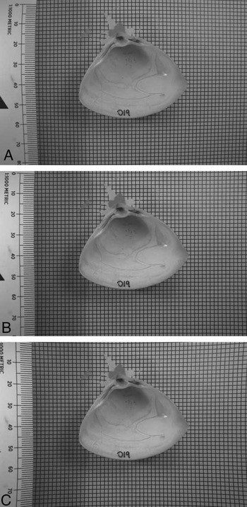
There is an abundant literature on the mathematics of lens distortion, although a review of this is well beyond the scope of this paper. Interested readers are directed to Cox (Reference Cox2007) for a recent summary. In brief, however, there are two main kinds of distortion caused by lenses. Barrel distortion is a lens property that causes the center of straight lines to bow out toward the edges of the image; while pincushion distortion has the opposite effect, causing the center of straight lines to bend inward. The lens and camera setup we used produced barrel distortion to varying degrees but no pincushion distortion. Figure 1 shows a raw image from our data set that exhibits strong barrel distortion, its digitally retrodeformed counterpart, and the same image digitally altered to simulate pincushion distortion. It is immediately apparent that distortion is greatest closest to the edges of the frame—which is typically where the scale bar is placed in morphometric images. This issue has been noted by previous authors in the morphometric literature, most recently by Muir et al. (Reference Muir, Vecsei and Krueger2012), whose recommendation is to use a camera of more than 5 megapixels with a lens with a focal length greater than 35 mm. Careful selection of appropriate equipment and photographic setup will help minimize error from the outset, it is true, but even the best equipment is not entirely free of lens distortion.
Effects of lens distortion. A, Raw image of a specimen of Crassula aequilatera sitting on top of a piece of grid paper. B, The same photo, digitally retrodeformed so that the grid behind the shell is returned to square. C, The same photo, digitally distorted to simulate pincushion distortion. Images A and B are taken from the data set used in this paper; image C was produced using Adobe Photoshop, as no pincushion distortion was produced by our photographic setup. The contrast level of the photos is as required to highlight and identify internal shell features for morphometric analysis.

It is, however, possible to correct for lens distortion by digital retrodeformation, using a reference photograph of grid paper and the inbuilt correction algorithms in software packages such as Adobe Photoshop. But this begs the question: Is this a standard step that should be undertaken before the digitization of landmarks? Or is the variation in the shape of the specimens being photographed significant enough that the error from lens distortion can be regarded as minimal and thus discounted? Given the amount of time that photographic processing and data capture for morphometric analyses takes, this is a nontrivial question. Adding a further step to the morphometric workflow will make it more time-consuming, but if the distortion induced by photography is significant, then not taking the time to retrodeform images would be remiss. It should also be noted that there are ethical issues associated with the manipulation of images (e.g., Cromey Reference Cromey2010). However, providing workers are transparent in what they have done to account for lens distortion and maintain copies of both raw and retrodeformed images, we do not feel that correction for lens distortion in morphometric data sets is ethically unsound.
This study aims to (1) ascertain the significance of distortion introduced using a single camera and various photographic methods and (2) recommend ways to minimize the effects of photographic distortion on shape analysis.
Materials and Methods
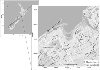
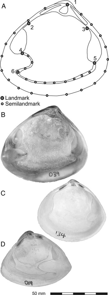
Thirty specimens from three species of New Zealand Mactridae (9 Mactra discors Gray, Reference Gray1837; 11 Cyclomactra tristis (Reeve, Reference Reeve1854); and 10 Crassula aequilatera (Deshayes in Reeve, Reference Reeve1854) (Fig. 3B, C, and D, respectively) were collected as dead shells by beachcombing from a 1 km transect (S 40°52′24″, E 174°59′52″ to S 40°52′38″, E 174°59′29″) along the Paraparaumu Beach shoreline south from Waikanae Estuary (lower North Island, New Zealand) (Fig. 2), over a period of 6 months. Mactrids were selected as a suitable study group for this investigation, because the various species are similar in terms of discrete anatomical characters such as teeth, muscle scars, sculpture, and so on, but distinctive and separable by overall shape. The analysis was restricted to Recent taxa in order to limit as much as possible the effect of taphonomy on shell shape.
Map of collection transect for mactrid data set. Base maps downloaded from Google Maps and plotted using R package ggmap (Kahle and Wickham Reference Kahle and Wickham2013).

Specimens were cleaned, dried, and numbered, and then the internal view was photographed. Digitization of landmarks and semilandmarks followed the method outlined in Collins et al. (Reference Collins, Crampton and Hannah2013). Configurations of landmarks and semilandmarks (Fig. 3) were captured using tpsDig (Rohlf Reference Rohlf2005). Landmarks were placed at the tip of the beak (1), the junction of the posterior and anterior muscle scars with the hingeplate (2 and 3, respectively), the junction of the posterior and anterior muscle scars with the pallial line (4 and 5, respectively), and the tip of the flexure between the pallial line and pallial sinus (6). These landmarks are consistently locatable across all specimens and represent anatomical features (junctions of tissues or structures with functions) rather than geometric points on the shape.
Morphometric setup and included species. A, The landmark/semilandmark configuration used in this study. Landmarks are numbered (see text). B, Mactra discors. C, Cyclomactra tristis. D, Crassula aequilatera. Scale bar applies to B–D only.

The outline of each specimen was captured as a closed curve of 19 semilandmarks anchored on landmark 1 (total points: 20). The pallial line (minus the pallial sinus) was captured as an open curve using landmarks 5 and 6 as endpoints, with eight semilandmarks in between (total points: 10); and the pallial sinus was captured as an open curve using landmarks 6 and 4 as endpoints, with three semilandmarks in between (total points: 5). The number of semilandmarks for each curve was chosen as the fewest number of points required (by visual estimation) to capture that curve.
Landmarks are discrete anatomical loci, and sets of configurations composed only of landmarks can be put directly into Procrustes superimposition. Semilandmarks, however, are not discrete loci but instead collectively describe a curve. Their individual spacing along that curve is not biologically meaningful, but if semilandmark sets are digitized and then immediately subjected to Procrustes superimposition, subsequent analyses will assume that their position is important, and any difference in that position between specimens will be treated as equally important to the difference in position between real biological landmarks. To minimize this issue, after digitizing but before Procrustes superimposition is performed, semilandmarks are slid computationally along their curves to minimize the difference in shape between the specimens in the data set. In the present study, these operations were performed in R (R Core Team 2016) using the package geomorph (Adams and Otárola-Castillo Reference Adams and Otárola-Castillo2013). A more in-depth explanation of landmark and semilandmark methods can be found in Webster and Sheets (Reference Webster and Sheets2010).
Four photographic settings were used to image each specimen. The parameters of each photographic setting are listed in Table 1. To keep the parameters of the data presented in this paper as simple as possible, a single camera (Nikon D800) and a single lens (Nikkor 24–85 mm, f 2.8–4.0) were used throughout. The Nikon D800 is a 36 megapixel, full-frame digital single-lens reflex (SLR) camera; significantly, it allows the user to switch the camera between full-frame (35 mm image sensor) and crop-sensor mode (the sensor size in most modern digital SLR cameras), using in-camera settings. This Nikkor lens has a built-in macro function, allowing the focal lengths required for macro photography to be achieved; however, this limits the available zoom to 35–85 mm. The specimen and the camera tripod were not moved in between photographs, but the camera height and settings were adjusted to ensure the shell was maintained at a similar size in the frame (Table 1).
Camera setup. All photographs were taken using a Nikon D800 with a Nikkor 24–85 mm, f 2.8–4.0 lens at ISO 100 and f 25. Camera set to aperture priority, shutter speed varied from 1/5 s to 1/1.6 s. Each raw photo has an undistorted counterpart.

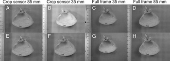
The four sets of photographs were then subsequently retrodeformed using the Lens Correction filter in Adobe Photoshop, with the square grid paper that each specimen was photographed on top of as a reference. These four sets of retrodeformed images were then digitized in the same manner as the raw photographs. Figure 4 shows the eight different images of specimen 019 (Crassula aequilatera). The differences are subtle but clearly detectable by the human eye. It is important to note that other software capable of lens correction is available, for example, View NX, produced by Nikon; GIMP; and plug-ins for Irfanview (the latter two are freeware). We chose to use Adobe Photoshop simply because it was the method with which we were most familiar. Testing the capability of other software, although an interesting exercise, is outside the scope of the present study. If the retrodeformation step was effective, retrodeformed images of a single specimen would produce landmark configurations that are more similar to each other than those produced by a set of raw images; one would expect the set of retrodeformed images to have lower Procrustes variance than the set of raw images for any given specimen, and we would expect to see the landmark configurations digitized from those images clustering more tightly than those from the corresponding raw photos in ordinations.
Eight individual images of a single specimen of Crassula aequilatera. A–D are raw images, straight from the camera, with no correction of any kind. E–H were retrodeformed digitally but had no other corrections applied. The distance between camera and specimen changes between methods (Table 1). The contrast level of the photos is as required to highlight and identify internal shell features for morphometric analysis.

Human error and inconsistencies in the digitization process also are known sources of potential variance in any morphometric data set. To visualize the magnitude of this variance compared with that resulting from interspecific variation, we have followed the recommendation of Webster and Sheets (Reference Webster and Sheets2010), and using the subset of images of all specimens from a single method (85 mm full-frame, retrodeformed), plus five replicates of a single photograph of the same specimen of Crassula aequilatera (022) in the data set, we have compared the Procrustes variance that the replicates contribute versus the interspecific variance, using function morphol.disparity in R package geomorph (Adams and Otárola-Castillo 2013). We chose to do replicate digitizations of a single photo, rather than full remounting and photographing, because specimens were not moved or remounted during the experiment—only camera settings were changed between photographs of the same individual.
To assess how much variance in the data set is due to photographic method, we performed Procrustes analysis of variance (Procrustes ANOVA; also in geomorph, using function procD.lm, with residual randomization) on the full data set of raw and retrodeformed images. Procrustes ANOVA (Goodall Reference Goodall1991; Anderson Reference Anderson2001) is a nonparametric multifactorial ANOVA that evaluates sum of squares through permutation. Residual randomization produces higher statistical power and better pattern recognition (Anderson and Ter Braak Reference Anderson and Ter Braak2003). Procrustes variance was also used to examine the difference between raw and retrodeformed images specimen by specimen.
To illustrate a potential pitfall resulting from combining sets of images taken using different photographic parameters, we performed principal components analysis (PCA) and canonical variates analysis (CVA) on the raw images from the data set. CVA, a common technique in morphometric studies, is used to search for variance between groups assigned a priori, often coupled with PCA (e.g., Márquez et al. Reference Márquez, Robledo, Peñaloza and Van der Molen2010; Collins et al. Reference Collins, Crampton and Hannah2013; Gómez et al. Reference Gómez, Márquez, Gutiérrez, Conn and Correa2014), and is used to distinguish between, for example, putatively synonymous species, groups from different habitats, or samples from different stratigraphic horizons.
A subsidiary experiment was also undertaken to look for systematic effects caused by different levels of zoom. One specimen of Cyclomactra tristis (088) was photographed 22 times, at 11 different zoom levels at approximately 5 mm intervals, using both full-frame and crop-sensor modes. The camera, the specimen, and the scale bar were not moved during this experiment. The number of pixels occupied by the specimen in each photo increased with zoom level. All other photographic parameters remained constant (i.e., tripod setup, f-stop, shutter speed, position of specimen). No digital correction was applied to these images. In a crop-sensor camera, a limited field of view through the lens results from an image sensor that is not the same dimensions as 35 mm film, while the optics are designed for a 35 mm sensor/film. Smaller sensors in crop-sensor cameras result in a zoom factor being introduced, usually ~1.5×. In the D800 this is simulated by reducing the amount of the image sensor that is used to record the photograph. As this can be done within the camera, none of the setup needs to be altered or moved to swap cameras. Photographic settings for this experiment are also presented in Table 1.
Results
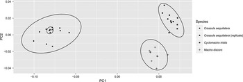
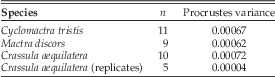
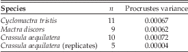
Examination of Procrustes variance indicates that digitization error is minimal compared with interspecific variation (Table 2). The magnitude of digitization error compared with interspecific variation can be visualized using PCA (Fig. 5).
PCA on specimens imaged using a single method (85 mm, full frame, retrodeformed), including five replicates of specimen 022. PC1 and PC2 account for 90% of the total variance in the data set (PC1=84.6%, PC2=5.6%).

Procrustes variance for species within the data set, using a single method (85 mm full frame, retrodeformed). A single image of specimen 022 was digitized five times (the specimen was not remounted and rephotographed; see text for explanation). The variance introduced by digitization error is an order of magnitude smaller than interspecific variation.
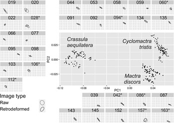
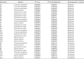
Procrustes ANOVA (Table 3) shows that photographic method has a statistically significant effect on mactrid shape, and Procrustes variance within each specimen for the raw photos versus the retrodeformed photos (Table 4) exhibits improvement (reduction of within-specimen variance) in 21 of 30 specimens for the retrodeformed images. To visualize this, we performed a PCA on the full data set (Fig. 6). Examined specimen by specimen (subplots within Fig. 6), 95% confidence ellipses on the mean principal component 1 (PC1) and principal component 2 (PC2) scores illustrate that retrodeforming images reduces the scatter caused by use of different photographic methods (Fig. 6).
PCA of the full mactrid data set. Individual specimens are shown in subplots (eight images each). Ellipses are 95% confidence intervals on the mean PC1 and PC2 scores of the raw (dashed line) and retrodeformed (solid line) image sets for each specimen. For clarity, individual point scatter is not shown within individual specimen plots. For most specimens, the retrodeformed images converge upon a mean shape more tightly than the raw images: any specimen for which this is not the case is indicated by an asterisk next to its sample number in the subplot header. PC1 and PC2 account for 89% of the total variance in the data set (PC1=82%, PC2=7%).

Results of Procrustes ANOVA (function procD.lm) on the mactrid data set. A randomized residual permutation procedure was used (1000 permutations). Type III (marginal) sums of squares and cross-products were used. SS, sums of squares; MS, mean squares.

Procrustes variance (PV) for specimens within the full data set, comparing variance of raw images (n=4) of each specimen with the variance of retrodeformed images (n=4) of the same specimen (total images per specimen=8). In 21 of 30 specimens, the variance of the retrodeformed images is less than that of the raw images.

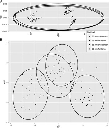
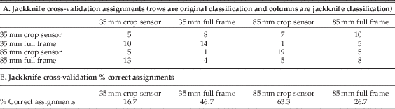
The effect of grouping images by photographic method rather than by species is illustrated by Figure 7, which shows the PCA of the raw images only, plotted by photographic method for display, and then the CVA of the same raw images, using photographic method as the grouping variable in the analysis. In the PCA, the photographic methods are indistinguishable—interspecific variation dominates both PC1 and PC2. However, the CVA has been forced to seek variance between the photographic methods, and it was able to do so, overriding the biological variation in the data set. Two of the groups in the CVA have entirely nonoverlapping 95% confidence ellipses on the group means. Table 5 gives jackknife cross-validation assignment scores and percentages of correct assignments. The CVA could not reassign images to photographic method groups all of the time, but the percentage of successful reassignments on one method (85 mm crop sensor) is greater than 60%, indicating that at least that method caused enough systematic variation in shape—distortion—for specimens photographed by that method to be united separately from specimens of the same species or images of the same specimen.
A, PCA on the raw images (4 photographic methods with no retrodeformations; 3 species; 30 specimens) from the full data set. Ellipses are 95% confidence intervals on the mean of each photographic method and are almost perfectly overlapping; photographic methods cannot be discriminated by PCA. PC1 and PC2 account for 88% of the total variance in the data set (PC1=81%, PC2=7%). B, CVA on the same data. Ellipses are 95% confidence intervals on the mean of each photographic method. Using CVA, it is possible to force discrimination between photographic methods, even though each method was applied to the same 30 specimens.

Results of CVA on raw images (n=30 per method).
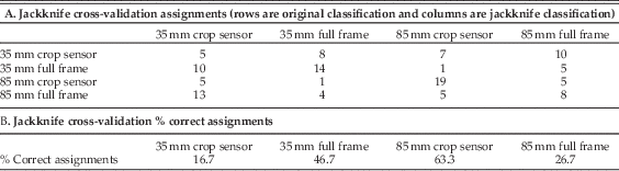
Figure 8 presents the results of the zoom experiment. The variation between full frame and crop sensor exerts a systematic effect along PC2; there is also some systematic variation with zoom. Higher zooms (e.g., 70–85 mm) generally plot within the 95% confidence ellipses, suggesting that these photographs are the least distorted and most representative of the true shape of the specimens.
PCA plot of the “zoom experiment”; zoom in millimeters is labeled for each point. Images taken using the crop sensor are separable from those taken with a full frame. The 95% confidence ellipses are shown. See Table 1 for photographic setup. PC1 and PC2 account for 41% of the total variance in the data set (PC1=26%, PC2=15%)

Data Accessibility
Image data sets (both the full data set and the “zoom experiment”) and associated .tps files of digitized coordinates, and the Procrustes-superimposed coordinates for the data sets, are available in the Supplemental Material on Dryad.
Discussion
In many applications of morphometrics, it is probable that the natural variation within a set of specimens of a species will be larger than the bias that may be introduced by photographic methods if data are collected using a consistent method and setup. However, in some situations, photographic distortion will be significant and nonuniform within the data set, as specimens that vary in size or coplanarity of landmarks (i.e., varying degrees of concavity or convexity) may require different camera settings to be used (e.g., zoom, f-stop, exposure), or photographs may be collected over a period of time or using different lenses and/or cameras. Equally, sometimes researchers may not be able travel to collections to photograph specimens themselves, and institutions may have in-house policies about “standard” photographic setups they use for images supplied on request, and it is likely that these in-house policies will vary between institutions. In these situations, care should be taken by researchers to minimize, or at least quantify, the inherent variation in the data sets they collect. We accept that there are (probably many) situations in which the use of different photographic setups is unavoidable; and while we have shown that different photographic methods can introduce statistically significant effects on the recovery of “true” shape, we have also demonstrated that these effects can be corrected for.
We have also demonstrated that if photographic bias not corrected for, naïve use of commonly applied analyses such as CVA and ANOVA can give misleading results. The results of the CVA suggest strongly that if subsets of specimens of a data set composed of a single or a number of closely related species were photographed using different cameras and/or photographic methods, the variation introduced simply by differences in methods could cause investigators to recognize groupings of specimens with no biological foundation. This would occur, for instance, if specimens assigned to some taxon or other group of interest were held by a single institution and a researcher requested or was only permitted photographs taken in-house by the institution, rather than specimen loans.
Distortion of images is greatest at the edges of the frame, regardless of the type of distortion. Since their release, the most prevalent digital SLR cameras have been crop sensor, because full-frame sensors were expensive, which meant that, by default, the edges of the field of view where the distortion was greatest were excluded from the photograph. With the advent of more affordable full-frame digital SLR cameras, the edges of the field of view that were previously excluded from the photograph are now being incorporated. If care is not taken to modify photographic practices accordingly, workers today may introduce significantly greater amounts of distortion into their data sets than previously. In general, the wider the angle of the lens that is used, the more distortion there will be. Accordingly, it is not necessarily preferable to use a wide-angle lens that allows for the camera to be close to the specimen, as such a lens would likely result in more distortion than use of a lens with greater zoom that requires the camera to be farther away from the specimen. This is logical when one considers the types of photographs that are taken by a fish-eye lens (e.g., 10–20 mm), which have a very wide field of view but a lot of distortion.
The crop sensor does not have the same field of view as the full-frame image sensor, and thus “trims” the edges off the field of view that is available to the full-frame sensor. So if the specimen is within the field of view of the crop sensor, no part of the specimen will be near the edge of the full-frame sensor field of view, where distortion is greatest. This should mean that images taken with a crop-sensor camera (or one using a crop-sensor setting) will be less distorted overall and will require less digital processing to correct any residual distortion. Figure 8 shows that the raw images taken with the crop-sensor setting reflect this—they cluster more tightly than those taken with the full-frame setting, and there are fewer outliers.
The exact setup a researcher chooses to use will depend entirely on what kind of specimens he or she is photographing. Obviously, a gridded background cannot usefully be incorporated in photographs of specimens still embedded in slabs (e.g., the trilobite cephala illustrated in Webster and Sheets Reference Webster and Sheets2010), and a 5 mm grid such as we have used here would not be appropriate for a cetacean skull data set (e.g., Tsai and Fordyce Reference Tsai and Fordyce2014). Placement of the specimen and the scale bar as close to the center of the field of view as practicable is vital, and the logistics of doing so will vary from data set to data set and specimen to specimen.
Fortunately, the simple step of using an initial photo of a sheet of grid paper to establish a lens correction in a photographic computer program such as Adobe Photoshop for every photo taken with the same camera settings will minimize the variance incorporated into morphometric experiments by photographic distortion.
Recommendations
Distortion is inherent in photography, and it should not be ignored as part of a morphometric workflow. The more morphologically similar the taxa of interest are, the more influence photographic distortion will exert on the data set, and this is a source of error that should be taken into account, in the same manner as one would account for operator error introduced by the person doing the data capture during digitization of landmarks from photographs (Webster and Sheets Reference Webster and Sheets2010).
This study has considered the distortion that can be introduced using one camera and one lens to photograph a specific group of organisms—bivalve mollusks. Every data set and every camera and lens will vary, and the effect of distortion unique to the data set and setup being used should be assessed to ensure that it is not a significant source of error in any given morphometric study. A number of recommendations can be drawn from this study to minimize and quantify the effect of photographic distortion on a data set. The key points can be summarized as follows:
-
∙ Avoid mixing data sets from different cameras, different lenses, and/or different photographic setups.
-
∙ Distortion is greatest at the margins of the photograph, so avoid placing the specimen and the scale bar there if at all possible.
-
∙ Maintain constant camera settings (insofar as is practical) throughout the photographing of a set of specimens (i.e., f-stop, zoom, shutter speed) to minimize the variation in how these factors are distorting the photographs.
-
∙ Be aware that full-frame cameras will likely distort photographs more than crop-sensor cameras, as they have a wider field of view and will have more distortion near the edges of the photograph.
-
∙ Use a reference grid (either included within each photograph, if possible, or as the first photograph taken with each new camera setup) to quantify and correct for distortion induced by each camera in a study.
Acknowledgments
We are grateful to Martin and Jill Higgins for collecting the mactrid specimens used in this study. We would like to thank Guillaume Duclaux and James Crampton for their reviews of early drafts of this paper, Russell Bicknell for his statistical advice, and Roma Klapaukh for his help with R code. We also thank J. W. Huntley and an anonymous reviewer for their thoughtful and helpful reviews of the manuscript.
Supplementary materials
Data available from the Dryad Digital Repository: http://dx.doi.org/10.5061/dryad.ht288