1. Introduction
The quantitative description of electro–kinetic (EK) phenomena at charged interfaces began in 1903, when Smoluchowski (Smoluchowski Reference Smoluchowski1903) derived expressions for electro–osmotic flow and streaming current by applying the Stokes equation of hydrodynamics within electric double layers (EDLs) – remarkably, without any knowledge of the equilibrium potential or ion distributions. Since then, EK phenomena and other coupled transport processes originating in EDLs have become of major importance in numerous applications. Examples include the control of fluid motion and particle manipulation in microfluidic systems (Stone et al. Reference Stone, Stroock and Ajdari2004), membrane-based processes for water desalination and filtration (Jones et al. Reference Jones, Qadir, van Vliet, Smakhtin and Kang2019), energy storage devices such as lithium-ion batteries and supercapacitors (Grey & Hall Reference Grey and Hall2024), emerging technologies for harvesting osmotic energy from salinity gradients (Chapuis & Bocquet Reference Chapuis and Bocquet2025), nanofluidic devices for single-molecule sensing and separation (Bocquet Reference Bocquet2020; Gonella et al. Reference Gonella2021) and others. In all these systems, the coupled transport of ions, charge and solvent in the presence of EDLs determines both performance and efficiency. However, the theoretical foundations underlying these technological advances remain insufficiently tested, leading to persistent discrepancies among different experimental approaches (Lyklema Reference Lyklema1994).
While the equilibrium properties of electrostatic double layers are now considered well-described both theoretically and experimentally, this is not the case for their dynamic counterparts. A decade after Smoluchowski’s work, Gouy and Chapman independently developed the equilibrium theory of EDLs by solving the Poisson–Boltzmann equation in the presence of charged interfaces. This Gouy–Chapman theory became the foundation for understanding electrostatic interactions in electrolytes, and was experimentally validated in the late 1970s using the surface force apparatus (SFA) (Tabor & Winterton Reference Tabor and Winterton1969; Israelachvili & Adams Reference Israelachvili and Adams1978; Horn et al. Reference Horn, Smith and Haller1989; Israelachvili Reference Israelachvili2011). Measurements confirmed that the Gouy–Chapman theory accurately describes the diffuse layer beyond a few nanometres from dielectric surfaces, in dilute solutions of monovalent electrolytes (typically below 0.1 M, i.e. for Debye length larger than the ion size) (Horn et al. Reference Horn, Smith and Haller1989).
Regarding the dynamic behaviour of EDLs, Smoluchowski’s expression for electrophoretic velocity is widely used to determine the zeta potential, which corresponds to the electrostatic potential at the plane of zero velocity. Following Smoluchowski’s pioneering work, the theory of diffusio–EK interfacial transport – coupling the fluxes of electrical charges, solute and the flow rate – was derived by applying the Stokes equation within EDLs assumed to be at equilibrium in the direction normal to the surface (Gross & Osterle Reference Gross and Osterle1968; Prieve et al. Reference Prieve, Anderson, Ebel and Lowell1984). However, the dynamic behaviour of EDLs under flow conditions remains insufficiently tested experimentally. For example, the surface charge deduced from the zeta potential using the equilibrium Grahame relation (Grahame Reference Grahame1953) is rarely compared with the value obtained from direct force measurements within the Derjaguin–Landau–Verwey–Overbeek (DLVO) framework. Moreover, surface charge values obtained from zeta potential measurements often differ by several orders of magnitude from those derived from EDLs electrical conductance, even though both determinations rely on the same classical theoretical framework (Lyklema Reference Lyklema1994; Bonthuis & Netz Reference Bonthuis and Netz2012; Siria et al. Reference Siria, Poncharal, Biance, Fulcrand, Blase, Purcell and Bocquet2013; Hartkamp et al. Reference Hartkamp, Biance, Fu, Dufrêche, Bonhomme and Joly2018). Netz and coworkers proposed that spatial variations in viscosity and dielectric constant profiles could explain these discrepancies (Bonthuis & Netz Reference Bonthuis and Netz2012), but this interpretation requires further experimental testing. Despite advances in measurement sensitivity, direct experimental validation of classical diffusio–EK theory remains lacking.
Dynamic SFA (D-SFA) and colloidal probe atomic force microscope (CP-AFM), which have demonstrated the ability to measure both equilibrium DLVO forces and dynamic viscous forces (Cottin-Bizonne et al. Reference Cottin-Bizonne, Cross, Steinberger and Charlaix2005; Maali et al. Reference Maali, Cohen-Bouhacina and Kellay2008; Garcia et al. Reference Garcia, Barraud, Picard, Giraud, Charlaix and Cross2016; Lizée et al. Reference Lizée, Coquinot, Mariette, Siria and Bocquet2024), offer promising experimental platforms for validating EK theory. Liu et al. (Reference Liu, Klaassen, Zhao, Mugele and van den Ende2018) used a dynamic AFM to measure the real and imaginary part of the electroviscous force involved in squeezing out thin films of aqueous electrolyte between an AFM tip and silica substrates. Rodríguez Matus et al. (Reference Rodríguez Matus, Zhang, Benrahla, Majee, Maali and Würger2022) used a CP-AFM to investigate the viscoelastic response of a confined electrolyte film in a sphere–plane geometry. Both works reported that the measured damping force is significantly enhanced as compared with the pure Reynolds lubrication force (hereafter called the Reynolds force), when the gap between the surfaces becomes of the order of the Debye length, or below. Theoretical models, although they capture the qualitative trends observed in these experiments, do not provide a correct quantitative description of the data. Overall, existing theoretical models remain insufficient for comprehensive experimental validation, as they have not described the electrohydrodynamic forces during the drainage of thin electrolyte films in these geometries across all relevant parameters and degrees of EDLs overlap.
To be more precise, several authors have investigated hydrodynamic forces during drainage in the sphere–plane geometry, predicting electroviscous effects of various kinds. Hinch and Sherwood (Hinch & Sherwood Reference Hinch and Sherwood1983) analysed the primary electroviscous effect in suspensions when the Debye length is small compared with the particle radius. They identified scaling regimes that depend on the electric Hartmann number
 $\textit{Ha}$
– which characterises the ratio of electric to viscous stress in the fluid – and on the surface potential, with non-monotonic behaviour at high charge. Cox (Cox Reference Cox1997) extended this analysis to more general geometries, in the limit of very thin EDLs, using systematic matched asymptotic expansions. van de Ven and coworkers (van de Ven et al. Reference van de Ven, Warszynski and Dukhin1993) reported attractive electroviscous forces between spheres moving parallel to each other in opposite directions, arising from Maxwell stress contributions. Yariv and coworkers (Yariv et al. Reference Yariv, Schnitzer and Frankel2011; Schnitzer et al. Reference Schnitzer, Frankel and Yariv2012) identified the scaling
 $\textit{Ha}=(\alpha /\textit{Pe}) \delta ^{-2}$
between the Hartmann
 $\textit{Ha}$
and Péclet
 $\textit{Pe}$
numbers in the thin-double-layer limit, where
 $\alpha$
is the dimensionless electric field at the surfaces and
 $\delta$
is the ratio of the Debye length to a characteristic length scale. They derived macroscale models with effective boundary conditions for tangential motion in both large-Péclet (Part 1) and moderate-Péclet (Part 2) regimes.
In the specific context of normal drainage flows, Bike and Prieve (Bike & Prieve Reference Bike and Prieve1990) calculated corrections to the Reynolds force at separations much larger than the Debye length, later extended by Würger and coworkers (Rodríguez Matus et al. Reference Rodríguez Matus, Zhang, Benrahla, Majee, Maali and Würger2022). However, these models lack analytical expressions outside asymptotic regimes and entirely neglect the transport of solute. More recently, Mugele and coworkers (Liu et al. Reference Liu, Klaassen, Zhao, Mugele and van den Ende2018; Zhao et al. Reference Zhao, Zhang, van den Ende and Mugele2020) developed a diffusion-dominated model applicable to small AFM tips where convection is negligible, but unsuitable for D-SFA and larger CP-AFM probes.
In this paper, we present a semianalytical theory for normal hydrodynamic forces during the drainage of thin electrolyte films between dielectric surfaces, applicable to D-SFA and CP-AFM experiments in the linear response regime. Our model derives a local Onsager formalism for the coupled transport of fluid, charge and solute, integrated across the film thickness. It requires a small gap and local equilibrium across thickness, but imposes no limitation on the radial Péclet number. The model addresses all stages of EDLs overlap connecting to the equilibrium phase diagram (Andelman Reference Andelman2006; Adar & Andelman Reference Adar and Andelman2018), and can be adapted to various electrical, chemical or hydrodynamic boundary conditions. We explore in detail the case of a monovalent electrolyte with constant surface charge and no-slip boundary conditions.
In addition to the pure lubrication force, we identify and quantify two distinct contributions to the so-called electroviscous force: (i) an EK damping force proportional to the driving rate, resulting from the streaming current and compensating electric field; and (ii) a diffusio–kinetic (DK) force generated by concentration gradients and diffusio–osmotic flows. We derive scaling laws for these contributions across all separation regimes – from non-overlapping EDLs at high and low Dukhin numbers, to overlapping EDLs within the Gouy–Chapman, Debye–Hückel and ideal-gas (or Donnan) approximations. Our results predict measurable signatures, including non-monotonic variation of the damping with the surface charge, apparent hydrodynamic stagnant layers, and a long-range algebraic decay of the DK stiffness – all accessible to experimental verification through combined equilibrium and dynamic measurements without fitting parameters.
2. Electrohydrodynamic forces in the sphere–plane geometry: the Derjaguin approximation
2.1. General framework of the model
Our model describes applications such as D-SFA or CP-AFM. We consider two solid spheres of the same radius
 $2R$
, physically identical to each other, separated by a small distance
 $D\ll R$
. In the framework of the Derjaguin approximation (Israelachvili Reference Israelachvili2011) and the related approximations developed below, this geometry is equivalent to a sphere of radius
 $R$
and a plane. We assume a full symmetry around the axis
 $Oz$
defined by the sphere centres, with the origin
 $O$
(a fixed point) located midway between the two spheres, and a plane symmetry across
 $z=0$
. The cylindrical coordinates are denoted as
 $(O,r,z)$
, the gap between the surfaces at the radial distance
 $r$
is
 $h(r,t)$
. The system defined in this manner is depicted in figure 1. A list of the main variables used in the paper is provided in Appendix A.
The solids are immersed in a solution of monovalent electrolyte with bulk number density
 $n_0$
(number of cations and anions per unit volume). The solids are assumed to be dielectric and their surface bears a surface charge
 $\sigma$
. The relative velocity of the spheres is denoted as
 $\dot D$
. In §§ 4 and 6 we will focus on the case of a harmonic driving at angular frequency
 $\omega$
and small amplitude
 $h_0$
around a fixed distance
 $D$
, corresponding to a relative sphere velocity
 $\dot D=h_0\omega \text{Re} [e^{i\omega t}]$
.
The quantity of interest is the force
 $F$
acting on the upper sphere along the
 $Oz$
axis of symmetry. We consider only contributions to the force arising from electrostatics in the mean-field approximation, hydrodynamics and electrokinetics. We refer to § 7 for a discussion of other effects and range of validity of our model.
Schematics of the system geometry: an electrolytic solution is confined between two identical spheres of curvature radius
 $2R$
and whose separation
 $D(t)$
varies in time.

Our model uses the standard formulation of the EK theory in the regime of slowly varying fields, i.e. it neglects the magnetic field and wave propagation. The transport of ions is governed by the Nernst–Planck equation. The number density of cations and anions is denoted as
 $n^+$
and
 $n^-$
, their diffusion coefficient
 $D^+$
and
 $D^-$
, their electrochemical potential
 $\mu ^+=k_{\textit{B}}T \ln (n^+/n_0)+eV$
and
 $\mu ^-=k_{\textit{B}}T \ln (n^-/n_0)-eV$
, where
 $T$
is the temperature,
 $k_{\textit{B}}$
the Boltzmann constant,
 $V$
the electric potential and
 $e$
the elementary charge.
In D-SFA (
 $R\sim 3\,\textrm {mm}$
) and CP-AFM (
 $R\sim 10$
 ${\unicode[Arial]{x03BC}}$
m) experiments, the Reynolds number is usually very low. An upper limit is
 $\textrm{Re} \leq \rho \textit{v}_r D/\eta$
with
 $\rho$
the liquid density,
 $\eta$
the liquid viscosity and
 $\textit{v}_r= \dot D\sqrt {R/D}$
a maximum radial velocity. The driving rate in local probe measurements is usually at most
 $\dot D/D \lt 0.1\,$
s
 $^{-1}$
, and the working distance
 $D \lt R/100$
. With the density and viscosity of water, the Reynolds number does not exceed
 $10^{-3}$
. The flow will thus be described by the incompressible Stokes equation. We introduce the hydrodynamic stress tensor and the electrostatic Maxwell stress tensor:
 \begin{eqnarray} \unicode{x1D64E}^{\mathcal H} = -P\unicode{x1D644} + \frac {\eta }{2} ({\boldsymbol{\nabla }}\boldsymbol{v}+^t{\boldsymbol{\nabla }} \boldsymbol{v}) \quad \vert z \vert \lt h/2 , \end{eqnarray}
 \begin{eqnarray} \unicode{x1D64E}^{\mathcal M} = \varepsilon _i\left ({-}\frac {\Vert \boldsymbol{\nabla } V \Vert ^2}{2}\unicode{x1D644}+\boldsymbol{\nabla } V \otimes \boldsymbol{\nabla } V \right ) \quad \begin{cases} \varepsilon _i=\varepsilon _{\textit{l}} \ \ \textrm {if} \ \vert z \vert \lt h/2,\\ \varepsilon _i=\varepsilon _{\textit{s}} \ \ \textrm {if} \ \vert z \vert \gt h/2, \end{cases} \end{eqnarray}
where
 $\boldsymbol{v}=\textit{v}_r \boldsymbol{e}_r+\textit{v}_z\boldsymbol{e}_z$
is the flow velocity,
 $\unicode{x1D644}$
the identity matrix,
 $P$
the pressure in excess of the atmospheric pressure,
 $\eta$
the liquid viscosity which will be assumed independent of the ion concentrations and
 $\varepsilon _{\textit{l}}$
,
 $\varepsilon _{\textit{s}}$
the dielectric permittivities of the liquid and of the solids, respectively. With these notations, the Poisson, Nernst–Planck and Stokes equations, as well as the conservation laws for the ions and the incompressible fluid, are
 \begin{align} \boldsymbol{\nabla} ^2 V = - \frac {e (n^+-n^-)}{\varepsilon _{\textit{l}}} \quad \vert z \vert \lt h/2 \quad \boldsymbol{\nabla} ^2 V =0 \quad \vert z \vert \gt h/2 , \end{align}
 \begin{align} \boldsymbol{j}^{\pm }=-\frac {D^{\pm }}{k_{\textit{B}}T} n^{\pm } \boldsymbol{\nabla } \mu ^{\pm } + n^{\pm } \boldsymbol{v} , \end{align}
 \begin{align} \textrm {div} (\unicode{x1D64E} ^{\mathcal M}+\unicode{x1D64E} ^{\mathcal H}) = \boldsymbol{0} = -\boldsymbol{\nabla }\! P + \eta \boldsymbol{\nabla} ^2 \boldsymbol{v} - e (n^+-n^-) \boldsymbol{\nabla } V , \end{align}
 \begin{align} \frac {\partial n^{\pm }}{\partial t} =-\textrm {div} \boldsymbol{j}^{\pm } \quad \textrm {div} \boldsymbol{v} = 0 . \end{align}
The boundary conditions at the symmetry plane
 $z=0$
(quantities at
 $z=0$
are hereafter denoted with the subscript m), correspond to invariance by the transformation
 $z \rightarrow -z$
:
 \begin{equation} z=0, \quad \textit{v}_{z,\textit{m}}=0 , \quad \frac {\partial V}{\partial z}\bigg |_{\textit{m}}=0 , \quad \frac {\partial \mu ^{\pm }}{\partial z}\bigg |_{\textit{m}}=0 , \quad \frac {\partial \textit{v}_r}{\partial z}\bigg |_{\textit{m}} = 0 . \end{equation}
At the liquid–solid interface
 $z=h/2$
we will use the continuity of the electric potential and the Maxwell–Gauss equation for the normal component of the electrical displacement. We will also assume a no-slip boundary condition. Quantities at
 $z=h/2$
are denoted with the subscript
 $w$
and satisfy
 \begin{align} V_{{w}^-}=V_{{w}^+}, \end{align}
 \begin{align} - \varepsilon _{\textit{s}} \boldsymbol{\nabla } V \vert _{{w}^+} \boldsymbol{\cdot }\boldsymbol{n} + \varepsilon _{\textit{l}} \boldsymbol{\nabla } V \vert _{{w}^-}\boldsymbol{\cdot }\boldsymbol{n}= \sigma ,\end{align}
 \begin{align} \boldsymbol{v}_{{w}}= \frac {\dot D}{2} \boldsymbol{e}_z,\end{align}
 \begin{align} (\boldsymbol{j}^{\pm }_{{w}}-n^{\pm } \boldsymbol{v}_{{w}})\boldsymbol{\cdot }\boldsymbol{n}=j^{\pm ,\textit{source}}. \end{align}
Here
 $\boldsymbol{n}$
denotes the unit normal to the upper sphere surface, pointing from the liquid into the upper sphere. The superscripts
 ${w}^-$
and
 ${w}^+$
refer, respectively, to the liquid and solid sides of the interface. The source terms
 $j^{\pm ,\textit{source}}$
account for the charge regulation phenomena at a dielectric surface when the surface charge is not fixed, and describe the associated adsorption/emission of ions.
Without loss of generality, we take
 $\sigma \gt 0$
in the following. We also consider that
 $V(r=\infty )=0$
, i.e. no electric field applied in the reservoir.
The total stress is continuous through the interface. We denote
 $\boldsymbol{F}$
the force that an external operator has to apply in order to maintain the prescribed driving velocity
 $\dot {D}$
of the upper sphere, and
 $F=\boldsymbol{F} \boldsymbol{\cdot }\boldsymbol{e}_z$
its component on the
 $z$
-axis. The force balance on the upper sphere projected on the
 $z$
-axis gives
 \begin{equation} F = \boldsymbol{e}_z \boldsymbol{\cdot }\left ( \oint _{S} \left (\boldsymbol{S}^\mathcal{H} + \boldsymbol{S}^\mathcal{M}\right )\big |_{{w}^-} \boldsymbol{\cdot }({-}\boldsymbol{n}) \,\mathrm{d}S -\oint _{S} \boldsymbol{S}^\mathcal{M}\big |_{{w}^+} \boldsymbol{\cdot }({-}\boldsymbol{n}) \,\mathrm{d}S \right ) \end{equation}
where
 $\boldsymbol{n}$
is the unit normal defined above (pointing from the liquid into the upper sphere). The first integral is the traction exerted by the liquid on the sphere and the second the traction exerted by the Maxwell stress in the dielectric solid.
Our model calculates the force response within two further approximations:
-
(i) the Derjaguin approximation (Israelachvili Reference Israelachvili2011) and its consequences discussed in the next subsection;
-
(ii) the approximation of local thermodynamic equilibrium (LTE) across the thickness
 $h$
of the liquid film, developed in § 3.

2.2. The Derjaguin approximation
The Derjaguin approximation assumes that the interacting surfaces are nearly parallel. Therefore, the unit normal vector to the surfaces in the interaction region is well approximated by the axial direction:
 $\boldsymbol{n} \approx \boldsymbol{e}_z$
. While the condition for the approximation is well established and widely used for equilibrium interactions, its application to electrohydrodynamic interactions requires more careful consideration.
Equilibrium interactions. For electrostatic interactions in an electrolyte, the characteristic decay length is the Debye length
 $\ell _{\textit{D}}$
. In the sphere–plane geometry with minimal gap
 $D$
, electrostatic interactions become negligible when the local gap exceeds a few Debye lengths. Using the parabolic approximation for the gap,
 \begin{equation} h (r, t) = D(t) + \frac {r^2}{2R} \end{equation}
the lateral extent of the electrostatic interaction region is
 $r \sim \sqrt {R\ell _{\textit{D}}}$
. The maximum slope of the surfaces over this lateral distance is
 \begin{equation} \left |\frac {\textrm{d}h}{\textrm{d}r}\right |_{r \sim \sqrt {R\ell _{\textit{D}}}} \sim \frac {\sqrt {R\ell _{\textit{D}}}}{R} = \sqrt {\frac {\ell _{\textit{D}}}{R}} \ll 1 .\end{equation}
Hydrodynamic interactions. The hypothesis of nearly parallel surfaces corresponds to the condition for the lubrication approximation of the Stokes equation. There is no intrinsic characteristic decay length for the hydrodynamic interaction as the pressure field in a lubrication flow between curved surfaces decays algebraically with the separation distance
 $D$
. However, Brenner (Reference Brenner1961) showed that the hydrodynamic pressure becomes negligible beyond a lateral distance of order
 $\sqrt {RD}$
from the apex. This defines the lateral extent of the hydrodynamic interaction region. The maximal slope of the surfaces at this lateral distance is
 \begin{equation} \left |\frac {\textrm{d}h}{\textrm{d}r}\right |_{r \sim \sqrt {RD}} \sim \frac {\sqrt {RD}}{R} = \sqrt {\frac {D}{R}} \ll 1 .\end{equation}
Physical consequences. Defining
 $\lambda = \max (\ell _{\textit{D}}, D)$
as the maximum interaction range in the normal direction, the condition
 $\lambda \ll R$
ensures a separation of length scales between normal variations (over scale
 $\sim \lambda$
) and lateral variations (over scale
 $\sim \sqrt {R\lambda }$
). For any quantity
 $a$
that varies significantly across the film thickness the following inequality holds:
 \begin{equation} \left \vert \frac {\partial a}{\partial r} \right \vert \ll \left \vert \frac {\partial a}{\partial z} \right \vert \quad \vert z \vert \le \frac {h}{2} .\end{equation}
An important consequence is that the Poisson equation in the liquid ((2.3a
),
 $\vert z \vert \lt h/2$
) and its boundary condition (2.5b
) reduce to their one-dimensional form:
 \begin{equation} \frac {\partial ^2 V}{\partial z^2} = -\frac {e (n^+-n^-)}{\varepsilon _{\textit{l}}} \quad \left .\frac {\partial V}{\partial z}\right \vert _{{w}^-} = \frac {\sigma }{\varepsilon _{\textit{l}}} .\end{equation}
It is shown in Appendix B that the normal electric field in the dielectric solids is of the same order as the radial field
 $(\partial V/\partial r) (h^-/2)$
, which is negligible according to inequality (2.10). By integrating equation (2.11) along
 $z$
the local electroneutrality condition is obtained:
 \begin{equation} \int _0^{h (r,t) /2}e (n^+-n^-) (r,z,t) \textrm {d}z=-\sigma .\end{equation}
With
 $\boldsymbol{n} \approx \boldsymbol{e}_z$
and inequality (2.10), the force per unit surface due to the Maxwell stress tensor at the interface is
 \begin{align} \unicode{x1D64E}^{\mathcal M}_{{w}} \boldsymbol{n} \approx S^{\mathcal M}_{zz} \boldsymbol{e}_z \approx \frac {\varepsilon _i}{2}\left (\frac {\partial V}{\partial z} \right ) ^2 \boldsymbol{e}_z .\end{align}
This contribution is negligible in the dielectric solids (see Appendix B). With
 $\boldsymbol{n}\approx \boldsymbol{e}_z$
and
 $\mathrm{d}S \approx 2\pi r\,\mathrm{d}r$
, the force (2.6) reduces to
 \begin{align} F & = - \int _0^{\infty }2\pi r (S ^{\mathcal M}_{zz}+S ^{\mathcal H}_{zz}) (r,h^-/2) \textrm {d}r \nonumber \\ &= - \int _0^{\infty }2\pi r \left [-P+\eta \frac {\partial \textit{v}_z}{\partial z} +\frac {\varepsilon _{\textit{l}}}{2}\left (\frac {\partial V}{\partial z} \right ) ^2 \right ] \left (r,\frac {h^-}{2}\right ) \textrm {d}r. \end{align}
We show in Appendix B that within our approximations the quantity in brackets is uniform across the film thickness and that the force reduces to
 \begin{equation} F=\int _0^\infty 2\pi r P (r,0) \textrm {d}r .\end{equation}
3. Approximation of local equilibrium across the film thickness
3.1. Conditions for time scale separation
In addition to the separation of length scales
 $h_0\ll D \ll R$
, we assume that the diffusion time
 $\tau _z$
across the thickness of the electrolyte film is much shorter than the time scale of the driving:
 \begin{equation} \tau _z = \frac {D^2}{D^\pm } \ll \tau =\frac {D}{\dot D} \quad \textrm {or} \quad \tau =\frac {2\pi }{\omega } .\end{equation}
For a continuous-like driving at velocity
 $\dot D$
, the time scale separation is equivalent to the condition of small normal Péclet number. For an oscillatory driving at amplitude
 $h_0\ll D$
, the small-normal-Péclet condition is not sufficient and the time scale separation requires a condition on the driving frequency.
In these conditions of spatial and time scales separations the transport equation (2.3d
) reduces to
 $\partial _z\! (n^{\pm }\partial _z \mu ^{\pm } )=0$
to the leading order in
 $\tau _z/\tau$
(see also Appendix B.3). Together with the boundary condition at
 $z=0$
this gives
 $\partial \mu ^{\pm }/\partial z=0$
to the leading order in
 $\tau _z/\tau$
, which is the approximation of LTE:
 $\mu ^{\pm }$
are uniform across the film thickness. This relies only on the midplane symmetry (2.4) and not on the condition at the walls: the possible ion source in (2.5d
) feeds only the thickness-integrated balances, so the result holds whether or not surface sources are present.
The range of driving rate, or driving frequency, for the time scale separation depends on the working range
 $D$
and on the diffusion coefficient of ions. Taking the case of a KCl electrolyte of average diffusion coefficient 2.0
 $\times 10^{-9}\textrm {m}^2$
s−1 in water at 300 K (Haynes Reference Haynes2016), typical values are as follows.
The D-SFA. With a typical working distance
 $D\lesssim 1\,$
µm (Garcia et al. Reference Garcia, Barraud, Picard, Giraud, Charlaix and Cross2016), the characteristic time is
 $\tau _z\lesssim 10^{-3}\,\textrm {s}$
. For working frequencies typically spanning between
 $5\,\textrm {Hz}$
and
 $500\,\textrm {Hz}$
, the condition
 $\tau _z \ll 2\pi /\omega$
is well satisfied.
The CP-AFM. With a working distance
 $D\lesssim 100\,\textrm {nm}$
(Liu et al. Reference Liu, Klaassen, Zhao, Mugele and van den Ende2018; Rodríguez Matus et al. Reference Rodríguez Matus, Zhang, Benrahla, Majee, Maali and Würger2022) the characteristic time is
 $\tau _z\lesssim 10^{-5}\,\textrm {s}$
. The hypothesis of local equilibrium across the film is appropriate for driving rates or working frequencies up to
 ${\sim} 100\,\textrm {kHz}$
.
3.2. Thermodynamic potentials
We introduce the nominal Debye length
 $\ell _{\textit{D}}$
associated with the electrolyte concentration
 $n_0$
in the reservoir, the nominal Gouy length
 $\ell _{\textit{G}}$
associated with the surface charge
 $\sigma _0$
of non-interacting surfaces at rest, the Bjerrum length
 $\ell _{\textit{B}}$
, and the dimensionless parameter
 $\alpha$
(Saville Reference Saville1977; Israelachvili Reference Israelachvili2011; Adar & Andelman Reference Adar and Andelman2018):
 \begin{equation} \ell _{\textit{B}}=\frac {e^2}{4\pi \varepsilon _{\textit{l}} k_{\textit{B}}T}, \quad \ell _{\textit{D}}=\sqrt {\frac {\varepsilon _{\textit{l}} k_{\textit{B}} T}{2e^2 n_0}}=\sqrt {\frac {1}{8\pi \ell _{\textit{B}} n_0}}, \quad \frac {2}{\ell _{\textit{G}}}=\frac {\sigma _0 e}{\varepsilon _{\textit{l}} k_{\textit{B}}T}, \quad \alpha =\frac {2\ell _{\textit{D}}}{\ell _{\textit{G}}} .\end{equation}
In order to decouple electrical from chemical effects in the transport equations, sum and difference potentials are introduced as
 \begin{equation} \mu _{\textit{s}}=\frac {\mu ^++\mu ^-}{2}=k_{\textit{B}}T\ln \frac {n (r,t)}{n_0}, \quad W=\frac {\mu ^+-\mu ^-}{2e}, \quad \chi (r,z,t) =\frac {e (V-W)}{k_{\textit{B}}T} .\end{equation}
The average chemical potential
 $\mu _{\textit{s}}$
and electrical potential
 $W$
are uniform along
 $z$
. The quantity
 $n (r,t) =n_0 e^{\mu _{\textit{s}}/k_{\textit{B}}T}$
is the equivalent bulk concentration at position
 $r$
and time
 $t$
. Using
 $n^{\pm }=n_0\exp [(\mu ^{\pm }\mp eV)/k_{\textit{B}}T]$
the sum and difference ion densities are derived:
 \begin{equation} n_{\textit{s}}=n^++n^-=2n (r,t) \cosh \chi, \quad n_{\textit{e}}=n^+-n^-=-2n (r,t) \sinh \chi. \end{equation}
The Poisson equation (2.3a ) and its boundary condition (2.5a ) become
 \begin{align} \frac {\partial ^2\chi }{\partial z^2}=\frac {\sinh \chi }{\lambda _{\textit{D}}^2}, \quad \lambda _{\textit{D}} = \sqrt {\frac {\varepsilon _{\textit{l}} k_{\textit{B}} T}{2e^2 n(r,t)}}=\sqrt {\frac {n_0}{n(r,t)}}\ell _{\textit{D}}, \end{align}
 \begin{align} \left .\frac {\partial \chi }{\partial z}\right \vert _{h/2(r,t)}= \frac {2}{\lambda _{\textit{G}}}, \quad \frac {2}{\lambda _{\textit{G}}}=\frac {\sigma (r,t) e}{\varepsilon _{\textit{l}} k_{\textit{B}}T} .\end{align}
Thus,
 $\chi (z)$
satisfies a Poisson–Boltzmann equation along
 $z$
with local parameters. The analytical solution
 $\chi$
of (3.5a
) for a positive surface charge is (Ninham & Parsegian Reference Ninham and Parsegian1971)
 \begin{align} \chi (r,z,t) =\chi _{\textit{m}} (r,t) -\ln [\textrm {cd}(z/2 \lambda _{\textit{D}} \sqrt {k} \vert k^2) ]^2 \quad k (r,t) =e^{-\chi _{\textit{m}} (r,t)}, \end{align}
 \begin{align} \cosh \chi _{{w}} (r,t) -\cosh \chi _{\textit{m}} (r,t)= \frac {2 \lambda _{\textit{D}}^2}{\lambda _{\textit{G}}^2}= \frac {\alpha ^2}{2}\frac {n_0}{n(r,t)} \frac {\sigma (r,t)^2}{\sigma _0^2}, \end{align}
where
 $\textrm {cd} (u \vert k^2)$
is the Jacobi elliptical function of argument
 $u$
and parameter
 $k^2$
, and
 $k(h,n,\sigma )$
is determined by the boundary condition (3.5b
) (see Appendix D).
At a large distance from the sphere–plane axis the EDLs do not overlap, the midplane potential vanishes, and
 $k=1$
. In the following we denote
 $\psi =\chi _{\textit{eq}}$
the equilibrium potential
 $\chi$
when the surfaces are not moving (
 $n\equiv n_0$
everywhere). In our hydrodynamic condition of no-slip at the solid surfaces, the equilibrium surface potential of a non-interacting surface reduces to its nominal zeta potential, and satisfies the Grahame (Reference Grahame1953) equation:
 \begin{equation} \tilde \zeta = \frac {e\zeta }{k_{\textit{B}}T}=\psi _{w,\textit{0}}, \quad \cosh \tilde \zeta = \frac {\alpha ^2}{2}+1, \quad \sinh \frac {\tilde \zeta }{2}=\frac {\alpha }{2}. \end{equation}
3.3. Transport equations
The transport equations are written in terms of the sum and difference variables by introducing the average diffusion coefficient and the diffusion coefficient contrast:
 \begin{equation} D_{\textit{s}}=\frac {D^++D^-}{2}, \quad \delta = \frac {D^+-D^-}{D^++D^-}, \quad D^{\pm }=D_{\textit{s}} (1\pm \delta ). \end{equation}
Similarly we define the sum and difference number flow densities as
 \begin{equation} \boldsymbol{j}_{\!\textit{s}}=\boldsymbol{j}^++\boldsymbol{j}^- ,\quad \boldsymbol{j}_{\!\textit{e}}=\boldsymbol{j}^+-\boldsymbol{j}^- .\end{equation}
Using (3.3) and (3.4) we get the identity
 \begin{equation} e (n^+-n^-) \boldsymbol{\nabla } V=en_{\textit{e}} \boldsymbol{\nabla } W +n_{\textit{s}}\boldsymbol{\nabla } \mu _{\textit{s}}-k_{\textit{B}}T \boldsymbol{\nabla } n_{\textit{s}} \end{equation}
and write (2.3d ), (2.3b ) and (2.3c ) as
 \begin{align} \frac {\partial n_{\textit{s}}}{\partial t}= - \textrm {div} \boldsymbol{j}_{\!\textit{s}}, \quad \boldsymbol{j}_{\!\textit{s}}=n_{\textit{s}} \boldsymbol{v} - \frac {D_{\textit{s}}}{k_{\textit{B}}T}\left \{(n_{\textit{s}}+\delta n_{\textit{e}}) \frac {\textrm{d}\mu _{\textit{s}}}{\textrm{d}r} + e (n_{\textit{e}}+\delta n_{\textit{s}}) \frac {\textrm{d}W}{\textrm{d}r} \right \}\boldsymbol{e}_r, \end{align}
 \begin{align} \frac {\partial n_{\textit{e}}}{\partial t}= - \textrm {div} \boldsymbol{j}_{\!\textit{e}}, \quad \boldsymbol{j}_{\!\textit{e}}=n_{\textit{e}} \boldsymbol{v} - \frac {D_{\textit{s}}}{k_{\textit{B}}T}\left \{(n_{\textit{e}}+\delta n_{\textit{s}}) \frac {\textrm{d}\mu _{\textit{s}}}{\textrm{d}r} + e (n_{\textit{s}}+\delta n_{\textit{e}}) \frac {\textrm{d}W}{\textrm{d}r} \right \}\boldsymbol{e}_r, \end{align}
 \begin{align} \textrm {div} \boldsymbol{v} = 0, \quad \eta \frac {\partial ^2 \textit{v}_r}{\partial z^2} = \frac {\textrm{d} \varPi }{\textrm{d} r} + en_{\textit{e}} \frac {\textrm{d} W}{\textrm{d} r}+ (n_{\textit{s}}-2n) \frac {\textrm{d} \mu _{\textit{s}}}{\textrm{d} r}, \end{align}
 \begin{align} \varPi = P- (n_{\textit{s}}-2n) k_{\textit{B}}T. \end{align}
In the Stokes equation (2.3c
) the radial component
 $\varDelta _r \boldsymbol{v}$
has been neglected according to the Derjaguin approximation, to obtain (3.11c
). We show in Appendix B that the osmotically compensated pressure
 $\varPi$
defined in (3.11d
) is uniform across the film thickness.
The three terms on the right-hand side of the Stokes equation (3.11c
) represent three distinct driving forces for the flow. The first term,
 $\textrm{d}\varPi /\textrm{d}r$
, is uniform across the film cross-section and induces a Poiseuille-like velocity profile: this is the pressure-driven flow. The second term,
 $en_{\textit{e}} \textrm{d}W/\textrm{d}r$
, represents the electrical driving force, where
 $-\textrm{d}W/\textrm{d}r$
is the radial electric field that develops in the liquid film. This term vanishes outside the EDLs (where
 $n_{\textit{e}}=0$
) and generates an electro–osmotic flow. The third term,
 $(n_{\textit{s}}-2n) \textrm{d}\mu _{\textit{s}}/\textrm{d}r$
, is the driving force due to the chemical potential gradient. This term also vanishes outside the EDLs and induces a diffusio–osmotic flow (Prieve et al. Reference Prieve, Anderson, Ebel and Lowell1984).
3.4. Conservation laws integrated over the thickness
The above equations are integrated across the thickness by defining
 \begin{eqnarray} N_{\textit{s}} (r,t) =\int _0^{h (r,t) /2} (n_{\textit{s}}-2n_0) \textrm {d}z, \quad N_{\textit{e}} (r,t) =\int _0^{h (r,t) /2} n_{\textit{e}} \textrm {d}z = -\frac {\sigma }{e}, \end{eqnarray}
 \begin{eqnarray} J_{\textit{s,e}}= \int _0^{h (r,t) /2} \boldsymbol{j}_{\textit{s,e}}\boldsymbol{\cdot }\boldsymbol{e}_r \textrm {d}z, \quad J_{\textit{v}}=\int _0^{h (r,t) /2}\textit{v}_r (z) \textrm {d}z. \end{eqnarray}
The value of
 $N_{\textit{e}}$
reflects the local electroneutrality (2.12).
In view of (3.11) it is clear that the fluxes
 $(J_{\textit{v}},J_{\textit{s}},J_{\textit{e}})$
are linear functions of the gradients of the thermodynamic potentials
 $(\varPi ,\mu _{\textit{s}},W)$
. We show in Appendix C that these fluxes are related to the above gradients by the
 $3\times3$
symmetric matrix
 $\unicode{x1D64F}$
as
 \begin{align} \begin{pmatrix} J_{\textit{v}}\\[3pt] J_{\textit{s}}-2n (r,t) J_{\textit{v}} \\[3pt] eJ_{\textit{e}}\end{pmatrix} = -\unicode{x1D64F} \frac {\partial }{\partial r} \begin{pmatrix} \varPi \\[3pt] \mu _{\textit{s}} \\[3pt] W \end{pmatrix}, \quad \unicode{x1D64F} =\frac {\boldsymbol{\varGamma }}{\eta } +\frac {D_{\textit{s}}\unicode{x1D647}}{k_{\textit{B}}T}, \end{align}
 \begin{align} \varGamma _{ij}= \int _0^{h (r,t) /2} \varGamma _i\varGamma _j \textrm {d}z \quad (i,j) \in (\mathrm{v},\mathrm{s},\mathrm{e}) ,\end{align}
 \begin{align} \varGamma _{\textit{v}} (z) = z ,\quad \varGamma _{\textit{s}} (z) = \int _0^z \left (n_{\textit{s}} -2n\right ) \textrm {d}z' \quad \varGamma _{\textit{e}} (z) = \int _0^z e n_{\textit{e}} \textrm {d}z' , \end{align}
 \begin{align} L_{\textit{v}\textit{i}}=L_{i\textit{v}}=0 , \end{align}
 \begin{align} L_{\textit{ss}}=\frac {L_{\textit{ee}}}{e^2}=N_{\textit{s}}+n_0 h+ N_{\textit{e}} \delta, \quad L_{\textit{se}}=L_{\textit{es}}=e\left [N_{\textit{e}}+ (N_{\textit{s}}+n_0 h) \delta \right ]. \end{align}
The two components
 $\boldsymbol{\varGamma }$
and
 $\unicode{x1D647}$
of the transport matrix
 $\unicode{x1D64F}$
reflect the convective and the diffusive contributions in the ion flux expressions (3.11a
) and (3.11b
). Due to the Onsager reciprocity principle and to the second principle of thermodynamics, the matrix
 $\unicode{x1D64F}$
is symmetric and positive. The diagonal coefficients are always positive, as well as the determinant of the matrix and its partial diagonal determinants. This can be expressed by inequalities involving the three factors of merit
 $\xi _{ij}$
,
 \begin{eqnarray} -1 \le \xi _{ij}=\frac {T_{ij}}{\sqrt {T_{ii}T_{jj}}} \le 1 , \end{eqnarray}
 \begin{eqnarray} \frac {\textrm {Det} \unicode{x1D64F}}{T_{\textit{vv}}T_{\textit{ss}}T_{\textit{ee}}}=1-\xi _{\textit{ve}}^2-\xi _{\textit{es}}^2-\xi _{\textit{vs}}^2+2\xi _{\textit{ve}}\xi _{\textit{vs}}\xi _{\textit{se}} \ge 0 . \end{eqnarray}
The three conservation laws (3.11) integrated over the thickness can be written as
 \begin{align} \frac {\partial (h/2)}{\partial t}=\frac {\dot D}{2}= - \frac {1}{r} \frac {\partial r J_{\textit{v}}}{\partial r} , \end{align}
 \begin{align} \frac {\partial N_{\textit{e}}}{\partial t}=\int _0^{h (t) /2}\left (\frac {\partial n_{\textit{e}}}{\partial t} +\frac {\partial \boldsymbol{j}_{\!\textit{e}}.\boldsymbol{e}_z}{\partial z}\right ) \textrm {d}z = - \frac {1}{r} \frac {\partial r J_{\textit{e}}}{\partial r} +\frac {\partial N_{\textit{e}}^{\textit{source}}}{\partial t} , \end{align}
 \begin{align} \frac {\partial N_{\textit{s}}}{\partial t}= - \frac {1}{r} \frac {\partial r (J_{\textit{s}}-2nJ_{\textit{v}})}{\partial r} -\frac {2}{r} \frac {\partial r (n-n_0) J_{\textit{v}}}{\partial r} +\frac {\partial N_{\textit{s}}^{\textit{source}}}{\partial t} , \end{align}
where the source terms depend on the electrical properties of the solid–electrolyte surfaces. The source terms in (3.17b ) and (3.17c ) account for the ions received from the wall per unit area and per unit time, respectively, in total number (cations plus anions) and excess charge (cations minus anions). They are derived from the surface fluxes defined in (2.5d ) by the sum-and-difference combinations:
 \begin{equation} \frac {\partial N_{\textit{s}}^{\textit{source}}}{\partial t} = -(j^{\textit{+,source}} + j^{\textit{-,source}}) \quad \frac {\partial N_{\textit{e}}^{\textit{source}}}{\partial t}= -(j^{\textit{+,source}} - j^{\textit{-,source}}) .\end{equation}
Typical electrical conditions at the solid/electrolyte interface are as follows.
-
(i) Metallic surfaces, for which the surface charge can change without ion exchange with the liquid, thanks to metal conduction. Perfect metallic surfaces involve no source terms, a constant potential at the surface, and a vanishing electric field
$\textrm{d}W/\textrm{d}r=0$
. We will not consider further the case of metallic surface in this work. -
(ii) Dielectric surface of fixed surface charge, for which the source terms also vanish. Due to the global electroneutrality (3.12), (3.17b ) integrates in
$J_{\textit{e}}=0$
. -
(iii) Dielectric surfaces with charge regulation phenomena. Any change
$\textrm{d}\sigma$
in the surface charge results from exchange of ions with the electrolyte, thus
$\textrm{d}\sigma =e(\textrm{d}N^{-source}-\textrm{d}N^{+source})=-e\textrm{d}N_{\textit{e}}^{\textit{source}}$
. As a result (3.17b
) also integrates in
$J_{\textit{e}}=0$
. The source term
$ \partial N_{\textit{s}}^{\textit{source}}/\partial t$
depends on the particular charge regulation mechanism at play, its dependency on the local potential and chemical potentials, as well as its dynamics.


Equations (3.17) are further reduced by noting that
-
(i)
$\partial h/\partial t=\dot D$
does not depend on
$r$
therefore (3.17a
) can be integrated once, leading to
$J_{\textit{v}}=- r\dot D/4$
; -
(ii) in the parabolic approximation
$r^2=2R(h-D)$
and at all time
$r$
d
$r=R$
d
$h$
. At each time
$t$
, the variable
$r\in [0,\infty [$
can be changed in the variable
$h\in [D(t),\infty [$
.


Using the relations (3.14a
) and eliminating
 $\textrm{d}W/\textrm{d}r$
, (3.17a
) and (3.17c
) become a set of two second-order nonlinear differential equations,
 \begin{align} &\left (T_{\textit{vv}}-\frac {T_{\textit{ve}}^2}{T_{\textit{ee}}} \right ) \frac {\partial \varPi }{\partial h} +\left (T_{\textit{vs}}-\frac {T_{\textit{ve}}T_{\textit{se}}}{T_{\textit{ee}}} \right ) \frac {\partial \mu _{\textit{s}}}{\partial h} =\frac {R\dot D}{4} , \end{align}
 \begin{align} &\frac {\partial }{\partial h} \left \{(h-D)\left [ \left (T_{\textit{vs}}-\frac {T_{\textit{ve}}T_{\textit{se}}}{T_{\textit{ee}}} \right ) \frac {\partial \varPi }{\partial h} +\left (T_{\textit{ss}}-\frac {T_{\textit{se}}^2}{T_{\textit{ee}}} \right ) \frac {\partial \mu _{\textit{s}}}{\partial h} +n_0 (e^{\mu _{\textit{s}}/k_{\textit{B}}T}-1)\frac {R\dot D}{2} \right ] \right \} \nonumber \\ & \quad =\frac {R}{2} \left ( \frac {\partial N_{\textit{s}}}{\partial t} -\frac {\partial N_{\textit{s}}^{\textit{source}}}{\partial t} \right )\!, \end{align}
to be solved at each time for
 $h\in [D(t),\infty [$
, with boundary conditions of vanishing
 $\varPi$
and
 $\mu _{\textit{s}}$
at
 $h=\infty$
and finite second derivatives at
 $h=D$
. The source term has to be specified by the charge regulation conditions and dynamics. The transport coefficients
 $T_{ij}$
and the ion excess
 $N_{\textit{s}}$
are functions of
 $n=n_0 e^{\mu _{\textit{s}}/k_{\textit{B}}T}$
,
 $h$
and
 $\sigma (h,t)$
, given by (3.12) and (3.14). Note that the coefficient
 $T_{\textit{ee}}$
indeed represents the conductance of the electrolyte film and cannot vanish.
Once the system (3.19) solved, the pressure
 $\varPi$
is determined from (3.11d
), and the electrohydrodynamic force (3.20) is
 \begin{equation} F (t) =2\pi R\int _{D(t)}^\infty \left [\varPi +2n k_{\textit{B}}T(\cosh \chi _{\textit{m}} -1)\right ]\textrm {d}h .\end{equation}
3.5. Contributions to the electrohydrodynamic force
The force
 $F(t)$
can be split in different contributions according to their physical origin.
-
(i) Equilibrium DLVO force. According to (3.19), at equilibrium
$\varPi \equiv 0$
,
$n \equiv n_0$
and
$\chi =\chi _{\textit{eq}}=\psi$
. The equilibrium pressure in the midplane (3.11d
) is the electrostatic disjoining pressure:
$P_{\textit{eq}}(r,0)=\pi _{\textit{d,e}}(h(r))=2n_0k_{\textit{B}}T(\cosh \psi _{\textit{m}}-1)$
. In the DLVO theory (Derjaguin & Landau Reference Derjaguin and Landau1941; Verwey & Overbeek Reference Verwey and Overbeek1948) the van der Waals force and the electrostatic force are considered to act independently and to add to each other. The equilibrium DLVO force is the sum of the van der Waals force and of the electrostatic force (2.15),(3.21)
\begin{equation} \quad F_{\textit{DLVO}} = -\frac {A_{\textit{SLS}}R}{6D^2}+2\pi R \int _D^\infty \pi _{\textit{d,e}}(h) \textrm{d}h, \quad \pi _{\textit{d,e}}(h)=2n_0k_{\textit{B}}T(\cosh \psi _{\textit{m}}-1) ,\end{equation}
where
$A_{\textit{SLS}}$
is the solid–liquid–solid Hamaker constant. The equilibrium midspace plane potential
$\psi _{\textit{m}}$
depends only on
$h$
,
$n_0$
and
$\sigma$
. In case of charge regulation,
$\sigma =\sigma _{\textit{eq}}(h)$
is a function of the thickness
$h$
of the film. -
(ii) Reynolds lubrication force. In the absence of surface charge the transport coefficients and the ion excess vanish. The dynamic pressure is given by the usual Reynolds lubrication equation:
(3.22)The Reynolds lubrication equation contributes to the so-called Reynolds force acting during the drainage of a neutral liquid between two spheres of radius
\begin{equation} \frac {\textrm{d}\varPi _{\textit{Rey}}}{\textrm{d}h} =\frac {R\dot D}{4T_{\textit{vv}}}=\frac {6 \eta R\dot D}{h^3} .\end{equation}
$2R$
or a sphere of radius
$R$
and a plane:(3.23)At each time the Reynolds force depends only on the gap
\begin{equation} F_{\textit{Rey}}=-\frac {6\pi \eta R^2 \dot D}{D} .\end{equation}
$D$
and the velocity
$\dot D$
, and is a pure damping force (proportional to
$\dot D$
).
-
(iii) The EK force. Equations (3.19) are linear in terms of
$\partial \varPi /\partial h$
, therefore the pressure can be split in three terms,
$\varPi =\varPi _{\textit{Rey}}+\varPi _{\textit{EK}}+\varPi _{\textit{DK}}$
defined from(3.24a)
\begin{align} \frac {\partial \varPi _{\textit{EK}}}{\partial h} =\frac {\partial \varPi _{\textit{Rey}}}{\partial h}\frac {\xi _{\textit{ev}}^2}{(1-\xi _{\textit{ev}}^2)} , \end{align}
(3.24b)
\begin{align} \frac {\partial \varPi _{\textit{DK}}}{\partial h} = -T_{\textit{a}}(h,t)\frac {\partial \mu _{\textit{s}}}{\partial h},\quad T_{\textit{a}}=\frac {T_{\textit{vs}}}{T_{\textit{vv}}}\frac {1-\xi _{\textit{ev}}\xi _{\textit{es}}/\xi _{\textit{vs}}}{1-\xi _{\textit{ev}}^2}, \end{align}
with zero-value at
$h=\infty$
. The EK pressure
$\varPi _{\textit{EK}}$
depends exclusively on the EK transport coefficients. It defines an EK contribution
$F_{\textit{EK}}$
to the force:(3.25)The EK force adds to the DLVO and the Reynolds forces. The figure of merit
\begin{equation} F_{\textit{EK}}=-12\pi \eta R^2 \dot D \int _D^\infty \textrm {d}h\int _h^{\infty } \frac {\xi _{\textit{ev}}^2}{h^{\prime 3}(1-\xi _{\textit{ev}}^2)} \textrm {d}h' .\end{equation}
$\xi _{\textit{ev}}^2(h,n(h,t),\sigma (h,t))$
is fully defined from the relations given in Appendix C and the subsequent appendices. As it is always positive and less than unity, the EK force always increases the energy dissipation with respect to the Reynolds force acting alone.
Note that if one neglects the changes in the average ion concentration
$n_{\textit{s}}$
and the associated transport, then
$n(r,t) \equiv n_0$
everywhere, the ion excess
$N_{\textit{s}}$
is constant, its time-derivative is zero and the midplane potential
$\chi _{\textit{m}} = \psi _{\textit{m}}$
keeps its equilibrium value. Within this approximation, the electroviscous force is reduced to the sole EK force, which in addition is a pure damping as the transport coefficient
$\xi _{\textit{ev}}$
in (3.25) keeps its equilibrium value. We discuss in § 5 the physical origin of
$F_{\textit{EK}}$
, and the variation of the EK damping with the gap between the surfaces in the case of a constant and uniform surface charge. -
(iv) The DK force. The remaining contribution to the pressure
$\varPi _{\textit{DK}}$
defines the last contribution to the force,(3.26)
\begin{equation}\quad F_{\textit{DK}}=2\pi R\int _D^\infty \textrm {d}h\left [2nk_{\textit{B}}T(\cosh \chi _{\textit{m}}-1)-\pi _{\textit{d,e}}(h)+\int _h^\infty T_{\textit{a}}(h^{\prime })\frac {\partial \mu _{\textit{s}}}{\partial h^{\prime }} \textrm {d}h^{\prime } \right ] \quad \end{equation}
where
$\chi _{\textit{m}}$
is the function of
$(h,n,\sigma )$
given by (3.6) and
$T_{\textit{a}}(h,n,\sigma )$
is given by (3.24b
). The chemical potential
$\mu _{\textit{s}}$
is solution of the second-order differential equation obtained by substituting (3.19a
) into (3.19b
):(3.27a)
\begin{align} &\frac {\partial }{\partial h}\left \{(h-D)\left (T_{\textit{b}}\frac {\partial \mu _{\textit{s}}}{\partial h}+\frac {R\dot D}{4}\left [T_{\textit{a}}+2n_0(e^{\mu _{\textit{s}}/k_{\textit{B}}T}-1) \right ] \right )\right \}\nonumber\\ &\quad = \frac {R}{2} \left ( \frac {\partial N_{\textit{s}}}{\partial t} -\frac {\partial N_{\textit{s}}^{\textit{source}}}{\partial t} \right )\!, \end{align}
(3.27b)
\begin{align} T_{\textit{b}}(h,n,\sigma )=T_{\textit{ss}}\frac {1-\xi _{\textit{ev}}^2-\xi _{\textit{es}}^2-\xi _{\textit{vs}}^2+2\xi _{\textit{ev}}\xi _{\textit{es}}\xi _{\textit{vs}}}{1-\xi _{\textit{ev}}^2}= \frac {\textrm {Det} \unicode{x1D64F}}{T_{\textit{vv}}T_{\textit{ee}}(1-\xi _{\textit{ev}}^2)}. \end{align}
We call
$F_{\textit{DK}}$
the DK force as it takes into account all contributions associated with the changes in the local ions concentration: the additional dynamic pressure required to balance the diffusio–osmotic flow and the modified electro–osmotic flow, the changes in osmotic pressure in the midplane, and the eventual release of ions in solution due to dynamic surface charge regulation processes. The latter have to be specified by a chemical model for the charge regulation. The (3.27a
) governing the chemical potential is not only highly nonlinear but also history-dependent, due to the effect of ions accumulation in the right-hand side. Therefore, the DK force depends on the whole drainage history, and can be calculated only for an entire drainage driving function
$D(t)$
starting from
$t=0$
.


In the remainder of this article, we focus on small-amplitude oscillatory drainage around a nominal intersphere separation. Such conditions are readily accessible with most local probe instruments such as CP-AFM and D-SFA set-ups. In addition, small-amplitude oscillatory forcing is an appropriate driving to study electroviscous force as it limits the impact of their nonlinear and history-dependent character.
We will not consider the case of dynamic charge regulation processes, and we will assume that the surface charge is frozen to its equilibrium value during the harmonic oscillation.
Finally for simplicity, we will treat in detail the case of a uniform surface charge, and we will indicate how to take into account eventual effects of static (not time-dependent transport) charge regulation effects if they appear in the equilibrium DLVO force.
4. Linear force response and mechanical impedance
4.1. Electrohydrodynamic impedance
In this section the spheres oscillate around a constant gap value
 $D$
with a small amplitude
 $h_0\ll D$
and frequency
 $\omega /2\pi$
. The quantity of interest is the component of the force at the exciting frequency in the permanent regime, which is proportional to
 $h_0$
. We use the complex notation for all the quantities proportional to
 $h_0$
which oscillate at the frequency
 $\omega /2\pi$
. More precisely we will write
 \begin{align} h(r,t)=h(r)+h_0\text{Re} [e^{i\omega t}], \quad h(r)=D+\frac {r^2}{2R}, \end{align}
 \begin{align} F (D,t) =F_{\textit{eq}} (D) - h_0\text{Re} [Ze^{i\omega t}]+O (h_0^2,t), \quad Z(D,\omega ) \in \mathbb C ,\end{align}
where
 $F_{\textit{eq}} (D)$
refers to the equilibrium situation (
 $h_0=0$
) and
 $Z(D,\omega )$
is the electrohydrodynamic impedance of the system. The real part of
 $Z$
represents the conservative contribution to the force, while the imaginary part accounts for the dissipative contribution (the negative sign in the definition of
 $Z$
ensures positive real and imaginary components for usual stiffness and damping). In the following,
 $h$
will designate the time-averaged profile of the gap
 $h(r) = D + r^2/2R$
, and no longer the total profile
 $h(r,t)$
.
The mechanical impedances associated with the DLVO force and the Reynolds lubrication force are, respectively, a pure stiffness (Israelachvili & Tabor Reference Israelachvili and Tabor1972) and a pure damping:
 \begin{align} & Z_{\textit{DLVO}}=-\frac {\partial F_{\textit{DLVO}}}{\partial D}=-\frac {A_{\textit{SLS}}R}{3D^3}+2\pi R \pi _{\textit{d,e}}(D), \quad Z_{\textit{Rey}}=\frac {6i\pi \eta \omega R^2}{D}, \end{align}
 \begin{align} & \pi _{\textit{d,e}}(D)=2n_0k_{\textit{B}}T (\cosh \psi _{\textit{m}}(D)-1) . \end{align}
4.2. The EK impedance
$Z_{\textit{EK}}$

The linearisation of (3.25) with
 $\dot D=\text{Re} (h_0i\omega e^{i\omega t})$
shows that the EK impedance is also a pure damping:
 \begin{equation} Z_{\textit{EK}}=12i\pi \eta \omega R^2\int _D^\infty \textrm {d}h\int _{h}^\infty \frac {\xi ^2_{\textit{ev,eq}}}{h^{\prime 3}(1-\xi ^2_{\textit{ev,eq}})}\textrm {d}h^{\prime }. \end{equation}
Here the EK coefficients of the transport matrix are the equilibrium coefficients, i.e. the figures of merit
 $\xi _{\textit{ev,eq}}$
are taken at their equilibrium value
 $\xi _{\textit{ev,eq}}=\xi _{\textit{ev}}(h,n_0,\sigma _{\textit{eq}}(h))$
. It is of interest to explicit the damping by introducing lengths scaled by
 $2 \ell _{\textit{D}}$
such as
 $\tilde D=D/2 \ell _{\textit{D}}$
,
 $\tilde h=h/2 \ell _{\textit{D}}$
,
 $\tilde h_0=h_0/2 \ell _{\textit{D}}$
, as well as a dimensionless transport matrix
 $\unicode{x1D669}$
at equilibrium (see also (C14) in Appendix C),
 \begin{align} t_{ij}=2\tilde \varGamma _{ij}+2K \tilde L_{ij}, \quad K=\frac {D_{\textit{s}} \pi \eta \ell _{\textit{B}}}{k_{\textit{B}}T}, \quad \tilde \varGamma _{ij}=\int _0^{\tilde h/2}\tilde \varGamma _{i} (\tilde z) \tilde \varGamma _{j} (\tilde z) \textrm {d}\tilde z, \end{align}
 \begin{align} \tilde \varGamma _{\textit{v}} (\tilde z) =\tilde z ,\quad \tilde \varGamma _{\textit{s}} (\tilde z) =\int _0^{\tilde z} (\cosh \psi -1) \textrm {d}\tilde z' ,\quad \tilde \varGamma _{\textit{e}} (\tilde z) =\int _0^{\tilde z} ({-}\sinh \psi ) \textrm {d}\tilde z' ,\end{align}
 \begin{align} \tilde L_{\textit{ss}}=\tilde L_{\textit{ee}}=\tilde \varGamma _{\textit{s}}\left (\frac {\tilde h}{2}\right ) +\frac {\tilde h}{2}+\delta \tilde \varGamma _{\textit{e}}\left (\frac {\tilde h}{2}\right )\!, \quad \tilde L_{\textit{se,es}} =\tilde \varGamma _{\textit{e}}\left (\frac {\tilde h}{2}\right ) +\delta \left (\tilde \varGamma _{\textit{s}}\left (\frac {\tilde h}{2}\right ) +\frac {\tilde h}{2}\right )\!,\end{align}
where all coefficients are calculated with the equilibrium surface charge and potential. The non-dimensional diffusivity
 $K$
was introduced in the study of the conductance of EDLs (Bikerman Reference Bikerman1933, Reference Bikerman1935; Squires & Bazant Reference Squires and Bazant2004), and quantifies the ratio of the electromigration velocity and the electro–osmotic velocity for an ion of average mobility. The analytic expressions of the
 $\varGamma _{\textit{s,eq}}$
and
 $\varGamma _{\textit{e,eq}}$
functions as well as the relations between the
 $t_{ij}$
and the
 $T_{ij}$
are given in Appendix C. The EK impedance
 $Z_{\textit{EK}}$
can be expressed as
 \begin{equation} Z_{\textit{EK}}=i\omega \frac {\pi \eta R^2}{2\ell _{\textit{D}}}\mathcal Z_{\textit{EK}}, \quad \mathcal Z_{\textit{EK}}= \int _{\tilde D}^\infty \textrm {d}\tilde h\int _{\tilde h}^\infty \frac {12\xi _{\textit{ev}}^2}{\tilde h^{\prime 3}(1-\xi _{\textit{ev}}^2)}\textrm {d}\tilde h'. \end{equation}
The amplitude of the EK damping can be compared with the Reynolds damping by defining the EK damping factor
 $\tilde f_{\textit{EK}}$
as
 \begin{equation} \tilde f_{\textit{EK}}=\frac {Z_{\textit{EK}}}{Z_{\textit{Rey}}}=2\tilde D\int _{\tilde D}^\infty \textrm {d}\tilde h\int _{\tilde h}^{\infty } \frac {\xi _{\textit{ev,eq}}^2}{\tilde h^{\prime 3}(1-\xi _{\textit{ev,eq}}^2)} \textrm {d}\tilde h', \quad \xi _{\textit{ev,eq}}^2=\frac {12\,t_{\textit{ev}}^2}{\tilde h^3 t_{\textit{ee}}}. \end{equation}
The factor
 $\tilde f_{\textit{EK}}$
is a dimensionless quantity which depends only on dimensionless combinations of variables: the reduced distance
 $D/2\ell _{\textit{D}}$
, and three dimensionless parameters which are further discussed in the paragraph (4.4) below. The number
 $K$
and the diffusion contrast
 $\delta$
gather all the transport coefficients in the electrolyte. They characterise the amplitude of the diffusion-migration part
 $\tilde {\unicode{x1D647}}$
of the transport matrix with respect to its convective part
 $\tilde {\boldsymbol{\varGamma }}$
. The electrical properties are fully characterised by the number
 $\alpha$
defined in (3.2). Note that in the case where the equilibrium DLVO force
 $F_{\textit{DLVO}}(D)$
exhibits charge regulation, then
 $\alpha$
should be a function of
 $h$
determined consistently from the equilibrium DLVO force.
Finally, as both Reynolds and EK impedances are dampings, their ratio does not depend on frequency.
4.3. The DK impedance
$Z_{\textit{DK}}$

The DK impedance is obtained by linearising (3.27a
) and (3.26). We do not consider dynamic charge regulation and ignore the ion source term in (3.26). The chemical potential
 $\mu _{\textit{s}}$
(3.19a
) vanishes at equilibrium and is to the leading order proportional to
 $h_0$
, thus all other terms in the left-hand side of (3.27a
) reduce to their equilibrium value.
The variation of the number of ions per unit surface
 $\textrm{d}N_{\textit{s}}$
is expressed by introducing the derivatives
 \begin{equation} c_{h}(\tilde h)=\frac {1}{n_0}\left .\frac {\partial N_{\textit{s}}(h,n)}{\partial h}\right \vert _{h,n_0} \quad c_{n}(\tilde h)=\frac {1}{\ell _{\textit{D}}}\left .\frac {\partial N_{\textit{s}}(h,n)}{\partial n}\right \vert _{h,n_0} \end{equation}
whose expressions are given in (E12). One also introduces a dimensionless chemical potential response
 $m_{\textit{s}}$
, a characteristic frequency
 $\omega _{\textit{c}}$
and a frequency ratio as
 \begin{equation} \frac {\mu _{\textit{s}}(\tilde h,t)}{2k_{\textit{B}}T \tilde h_0}=\text{Re} [m_{\textit{s}} (\tilde h)e^{i\omega t}] \quad m_{\textit{s}} \in \mathbb C\quad \omega _{\textit{c}}=\frac {D_{\textit{s}}}{2 R \ell _{\textit{D}}} \quad \beta =\frac {K\omega }{4\omega _{\textit{c}}}. \end{equation}
With these dimensionless quantities the linearised equation (3.27a ) becomes
 \begin{equation} \frac {\partial }{\partial \tilde h}\left \{(\tilde h-\tilde D)\left (t_{\textit{b}}(\tilde h)\frac {\partial m_{\textit{s}}}{\partial \tilde h}+i\beta t_{\textit{a}}(\tilde h) \right )\right \} = i\beta (c_{h}(\tilde h)+c_{n}(\tilde h)m_{\textit{s}}) ,\end{equation}
where the dimensionless
 $t_{\textit{a}}$
and
 $t_{\textit{b}}$
are obtained from the equilibrium values of the functions
 $T_{\textit{a}}$
,
 $T_{\textit{b}}$
defined in (3.24b
), (3.27b
) by replacing the
 $T_{ij}$
with the
 $t_{ij}$
. The angular frequency
 $\omega _{\textit{c}}$
is built on the average diffusion time of the ions over the lateral extent
 $\sqrt {2R\ell _{\textit{D}}}$
of the EDLs overlap when the surfaces are at contact. The linear differential equation (4.10) is to be solved with the boundary conditions of vanishing
 $m_{\textit{s}}$
at infinity and finite second derivative at
 $\tilde h=\tilde D$
.
The linearised equation (3.27a
) for the force
 $F_{\textit{DK}}$
is
 \begin{equation} F_{\textit{DK}}=2\pi R \int _D^\infty \textrm {d}h \left [2n_0\mu _{\textit{s}}\left (\cosh \psi _{\textit{m}}-1+k_{\textit{B}}T\frac {\partial (\cosh \chi _{\textit{m}})}{\partial \mu _{\textit{s}}} \right ) + \int _{h}^\infty T_{\textit{a}}(h^{\prime }) \frac {\textrm {d} \mu _{\textit{s}}}{\textrm {d} h^{\prime }}\textrm {d}h' \right ]\!. \quad \quad \end{equation}
We further show in Appendix E that the quantity
 $\cosh \psi _{\textit{m}}-1 + k_{\textit{B}}T\partial (\cosh \psi _{\textit{m}}) / \partial \mu _{\textit{s}}$
is equal to the function
 $c_{h} (\tilde h)$
, so that the DK impedance
 $Z_{\textit{DK}}$
writes as
 \begin{equation} Z_{\textit{DK}}=8\pi R n_0k_{\textit{B}}T \mathcal Z_{\textit{DK}}, \quad \mathcal Z_{\textit{DK}}=-\int _{\tilde D}^\infty \textrm {d}\tilde h \left [ m_{\textit{s}}c_{h}(\tilde h)+\int _{\tilde h}^\infty t_{\textit{a}}(\tilde h^{\prime })\frac {\textrm{d}m_{\textit{s}}(\tilde h^{\prime })}{\textrm{d}\tilde h^{\prime }}\textrm {d}\tilde h^{\prime } \right ]\!. \end{equation}
Clearly the DK impedance is not a pure damping and has also a real component, i.e. a stiffness. In order to compare the DK damping to the Reynolds damping, we define the DK damping factor
 $\tilde f_{\textit{DK}}$
in analogy with (4.7):
 \begin{equation} \tilde f_{\textit{DK}}=\frac {\text{Im} (Z_{\textit{DK}})}{\text{Im} (Z_{\textit{Rey}})}=\beta ^{-1}\text{Im} (\mathcal Z_{\textit{DK}})\frac {\tilde D}{6}. \end{equation}
4.4. Summary
In summary, our theory describes the mechanical impedance
 $Z$
of the electroviscous forces in the oscillatory drainage flow of a monovalent electrolyte between dielectric surfaces under uniform and constant (not time-dependent) surface charge and no-slip boundary conditions as
 \begin{align}\text{Re} (Z) =8\pi R n_0k_{\textit{B}}T\left (\frac {1}{2}[\cosh \psi _{\textit{m}} (\tilde D,\alpha ) -1]+\text{Re} (\mathcal Z_{\textit{DK}}) \right )\!, \end{align}
 \begin{align} \text{Im} (Z) = \frac {6 \pi \eta \omega R^2}{D} (1+\tilde f_{\textit{EK}}+\tilde f_{\textit{DK}}), \end{align}
where
 $\mathcal Z_{\textit{DK}}$
,
 $\tilde f_{\textit{EK}}$
and
 $\tilde f_{\textit{DK}}$
are given by (4.12), (4.7) and (4.13). These non-dimensional quantities depend on the normalised distance
 $\tilde D=D/2\ell _{\textit{D}}$
, and on four non-dimensional parameters as follows.
-
(i) The parameter
$\alpha =2\ell _{\textit{D}}/\ell _{\textit{G}}$
characterises the nominal surface charge
$\sigma _0$
of non-interacting surfaces in the solution of concentration
$n_0$
. More specifically
$\alpha$
is the dimensionless electric field at the non-interacting surfaces, denoted as
$\mathcal E$
in Adar & Andelman (Reference Adar and Andelman2018). It is related by the Grahame (Reference Grahame1953) equation to the dimensionless nominal zeta potential:
$\displaystyle \alpha = 2 \sinh (\tilde \zeta /2)$
. At 300 K, the value
$\alpha =1$
corresponds to a nominal surface potential of
$24\,\textrm {mV}$
,
$\alpha =10$
to
$\zeta =115\,\textrm {mV}$
,
$\alpha =100$
to
$\zeta =230\,\textrm {mV}$
.If the interacting surfaces exhibit static charge regulation, with a surface charge that does not depend on time, then
$\alpha$
should be replaced by a local thickness-dependent parameter
$\alpha _{\textit{l}}=\alpha \sigma _{\textit{eq}}(h)/\sigma _0$
determined from the equilibrium DLVO force. -
(ii) The parameter
$K=D_{\textit{s}}\pi \eta \ell _{\textit{B}}/ (k_{\textit{B}}T)$
characterises the average ionic mobility;
$K^{-1}$
is also referred to as an intrinsic Péclet number (Yariv et al. Reference Yariv, Schnitzer and Frankel2011). If anions and cations have a similar diffusion coefficient,
$K$
is related to the hydrodynamic radius of the ions defined by the Stokes–Einstein relation
$D_{\textit{s}}=k_{\textit{B}}T/6\pi \eta r_{\textit{H}}$
by
$K= \ell _{\textit{B}}/6 r_{\textit{H}}$
. For a KCl electrolyte of average diffusion coefficient 2.0
$\times 10^{-9}\textrm {m}^2\,\textrm{s}^{-1}$
in water at 300 K (Haynes Reference Haynes2016),
$K=1.0$
. -
(iii) The parameter
$\delta = (D^+-D^-) / (D^++D^-)$
quantifies the contrast between the diffusion coefficients of coions and counterions. -
(iv) In addition the DK impedance depends on the frequency ratio
$\beta =K\omega /4\omega _{\textit{c}}$
related to the average ionic diffusion time over the lateral extent
$\sqrt {2R\ell _{\textit{D}}}$
of the EDLs overlap at spheres contact. For D-SFA with
$R=3\,\textrm {mm}$
and a KCl electrolyte of mM concentration, the system frequency
$f_{\textit{c}}=\omega _{\textit{c}}/2\pi$
is
$f_{\textit{c}} \simeq 5\,\textrm {Hz}$
. For CP-AFM with
$R=10$
${\unicode{x03BC}}$
m in the same conditions,
$f_{\textit{c}}\simeq 1.6\,\textrm {kHz}$
.





In § 5 and 6 we study the EK and DK contributions to the electroviscous impedance over a very extensive range of reduced distance
 $D/2\ell _{\textit{D}}$
in order to highlight the main tendencies. It should be emphasised that in a given experiment the portion of the distance range which has a physical meaning is reduced, and depends on the experimental configuration. We discuss in §§ 7.1 the limitation of our approach in terms of real distances.
Furthermore, our result as formulated in (4.14a
) express the electroviscous impedances in terms of relative increase with respect to non-electroviscous forces, i.e. the DLVO stiffness and the Reynolds damping. In order to have a rough idea of the relative impact of the electroviscous effects in a given experimental configuration, the experimentalist should calculate the dimensionless numbers corresponding to the experimental parameters and then refer to figures below whose caption starts by ‘Relative EK damping’, ‘High frequency DK stiffness’ or ‘Low frequency DK damping’. Note that the probe radius enters only in frequency considerations, and for determining the higher distance limit compatible with the LTE approximation. As an example, an experiment performed with NaCl at 1 mM in water on glass surfaces (with surface charge 8 mC m
 $^{-2}$
) corresponds to
 $\alpha =4.5$
and
 $K=0.8$
, the DK damping is negligible in these conditions and the maximum effect of EK damping should not exceed 10 % of the Reynolds damping. For more accurate calculation Python routines are given in the Supplementary material available at https://doi.org/10.1017/jfm.2026.12093.
5. Properties of the EK damping
This section and the following focus on the case of a uniform constant surface charge denoted
 $\sigma$
for simplicity.
The EK force originates from the streaming current
 $-T_{\textit{ve}} (\textrm{d}\varPi /\textrm{d}r)$
carried by the drained electrolyte due to the presence of the net electrical charge in the EDLs. Under the condition of constant surface charge and the hypothesis of local equilibrium across the film thickness, this streaming current has to be cancelled by a conduction current, for this purpose a radial electric field
 $-\textrm{d}W/\textrm{d}r=(T_{\textit{ve}}/T_{\textit{ee}})(\textrm{d}\varPi /\textrm{d}r)$
develops in the electrolyte film. This electric field induces an electro–osmotic flow rate
 $-T_{\textit{ve}}(\textrm{d}W/\textrm{d}r)$
, which in turn has to be compensated by an additional pressure driven flow of equal amplitude and opposite direction in order to maintain the prescribed flow rate in the film. Thus, in addition to the lubrication pressure gradient
 $\textrm{d}\varPi _{\textit{Rey}}/\textrm{d}r$
ensuring the drainage of the viscous fluid, an additional pressure gradient
 $\textrm{d}\varPi _{\textit{EK}}/\textrm{d}r=\xi _{\textit{ev}}^2\textrm{d}\varPi /\textrm{d}r$
is required, leading to expression (3.25). The EK effect quantified by
 $T_{\textit{ve}}$
is a motor mechanism for the EK force, while the film conductance is a restoring factor. For very large
 $T_{\textit{ee}}$
the electric field developed in the film becomes negligible, and the EK force vanishes.
(a) Phase diagram of the various regimes of variation of
 $\mathcal Z_{\textit{EK}} (\tilde D$
) in the (
 $\tilde D,\alpha$
) plane for the parameter value
 $\delta =0$
. The boundary between regions I and II is plotted for the values of
 $K\in (0.01,0.1,1,10)$
as indicated on the plot. (b) Non-dimensional EK damping
 $\mathcal Z_{\textit{EK}}$
plotted as a function of the normalised distance
 $\tilde D$
for the parameters
 $\alpha =100$
,
 $\delta =0$
and various values of
 $K$
. The regions I and II outlined on the plot correspond to the specific value
 $K=0.01$
. The black thin lines plot the scaling laws (5.1) in region I, (5.3b
) in region II and (5.5) in region III for the value
 $K=0.01$
. (c) Same as (b) for the parameter value
 $\alpha =0.01$
. The regions I, III and IV do not depend on the value of
 $K$
. The thin line extending through region IV plots the scaling law
 $\alpha ^2/2K\tilde D$
.

The EK force has been calculated for large distance
 $D\gg 2\ell _{\textit{D}}$
by Bike & Prieve (Reference Bike and Prieve1990), and also by Rodríguez Matus et al. (Reference Rodríguez Matus, Zhang, Benrahla, Majee, Maali and Würger2022) with a method comparable to this present one. The expression (3.25) in terms of the figure of merit
 $\xi _{\textit{ev}}$
is the same as the one of these previous authors; in addition, analytic and semianalytic expressions for the
 $T_{ij}$
coefficients involved in
 $\xi _{\textit{ev}}$
are provided in Appendix C and subsequent appendices. In this section we address the properties of the dimensionless EK damping
 $\mathcal Z_{\textit{EK}}$
from which the EK impedance can be obtained. Here
 $\mathcal Z_{\textit{EK}}$
is calculated by integrating numerically (4.6) with expressions of
 $t_{\textit{ev}}$
and
 $t_{\textit{ee}}$
given in Appendix F. Details of numerical implementation and Python routines are given in the Supplementary material.
Figure 2(a) shows a phase diagram of the various regime of variations of
 $\mathcal Z_{\textit{EK}}$
with the reduced distance
 $\tilde D$
in the (
 $\tilde D,\alpha$
) plane. Five regions are identified, depending on the degree of overlap of the EDLs. The lines separating the domains in this phase diagram are not singularities, but smooth boundaries across which
 $\mathcal Z_{\textit{EK}}$
evolves progressively from one behaviour to another. Figures 2(b) and 2(c) illustrate the variations of
 $\mathcal Z_{\textit{EK}}(\tilde D)$
in these various regimes and the associated scaling laws, for a high value of
 $\alpha$
(
 $\alpha =100$
) and a low value of
 $\alpha$
(
 $\alpha =0.01$
).
5.1. Non-overlapping EDLs
When the EDLs are sufficiently far from each other the transport coefficients split as the sum of a bulk contribution across the half-thickness of the electrolyte film, and an excess or surface contribution, due to transport in the EDLs. The transport coefficients are affine functions of
 $h$
of the form
 $t_{ij}=a_{ij}\tilde h+b_{ij}$
, with the
 $a_{ij}$
and
 $b_{ij}$
given in Appendix F. This holds for all transport coefficients except for the permeability which is always equal to
 $t_{\textit{vv}}=\tilde h^3/12$
(i.e.
 $T_{\textit{vv}}=h^3/24 \eta$
) whatever the thickness
 $h$
of the film.
-
(i) Regime I: non-overlap-low-Dukhin.
At very large distance, the bulk contribution to the coefficients
 $T_{\textit{ev}}$
and
 $T_{\textit{ee}}$
dominates over the EDLs one. The conductance of the (half-)film is
 $T_{\textit{ee}}=(2n_0 e^2D_{\textit{s}}/k_{\textit{B}}T)h/2$
, the electro–osmotic flow coefficient is
 $T_{\textit{ev}}=-(\varepsilon _{\textit{l}} \zeta /\eta )h/2$
, giving
 $\xi _{\textit{ev}}^2=3\tilde \zeta ^2/(4K\tilde h^2)$
. The leading term of
 $\mathcal Z_{\textit{EK}}$
decays in
 $D^{-3}$
, as first calculated by Bike & Prieve (Reference Bike and Prieve1990)
 \begin{equation} \frac {\xi _{\textit{ve}}^2}{1-\xi _{\textit{ve}}^2} \simeq \frac {3\tilde \zeta ^2}{4K\tilde h^2}, \quad \mathcal Z_{\textit{EK,I}}=\frac {3 \tilde \zeta ^2}{4K \tilde D^3}, \quad \frac {Z_{\textit{EK,I}}}{i\omega }=\frac {6\pi R^2k_{\textit{B}}T}{D^3n_0 D_{\textit{s}}}\left ( \frac {\varepsilon _{\textit{l}}\zeta }{e}\right )^2. \end{equation}
In region I the EK damping
 $Z_{\textit{EK,I}}$
increases monotonically with the surface charge. It does not depend on the fluid viscosity
 $\eta$
, and it is inversely proportional to the bulk conductivity of the electrolyte
 $\gamma _{\textit{bulk}}=2n_0 e^2D_{\textit{s}}/k_{\textit{B}}T$
.
Regime I requires both coefficients
 $T_{\textit{ev}}$
and
 $T_{\textit{ee}}$
to be dominated by the bulk. This is always the case for the electro–osmotic coefficient in the condition of non-overlapping EDLs (
 $\vert b_{\textit{ev}}/a_{\textit{ev}}\tilde D \vert \le \vert b_{\textit{ev}}/a_{\textit{ev}} \vert \le 1$
). This property stems from the fact that the electro–osmotic velocity in the bulk has always a larger amplitude than in the EDLs, due to the no-slip boundary condition. As for the conductance
 $T_{\textit{ee}}$
, the relative importance of bulk and EDLs contributions has been discussed by several authors (Bikerman Reference Bikerman1933; Lyklema Reference Lyklema1991; Squires & Bazant Reference Squires and Bazant2004), and is generally expressed in terms of the Dukhin number, defined as the ratio of these two contributions (Squires & Bazant Reference Squires and Bazant2004),
 \begin{equation} \textit{Du}(\tilde h)=\frac {b_{\textit{ee}}}{a_{\textit{ee}} \tilde h}=\frac {4}{\tilde h} \left (1+\frac {1}{2K}-\frac {\delta }{\gamma }\right )\sinh ^2 \left (\frac {e \zeta }{4k_{\textit{B}}T}\right ) \end{equation}
with
 $\gamma =\tanh (\tilde \zeta /4)$
. Regime I is thus a low Dukhin number regime. Its frontier
 $\displaystyle \tilde D_{\textit{I}-\textit{II}}=4 \sinh ^2 ({\tilde \zeta }/{4} ) (1+ ({1}/({2K}))-({\delta }/{\gamma }) )$
is plotted in the phase diagram figure 2(a) in the
 $(\tilde D,\alpha )$
plane, for the case of ions of identical diffusivity
 $\delta =0$
and various values of
 $K$
. The region I extends at larger
 $\tilde D$
and lower
 $\alpha$
from this frontier.
-
(ii) Regime II: non-overlap-high-Dukhin.
The non-overlap-high-Dukhin region I develops at high
 $\alpha$
and intermediate distance range
 $1\lt \tilde D \lt \tilde D_{\textit{I-II}}$
. In this region the figure of merit
 $\xi _{\textit{ev}}^2 \simeq 3\tilde \zeta ^2/(4b_{\textit{ee}}\tilde h)$
scales as
 $1/\tilde h$
and the EK damping is
 \begin{align} \frac {\xi _{\textit{ve}}^2}{1-\xi _{\textit{ve}}^2} \simeq \frac {3\tilde \zeta ^2}{4b_{\textit{ee}}\tilde h}, \quad \mathcal Z_{\textit{EK,II}}=\frac {3 \tilde \zeta ^2}{2b_{\textit{ee}} \tilde D^2} ,\quad \frac {Z_{\textit{EK,II}}}{i\omega }=\frac {12\pi R^2( \varepsilon _{\textit{l}}\zeta )^2}{D^2\ T_{\textit{ee,surf}}}, \end{align}
 \begin{align} \quad T_{\textit{ee,surf}}=\gamma _{\textit{bulk}} \frac {b_{\textit{ee}}\ell _{\textit{D}}}{K}=\gamma _{\textit{bulk}}4\ell _{\textit{D}}\left ( 1-\frac {\delta }{\gamma }+\frac {1}{2K}\right )\sinh ^2 \frac {\tilde \zeta }{4} ,\quad \gamma _{\textit{bulk}}=\frac {2n_0 e^2D_{\textit{s}}}{k_{\textit{B}}T}. \end{align}
Regime II is observed on figure 2(b) where
 $\mathcal Z_{\textit{EK}}(\tilde D)$
is plotted at the fixed value
 $\alpha =100$
for various value of
 $K$
. It can be seen that the EK damping in regime II is not always proportional to the inverse of the electrolyte conductivity: this is due to the role of the electro–osmotic convection of ions which dominates the surface conductance at low diffusivity (low
 $K$
).
Experimentally, the measurement of the EK damping
 $Z_{\textit{EK,II}}$
in regime II gives access to the surface conductance if the
 $\zeta$
-potential of the surfaces is known (or measured in regime I). Thus, (5.3a
) opens a way to test the Bikerman relation (5.3b
) without adjustable parameter, as the equilibrium value of the surface charge could be measured on the very same surfaces through the DLVO force.
(a) Normalised hydrodynamic distance
 $\tilde D_{\textit{H}}= \tilde D/ (1+\mathcal Z_{\textit{EK}}/\mathcal Z_{\textit{Rey}})$
as a function of
 $\tilde D$
, for
 $K=0.01$
,
 $\delta = 0$
, and various values of
 $\alpha$
. The dashed line is the affine function
 $\tilde D_{\textit{H}}=\tilde D-2\tilde b$
, expected in the case of a stagnant fluid layer of thickness
 $b$
on each surface. (b) The dimensionless thickness of the apparent stagnant layer at the walls
 $\tilde b=\tilde \zeta ^2/8b_{\textit{ee}}$
, characterising the effect of the EK damping in the regime II, plotted in colour scale as a function of
 $K$
on the y-axis and
 $\alpha$
on the x-axis.

Figure 3. Long description
Panel A: A line graph shows the normalized hydrodynamic distance as a function of D with K equal to 0.01. The x-axis represents D, and the y-axis represents the normalized hydrodynamic distance. Multiple lines are plotted for different values of alpha (100, 30, 3, 1, 0.3), showing how the normalized hydrodynamic distance changes with D. The dashed line represents the affine function D/2, expected in the case of a stagnant fluid layer of thickness B on each surface. Panel B: A heatmap illustrates the dimensionless thickness of the apparent stagnant layer at the walls, characterizing the effect of the EK damping in regime II. The x-axis represents alpha, and the y-axis represents K. The color scale on the right indicates the dimensionless thickness values, ranging from 0 to 0.9.
More specifically, it can be of interest to characterise the excess damping due to the EK effect by the apparent hydrodynamic distance
 $D_{\textit{H}}$
between the surfaces. The apparent hydrodynamic distance is defined as the virtual position of the surfaces that would provide the same value of the overall damping under a pure lubrication process:
 $-6\pi \eta R^2 /D_{\textit{H}}=-6\pi \eta R^2 /D-Z_{\textit{EK}}/i\omega$
. Figure 3(a) plots
 $\tilde D_{\textit{H}}$
as a function of
 $\tilde D\in [0,8]$
for various values of
 $\alpha$
, at the fixed value
 $K=0.01$
chosen so as to emphasise the effect. One observes that when the regime II is well established (here
 $\alpha \ge 3$
)
 $\tilde D_{\textit{H}}$
is essentially an affine function of
 $\tilde D$
of the form
 $\tilde D_{\textit{H}} \simeq \tilde D-2 \tilde b$
. This behaviour stems from the
 $D^{-2}$
scaling of
 $Z_{\textit{EK,II}}$
, leading to
 $D_{\textit{H}}=(1/D+Z_{\textit{EK,II}}/(6i\pi \eta R^2 \omega ) )^{-1}\simeq D-2(\varepsilon _{\textit{l}}\zeta )^2/\eta T_{\textit{ee,surf}}$
. Thus, regime II is conveniently described by apparent stagnant layers of thickness
 $b=(\varepsilon _{\textit{l}}\zeta )^2/\eta T_{\textit{ee,surf}}$
on each solid surface, and the experimental measurement of the thickness of these apparent stagnant layers, or `negative slip effect’, could provide a direct determination of the surface conductance.
Figure 3(b) plots in colour scale the non-dimensional thickness
 $\tilde b=\tilde \zeta ^2 /8b_{\textit{ee}}$
of the pseudostagnant layer as a function of
 $\alpha$
and
 $K$
. It culminates at a value close to unity, corresponding to a maximum thickness
 $2\ell _{\textit{D}}$
of apparently non-flowing fluid on each surface. Counterintuitively,
 $\tilde b$
decays monotonically with
 $\alpha$
and
 $K$
, due to the fact that the surface conductance increases more rapidly with the surface charge than does the
 $\zeta$
-potential.
Figure 3(a) also shows the striking non-monotonic behaviour of the EK damping with the surface charge. For a given value of
 $\tilde D$
, the hydrodynamic distance
 $\tilde D_{\textit{H}}$
decreases with increasing
 $\alpha$
when
 $\alpha \lt 3$
(i.e. regime II is not yet reached) and then increases for larger values of
 $\alpha$
. This charge inversion in the behaviour of the EK effect was also mentioned in Zhao et al. (Reference Zhao, Zhang, van den Ende and Mugele2020) and takes its origin in the electrical conductance of the film. At low Dukhin number (regime I) the film conductance is set by the electrolyte bulk conductivity; the EK damping steadily grows as its motor mechanisms which are the streaming current and the electro–osmotic flow. But at high Dukhin number the surface conductance takes over and grows more rapidly with the surface charge than does the
 $\zeta$
-potential, restoring very efficiently the charge equilibrium and leading to the decrease of
 $\mathcal Z_{\textit{EK}}$
with increasing surface charge.
5.2. Overlapping EDLs
The EDLs start to overlap significantly when
 $\tilde D \lesssim 1$
. Following Adar & Andelman (Reference Adar and Andelman2018) the equilibrium ions distribution in the confined EDLs falls into three domains (see also Appendix G).
-
(i) The Gouy–Chapman domain.
When
 $\alpha \gtrsim \pi /2$
and
 $\pi ^2/2\alpha \lesssim \tilde D \lesssim \pi$
, the midpotential at equilibrium is given by the Gouy–Chapman approximation
 $\psi _{\textit{m}}=2\ln (\pi /\tilde D)$
. The electrostatic disjoining pressure
 $\pi _{\textit{d,e}}(D)$
scales as
 $D^{-2}$
(Adar & Andelman Reference Adar and Andelman2018):
 $\pi _{\textit{d,e}}(D) \simeq \pi k_{\textit{B}}T/(2\ell _{\textit{B}} D^2)$
. In this case
 $\mathcal Z_{\textit{EK}}$
obeys a scaling law very close to regime II, except that the term
 $\tilde \zeta ^2$
of the prefactor is modified by
 $(\tilde \zeta \ln \tilde D)^2$
(see Appendix G). The variation of
 $\mathcal Z_{\textit{EK}}$
in the Gouy–Chapman regime is hardly distinguished from the non-overlap-high-Dukhin regime II in figure 2(b).
-
(ii) Overlap-Limited-Debye–Hückel domain (regime IV).
When
 $2\alpha \lesssim \tilde D \lesssim 1$
the equilibrium potential in the confined EDLs is always less than unity and the ion distributions are described by the Debye–Hückel linearisation of the Poisson–Boltzmann equation. In this domain the disjoining pressure
 $\pi _{\textit{d,e}}(D)$
also scales as
 $D^{-2}$
:
 $\pi _{\textit{d,e}}(D) \simeq 2 k_{\textit{B}}T \ell _{\textit{D}}^2/(\pi \ell _{\textit{B}} \ell _{\textit{G}}^2 D^2)$
. The EK impedance varies as
 \begin{equation} \frac {\xi _{\textit{ve}}^2}{1-\xi _{\textit{ve}}^2}\simeq \frac {\alpha ^2}{12 K} ,\quad \mathcal Z_{\textit{EK,IV}}=\frac {\alpha ^2}{2K\tilde D}, \quad \frac {Z_{\textit{EK,IV}}}{i\omega }=\frac {\pi R^2 k_{\textit{B}}T\sigma ^2}{D_{\textit{s}}n_0 e^2D}. \end{equation}
This scaling law is plotted as thin line in the region IV of figure 2(c) for the values
 $\alpha = K =0.01$
. We find that it describes well the region IV in the phase diagram (figure 2
a). It should be mentioned that
 $\mathcal Z_{\textit{EK}}$
is very low as it is proportional to
 $\alpha ^2$
, and represents only a very low fraction of the Reynolds damping, as discussed in the next paragraph.
-
(iii) Ideal-gas domain (regime III).
When
 $\alpha \gtrsim \pi /2$
and
 $\tilde D \lesssim \pi ^2/2\alpha$
or when
 $\alpha \lesssim \pi /2$
and
 $\tilde D \lesssim 2\alpha$
, the confined electrolyte is well described by the ideal-gas model (Adar & Andelman Reference Adar and Andelman2018) or Donnan equilibrium (Donnan Reference Donnan1924), which assumes a uniform ion concentration across the film thickness. In this domain the disjoining pressure
 $\pi _{\textit{d,e}}(D)$
scales as
 $D^{-1}$
:
 $\pi _{\textit{d,e}}(D) \simeq k_{\textit{B}}T /(\pi \ell _{\textit{B}} \ell _{\textit{G}} D)$
. The electro–osmotic velocity profile is parabolic, the average electro–osmotic velocity grows as
 $h^2$
(see Appendix G), the figure of merit
 $\xi _{\textit{ev}}^2$
is proportional to
 $\tilde h$
, and the EK damping varies to the leading order as
 $-\ln {\tilde D}$
,
 \begin{equation} \quad \ \frac {\xi _{\textit{ve}}^2}{1-\xi _{\textit{ve}}^2}\simeq \frac {\alpha \tilde h}{12 K (1-\delta )}, \quad \mathcal Z_{\textit{EK,III}}=-\frac {\alpha \ln \tilde D}{K (1-\delta )}, \quad \frac {Z_{\textit{EK,III}}}{i\omega }=\frac {2\pi R^2 k_{\textit{B}}T\sigma }{D^-e} \ln \frac {2\ell _{\textit{D}}}{D} ,\end{equation}
where
 $D^-$
is the diffusion coefficient of the counterions. The law (5.5) is plotted in figure 2(b) for
 $(\alpha ,K) = (100,0.01)$
and in figure 2(c) for
 $(\alpha ,K) = (0.01,0.01)$
. We find that it adequately describes the variations of
 $\mathcal Z_{\textit{EK}}$
at very small distance for all values of
 $(\alpha , K, \delta )$
. It should be emphasised that the law (5.5) involves the mobility
 $K (1-\delta )$
of the counterions only, not the one of the coions.
5.3. Comparison with the Reynolds damping
We use the relative amplitude factor
 $\tilde f_{\textit{EK}}$
defined in (4.7), which is also expressed as
 $\tilde f_{\textit{EK}}= (\tilde D/6) \mathcal Z_{\textit{EK}}$
, to compare the EK damping with the Reynolds damping. Three main points emerge from this comparison illustrated in figure 4.
(i) At intermediate distances the relative amplitude of the EK damping varies in a non-monotonic way with the dimensionless surface charge. This is due to the surface conductance and was discussed in § 5.1.
(a) Relative EK damping
 $\tilde f_{\textit{EK}}=\mathcal Z_{\textit{EK}}\tilde D/6$
as a function of the normalised distance
 $\tilde D=D/2\ell _{\textit{D}}$
for
 $\alpha =100$
,
 $\delta =0$
and various values of
 $K$
. The regions I, II and III of the plot correspond, respectively, to the large, intermediate and short distance variations of
 $\tilde f_{\textit{EK}}$
for the value
 $K=0.01$
. (b) Plot of
 $\tilde f_{\textit{EK}}$
as a function of
 $\tilde D$
for
 $K=0.1$
,
 $\delta =0$
and various values of
 $\alpha$
. (c) Maximum value of
 $\tilde f_{\textit{EK}}$
obtained for
 $\alpha \ge 10$
, plotted as a function of the normalised diffusion coefficient of the counterions
 $K (1-\delta )$
for
 $\delta \in ({-}0.7,-0.3,0,0.3,0.7)$
. Values of
 $K$
are reported in the legend, for each
 $K$
the values of
 $\delta$
can be read on the x-axis. The dashed line in
 $[K (1-\delta ) ]^{-1}$
is a visual guide.

(ii) The EK damping factor increases in general as
 $K^{-1}$
. However, at large values of
 $\alpha$
this growth saturates, as the surface conductance becomes dominated by the EK flow and no longer depends on the ion electromigration contribution.
(iii) The damping ratio
 $\tilde f_{\textit{EK}}$
always reaches a maximum value, which is obtained when EDLs overlap. The maximum occurs at the entrance in the ideal-gas region upon decreasing the distance, and is due to the fact that the electro–osmotic flow becomes Poiseuille-like when the electric charge is uniform in the thickness, which represents a loss in flow rate. This causes the EK damping to quasisaturate (in
 $\ln \tilde D$
) in the ideal-gas regime, whereas the Reynolds damping diverges as
 $\tilde D^{-1}$
. When
 $\alpha \lt 1$
the value of the maximum
 $\textrm {max} (\tilde f_{\textit{EK}})$
is proportional to
 $\alpha ^2$
, so that
 $\mathcal Z_{\textit{EK}}$
represents only a very small fraction of the overall damping. However, for
 $\alpha \ge 5$
a remarkable property is that the maximum value
 $\textrm {max} (\tilde f_{\textit{EK}})$
is independent of
 $\alpha$
, and depends only on the mobility of the counterions
 $K(1-\delta )$
(see figure 4
c). The surface gap at which the maximum of
 $\tilde f_{\textit{EK}}$
is reached, however, decays as
 $\alpha ^{-1}$
, and might fall in a distance range lacking physical significance (as discussed in § 7).
Overall the EK damping may reach 100 % of the Reynolds damping for
 $K (1-\delta ) \le 0.3$
, which corresponds to counterions of hydrodynamic radius equal or larger than
 $0.4\,\textrm {nm}$
in water at 300 K. Furthermore, if the cations and anions have a significant mobility contrast, measuring the maximum value
 $\textrm {max}(\tilde f_{\textit{EK}})$
may allow one to determine the sign of the surface charge, a property that cannot be distinguished from the DLVO force measurement alone.
6. Properties of the DK impedance
The DK impedance is calculated by solving numerically the linear differential equation (4.10) and integrating (4.12). Details of numerical implementation and Python codes are given in the Supplementary material.
In this section, in addition to a uniform and constant surface charge, we restrict to the case of ions of similar diffusion coefficient
 $\delta =0$
.
6.1. Variations with frequency: the spring-and-dashpot damper
At high frequency, the ions follow adiabatically the position of the sphere independently of its velocity. The modification of the disjoining pressure, as well as the diffusio–osmotic flow induced by the spatial gradient of the modified local concentration, are in phase with the surface position. The additional pressure
 $\varPi _{\textit{DK}}$
needed to counterbalance the diffusio–osmotic flow is thus also in phase with the displacement. In this high frequency limit, one expects the stiffness
 $\text{Re} (Z_{\textit{DK}})$
to dominate the DK impedance. At lower frequency, this picture is smeared out by the diffusion of ions.
These characteristics are typical of a damper. Indeed, the variations of the real and imaginary part of
 $\mathcal Z_{\textit{DK}}$
as a function of
 $\beta =K\omega /4\omega _{\textit{c}}$
, shown in figure 5(a) for a particular value of (
 $\tilde D, \alpha , K)$
, correspond very well to a damper made of spring-and-dashpot in series (with no inertia), of the form
 $Z= (k+ik^2/\lambda \omega ) / (1+k^2/\lambda ^2\omega ^2)$
(denoting
 $k$
the spring stiffness and
 $\lambda$
the friction coefficient). At high frequency the impedance is dominated by a real part independent of frequency, whereas at low frequency the leading contribution is an imaginary part proportional to
 $\omega$
. It is important to remind that the quantity
 $\beta ^{-1} \text{Im} (\mathcal Z_{\textit{DK}}) =6\tilde f_{\textit{DK}}/\tilde D$
determines the relative DK damping coefficient
 $\tilde f_{\textit{DK}}$
in (4.13). Thus,
 $\tilde f_{\textit{DK}}$
becomes frequency independent at low frequency, which facilitates the comparison of the DK damping to the Reynolds damping in § 6.3.
(a) Real and imaginary parts of
 $\mathcal Z_{\textit{DK}}$
as a function of
 $\beta =K\omega /4\omega _{\textit{c}}$
for
 $\tilde D=1$
,
 $\alpha =10$
and
 $K=1$
. (b) The ratio
 $\omega _0/\omega _{\textit{c}}=4\beta _0/K$
for which
 $\text{Re} (\mathcal Z_{\textit{DK}}) =\text{Im} (\mathcal Z_{\textit{DK}})$
at the reduced distance
 $\tilde D=1$
, plotted as a function of
 $K$
for various values of
 $\alpha$
. (c) Real part of
 $\mathcal Z_{\textit{DK}}$
plotted as a function of the reduced distance
 $\tilde D$
for
 $K=1$
,
 $\alpha =10$
and various values of
 $\omega /\omega _{\textit{c}}$
. (d) Imaginary part of
 $\beta ^{-1}\mathcal Z_{\textit{DK}}$
plotted as a function of
 $\tilde D$
for
 $K=1$
,
 $\alpha =10$
and various values of
 $\omega /\omega _{\textit{c}}$
.

Figure 5. Long description
Panel A: A line graph shows the real and imaginary parts of the DK impedance as a function of beta for specific values of alpha, K, and D-tilde. The x-axis represents beta on a logarithmic scale, and the y-axis represents the real and imaginary parts of the DK impedance on a logarithmic scale. The graph includes two data series: one for the real part and one for the imaginary part, with different markers and colors. Panel B: A line graph plots the ratio of frequencies for which a certain condition holds at a reduced distance as a function of K for various values of alpha. The x-axis represents K on a logarithmic scale, and the y-axis represents the ratio on a logarithmic scale. Different data series are shown for different values of alpha. Panel C: A line graph shows the real part of the DK impedance as a function of the reduced distance for specific values of K, alpha, and various values of omega over omega-c. The x-axis represents the reduced distance on a logarithmic scale, and the y-axis represents the real part of the DK impedance on a logarithmic scale. Different data series are shown for different values of omega over omega-c. Panel D: A line graph plots the imaginary part of the DK impedance as a function of the reduced distance for specific values of alpha, K, and various values of omega over omega-c. The x-axis represents the reduced distance on a logarithmic scale, and the y-axis represents the imaginary part of the DK impedance on a logarithmic scale. Different data series are shown for different values of omega over omega-c.
The asymptotic limits of the dominant components of
 $\mathcal Z_{\textit{DK}}$
are obtained by solving the differential equation (4.10) in the limits
 $\beta =\infty$
(superscript hf) and
 $\beta =0$
(superscript lf). One obtains
 \begin{align} \text{Re} [m_{\textit{s}}^{\textit{hf}}(\tilde h)] =\frac {t_{\textit{a}} (\tilde h) -c_{h} (\tilde h) +t_{\textit{a}}'(\tilde h) (\tilde h-\tilde D)}{c_n(\tilde h)},\end{align}
 \begin{align} \frac {d \text{Im} (\beta ^{-1}m_{\textit{s}}^{\mathrm{\ell} {f}})}{\textrm{d}\tilde h} = \text{Im} (\beta ^{-1}m_{\textit{s}}^{\mathrm{\ell} {f}}) ' =-\frac {t_{\textit{a}} (\tilde h)}{t_{\textit{b}} (\tilde h)}+\frac {G (\tilde D) -G (\tilde h)}{t_{\textit{b}} (\tilde h) (\tilde h - \tilde D) },\nonumber\\ G (\tilde h) =\int _{\tilde h}^\infty c_{h} (\tilde h^{\prime }) \textrm {d}\tilde h'. \end{align}
The asymptotic limits of
 $\mathcal Z_{\textit{DK}}$
are then obtained from (4.12) and computed by a numerical integration (details of implementation in the Supplementary material):
 \begin{align} \text{Re} (\mathcal Z_{\textit{DK}}^{hf}) =\int _{\tilde D}^\infty \left ( (t_{\textit{a}}-c_{h}) \text{Re} (m_{\textit{s}}^{hf}) + \int _{\tilde h}^\infty t_{\textit{a}}' (\tilde h^{\prime })\text{Re} (m_{\textit{s}}^{hf}) \textrm {d}\tilde h'\right ) \textrm {d}\tilde h, \end{align}
 \begin{align} \beta ^{-1}\text{Im} (\mathcal Z_{\textit{DK}}^{\ell \textit{f}}) =\int _{\tilde D}^\infty \left (c_{h} (\tilde h) \int _{\tilde h}^\infty \text{Im} (\beta ^{-1}m_{\textit{s}}^{\mathrm{\ell} {f}}) ' \textrm {d}\tilde h'- \int _{\tilde h}^\infty t_{\textit{a}} (\tilde h^{\prime }) \text{Im} (\beta ^{-1}m_{\textit{s}}^{\mathrm{\ell} {f}}) ' \textrm {d}\tilde h'\right ) \textrm {d}\tilde h. \end{align}
Figures 5(c) and 5(d) show the convergence of
 $\text{Re} (\mathcal Z_{\textit{DK}})$
and
 $\beta ^{-1}\text{Im} (\mathcal Z_{\textit{DK}})$
to the above asymptotic limits for the particular value
 $(\alpha ,K) = (10,0.1)$
. From this frequency study, one can draw the following important conclusions.
-
(i) The asymptotic limits are always upper bounds of the corresponding quantities:
$\text{Re} (\mathcal Z_{\textit{DK}}) \le \text{Re} (\mathcal Z_{\textit{DK}}^{hf})$
and
$\tilde f_{\textit{DK}} \le \tilde f_{\textit{DK}}^{\ell \textit{f}}$
. This property is expected for a spring-and-dashpot in series, and is verified for all distances and parameters
$\alpha$
and
$K$
. Therefore, in § 6.2 we use
$\text{Re} (\mathcal Z_{\textit{DK}}^{hf})$
to compare the DK stiffness to the DLVO stiffness, keeping in mind that it is the highest possible DK effect. Indeed, at low frequency
$\text{Re} (\mathcal Z_{\textit{DK}})$
decays as
$\omega ^2$
and becomes negligible. Symmetrically we use the low-frequency limit
$\tilde f_{\textit{DK}}^{\ell \textit{f}}$
to compare the DK damping to the Reynolds damping in § 6.3, remembering that
$\tilde f_{\textit{DK}}$
decays in
$1/\omega ^2$
and becomes negligible at high frequency. -
(ii) The crossover frequency
$\omega _0$
separating the low and high-frequency domain of
$\mathcal Z_{\textit{DK}}$
is essentially of the order of
$\omega _{\textit{c}}$
when
$\tilde D \le 10$
. The value of
$\omega _0/\omega _{\textit{c}}=4\beta _0/K$
is determined from the value of
$\beta _0$
at which
$\text{Re} (\mathcal Z_{\textit{DK}})$
and
$\text{Im} (\mathcal Z_{\textit{DK}})$
become equal (see figure 5
a). Figure 5(b) indeed shows that the ratio
$\omega _0/\omega _{\textit{c}}$
obtained at
$\tilde D=1$
is essentially close to unity for a wide range of values of
$K$
and
$\alpha$
. Figure 5(c) shows that in the distance range
$\tilde D \le 10$
the high-frequency stiffness is essentially reached when
$\omega /\omega _{\textit{c}}\ge 5$
while the asymptotic low-frequency damping is essentially reached for
$\omega /\omega _{\textit{c}}\le 0.2$
(figure 5
d). -
(iii) At larger distances, the asymptotic limits are reached for lower frequency. More specifically, the convergence at large distance
$\tilde D$
is essentially obtained for
$\omega \simeq D_{\textit{s}}/(4R \ell _{\textit{D}} \tilde D)$
, which is the inverse of the diffusion time over the lateral extension of the hydrodynamic contact
$\sqrt {2RD}$
.


Thus, at moderate distance in terms of
 $\ell _{\textit{D}}$
the system time governing the DK response is the ionic diffusion time over the lateral extension
 $\sqrt {2R\ell _{\textit{D}}}$
of the overlapping EDLs. From a practical perspective, the relevant frequency domain for a distance range
 $D\lesssim 100$
nm and a KCl electrolyte with concentration of 1 mM (
 $\ell _{\textit{D}} \sim 10$
nm) is as follows.
The CP-AFM with a probe radius
 $R=1$
μm:
 $3\,\textrm {kHz} \leq f \leq 75\,\textrm {kHz}$
is the intermediate frequency range, fully developed DK damping is reached at
 $ f\leq 3\,\textrm {kHz}$
, and fully developed DK stiffness would require
 $f \geq 75\,\textrm {kHz}$
. Note that this latter frequency is close to the upper limit frequency of 100 kHz for the LTE to remain valid at the distance range considered, thus the fully developed DK stiffness is hardly reached with a 1 μm probe radius. For CP-AFM with a probe radius
 $R=100$
μm, the above frequencies for the DK electroviscous effect are divided by the ratio 100 and fully fall in the range of the LTE condition.
The D-SFA with a probe radius
 $R=3$
mm: the intermediate frequency range is
 $1\,\textrm {Hz} \leq f \leq 25\,\textrm {Hz}$
, the DK damping is fully established at
 $f \leq 1\,\textrm {Hz}$
and the DK stiffness fully established at
 $f \geq 25\,\textrm {Hz}$
. The above frequencies scale as
 $\sqrt {n_0}$
while the corresponding distance range scales as
 $1/\sqrt {n_0}$
.
6.2. High-frequency DK stiffness
(a) High frequency DK stiffness
 $\text{Re} (\mathcal Z_{\textit{DK}}^{hf})$
as a function of
 $\tilde D$
for
 $\alpha =100$
and various values of
 $K$
. (b) Solid lines: high-frequency DK stiffness
 $\text{Re} (\mathcal Z_{\textit{DK}}^{hf})$
for various values of
 $\alpha$
and
 $K=0.1$
; dashed lines: non-dimensional DLVO stiffness
 $\mathcal Z_{\textit{DLVO}}=Z_{\textit{DLVO}}/8\pi R n_0k_{\textit{B}}T$
for
 $\alpha =1$
, 10 and 100. For higher values of
 $\alpha$
the DLVO stiffness is essentially the same as for
 $\alpha =100$
. For clarity the van der Waals contribution to the DLVO stiffness has not been considered.

Figure 6 represents the high-frequency stiffness
 $\text{Re} (\mathcal Z_{\textit{DK}}^{hf})$
as a function of
 $\tilde D$
for various values of
 $K$
.
When EDLs overlap, the DK stiffness arises from the accumulation of ions in the midplane and the associated excess osmotic pressure. This direct interaction, however, fades away with the distance, and for non-overlapping EDLs the stiffness is due to the additional pressure gradient needed to compensate the flow induced by the gradient of chemical potential
 $\textrm{d}\mu _{\textit{s}}/\textrm{d}r$
. A primary diffusio–osmotic flow is
 $-T_{\textit{vs}}\textrm{d}\mu _{\textit{s}}/\textrm{d}r$
and always descends along the concentration gradient, because
 $T_{\textit{vs}}$
is always positive. But the concentration gradient also induces a diffusio–osmotic electrical current
 $I_{\textit{DO}}=-T_{\textit{es}} \textrm{d}\mu _{\textit{s}}/\textrm{d}r$
. The electric field generated to cancel this diffusio–osmotic current creates in turn a secondary electro–osmotic flow
 $-T_{\textit{ev}}/T_{\textit{ee}}I_{\textit{DO}}=T_{\textit{ev}}T_{\textit{es}}/T_{\textit{ee}}\textrm{d}\mu _{\textit{s}}/\textrm{d}r$
. As the product
 $T_{\textit{es}}T_{\textit{ev}}$
is always positive, this secondary electro–osmotic flow opposes the primary diffusio–osmotic flow and climbs up the concentration gradient. The relative importance of these two opposite contributions is responsible for the shoulders appearing in the variations of the stiffness with the distance in figure 6.
The main feature of the DK stiffness is its algebraic decay with the distance when EDLs do not overlap, qualitatively different from the DLVO stiffness which decays exponentially. This property arises from the affine variation of the transport coefficients with the film thickness (except for the film permeability, which scales as
 $h^3$
). The accumulation of excess ions at large distance has also an affine variation with
 $h$
:
 $\textrm {d}N_{\textit{s}} \simeq h (n-n_0)$
, corresponding to
 $c_{h} (\tilde h) \simeq 0$
and
 $c_{n} (\tilde h) \simeq 2 \tilde h$
. At very large distance the
 $T_{\textit{a}}$
function (3.24b
) essentially reduces to
 $T_{\textit{a}} \simeq T_{\textit{vs}}/T_{\textit{vv}}$
and the DK stiffness decreases as
 $\tilde D^{-4}$
:
 \begin{equation} \text{Re} (\mathcal Z_{\textit{DK}}^{hf}) \simeq \frac {42 a_{\textit{vs}}^2}{5\tilde D^4}, \quad a_{\textit{vs}}=-\frac {1}{2} \ln (1-\gamma ^2), \quad \text{Re} (Z_{\textit{DK}}^{hf}) \simeq \frac {336 \pi R\ln ^2 (1-\gamma ^2)\varepsilon _{\textit{l}}^2(k_{\textit{B}}T)^3}{5 e^4 n_0 D^4}. \end{equation}
This large distance behaviour depends only on the electrical characteristic of the surface and does not involve any diffusion process. At short distance, the stiffness saturates to a value which is also independent of diffusion (see figure 6 a). Overall, the influence of diffusion in the high-frequency stiffness is very limited and appears only in an intermediate distance range.
(a) Low frequency DK damping factor. Solid lines:
 $\tilde f_{\textit{DK}}^{\ell \textit{f}}$
(4.14a
) as a function of
 $\tilde D$
, for
 $\alpha =100$
and various values of
 $K$
; dashed lines: EK damping factor
 $\tilde f_{\textit{EK}}$
in the same conditions. (b) Solid lines: factor
 $\tilde f_{\textit{DK}}^{\ell \textit{f}}$
for
 $K=0.1$
and various values of
 $\alpha$
. Dashed lines: factor
 $\tilde f_{\textit{EK}}$
in the same conditions. (c) Maximum value of
 $K\boldsymbol{\cdot }\tilde f_{\textit{DK}}^{\ell \textit{f}}$
over the distance, as a function of
 $\alpha$
, for various values of
 $K$
.

Figure 7. Long description
Panel A: A line graph shows the low-frequency limit of the DK damping factor and the EK damping factor as functions of the reduced distance for a fixed alpha value and different values of K. The x-axis represents the reduced distance and the y-axis represents the damping factors. Solid lines indicate the DK damping factor, while dashed lines indicate the EK damping factor, the two in log scales. Panel B: Another line graph displays the damping factors for a fixed K value and various values of alpha. The x-axis represents the reduced distance and the y-axis represents the factor. Solid lines show the factor, and dashed lines show the damping factors in the same conditions, the two in log scales. Panel C: A line graph illustrates the maximum value of the DK damping factor over the distance as a function of alpha for various values of K. The x-axis represents alpha, and the y-axis represents the maximum value of the factor, the two in log scales.
It is of interest to compare the DK stiffness with the DLVO stiffness. As quoted in (4.14a
), the dimensional prefactors are the same for both stiffness and the comparison involves essentially the distance
 $\tilde D$
and the parameter
 $\alpha$
, independently of the sphere radius. One sees on figure 6(b) that at distances sufficiently large the DK stiffness always exceeds the DLVO stiffness. Furthermore, the inversion of magnitude occurs essentially at a distance where the high-frequency DK stiffness does not depend on
 $K$
. For
 $\alpha =1$
the crossing distance is approximately
 $\tilde D=8$
, at a very low value of the stiffness. However, for higher values of
 $\alpha$
the DK stiffness exceeds the DLVO stiffness at distance
 $\tilde D \le 3.5 - 4$
, for stiffness value
 $\sim 0.05\times 8\pi Rn_0k_{\textit{B}}T$
at
 $\alpha \gt 20$
.
6.3. Low-frequency DK damping
Figure 7 represents the low-frequency DK damping factor
 $\displaystyle \tilde f_{\textit{DK}}^{lf}= ({\tilde D}/{6}) \beta ^{-1} \text{Im} (\mathcal Z_{\textit{DK}}^{\ell \textit{f}})$
as a function of
 $\tilde D$
for various values of
 $K$
and
 $\alpha$
. The EK damping factor
 $\tilde f_{\textit{EK}}$
is plotted in dashed lines for comparison.
For all values of
 $\alpha$
and
 $K$
,
 $\tilde f_{\textit{DK}}^{\ell \textit{f}}$
exhibits a similar variation with
 $\tilde D$
: a linear increase at small
 $\tilde D$
, a maximum (or two maxima) around
 $\tilde D \sim 1$
, and a severe decay at
 $\tilde D \ge 5$
. The DK damping is in general significantly lower than the EK damping
 $\tilde f_{\textit{EK}}$
. However, in the small and intermediate distance range
 $\tilde f_{\textit{DK}}^{\ell \textit{f}}$
increases proportionally to the inverse of the ions mobility
 $1/K$
(see figure 7
a) without saturation at small
 $K$
, unlike the EK damping. Therefore, at small
 $K$
values,
 $\tilde f_{\textit{DK}}^{\ell \textit{f}}$
exceeds significantly
 $\tilde f_{\textit{EK}}$
in the distance range
 $1 \le \tilde D \le 10$
. For very small values
 $K \le 0.01$
,
 $\tilde f_{\textit{DK}}^{\ell \textit{f}}$
may even exceed
 $\tilde f_{\textit{EK}}$
by one order of magnitude and become comparable to the Reynolds damping at
 $\tilde D \approx 3$
.
As the EK damping, the DK damping shows a non-monotonic behaviour with the surface charge parameter
 $\alpha$
(see figure 7
b), but this non-monotonic variation is restricted to the small distance range
 $\tilde D \le 2$
. In this small distance range, we find that
 $\tilde f_{\textit{DK}}^{\ell \textit{f}}$
increases as
 $\alpha ^2$
at small
 $\alpha$
, goes through a maximum around
 $\alpha =10$
, and then decreases when
 $\alpha$
is further increased. For the distance range
 $\tilde D \gt 1$
the trend is reversed, and
 $\tilde f_{\textit{DK}}^{\ell \textit{f}}$
resumes a monotonic increase with
 $\alpha$
. It is remarkable that for
 $\alpha \ge 3$
, all
 $\tilde f_{\textit{DK}}^{\ell \textit{f}} (\tilde D)$
curves have a common point around
 $\tilde D \approx 1.5$
, whatever the value of
 $\alpha$
. We find that the amplitude of the DK damping factor at this common point is around
 $10^{-2}/K$
.
Finally, the maximum value of
 $K \times \tilde f_{\textit{DK}}^{\ \ell f}$
over all distances is shown in figure 7(c) as a function of
 $\alpha$
. For moderate and high values of
 $\alpha \in [3,1000]$
, the maximum DK damping factor lies in a narrow interval
 $[10^{-2}K^{-1}, 3. 10^{-2}K^{-1}]$
. The peak value is found around
 $\tilde D \approx 0.5$
for
 $\alpha \in [3,30]$
and around
 $\tilde D \approx 3$
for
 $\alpha \ge 30$
.
7. Discussion
Our theory derives a local Onsager-type formalism to describe electroviscous forces during the drainage of an electrolyte, and is particularly well suited to the study of nanofluidic flows on charged surfaces and in Debye layers using local probe methods. In contrast to previous approaches, our framework also applies to situations in which electrostatic double layers interact and overlap. In this section, we discuss the validity and limitations of the model, as well as the most significant results obtained from it.
7.1. Validity and limitations
The above approach describes exclusively the electrostatic and dynamic forces, within the assumptions of the mean-field theory of electrostatics in solutions and of the phenomenologic transport theory using macroscopic values of transport coefficients. Comparisons with experimental data should take into account the following limitations.
At short distances of the order of the nanometre, our approach is limited by the eventual emergence of short range forces such as structural forces and layering effects (Christenson & Horn Reference Christenson and Horn1983; Pashley & Israelachvili Reference Pashley and Israelachvili1984). At large surface charge and close to the solid surfaces it could also be limited by the breakdown of the mean-field approximation, fluctuations and correlation effects beyond the Poisson–Boltzmann equation (Andelman Reference Andelman2006). For a monovalent electrolyte, however, these effects are limited to high ion concentration and should be met only close to the surfaces at the order of the nanometre range. All these effects also impact the equilibrium electrostatic force, and our theory is restricted to the distance range where the electrostatic force is described by the DLVO theory.
At large distances it is limited by the breakdown of the Derjaguin approximation, and by the LTE condition, which requires that the driving rate (or frequency) be small enough for the ions to equilibrate across the film thickness, as discussed in § 3.1. We have nevertheless presented our results on a very large scale of reduced distance
 $D/2\ell _{\textit{D}}$
in order to better identify and understand the mechanisms at play.
Besides specific short-range forces, we have neglected other effects that could mask or impact the results presented in §§ 5 and 6. An important effect is the elastohydrodynamic deformation of the surfaces, which play a dominant role for distances lower than the elastohydrodynamic distance
 $D_{\textit{c}}=8R(\omega \eta (1-\nu ^2) /E)^{2/3}$
(Leroy & Charlaix Reference Leroy and Charlaix2011; Villey et al. Reference Villey, Martinot, Cottin-Bizonne, Phaner-Goutorbe, Leger, Restagno and Charlaix2013), where
 $E$
and
 $\nu$
are the Young modulus and Poisson ratio of the solids. In D-SFA geometry (sphere radius of several millimetres) at 100 Hz with water–glass system, the elastohydrodynamic distance is of the order of a few nanometres, and in practice elastic deformation of the solids should limit the present theory even before short-range structural forces are met. These elastic effects are less significant in CP-AFM where
 $D_{\textit{c}}$
is usually below the nanometre.
Our theory also does not incorporate modifications of the ionic mobility at the proximity of surfaces due to hydrodynamic effects, such as described by Almeras et al. (Reference Almeras, Barrat and Bocquet2000) and Lauga & Squires (Reference Lauga and Squires2005). The decrease of the ionic mobility in EDLs could significantly enhance the amplitude of the electroviscous damping at short distances.
Other conditions that we have taken in the present work such as a constant surface charge and a no-slip boundary conditions, are not actual limitations, and different physics could be implemented in the above framework (see also Vinogradova (Reference Vinogradova1995) for a slip boundary condition), with impact on the conservation (3.12), (3.17b ) for charge-regulation phenomena or metallic surfaces, and on the transport matrix coefficients in case of a slip boundary condition.
7.2. Results
A main result of our approach is that the global electroviscous force in the small-amplitude oscillatory drainage of electrolytes is the sum of two components: a purely EK component which ignores all the changes in the electrolyte concentration, and a DK component which incorporates all the effects of these changes. This property stems from the LTE assumption, and the linear character of the local transport phenomena which can be described by a locally defined Onsager matrix. However, the actual expressions of these two contributions depend on the particular electrostatic condition at the solid surface, which impacts the conservation law for the electrical charge (3.12). To our knowledge previous works on electroviscous forces in drained electrolytes have not considered perturbations in ion concentration. In the condition of constant surface charge studied here, we find that the DK contribution should be of secondary importance with respect to the EK one unless very specific conditions are met (see below). However, for other electrical behaviour of the solid surfaces this could be very different, as for instance in the case of metallic surfaces where the EK contribution should vanish completely, or in the case of surface charge regulation with ion exchange between the liquid and the solid. Our general framework allows one to incorporate various electrostatic boundary conditions at the solid–liquid interface, and to predict the full electroviscous effect in various conditions.
In the condition of constant surface charge, the EK force response (or mechanical impedance) is a pure damping force depending only on the gap
 $D$
and the velocity
 $\dot D$
of the surfaces. As in Rodríguez Matus et al. (Reference Rodríguez Matus, Zhang, Benrahla, Majee, Maali and Würger2022), we find that the EK damping is fully determined by the figure of merit
 $\xi _{\textit{ev}}^2=12T_{\textit{ev}}(h)^2/(h^3T_{\textit{ee}}(h))$
of the Onsager transport matrix and we fully confirmed their expression. It should be mentioned that in their work, Rodríguez Matus et al. (Reference Rodríguez Matus, Zhang, Benrahla, Majee, Maali and Würger2022) compare their expression with CP-AFM experiments performed with high and low salinity conditions, at a frequency meeting the LTE condition. In the case of low salinity they find a significant increase of the measured damping with respect to the Reynolds damping, 50 % of which is explained by the EK damping expression (3.25). However, it is not possible to determine from the experimental data how much the DK damping could contribute, as the nature of the electrolyte is not known.
In addition to the expression of the EK damping we provide a full phase diagram of its variation as a function of the various stages of EDLs overlap, surface charge parameter
 $\alpha$
, and local Péclet number
 $K^{-1}$
. The phase diagram allows one to explain rationally the non-monotonic variation of the EK damping with the surface charge, also identified in Zhao et al. (Reference Zhao, Zhang, van den Ende and Mugele2020), as a signature of the EDLs electrical conductance and its sharp increase with the surface charge. We show that at large enough nominal zeta potential the EK damping is equivalent to an effective layer of stagnant fluid at the surfaces, whose thickness is directly related to the surface conductance.
When EDLs strongly overlap the ion concentration becomes eventually uniform across the electrolyte. In this ideal-gas situation the EK damping quasisaturates, and as a result the relative importance
 $\tilde f_{\textit{EK}}$
of the EK damping versus the Reynolds damping reaches a maximum value at the entrance in the region. Interestingly, when the nominal
 $\zeta$
-potential of the surfaces is larger than 50 mV, the maximum value of
 $\tilde f_{\textit{EK}}$
does not depend on electrical parameters neither on the Debye length, as it is fully determined by the mobility of the counterions. This peculiar property could be used to probe the mobility of ions confined in an EDL, provided it is feasible to enter the ideal-gas region within the range of validity of our model. Considering a range of validity starting at 2 nm, this would require a nominal
 $\zeta$
-potential larger than 50 mV, a nominal ion concentration
 $n_0 \leq 0.1$
M (
 $\ell _{\textit{D}} \geq 1$
nm) and a surface charge less than 100 mC m
 $^{-2}$
, covering a significant range of experimental conditions.
The DK contribution to the electroviscous force depends on the drainage history due to the effect of ions accumulation. Its calculation using (3.27a
) and (3.26) requires a fully specified driving function
 $D(t)$
from the initial time and position, as well as a model for dynamic charge regulation processes. We have focused our study to the case of non-regulating surfaces of constant and uniform charge density under oscillatory driving. We find that unlike the EK damping, the DK impedance response does not reduce to a pure damping, but acts as a spring-and-dashpot in series, with a dominant stiffness at high frequency and a dominant damping at low frequency. The crossover frequency is set by the diffusion time across the lateral extension
 $\sqrt {R\ell _{\textit{D}}}$
of the EDLs overlap, or
 $\sqrt {RD}$
when EDLs do not overlap.
The stiffness – or conservative component of the impedance – is mainly due to the DK flow induced by the concentration gradient. When EDLs do not overlap the diffusio–osmotic flow grows as the film thickness, therefore the DK stiffness exhibits a long-range algebraic decay with the gap between the surfaces, qualitatively slower than the exponential decay of the DLVO stiffness. As a result the DK stiffness eventually overcomes the DLVO stiffness at large distances. We find that for surfaces of nominal
 $\zeta$
-potential larger than 80 mV, the DK stiffness becomes dominant at distances between 5 and 10 Debye lengths, irrespective of the ions mobility, spheres radius or fluid viscosity. As a matter of fact despite the generic name of electroviscous force, the DK stiffness essentially does not depend on the fluid viscosity.
The DK damping is found to be in general significantly smaller than the EK damping. However, it can overcome the EK damping and even reach the level of the Reynolds viscous damping if three conditions are met together: a low frequency
 $\omega \le 0.1 D_{\textit{s}}/R\ell _{\textit{D}}$
, small ions mobility (hydrodynamic radius
 $r_{\textit{H}} \ge$
1 nm), and large surface charge.
8. Conclusion
In this article we present a semianalytical model for the electroviscous forces generated by electrical double layers in the drainage of a thin film of electrolyte confined between dielectric solids. Unlike previous works, our approach accounts for all the fluxes of charge and solute coupled to the flow rate during the drainage. Our theory is appropriate for describing the dynamic forces measured in D-SFA or in CP-AFM, under the assumption of time scale separation: the relevant experimental time should be significantly larger than the diffusion time of the ions across the thickness of the film. In oscillatory experiments, the frequency should be less than 500 Hz in D-SFA experiments with submicrometric or micrometric films, and in CP-AFM it should be less than
 $100\,\textrm {kHz}$
for film thickness below 100 nm.
A strong point of our approach is to express the hydroelectrodynamic force directly in terms of the transport coefficients in thin electrolyte films. Our theory thus presents a direct experimental interest for investigating flow and transport in EDLs. More specifically, coupling on the same system measurements of the equilibrium interaction force and measurements of the dynamic forces in conditions of the present work, should provide a way to fully test the Smoluchowski theory of transport in EDLs without any fitting parameter. Python routines are given in the Supplementary material for providing experimentalists with the needed numerical calculations.
This work studies the EK and DK forces for simple conditions of constant surface charge and no-slip hydrodynamic boundary condition at the solid surfaces. But the general framework developed in this article can be extended to other electrical or hydrodynamic conditions, such as charge regulation phenomena, conducting surfaces or boundary slippage. More generally, our derived local Onsager formalism (and thickness-integrated conservation laws), together with the analytical expression of the transport coefficients in electrolyte films for all stages of EDLs overlap, could have broader applications in the field of membranes or nanopores.
Supplementary material
Supplementary material are available at https://doi.org/10.1017/jfm.2026.12093.
Acknowledgements
We thank A. Farutin for decisive help in the numerical implementation of the calculations; we thank L. Bocquet for many helpful discussions; we thank A. Maali for bringing the work of Bike & Prieve (Reference Bike and Prieve1990) to our attention.
Funding
This work has been funded by the French National Research Agency through grant no. ANR-19-CE30-0012-01.
Declaration of interests
The authors report no conflict of interest.
Appendix A. List of the main variables used in the paper
The list is given in table 1.
List of the main variables used in the paper.

Table 1. Long description
Table with four columns labelled ‘Variable’, ‘Description’, ‘Unit’ and ‘Defining equations’. The table lists various variables such as ‘Spheres half-radius of curvature and distance’ measured in meters, ‘Relative velocity of spheres’, ‘Cylindrical unit basis’ in meters, and ‘Profile of the gap between the surfaces’ in meters. Additional variables include ‘Amplitude of the harmonic driving’ in meters, ‘Angular frequency of the harmonic driving’ in radians per second, and ‘Time’ in seconds. The table continues with variables like ‘Elementary charge’ in Coulombs, ‘Boltzmann constant’, ‘Liquid and solid dielectric permittivities’, ‘Liquid viscosity’, and ‘Electrolyte number density in the reservoir’. Each variable is described with its unit and relevant equations.
Appendix B. Consequences of the Derjaguin approximation and of the LTE approximation
B.1. Electric field in the dielectric solids
The potential
 $V$
in the dielectric spheres satisfies the Laplace equation
 $\Delta V=0$
with the boundary condition
 $V=V_{{w}}$
at the surface of the spheres. Far from the polar axis,
 $V_{{w}}$
is uniform, determined by the surface potential of the solid immersed in the electrolyte solution (also denoted as
 $\zeta$
), and
 $V$
is also uniform. Close to the
 $Oz$
axis, the two spheres may come into electrostatic interaction, in which case
 $V_{{w}} (r)$
is no longer constant. But in the Derjaguin approximation this occurs only in a region where the sphere surfaces are almost parallel with each other, i.e. perpendicular to
 $Oz$
. Therefore, the Laplace equation is solved in the half-space
 $h\ge z/2$
neglecting the variation of
 $h$
with
 $r$
. The solution is
 \begin{align} V (r,z) = \int _0^\infty e^{-q (z-h/2)} \bar V_{{w}} (q) J_0 (qr) q\textrm {d}q ,\quad \bar V_{{w}} (q) =\int _0^\infty J_0 (qr) V_{{w}} (r) r \textrm {d}r, \end{align}
where
 $J_0$
is the Bessel function of the first kind and zeroth order. The normal and tangential fields in the sphere at the level of the surface are
 \begin{align} \left .\frac {\partial V}{\partial z}\right \vert _{h^+/2}= -\int _0^\infty \bar V_{{w}} (q) J_0 (qr) q^2\textrm {d}q, \quad \left .\frac {\partial V}{\partial r}\right \vert _{h/2} = -\int _0^\infty \bar V_{{w}} (q) J_1 (qr) q^2\textrm {d}q. \end{align}
The normal component of the electric field inside the sphere is thus of same magnitude as its tangential component. The latter is negligible in the electrolyte at the level of the surface, due to the Derjaguin approximation. Thus, in (2.5b ) the normal field inside the sphere can be neglected.
B.2. General expression of the force
In the
 $z$
component of the Stokes equation (2.3c
), one replaces
 $(n^+-n^-)$
according to the Poisson equation (2.11). Neglecting the radial component
 $\varDelta _r \textit{v}_z$
, we obtain the following relation:
 \begin{equation} 0=-\frac {\partial P}{\partial z}+\eta \frac {\partial ^2 {\textit{v}}_z}{\partial z^2}+\varepsilon _{\textit{l}}\frac {\partial ^2 V}{\partial z^2}\frac {\partial V}{\partial z}. \end{equation}
This shows that the bracketed quantity in (2.14) is uniform across the film thickness. Using the incompressibility relation and the boundary conditions (2.4) at
 $z=0$
, this quantity writes
 \begin{align} \left .\left [-P+ \eta \frac {\partial \textit{v}_z}{\partial z} +\frac {\varepsilon _{\textit{l}}}{2}\left (\frac {\partial V}{\partial z} \right ) ^2 \right ]\right \vert _{(r,\,h^-/2)} = - \left .\left [P+ \frac {\eta }{r} \frac {\partial r\textit{v}_r}{\partial r} \right ]\right \vert _{(r,\,0)} \end{align}
so that the force (2.14) reduces to
 \begin{equation} F=\int _0^\infty 2\pi r P (r,0) \textrm {d}r + 2\pi \eta \lim _{r\rightarrow \infty } [r\textit{v}_r (r,0) ] .\end{equation}
The radial component of the velocity very far from the
 $Oz$
axis can be estimated from the volume balance:
 $2\pi r \int _0^{h/2} \textit{v}_r (r) \textrm {d}z = -\pi r^2\dot D$
, from which one can get the order of magnitude
 $r \textit{v}_r\sim R \dot D$
at large
 $r$
. The contribution to the force,
 $\eta R \dot D$
, is negligible with respect to the global viscous force which is in
 $\eta (R^2 /D) \dot D$
.
B.3. The LTE
We show here that the LTE approximation follows from the governing equations and the time scale separation introduced in § 3.1. The derivation uses only the ion conservation (2.3d), the Nernst–Planck equation (2.3b) and the midplane symmetry (2.4); it does not use the interface condition (2.5d ) and therefore holds whether or not a surface source is present.
Inside the film,
 $|z|\lt h/2$
, the spatial scale separation of the Derjaguin approximation (2.10) reduces the divergence of the flux (2.3b
) to its normal component, so that the ion conservation (2.3d
) reads
 \begin{equation} \underbrace {\frac {\partial n^{\pm }}{\partial t}}_{\text{unsteady}} =\underbrace {\frac {D^{\pm }}{k_{\textit{B}}T}\, \frac {\partial }{\partial z}\!\left (n^{\pm }\frac {\partial \mu ^{\pm }}{\partial z}\right )}_{\text{diffusive}} -\underbrace {\frac {\partial }{\partial z}\!\left (n^{\pm }\textit{v}_z\right )}_{\text{convective}} .\end{equation}
The normal derivatives act over the thickness scale
 $D$
and the time derivative over the driving time scale
 $\tau$
which is the smallest of
 $\tau _{\textit{AC}}=2\pi /\omega$
for an oscillatory driving and
 $\tau _{\textit{DC}}=D/\dot D$
for a continuous-like driving. The electrochemical potential varies on the thermal energy scale,
 $\mu ^{\pm }\sim k_{\textit{B}}T$
, since
 $\mu ^{\pm }=k_{\textit{B}}T\ln (n^{\pm }/n_0)\pm eV$
with surface potentials of order the thermal potential
 $k_{\textit{B}}T/e$
, hence
 $\partial _z\mu ^{\pm }\sim k_{\textit{B}}T/D$
. The normal velocity scales as
 $\textit{v}_z\sim \dot D$
, which follows from the incompressibility
 $\partial _z\textit{v}_z=-r^{-1}\partial _r(r\textit{v}_r)$
with
 $\textit{v}_r\sim \dot D\sqrt {R/D}$
varying over the lateral scale
 $\sqrt {RD}$
. The three terms in (B6) are therefore of order
 \begin{equation} \frac {\partial n^{\pm }}{\partial t}\sim \frac {n_0}{\tau } ,\quad \frac {D^{\pm }}{k_{\textit{B}}T}\,\partial _z\!\left (n^{\pm }\partial _z\mu ^{\pm }\right ) \sim \frac {D^\pm n_0}{D^2} ,\quad \partial _z\!\left (n^{\pm }\textit{v}_z\right )\sim \frac {n_0\dot D}{D}. \end{equation}
The unsteady term is smaller than the diffusive one by
 \begin{equation} \frac {n_0/\tau }{D^\pm n_0/D^2}=\frac {D^2}{D^\pm \tau }=\frac {\tau _z}{\tau }\ll 1 ,\quad \tau _z=\frac {D^2}{\textrm {sup}(D^+,D^-)}, \end{equation}
which is the time scale separation of § 3.1. The convective term is smaller than the diffusive one by
 \begin{equation} \frac {n_0\dot D/D}{D^\pm n_0/D^2}=\frac {\dot D D}{D^\pm }\ll 1 .\end{equation}
This last ratio equals
 $\tau _z/\tau _{\textit{DC}}$
for a continuous driving, which is the small-normal-Péclet condition. For an oscillatory driving
 $\textit {v}_z\sim \dot D\sim h_0\omega$
, so that the ratio is
 $(h_0/D)\,\tau _z/\tau _{\textit{AC}}$
which is even smaller than the frequency condition (B8) by the small amplitude
 $h_0\ll D$
. In all cases only the diffusive term remains at leading order.
Writing
 $\mu ^{\pm }=\bar \mu ^{\pm }+O(\tau _z/\tau )$
, the leading order reduces to the steady balance:
 \begin{equation} \frac {\partial }{\partial z}\!\left (n^{\pm }\, \frac {\partial \bar \mu ^{\pm }}{\partial z}\right )=0, \quad \left (n^{\pm }\, \frac {\partial \bar \mu ^{\pm }}{\partial z}\right )(z)=Cte. \end{equation}
At
 $z=0$
the boundary condition (2.4)
 $\partial _z\mu ^{\pm }|_{\textit{m}}=0$
determines the value of the constant term in (B10) to
 $Cte=0+O(\tau _z/\tau )$
. Thus
 \begin{equation} \frac {\partial \bar \mu ^{\pm }}{\partial z}=0, \quad \mu ^{\pm }=\bar \mu ^{\pm }(r,t)+O(\tau _z/\tau ) ,\quad n^{\pm }=n_0e^{\bar \mu ^\pm (r,t)/k_{\textit{B}}T\mp \psi }+O(\tau _z/\tau ). \end{equation}
The electrochemical potentials are uniform across the film thickness to the leading order in
 $\tau _z/\tau$
, and as a consequence the ion concentrations obey a local Boltzmann law across the thickness also to the leading order in
 $\tau _z/\tau$
.
The result (B11) holds whether or not ion sources are present at the walls. In § 3 and after we ignore the bar-notation for the chemical potentials and assimilate
 $\mu ^{\pm }$
and
 $n^{\pm }$
to their leading order value in
 $\tau _z/\tau$
.
B.4. Invariance of
$\varPi$
across the film thickness

By substituting equation (3.10) in the Stokes equation (2.3c
) with
 $\varDelta _r \ll \partial ^2/\partial z^2$
, we get
 \begin{align} \eta \boldsymbol{\nabla} ^2 \boldsymbol{v} =\boldsymbol{\nabla } (P-k_{\textit{B}}Tn_{\textit{s}}) +en_{\textit{e}} \boldsymbol{\nabla } W+n_{\textit{s}} \boldsymbol{\nabla } \mu _{\textit{s}} \simeq \eta \frac {\partial ^2 \textit{v}_z}{\partial z^2}\boldsymbol{e}_z .\end{align}
The fields
 $W$
and
 $\mu _{\textit{s}}$
are uniform in the section and their gradient have no component on
 $z$
. Projecting the above equation on
 $z$
gives
 $\partial (P-k_{\textit{B}}Tn_{\textit{s}}) / \partial z = \eta \partial ^2 \textit{v}_z / \partial z^2$
. By integrating this equation over
 $z$
, differentiating the result against
 $r$
and taking into account
 $\partial \textit{v}_z/\partial z = - (1/r) (\partial \textit{v}_r/\partial r)$
, we see that
 $\partial (P-k_{\textit{B}}Tn_{\textit{s}}) ) /\partial r= \eta \Delta _r \textit{v}_r +f (r)$
. Thus, at the level of the current approximations (
 $\Delta _r \textit{v}_r$
has been neglected), the field
 $\partial ((P-k_{\textit{B}}Tn_{\textit{s}}) /\partial r$
is uniform across the liquid film in (3.11d
).
Appendix C. Elements of the transport matrix
From (3.11b ) and (3.11c ), one defines the diffusive part of the concentration and charge fluxes as
 \begin{align} J_{\textit{s,diff}}=-\frac {D_{\textit{s}}}{k_{\textit{B}}T}\frac {d \mu _{\textit{s}}}{\textrm{d}r}\int _0^{h (t) /2} (n_{\textit{s}} +n_{\textit{e}}\delta ) \textrm {d}z -\frac {eD_{\textit{s}}}{k_{\textit{B}}T}\frac {d W}{\textrm{d}r}\int _0^{h (t) /2} (n_{\textit{e}} +n_{\textit{s}}\delta ) \textrm {d}z , \end{align}
 \begin{align} J_{\textit{s,diff}}=-\frac {D_{\textit{s}}}{k_{\textit{B}}T}\frac {\textrm{d} \mu _{\textit{s}}}{\textrm{d}r}[N_{\textit{s}}+n_0h+N_{\textit{e}}\delta ] -\frac {eD_{\textit{s}}}{k_{\textit{B}}T}\frac {\textrm{d} W}{\textrm{d}r} (N_{\textit{e}}+ (N_{\textit{s}}+n_0h) \delta ) , \end{align}
 \begin{align} J_{\textit{e,diff}}=-\frac {D_{\textit{s}}}{k_{\textit{B}}T}\frac {\textrm{d} \mu _{\textit{s}}}{\textrm{d}r} (N_{\textit{e}}+ (N_{\textit{s}}+n_0h) \delta ) -\frac {eD_{\textit{s}}}{k_{\textit{B}}T}\frac {\textrm{d} W}{\textrm{d}r} ( N_{\textit{s}}+n_0h+N_{\textit{e}}\delta ) . \end{align}
One then integrates (3.11d
) over
 $y$
using the symmetry boundary condition (2.4)
 $\partial \textit{v}_r /\partial z (z=0) =0$
:
 \begin{align} \eta \frac {\partial \textit{v}_r (r,z,t)}{\partial z}=\varGamma _{\textit{v}} \frac {\textrm{d} \varPi }{\textrm{d} r}+ \varGamma _{\textit{e}} (r,z,t) \frac {\textrm{d} W}{\textrm{d} r} + \varGamma _{\textit{s}} (r,z,t) \frac {\textrm{d} \mu _{\textit{s}}}{\textrm{d} r} , \end{align}
 \begin{align} \varGamma _{\textit{v}}=\int _0^z \textrm {d}z'=z ,\quad \varGamma _{\textit{s}} (r,z,t) =\int _0^{z} (n_{\textit{s}}-2n) \textrm {d}z' ,\quad \varGamma _{\textit{e}}=\int _0^{z}en_{\textit{e}} \textrm {d}z' . \end{align}
The flow rate can be expressed as
 \begin{equation} J_{\textit{v}}=\int _0^{h (t) /2}\textit{v}_r (z) \textrm {d}z=-\int _0^{h (t) /2}z\frac {\partial \textit{v}_r (z)}{\partial z}\textrm {d}z ,\end{equation}
 \begin{align} J_{\textit{v}}=-\frac {1}{\eta }\left [ \frac {\textrm{d} \varPi }{\textrm{d} r}\int _0^{h (t) /2}\varGamma ^2_{\textit{v}}\textrm {d}z +\frac {\textrm{d} \mu _{\textit{s}}}{\textrm{d} r}\int _0^{h (t) /2}\varGamma _{\textit{v}} \varGamma _{\textit{s}} (z) \textrm {d}z + \frac {\textrm{d} W}{\textrm{d} r} \int _0^{h (t) /2}\varGamma _{\textit{v}} \varGamma _{\textit{e}} (z) \textrm {d}z \right ]\!. \end{align}
The convective charge flux writes
 \begin{align} eJ_{\textit{e,conv}}=\int _0^{h (t) /2}en_{\textit{e}}\textit{v}_r (z) \textrm {d}z=-\int _0^{h (t) /2}\varGamma _{\textit{e}}\frac {\textrm{d}\textit{v}_r}{dz}\textrm {d}z \end{align}
and the convective ion flux
 \begin{align} J_{\textit{s,conv}}=2n J_{\textit{v}}+\int _0^{h (t) /2} (n_{\textit{s}}-2n) \textit{v}_r (z)\textrm {d}z =2n J_{\textit{v}}-\int _0^{h (t) /2}\varGamma _{\textit{s}}\frac {\textrm{d}\textit{v}_r}{dz}\textrm {d}z .\end{align}
Altogether the fluxes
 $(J_{\textit{v}}, J_{\textit{s}}-2nJ_{\textit{v}}, eJ_{\textit{e}})$
are related to the gradients of the potentials
 $\varPi , \mu _{\textit{s}}$
and
 $W$
by a symmetric transport matrix
 $\unicode{x1D64F}$
according to
 \begin{align} \begin{pmatrix}J_{\textit{v}} \\ J_{\textit{s}}-2n (r,t) J_{\textit{v}} \\ eJ_{\textit{e}} \end{pmatrix} =-\unicode{x1D64F} \frac {d}{\textrm{d}r} \begin{pmatrix}\varPi \\ \mu _{\textit{s}} \\ W\end{pmatrix}, \quad \unicode{x1D64F} =\frac {\boldsymbol{\varGamma }}{\eta }+\frac {D_{\textit{s}}\unicode{x1D647}}{k_{\textit{B}}T}, \end{align}
 \begin{align} \varGamma _{ij}= \int _0^{h (t) /2} \varGamma _i\varGamma _j \textrm {d}z, \quad (i,j) \in (\mathrm{v},\mathrm{s},\mathrm{e}), \end{align}
 \begin{align} L_{\textit{v i}}=L_{\textit{i v}}=0, \quad L_{\textit{ss}}=\frac {L_{\textit{ee}}}{e^2}=N_{\textit{s}}+n_0h+N_{\textit{e}}\delta, \quad L_{\textit{se}}=L_{\textit{es}}=e (N_{\textit{e}}+ (N_{\textit{s}}+n_0h) \delta ). \end{align}
Using the local time-dependent Debye length
 $\lambda _{\textit{D}} (r,t) =\ell _{\textit{D}}e^{-\mu _{\textit{s}}/2k_{\textit{B}}T}$
, the functions
 $\varGamma _{\textit{s,e}}$
express as
 \begin{align} \begin{aligned} & \frac {\varGamma _{\textit{s}} (r,z,t)}{(2n) (2\lambda _{\textit{D}})}=\tilde \varGamma _{\textit{s}} \left (\frac {z}{2\lambda _{\textit{D}}}\right ) =\int _0^{z/2\lambda _{\textit{D}}} (\cosh \chi -1) \textrm {d}z', \\[3pt]& \frac {\varGamma _{\textit{e}} (r,z,t)}{(2n)(2\lambda _{\textit{D}})e}=\tilde \varGamma _{\textit{e}} \left (\frac {z}{2\lambda _{\textit{D}}}\right ) =-\int _0^{z/2\lambda _{\textit{D}}}\sinh \chi \textrm {d}z'. \end{aligned} \end{align}
where the time-dependent potential
 $\chi (r,t)$
is given by (D4). The analytic expressions of the
 $\tilde \varGamma _{\textit{s,e}}$
are given in (D6).
In the framework of the linear response, the transport matrix
 $\unicode{x1D64F}$
restricts to its equilibrium value. It is of interest to introduce a dimensionless transport matrix
 $\unicode{x1D669}$
involving the equilibrium value of the functions
 $\tilde \varGamma _{\textit{s,e}}$
, obtained from (C13) by taking
 $\lambda _{\textit{D}}=\ell _{\textit{D}}$
,
 $n=n_0$
and
 $\chi =\psi$
. The transport matrix
 $\unicode{x1D669}$
is related to
 $\unicode{x1D64F}$
by the following term-by-term product (
 $.\star$
):
 \begin{align} \unicode{x1D64F}=\frac {(2\ell _{\textit{D}})^3}{2\eta }\begin{pmatrix} 1 & 2n_0 & (2n_0)e \\[3pt] 2n_0 & (2n_0)^2 & (2n_0)^2e \\[3pt] (2n_0)e & (2n_0)^2e & (2n_0)^2e^2 \end{pmatrix}.\star \unicode{x1D669}, \quad \unicode{x1D669}= 2 \tilde {\boldsymbol{\varGamma }}+2K \tilde {\unicode{x1D647}}, \end{align}
 \begin{align} \tilde \varGamma _{ij}=\int _0^{\tilde h/2}\tilde \varGamma _{i,\textit{eq}} (\tilde z) \tilde \varGamma _{j,\textit{eq}} (\tilde z) \textrm {d}\tilde z, \end{align}
 \begin{align} \tilde \varGamma _{\textit{v,eq}} (\tilde z) =\tilde z, \quad \tilde \varGamma _{\textit{s,eq}} (\tilde z) =\int _0^{\tilde z} (\cosh \psi -1) \textrm {d}\tilde z', \quad \tilde \varGamma _{\textit{e,eq}} (\tilde z) =\int _0^{\tilde z} ({-}\sinh \psi ) \textrm {d}\tilde z', \end{align}
 \begin{align} &\tilde L_{\textit{ss}}=\tilde L_{\textit{ee}}=\tilde \varGamma _{\textit{s,eq}}\left (\frac {\tilde h}{2}\right ) +\frac {\tilde h}{2}+\delta \tilde \varGamma _{\textit{e,eq}}\left (\frac {\tilde h}{2}\right )\!, \nonumber\\& \tilde L_{\textit{se,es}} =\tilde \varGamma _{\textit{e,eq}}\left (\frac {\tilde h}{2}\right ) +\delta \left (\tilde \varGamma _{\textit{s,eq}}\left (\frac {\tilde h}{2}\right ) +\frac {\tilde h}{2}\right )\!, \quad \tilde L_{\textit{v}i,i\textit{v}}=0. \end{align}
Appendix D. Expressions of the functions
$\varGamma _{\textit{s,e}}$
and of the midpotential
$\chi _{\textit{m}}$


At a position
 $r$
and time
 $t$
, the Poisson equation (3.5a
) for the time-dependent potential
 $\chi (r,y,t)$
is integrated as
 \begin{equation} \frac {\partial \chi }{\partial z}=\frac {\sqrt {2 (\cosh \chi -\cosh \chi _{\textit{m}})}}{\lambda _{\textit{D}} (t)}, \quad \cosh \chi _{{w}}-\cosh \chi _{\textit{m}}=\frac {2\lambda _{\textit{D}}^2}{\lambda _{\textit{G}}^2}. \end{equation}
With the variable change
 $s=e^{(\chi _{\textit{m}}-\chi ^{\prime }) /2}$
and some algebra, a second integration yields
 \begin{equation} \frac {z}{2\lambda _{\textit{D}}} =-\int _1^{\sin \varPhi }\frac {e^{-\chi _{\textit{m}}/2}\textrm {d}s}{\sqrt {(1-s^2) (1-e^{-2\chi _{\textit{m}}}s^2)}}. \end{equation}
Noting
 $F (\varPhi \vert m)$
the incomplete elliptic integral of the first kind of parameter
 $m$
, and
 $K (m) =F (({\pi }/{2}) \vert k^2 )$
its complete counterpart (Abramowitz & Stegun (Reference Abramowitz and Stegun1964) chapter 17), one gets
 \begin{align} v=F (\varPhi \vert k^2) =\int _0^{\sin \varPhi }\frac {\textrm {d}s}{\sqrt {(1-s^2) (1-k^2s^2)}}, \quad \quad \sin \varPhi = e^{(\chi _{\textit{m}}-\chi ) /2}, \end{align}
 \begin{align} x=\frac {z}{2\lambda _{\textit{D}}\sqrt {k}}=F \left (\frac {\pi }{2} \vert k^2\right ) -F (\varPhi \vert k^2) =K (m) -v, \quad m= k^2=e^{-2\chi _{\textit{m}}}. \end{align}
We further use the Jacobi functions of parameter
 $m$
,
 $\textrm {sn} (v \vert m) =\sin \varPhi =\textrm {cd} (K-v \vert m)$
, and obtain
 \begin{equation} \chi (z)= \chi _{\textit{m}}-2\ln \textrm {cd} (x\vert m), \quad x=\frac {z}{2\lambda _{\textit{D}}\sqrt {k}}. \end{equation}
Using the derivative
 $\textrm{d}\,\textrm {cd} (x\vert m) /\textrm{d}x =- (1-m) \textrm {sn} (x\vert m) /\textrm {dn} (x\vert m) ^2$
(Abramowitz &Stegun (Reference Abramowitz and Stegun1964) (16.16)) and the boundary condition (3.5a
) for
 $\chi$
at
 $z=h (t) /2$
, one obtains the equation determining
 $k (t) =e^{-\chi _{\textit{m}}}$
:
 \begin{equation} u (r,t) =\frac {h (r,t)}{4\lambda _{\textit{D}}(r,t)\sqrt {k (r,t)}}, \quad \frac {(1-k^2) \textrm {sn} (u\vert m)}{\sqrt {k}\textrm {cn} (u\vert m)\textrm {dn} (u\vert m)}=\frac {2\lambda _{\textit{D}}}{\lambda _{\textit{G}}} =\frac {\sqrt {1-k^2 \sin ^2 \varPhi _{{w}}}}{\sqrt {k} \tan \varPhi _{{w}}}. \end{equation}
The functions
 $\tilde \varGamma _{\textit{s,e}}$
defined in (C13) can be expressed using (D4) as integrals of the Jacobi functions cd
 $^2 (x \vert m)$
and dc
 $^2 (x \vert m)$
. Using Abramowitz & Stegun (Reference Abramowitz and Stegun1964) (16.25) and (16.26) one gets
 \begin{align} \tilde \varGamma _{\textit{s}} (z) =\frac {\gamma _{\textit{s}} (x,k)}{2\sqrt {k}}, \quad \gamma _{\textit{s}} (x,k) =2x (1-k) -2E (x\vert m) +k\textrm {sn} (x\vert m) \left (k\textrm {cd} (x\vert m) +\frac {1}{k\textrm {cd} (x\vert m)} \right )\!,\end{align}
 \begin{align} \tilde \varGamma _{\textit{e}} (z) = -\frac {1-k^2}{2\sqrt {k}} \gamma _{\textit{e}} (x,k) ,\quad \gamma _{\textit{e}} (x,k) = \frac {\textrm {sn} (x\vert m)}{\textrm {cn} (x\vert m) \textrm {dn} (x\vert m)} ,\end{align}
where
 $E (x\vert m) =\int _0^x \textrm {dn}^2 (x^{\prime }) \textrm {d}x'$
is the incomplete elliptic integral of the second kind of parameter
 $m$
(Abramowitz & Stegun (Reference Abramowitz and Stegun1964) (17.2.8)).
It is of interest to express
 $\tilde \varGamma _{\textit{s,e}} (h/2)$
, which appear in the
 $\tilde L_{ij}$
. With some lengthy but straightforward algebra involving (D1) and (D4) one gets
 \begin{equation} \tilde \varGamma _{\textit{s}} \left (\frac {h}{2} \right ) =\frac {h (1-k)}{4\lambda _{\textit{D}}k}-\frac {E(h/ 4\lambda _{\textit{D}}\sqrt {k}\vert m)}{\sqrt {k}}+\frac {1}{\alpha } (\sinh \chi _{{w}}-\sinh \chi _{\textit{m}}), \quad \tilde \varGamma _{\textit{e}} \left (\frac {h}{4\lambda _{\textit{D}}} \right ) =-\frac {\lambda _{\textit{D}}}{\lambda _{\textit{G}}}. \quad \end{equation}
The equilibrium values of the
 $\tilde \varGamma _{\textit{s,e}}$
that appear in the definition of the
 $t_{ij}$
are obtained by replacing the time-dependent values
 $\lambda _{\textit{D}}$
,
 $h (r,t)$
and
 $\chi$
by the corresponding equilibrium values
 $\ell _{\textit{D}}$
,
 $h (r)$
and
 $\psi$
. The coefficients
 $\tilde L_{ij}$
defined in (C14d
) express as
 \begin{align} \tilde L_{\textit{ss}}=\tilde L_{\textit{ee}}=\frac {\tilde h}{2k_{\textit{eq}}}-\frac {E (\tilde h/2\sqrt {k_{\textit{eq}}}\vert m)}{\sqrt {k}}+\frac {1}{\alpha } (\sinh \psi _{{w}}-\sinh \psi _{\textit{m}}) -\frac {\delta \alpha }{2},\end{align}
 \begin{align} \tilde L_{\textit{es}}=\tilde L_{\textit{se}}=-\frac {\alpha }{2}+\delta \left (\frac {\tilde h}{2k_{\textit{eq}}}-\frac {E (\tilde h/2\sqrt {k_{\textit{eq}}}\vert m)}{\sqrt {k_{\textit{eq}}}}+\frac {1}{\alpha } (\sinh \psi _{{w}}-\sinh \psi _{\textit{m}}) \right )\!, \end{align}
where
 $k_{\textit{eq}}(r)$
is given by the boundary condition (D5) taken at equilibrium.
Appendix E. Expression of the differential
$\textrm {d}N_{\textit{s}}$

In the LTE approximation the excess ion surface density
 $N_{\textit{s}}$
and the midplane potential
 $\chi _{\textit{m}}$
are functions of the three local variables
 $(h,n,\sigma )$
that prevail at axis distance
 $r$
and time
 $t$
. We determine here their small variation in
 $(\textrm{d}h=h_0, dn, \textrm{d}\sigma )$
.
Expression of the differential
 $\textrm{d}\chi _{\textit{m}}$
.
The midplane potential is defined from (D3b
) taken at the boundary
 $z=h/2$
,
 \begin{align} \begin{aligned} & k=m^{\frac {1}{2}}=e^{-\chi _{\textit{m}}} \quad K(m)-v_{{w}}=u \quad u=\frac {h}{4\lambda _{\textit{D}}\sqrt {k}} \quad v_{{w}}=F(\varPhi _{{w}} \vert m) \\[3pt]& \sin \varPhi _{{w}}=\textrm {sn}(v_{{w}} \vert m)=e^{(\chi _{\textit{m}}-\chi _{{w}})/2} \end{aligned} \end{align}
with the boundary condition (D1)
 $\cosh \chi _{{w}}-\cosh \chi _{\textit{m}}=2\lambda _{\textit{D}}^2/2\ell _{\textit{G}}^2$
. One uses the differential of
 $F(\varPhi \vert m)$
,
 \begin{align} \textrm {d}F=\frac {\textrm {d}(\sin \varPhi )}{\cos \varPhi \sqrt {1-k^2 \sin ^2 \varPhi }}+\frac {\textrm {d}k}{1-k^2}\left ( \frac {E(v \vert m)-(1-k^2)v}{k}-\frac {k \sin \varPhi \cos \varPhi }{\sqrt {1-k^2 \sin ^2 \varPhi }}\right ) \ \ v=F \end{align}
where
 $E (x\vert m)$
is the incomplete elliptic integral of the second kind of argument
 $x$
and parameter
 $m$
(see Appendix D), and
 $m=k^2$
. The reciprocal relations between
 $v_{{w}}$
and
 $u$
(Abramowitz & Stegun (Reference Abramowitz and Stegun1964) (17.4.7) and (16.8)) are used:
 \begin{align} E(u\vert m)=E(K)-E(v_{{w}}\vert m)+k^2 \textrm {sn}(v_{{w}}\vert m) \textrm {cd}(v_{{w}}\vert m) , \end{align}
 \begin{align} & \textrm {sn}(v_{{w}} \vert m)=\textrm {cd}(u\vert m), \quad \cos \varPhi _{{w}}=\textrm {cn}(v_{{w}}\vert m)=\frac {\sqrt {1-k^2}\textrm {sn}(u \vert m)}{\textrm {dn}(u\vert m)}, \nonumber\\& \sqrt {1-k^2 \sin ^2 \varPhi _{{w}}}=\textrm {dn}(v_{{w}}\vert m)=\frac {\sqrt {1-k^2}}{\textrm {dn}(u\vert m)}. \end{align}
By differentiating
 $u$
, with
 $({\textrm {d} \lambda _{\textit{D}}}/{\lambda _{\textit{D}}})=-( {1}/{2}) ({\textrm {d}n}/{n})$
, one obtains
 \begin{eqnarray} & \textrm {d}u=u\left (\frac {h_0}{h}+\frac {1}{2} \frac {\textrm {d}n}{n}-\frac {\textrm {d}k}{2k}\right )\!, \nonumber \\ & \textrm {d}u=\textrm {d}F\left (\frac {\pi }{2} \vert m\!\right )-\textrm {d}F(\varPhi _{{w}} \vert m)=-\frac {\textrm {d}\chi _{\textit{m}}-\textrm {d}\chi _{{w}}}{2}\frac {\textrm {sn}(v_{{w}}\vert m)}{\textrm {cn}( v_{{w}}\vert m)\textrm {dn} (v_{{w}}\vert m)}+\frac {\textrm {d}k}{k} \left (\frac {E(u\vert m)}{1-k^2}-u \!\right )\!. \nonumber \\ \end{eqnarray}
The reciprocal relations implemented in the boundary condition (D5) give sn
 $(v_{{w}})$
/[cn
 $(v_{{w}})$
dn
 $(v_{{w}})]=1/\alpha \sqrt {k}$
. The differential d
 $\chi _{{w}}$
is obtained from (D1):
 \begin{equation} \textrm {d} \chi _{{w}}=\frac {\sinh \chi _{\textit{m}}}{\sinh \chi _{{w}}}\textrm {d} \chi _{\textit{m}}+\frac {\alpha ^2}{\sinh \chi _{{w}}}\left (\frac {\textrm {d}\lambda _{\textit{D}}}{\ell _{\textit{D}}}-\frac {\textrm {d}\lambda _{\textit{G}}}{\lambda _{\textit{G}}}\right )=\frac {\sinh \chi _{\textit{m}}}{\sinh \chi _{{w}}}\textrm {d} \chi _{\textit{m}}-\frac {\alpha ^2}{\sinh \chi _{{w}}}\left (\frac {\textrm {d}n}{2n}-\frac {\textrm {d}\sigma }{\sigma }\right )\!. \end{equation}
By implementing these relations in (E5), one gets
 \begin{align} \begin{aligned} \textrm {d}\chi _{\textit{m}} &=-\frac {\textrm {d}k}{k}=A^{-1} \left (\frac {\textrm {d}h}{\lambda _{\textit{D}}}+\frac {\textrm {d}n}{n}\left (\frac {h}{2\lambda _{\textit{D}}}+\frac {\alpha }{\sinh \chi _{{w}}}\right )-\frac {2\alpha }{\sinh \chi _{{w}}}\frac {\textrm {d}\sigma }{\sigma }\right )\!, \\[3pt] A &=\frac {h}{2\lambda _{\textit{D}}}-\frac {2E(u\vert m)}{\sqrt {k} \sinh \chi _{\textit{m}}}-\frac {2}{\alpha }\left (1-\frac {\sinh \chi _{\textit{m}}}{\sinh \chi _{{w}}} \right )\!. \end{aligned} \end{align}
Expression of the differential
 $\textrm{d}N_{\textit{s}}$
.
From its definition (3.12), the time-dependent ion excess is
 \begin{equation} N_{\textit{s}} (r,t) =\int _0^{h(t)/2}(n_{\textit{s}}-2n_0)\textrm {d}z=2n (r,t) \int _0^{h (t) /2} (\cosh \chi -1) \textrm {d}z+ (2n (r,t) -2n_0) \frac {h (t)}{2}. \end{equation}
We use independently (D1), and the definition (3.14c
) of
 $\varGamma _{\textit{s}}$
, to write
 $N_{\textit{s}} (r,t)$
in two different forms:
 \begin{align} \begin{aligned} N_{\textit{s}} (r,t) &=2n(r,t)\lambda _{\textit{D}}I+(n(r,t)\cosh \chi _{\textit{m}}-n_0)h(t), \\[3pt] I &=\frac {\sqrt {2}}{2}\int _{\chi _{\textit{m}}}^{\chi _{{w}}}\sqrt {\cosh \chi -\cosh \chi _{\textit{m}}}\textrm {d}\chi, \qquad \qquad \end{aligned} \end{align}
 \begin{align} N_{\textit{s}} (r,t)=\varGamma _{\textit{s}}\left (r,\frac {h(t)}{2},t\right )+h(n-n_0). \end{align}
Together with (C13) and (D7), (E9) give the intermediate result:
 \begin{equation} I=2\tilde \varGamma _{\textit{s}}\left(\frac {h}{2}\right)+\frac {h}{2\lambda _{\textit{D}}}(1-\cosh \chi _{\textit{m}})= \frac {h}{2\lambda _{\textit{D}}}\sinh \chi _{\textit{m}}-\frac {2E(u \vert m)}{\sqrt {k}}+\frac {2(\sinh \psi _{{w}}-\sinh \psi _{\textit{m}})}{\alpha }. \end{equation}
The small variation d
 $N_{\textit{s}}$
is calculated by differentiating (E9a
) around equilibrium. It is of interest to use the normalised variation d
 $N_{\textit{s}}/n(2\lambda _{\textit{D}})$
,
 \begin{align} \begin{aligned} \frac {\textrm {d}N_{\textit{s}}}{n(2\lambda _{\textit{D}})}= & I\left ( \frac {\textrm {d}n}{n}+\frac {\textrm {d}\lambda _{\textit{D}}}{\lambda _{\textit{D}}} \right )+\textrm {d}I+\frac {\textrm {d}h}{2\lambda _{\textit{D}}}\left(\cosh \chi _{\textit{m}}-\frac {n_0}{n}\right) \\[3pt]& +\frac {h}{2\lambda _{\textit{D}}}\left (\frac {\textrm {d}n}{n}\cosh \chi _{\textit{m}}+\textrm {d}\chi _{\textit{m}}\sinh \chi _{\textit{m}} \right )\!, \end{aligned} \end{align}
 \begin{align} \begin{aligned} \textrm {d}I & =\frac {\sqrt {2}}{2}\left (\textrm {d}\chi _{{w}}\sqrt {\cosh \chi _{{w}}-\cosh \chi _{\textit{m}}}-\frac {\textrm {d}\chi _{\textit{m}}\sinh \chi _{\textit{m}}}{2}\int _{\chi _{\textit{m}}}^{\chi _{{w}}}\frac {\textrm {d}\chi }{\sqrt {\cosh \chi -\cosh \chi _{\textit{m}}}} \right ) \\[3pt] & =\textrm {d}\chi _{{w}}\frac {\alpha }{2}-\textrm {d}\chi _{\textit{m}}\sinh \chi _{\textit{m}}\frac {\tilde h}{2}. \end{aligned} \end{align}
Implementing (E6), (E7), (E11b
) and (E10) in (E11a
), gives the dimensionless small variation of
 $N_{\textit{s}}$
upon small changes of
 $h$
,
 $n$
or
 $\sigma$
:
 \begin{align} \frac {\textrm {d}N_{\textit{s}}}{n(2\lambda _{\textit{D}})}=\frac {\textrm {d}n}{2n}c_n+\frac {\textrm {d}h}{2\lambda _{\textit{D}}}c_h+\frac {\textrm{d}\sigma }{\sigma }c_{\sigma },\end{align}
 \begin{align} c_n= &\frac {h}{4\lambda _{\textit{D}}}\left (\frac {3}{k}+k \right )-\frac {2E(h/4\lambda _{\textit{D}}\sqrt {k} \vert m)}{\sqrt {k}}-\frac {\alpha ^3}{2\sinh \chi _{{w}}}+\frac {2(\sinh \chi _{{w}}-\sinh \chi _{\textit{m}})}{\alpha } \nonumber\\ & \quad +B\left (\frac {h}{2\lambda _{\textit{D}}}+\frac {\alpha }{\sinh \chi _{{w}}}\right )\!,\end{align}
 \begin{align} c_h=\cosh \chi _{\textit{m}}-\frac {n_0}{n}+B, \end{align}
 \begin{align} c_{\sigma }=\frac {\alpha }{\sinh \chi _{{w}}}\left ( \frac {\alpha ^2}{2} -B\right )\!, \end{align}
 \begin{align} B=\sinh \chi _{\textit{m}}\left (\frac {h}{2\lambda _{\textit{D}}}+\frac {\alpha }{\sinh \chi _{{w}}} \right ) \left (\frac {h}{2\lambda _{\textit{D}}}-\frac {2E(h/4\lambda _{\textit{D}}\sqrt {k} \vert m)}{\sqrt {k} \sinh \chi _{\textit{m}}}-\frac {2}{\alpha }\left (1-\frac {\sinh \chi _{\textit{m}}}{\sinh \chi _{{w}}} \right ) \right ) ^{-1}.\end{align}
In the case of oscillations of small amplitude
 $h_0$
around equilibrium, these expression apply with
 $\textrm{d}h=h_0$
,
 $n\equiv n_0$
,
 $\lambda _{\textit{D}}=\ell _{\textit{D}}$
,
 $\chi \equiv \psi$
. With the non-dimensional variables
 $ \tilde h_0=h_0/2\ell _{\textit{D}}$
and
 $2m_{\textit{s}} \tilde h_0=\mu _{\textit{s}}/(k_{\textit{B}}T)=\textrm {d}n/n_0$
, and d
 $\tilde N_{\textit{s}}=\textrm{d}N_{\textit{s}}/n_0(2\ell _{\textit{D}})$
the differential of
 $N_{\textit{s}}$
becomes
 \begin{equation} \textrm {d}\tilde N_{\textit{s}}=\tilde h_0 \left ( c_{h}+m_{\textit{s}}c_{n}+\frac {\textrm {d}\sigma }{\tilde h_0\sigma }c_{\sigma } \right )\!. \end{equation}
Finally when the EDLs do not overlap, the midplane potential vanishes (
 $\sinh \psi _{\textit{m}}=0$
), the potential of the surfaces is equal to its nominal value
 $\psi _{{w}}=\tilde \zeta =\sinh ^{-1}[ \alpha \sqrt {1+\alpha ^2/4}]$
,
 $k=1$
and
 $E (\tilde h/2\vert 1)=1$
. In these circumstances
 \begin{equation} c_{h}= 0 ,\quad c_{n}=2\left (\tilde h-\frac {2\gamma ^2}{1+\gamma ^2}\right )\!, \quad \gamma =\tanh \frac {\tilde \zeta }{4}, \quad c_{\sigma }=\frac {\alpha ^2/2}{\sqrt {1+\alpha ^2/4}}. \end{equation}
Appendix F. Transport coefficients in non-overlapping EDLs
Non-overlapping EDLs are treated as single surfaces in solutions, with the Gouy–Chapman theory giving the reduced potential
 $\psi _{\textit{eq}}$
(denoted as
 $\psi$
hereafter) solution of the Poisson–Boltzmann equation with vanishing potential in the midplane
 $\psi _{\textit{m}}=0$
. In these conditions the non-dimensional potential of the surfaces is related to their nominal
 $\zeta$
potential by
 $\psi _{{w}}=\tilde \zeta = e\zeta /\varepsilon _{\textit{l}} k_{\textit{B}}T$
,
 \begin{align} \dfrac {\mathrm{d}\psi }{\mathrm{d} \tilde z} = 4 \sinh \frac {\psi }{2} ,\quad \sinh \frac {\tilde \zeta }{2}=\frac {\alpha }{2}=\frac {2\gamma }{1-\gamma ^2}, \end{align}
 \begin{align} \tanh \frac {\psi (\tilde z)}{4} = \gamma \exp (2\tilde z - \tilde h) ,\quad \gamma = \tanh \frac {\tilde \zeta }{4} = \frac {2}{\alpha } \left (\sqrt {1+ \frac {\alpha ^2}{4}} -1 \right )\!, \end{align}
 \begin{align} \tilde \varGamma _{\textit{s}} (\tilde z) = \int _0^{\tilde z} (\cosh \psi -1) \textrm {d}\tilde z' = \cosh \frac {\psi }{2}-1 ,\quad \tilde \varGamma _{\textit{e}} (\tilde z) =-\sinh \frac {\psi }{2}=-\frac {1}{4}\dfrac {\textrm{d}\psi }{d \tilde z} .\end{align}
With these expressions it is possible to perform analytically the integrals
 $\int _0^{\tilde h/2} \tilde z\tilde \varGamma _{\textit{s,e}} \textrm {d}\tilde z$
and
 $\int _0^{\tilde h/2} \tilde \varGamma _{\textit{s,e}}\tilde \varGamma _{\textit{s,e}} \textrm {d}\tilde z$
. One finds
 $t_{ij}=a_{ij}\tilde h+b_{ij}$
(except for
 $t_{\textit{vv}}=\tilde h^3/12$
) with the coefficients,
 \begin{align} \begin{aligned} & a_{\textit{ss}}= a_{\textit{ee}} =K ,\quad a_{\textit{se}}=K\delta, \quad a_{\textit{vs}}=-\frac {1}{2}\ln (1-\gamma ^2)=\ln \left (\cosh \frac {\tilde \zeta }{4}\right )\!, \\[3pt] & a_{\textit{ve}}=-\frac {1}{2}\ln \frac {1+\gamma }{1-\gamma }=-\frac {\tilde \zeta }{4}, \end{aligned} \end{align}
 \begin{align} b_{\textit{ve}}=\frac {1}{2}[\textrm {Li}_2 (\gamma ) -\textrm {Li}_2 ({-}\gamma ) ], \quad b_{\textit{vs}}=-\frac {\textrm {Li}_2 (\gamma ^2)}{4}, \quad b_{\textit{se}}=\frac {\tilde \zeta }{2}-\sinh \frac {\tilde \zeta }{2}[1+2K (1-\delta \gamma )] ,\end{align}
 \begin{align} b_{\textit{ee}}=2\sinh ^2 \frac {\tilde \zeta }{4}\left (1+2K\left (1-\frac {\delta }{\gamma }\right ) \right ) ,\quad b_{\textit{ss}}=2\ln (1-\gamma ^2) +b_{\textit{ee}}, \end{align}
where
 $\textit{Li}_2 (x) = -\int _0^x (({\ln (1-u)})/{u})\textrm {d}u$
and
 $\mathrm{Li}_2 (1 \!-\! x) =f (x) =- \int _1^x (({\ln u})/({u\!-\!1}))\textrm {d}u$
is the dilogarithm function
 $f$
defined by Abramowitz & Stegun (Reference Abramowitz and Stegun1964) (27.7).
Appendix G. Transport coefficients
$t_{\textit{ev}}$
and
$t_{\textit{ee}}$
in overlapping EDLs


In overlapping EDLs the midpotential
 $\psi _{\textit{m}}$
is no longer zero, and the parameter
 $k=e^{-\psi _{\textit{m}}} \neq 1$
. Using (D5) and the approximations of the Jacobi functions at low
 $k$
(Abramowitz & Stegun (Reference Abramowitz and Stegun1964) (16.13)), we get the following expansions:
-
(i) if
$\alpha \lesssim 1$
, then
$k=e^{-\psi _{\textit{m}}} \simeq \tilde h/2\alpha$
in the range
$\tilde h \in [0,2\alpha ]$
, and
$k \simeq 1$
in the range
$\tilde h \in [2\alpha ,1]$
; -
(ii) if
$\alpha \gtrsim \pi /2$
, then
$k \simeq \tilde h/2\alpha$
in the range
$\tilde h \in [0,\pi ^2/2\alpha ]$
, and
$k\simeq \tilde h^2/\pi ^2$
in the range
$\tilde h \in [\pi ^2/2\alpha ,\pi ]$
.


G.1. Debye–Hückel approximation:
$\alpha \lesssim 1$
and
$\tilde h \in {[2\alpha ,1]}$


In this case
 $k \simeq 1$
thus
 $\psi _{\textit{m}} =-\ln k \ll 1$
. As
 $\alpha$
is small,
 $\psi _{{w}}$
is also small. The equilibrium potential
 $\psi (\tilde z)$
across the electrolyte film is given by the Debye–Hückel linearisation of the Poisson–Boltzmann equation:
 $\psi (\tilde z) =\cosh (2\tilde z) /\alpha \sinh \tilde h$
. The coefficients
 $t_{\textit{ee}}$
and
 $t_{\textit{ve}}$
write to the leading order (taking into account
 $\tilde h \lesssim 1$
)
 $t_{\textit{ve}}\simeq -\alpha \tilde h^2/12$
and
 $t_{\textit{ee}}\simeq K (\tilde h - \alpha \delta )$
. For
 $\delta =0$
the EK damping is to the leading order:
 \begin{align} \mathcal Z_{\textit{EK,IV}}=\frac {\alpha ^2}{2K\tilde D} .\end{align}
G.2. Gouy–Chapman approximation:
$\alpha \gtrsim \pi /2$
and
$\tilde h \in {[\pi ^2/2\alpha ,\pi ]}$


We start from the general expressions:
 \begin{align} t_{\textit{ve}}=2\int _0^{\tilde h/2}\tilde z\tilde \varGamma _{\textit{e}} \textrm {d}\tilde z=\frac {\tilde h}{4} (\psi _{\textit{m}}-\psi _{{w}}) -\int _0^{\tilde h/2}\ln \textrm {cd}\left (\frac {\tilde z}{\sqrt {k}}\right ) \tilde z\textrm {d}\tilde z , \end{align}
 \begin{align} \begin{aligned} t_{\textit{ee}} &=\int _0^{\tilde h/2} (\cosh \psi -\cosh \psi _{\textit{m}})\textrm {d} \tilde z+2K\tilde L_{\textit{ss}} = (1+2K) \left (\frac {\tilde h}{2k}-\frac {E (\tilde h/2\sqrt {k})}{\sqrt {k}}\right ) \\[3pt]&\quad +\frac {\sinh \psi _{{w}}-\sinh \psi _{\textit{m}}}{\alpha }-\frac {\tilde h}{2}\cosh \psi _{\textit{m}}-K \delta \alpha . \end{aligned} \end{align}
For
 $t_{\textit{ve}}$
we use the approximations
 $\textrm {cd}(x) \sim \cos x$
, dn
 $ (x) \sim 1$
(Abramowitz & Stegun (Reference Abramowitz and Stegun1964) (16.13)) and
 $\cosh \psi _{{w}} \simeq \alpha ^2/2$
from (3.6b
). With
 $\tilde h/2\sqrt {k}=\pi /2$
and
 $\int _0^{\pi /2} \ln (\cos x) \textrm {d}x=-\pi /2 \ln 2$
, we get
 \begin{align} t_{\textit{ve}}=\frac {\tilde h}{2} \ln \left (\frac {2\pi }{\alpha \tilde h}\right ) \simeq -\tilde h \left (\frac {\tilde \zeta }{4}+ \ln \frac {\tilde h}{2\pi } \right ) \end{align}
as
 $\tilde \zeta \simeq 2\ln \alpha$
at large
 $\tilde \alpha$
. For
 $t_{\textit{ee}}$
we use
 $E (\pi /2 \vert k\lt 1) \simeq \pi /2$
and get to the leading order
 \begin{align} t_{\textit{ee}}=K\alpha (1-\delta ) +\frac {\alpha }{2} .\end{align}
Thus,
 $t_{\textit{ee}}$
reduces to the non-overlap surface conductance
 $b_{\textit{ee}}$
in which
 $\gamma =1$
. We denote
 $b'_{\textit{ee}}=b_{\textit{ee}} (\gamma =1) =K\alpha (1-\delta ) +\alpha /2$
. Finally
 \begin{align} \mathcal Z_{\textit{EK,GC}}=\int _{\tilde D}^{\infty }\textrm {d}\tilde h\int _{\tilde h}^\infty \frac {t_{\textit{ve}}^2}{t_{\textit{vv}}^2 t_{\textit{ee}}}\textrm {d}\tilde h'=\frac {6 \ln ^2 (2\pi /\alpha \tilde D) -10 \ln (2\pi /\alpha \tilde D) +19/3}{b'_{\textit{ee}} \tilde D^2} .\end{align}
G.3. Ideal-gas approximation and Donnan equilibrium
For
 $\alpha \lesssim 1$
and
 $\tilde h \in [0,2\alpha ]$
, or
 $\alpha \gtrsim \pi /2$
and
 $\tilde h \in [0,\pi ^2/2\alpha ]$
, one has
 $k\simeq \tilde h/2\alpha$
and
 $u=\tilde h/2\sqrt {k} \lt 1$
. In these conditions, the expression of the potential
 $\psi (\tilde z)$
from (3.6) taken at equilibrium reduces to
 $\psi (\tilde z) \simeq \psi _{\textit{m}} -2 \ln (1-\tilde z^2/k) \simeq \psi _{\textit{m}}+\tilde z^2/k \simeq \psi _{\textit{m}}=-\ln k$
. The equilibrium potential is essentially uniform across the thickness of the liquid film, and so are the anion and cation concentrations. This property of uniform concentration across the thickness is the ideal-gas approximation (Adar & Andelman Reference Adar and Andelman2018) or Donnan equilibrium (Donnan Reference Donnan1924). The uniform reduced potential
 $\psi _{\textit{m}}=\psi _{\textit{D}}$
is also called the Donnan potential. The concentrations satisfy the Boltzmann law
 $n^{\pm }_{\textit{eq}} =n_0e^{\mp \psi _{\textit{D}}}$
as well as the electro-neutrality condition so that
 \begin{equation} \sinh \psi _{\textit{D}} (h) = \frac {\sigma }{en_0h}=\frac {\alpha }{\tilde h} .\end{equation}
Within this model the equilibrium quantities
 $\tilde \varGamma _{\textit{s,e}}$
reduce to
 $\tilde \varGamma _{\textit{s}} (\tilde z) =\tilde z (\cosh \psi _{\textit{D}} (h) -1)$
,
 $\tilde \varGamma _{\textit{e}} (\tilde z) =-\tilde z \sinh \psi _{\textit{D}} (h)$
. The transport coefficient
 $t_{\textit{ve}}$
and
 $t_{\textit{ee}}$
can be written as
 \begin{equation} t_{\textit{ve}}=-\sinh \psi _{\textit{D}}\frac {\tilde h^3}{12}=-\frac {\alpha \tilde h^2}{12}, \quad t_{\textit{ee}}=\frac {\alpha ^2 \tilde h}{12}+K (\tilde h \cosh \psi _{\textit{D}}-\delta \alpha ) =\frac {\alpha ^2 \tilde h}{12}+K \alpha (1-\delta ). \end{equation}
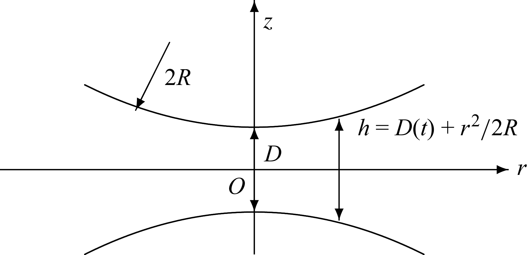
 2R
 D(t)

 ZEK(D~
 D~,α
 δ=0
 K∈(0.01,0.1,1,10)
 ZEK
 D~
 α=100
 δ=0
 K
 K=0.01
 K=0.01
 α=0.01
 K
 α2/2KD~

 D~H=D~/(1+ZEK/ZRey)
 D~
 K=0.01
 δ=0
 α
 D~H=D~−2b~
 b
 b~=ζ~2/8bee
 K
 α

 f~EK=ZEKD~/6
 D~=D/2ℓD
 α=100
 δ=0
 K
 f~EK
 K=0.01
 f~EK
 D~
 K=0.1
 δ=0
 α
 f~EK
 α≥10
 K(1−δ)
 δ∈(−0.7,−0.3,0,0.3,0.7)
 K
 K
 δ
 [K(1−δ)]−1

 ZDK
 β=Kω/4ωc
 D~=1
 α=10
 K=1
 ω0/ωc=4β0/K
 Re(ZDK)=Im(ZDK)
 D~=1
 K
 α
 ZDK
 D~
 K=1
 α=10
 ω/ωc
 β−1ZDK
 D~
 K=1
 α=10
 ω/ωc

 Re(ZDKhf)
 D~
 α=100
 K
 Re(ZDKhf)
 α
 K=0.1
 ZDLVO=ZDLVO/8πRn0kBT
 α=1
 α
 α=100

 f~DKℓf
 D~
 α=100
 K
 f~EK
 f~DKℓf
 K=0.1
 α
 f~EK
 K⋅f~DKℓf
 α
 K