



1 Introduction
Mass transfer between fluidic phases is central to many processes in nature and engineering such as liquid–liquid extraction (Rydberg Reference Rydberg2004),
 $\text{CO}_{2}$
sequestration (Loodts et al.
Reference Loodts, Thomas, Rongy and De Wit2014) or drying of films (Yiantsios et al.
Reference Yiantsios, Serpetsi, Doumenc and Guerrier2015). Frequently, the transport of a solute between immiscible liquids is accompanied by convection driven by two primary mechanisms: buoyancy (Rayleigh convection) and interfacial tension gradients (Marangoni convection). Investigations of Marangoni flows frequently employ the classical configuration of two stratified liquid layers stable to Rayleigh convection (Sternling & Scriven Reference Sternling and Scriven1959; Orell & Westwater Reference Orell and Westwater1962; Linde & Schwarz Reference Linde and Schwarz1963). Here, the transfer of surface-active solutes across the interface gives rise to complex, hierarchically structured patterns that are transient in time. The basic patterns of the non-oscillatory Marangoni instability, also including the highly nonlinear regimes, can be categorized into three classes (Linde, Schwarzenberger & Eckert Reference Linde, Schwarzenberger, Eckert, Rubio, Ryazantsev, Starov, Huang, Chetverikov, Arena, Nepomnyashchy, Ferrus and Morozov2013; Schwarzenberger et al.
Reference Schwarzenberger, Köllner, Linde, Boeck, Odenbach and Eckert2014): (i) polygonal Marangoni cells (named roll cells by Linde et al. (Reference Linde, Schwarzenberger, Eckert, Rubio, Ryazantsev, Starov, Huang, Chetverikov, Arena, Nepomnyashchy, Ferrus and Morozov2013)), (ii) relaxation oscillations or (iii) relaxation oscillation waves. Recently, the first two patterns were successfully reproduced in direct numerical simulations (Köllner et al.
Reference Köllner, Schwarzenberger, Eckert and Boeck2013, Reference Köllner, Schwarzenberger, Eckert and Boeck2015).
However, upon reversal of the direction of solute transport, these hierarchical Marangoni patterns are replaced by a new class of structures called ‘eruptions’, which obviously do not fit into the previous classification scheme. Eruptions refer to vigorous movements at the interface coupled to Rayleigh convection, as observed, for example, during the transport of acetic acid from ethyl acetate into water (Kroepelin & Neumann Reference Kroepelin and Neumann1957). Eruptions are not a rare event: similar experimental observations were reported by Orell & Westwater (Reference Orell and Westwater1962), Bakker, van Buytenen & Beek (Reference Bakker, van Buytenen and Beek1966) and Berg & Morig (Reference Berg and Morig1969). Further, Schwarz (Reference Schwarz1968) described their occurrence for more than 20 liquid/liquid systems with mass transfer of an organic solute. At an extended interface, eruptions are inherently coupled to erratic circular spreading motions (called ‘Spreitungen’ in German) as worked out by Schwarz (Reference Schwarz1968, Reference Schwarz1970) in the material system water + 1-propanol/cyclohexanol. Due to its disorganized appearance, this convective regime has so far resisted a deeper analysis, and its patterns have often been placed in the category ‘interfacial turbulence’.
The first formal, theoretical attempt to describe such a system was carried out in the linear stability analysis of Imaishi, Fujinawa & Tadaki (Reference Imaishi, Fujinawa and Tadaki1980). Considering the growth of oscillatory perturbations, they concluded that the eruptions might result from an interplay of the counteracting Rayleigh and Marangoni effects.
Mass transfer studies in droplet geometries also showed that the coupling of Rayleigh convection with a counteracting Marangoni effect can lead to certain oscillatory flow patterns. However, the distinct geometry of a droplet, i.e. the diameter as a distinguishing length scale and the type of the surrounding phase, are crucial for the specific hydrodynamic pattern emerging. For example, Lappa & Piccolo (Reference Lappa and Piccolo2004) observed structures resembling the eruptions in the vicinity of dissolving droplets with an imposed vertical temperature gradient, which they called ‘shooting’. Droplets dissolving in binary systems are susceptible to an irregular Marangoni convection, triggered by the introduction of surfactants. Without surfactants, only buoyant convection is present (Agble & Mendes-Tatsis Reference Agble and Mendes-Tatsis2000). In the studies of Kostarev et al. (Reference Kostarev, Shmyrov, Zuev and Viviani2011) and Schwarzenberger et al. (Reference Schwarzenberger, Aland, Domnick, Odenbach and Eckert2015a ), such a coupling leads to regular oscillations for droplets subjected to a concentration gradient.
A transfer of these insights to classical layered mass transfer systems is hardly possible since a restricting length scale, such as the droplet diameter, is absent here. For miscible two-layer systems, the full diversity of patterns resulting from buoyancy-driven instabilities recently received a systematic characterization (Trevelyan, Almarcha & De Wit Reference Trevelyan, Almarcha and De Wit2011). However, due to the additional effects of interfacial tension for the immiscible case considered here, a deeper understanding of the underlying cause of eruptions has been lacking up to now. With the aim of resolving this deficiency, an example of a mass transfer system is analysed in the present paper via simulation and experiment. In contrast to our prior studies (Köllner et al. Reference Köllner, Schwarzenberger, Eckert and Boeck2013, Reference Köllner, Schwarzenberger, Eckert and Boeck2015), the system is chosen such that it is stable with respect to stationary Marangoni instability but susceptible to Rayleigh convection on both sides of the interface. Based on this configuration, we show that the eruptions result from a two-step process. Rayleigh convection continuously produces localized regions of elevated concentration at the interface, which in turn trigger a vigorous Marangoni flow.
2 Methods
2.1 Experimental set-up
Similar to Schwarz (Reference Schwarz1970), water + 2-propanol/cyclohexanol is used as the material system. It is prepared as follows. A separating funnel is filled with water and cyclohexanol and the mixture is agitated for sufficiently long until the binary phases are in equilibrium. After separating the two phases, 2-propanol is dissolved in the water-rich phase with a volume concentration of 2.5 vol.%. The two phases are then injected into separate glass cuvettes with an inner size of
 $L\times W\times H=60~\text{mm}\times 60~\text{mm}\times 20~\text{mm}$
. To start mass transfer across the interface, the phases are joined by sliding the top cuvette including the lighter organic phase over the aqueous phase. This procedure of superposition (referred to as layering) was described in detail in Köllner et al. (Reference Köllner, Schwarzenberger, Eckert and Boeck2013). The start of the mass transfer experiment (
 $t_{exp}=0$
) is regarded as the time when the two phases come into contact for the first time. The subsequent cautious sliding of the layers against each other took 20 s.
A shadowgraph optics using parallel light aligned with the vertical direction is used to visualize the structures in the concentration field. The experimental shadowgraph images
 $s_{exp}(x,y)$
result from the deflection of light that is caused by the dependence of the refractive index on solute concentration. Furthermore, the optical flow field
 $\boldsymbol{u}_{of}$
is calculated from the shadowgraph images to capture the dynamics of the highly unsteady pattern. For that purpose, a commercial particle image velocimetry (PIV) tool ‘PivView2C’ (Willert Reference Willert2013) is applied, which detects the moving solute fronts as ‘tracers’.
2.2 Two-layer model
Our model considers two superposed immiscible, isothermal liquid phases. The kinematic viscosity, diffusivity of 2-propanol and height of the layer
 $i$
are
 ${\it\nu}^{(i)}$
,
 $D^{(i)}$
and
 $d^{(i)}$
. It is assumed that the interfacial tension
 ${\it\sigma}$
and density
 ${\it\rho}^{(i)}$
in layer
 $i$
decrease linearly with the concentration of 2-propanol as
 ${\it\rho}^{(i)}={\it\rho}_{ref}^{(i)}+{\it\rho}_{ref}^{(i)}{\it\beta}_{c}^{(i)}c^{(i)}c_{0}$
and
 ${\it\sigma}={\it\sigma}_{ref}+{\it\sigma}_{ref}{\it\alpha}_{c}c^{(1)}c_{0}$
relative to their values without 2-propanol,
 ${\it\rho}_{ref}^{(i)}$
and
 ${\it\sigma}_{ref}$
. In these material laws, the initial concentration of 2-propanol in the aqueous phase, the expansion coefficients, the coefficient of change in interfacial tension and the non-dimensional concentration are denoted by
 $c_{0}$
,
 ${\it\beta}_{c}^{(i)}$
,
 ${\it\alpha}_{c}$
and
 $c^{(i)}$
. The estimation of material parameters is given in the supplementary material available at http://dx.doi.org/10.1017/jfm.2016.63, which also includes the mathematical model. As reference units of length, time, velocity, pressure and concentration we use
 $d^{(1)}=20$
mm,
 $(d^{(1)})^{2}/{\it\nu}^{(1)}=333.3$
s,
 ${\it\nu}^{(1)}/d^{(1)}=60~{\rm\mu}\text{m}~\text{s}^{-1}$
,
 ${\it\rho}_{ref}^{(1)}({\it\nu}^{(1)})^{2}/(d^{(1)})^{(2)}=3.59~{\rm\mu}\text{Pa}$
and
 $c_{0}=0.32~\text{mol}~\text{l}^{-1}$
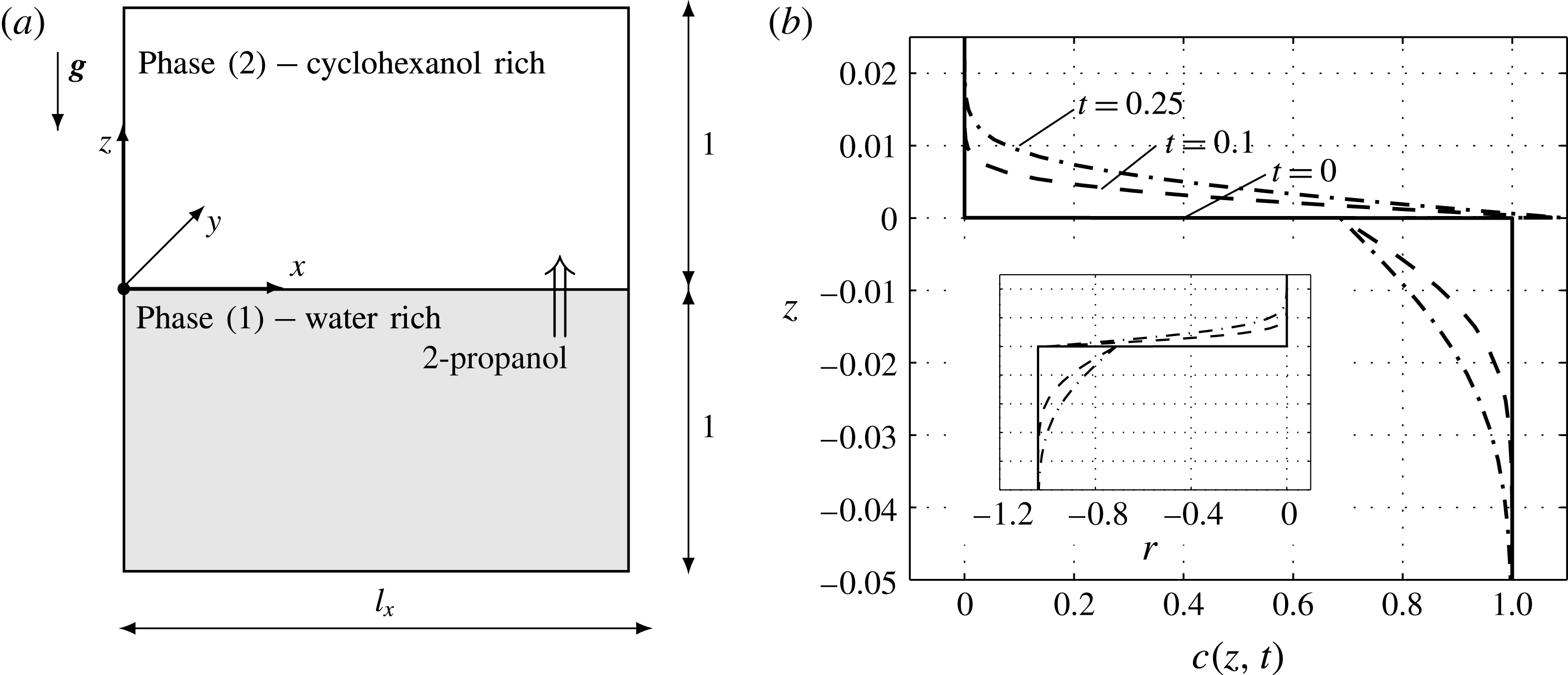
. Figure 1(a) sketches the cubic computational domain with horizontal dimensions of
 $l_{x}=l_{y}=0.75$
and vertical dimensions of
 $-1\leqslant z\leqslant 0$
for the lower water-rich phase and
 $0\leqslant z\leqslant 1$
for the upper cyclohexanol-rich phase.
Employed two-layer system: (a) sketch of the numerical domain, (b) simulated concentration profiles for pure diffusion, i.e.
 $G=Ma=0$
with an inset showing the variation of density
 $r=(c^{(i)}{\it\beta}_{c}^{(i)}{\it\rho}_{ref}^{(i)}/{\it\rho}_{ref}^{(1)})\times 100$
for the same times and vertical range (including identical grid line positions).
The momentum transport is modelled by the incompressible Navier–Stokes–Boussinesq equations and the solute transport by an advection–diffusion equation. At the plane interface, the partition of solute is governed by a Henry condition, and interfacial tension effects are introduced by the Marangoni shear stress balance. The present model equations are identical to the ones used in our previous investigation (Köllner et al.
Reference Köllner, Schwarzenberger, Eckert and Boeck2013). Non-dimensional velocity is denoted by
 $\boldsymbol{u}^{(i)}$
. According to the experimental set-up, no-slip and impermeable boundary conditions are imposed for the solid walls at the bottom and top. The
 $x$
–
 $y$
directions are periodic.
The arising non-dimensional groups and their actual values for a concentration of
 $c_{0}=0.32~\text{mol}~\text{l}^{-1}$
are the Marangoni number
 $Ma=c_{0}{\it\alpha}_{c}{\it\sigma}_{ref}d^{(1)}/({\it\rho}^{(1)}{\it\nu}^{(1)}D^{(1)})=-0.68\times 10^{7}$
, the Schmidt number in the aqueous phase
 $Sc^{(1)}={\it\nu}^{(1)}/D^{(1)}=1348$
, the Grashof number
 $G=c_{0}{\it\beta}_{c}^{(1)}g(d^{(1)})^{3}/({\it\nu}^{(1)})^{2}=-1.81\times 10^{5}$
, the partition coefficient
 $H=c_{eq}^{(2)}/c_{eq}^{(1)}=1.6$
, the ratio of densities
 ${\it\rho}={\it\rho}_{ref}^{(2)}/{\it\rho}_{ref}^{(1)}=0.96$
, the ratio of kinematic viscosities
 ${\it\nu}={\it\nu}^{(2)}/{\it\nu}^{(1)}=20.74$
, the ratio of diffusivities
 $D=D^{(2)}/D^{(1)}=0.082$
and the ratio of expansion coefficients
 ${\it\beta}_{c}^{(2)}/{\it\beta}_{c}^{(1)}=0.92$
.
2-propanol is initially dissolved only in the bottom layer, i.e.
 $c^{(1)}(t=0,x,y,z)=1$
,
 $c^{(2)}(t=0,x,y,z)=0$
. To trigger convection, the velocity field is initialized (
 $t=0$
) with a random noise of small magnitude: we set the grid values of vertical velocity
 $u_{z}^{(i)}(x_{l},y_{m},z_{k})$
and the vertical vorticity
 $\boldsymbol{{\rm\nabla}}\times \boldsymbol{u}^{(i)}(x_{l},y_{m},z_{k})\boldsymbol{\cdot }\boldsymbol{e}_{z}$
as uniformly distributed in the interval from 0 to
 $10^{-3}$
, and zero mean flow. The representation of the velocity field by the vertical velocity, the vertical vorticity and the horizontally averaged velocity component (mean flow) is detailed by Boeck et al. (Reference Boeck, Nepomnyashchy, Simanovskii, Golovin, Braverman and Thess2002).
The shadowgraph technique used in the experiments is mimicked by averaging the horizontal Laplacian of the concentration distribution over both layers (Merzkirch Reference Merzkirch1987),
 $s(x,y)=0.5\int _{[-1,1]}(\partial _{x}^{2}+\partial _{y}^{2})c(\boldsymbol{x},t)\,\text{d}z$
. A more accurate model of the shadowgraph technique could be used by taking into account the derivative of the refractive index with respect to the 2-propanol concentration for each layer separately, i.e.
 ${\it\kappa}^{(i)}=\partial n^{(i)}/\partial c^{(i)}$
. However, we keep the simpler formulation since those material properties
 ${\it\kappa}^{(i)}$
have not been measured, and for the observation of eruptive flow structures the top layer contributes clearly more due to lower diffusivity there.
The numerical method rests on a pseudospectral algorithm using a Fourier expansion in the
 $x{-}y$
direction with
 $N_{x}=1024,N_{y}=1024$
modes and a Chebyshev expansion in the
 $z$
dimension with polynomial degree of
 $N_{z}^{(1)}=256$
and
 $N_{z}^{(2)}=512$
. The present code has been used and validated in previous studies (Boeck et al.
Reference Boeck, Nepomnyashchy, Simanovskii, Golovin, Braverman and Thess2002; Köllner et al.
Reference Köllner, Schwarzenberger, Eckert and Boeck2013), where details can be found. The time step is adapted such that the grid Courant–Friedrichs–Lewy number is in the range of 0.1–0.2. Additionally, the time step is restricted to values smaller than
 $10^{-3}$
.
3 Numerical and experimental results
Before we turn to the full model, let us consider the case when Rayleigh and Marangoni effects are disregarded, i.e.
 $Ma=G=0$
. Then solute is transported by diffusion only, which is shown by solute profiles for successive times in figure 1(b). This base state is known to be stable with respect to the stationary Marangoni instability (Sternling & Scriven Reference Sternling and Scriven1959) because 2-propanol lowers the interfacial tension and diffuses faster in the phase that delivers solute. However, since 2-propanol decreases the density in both phases, a less dense concentration boundary layer develops above the interface and a denser one below the interface, cf. inset with variation of density
 $r(z)$
in figure 1(b). This density configuration is susceptible to a Rayleigh instability that leads to buoyant convection.
Temporal evolution of convection in the simulation: (a) r.m.s. velocities, (b) horizontally averaged velocity at three instants of time.
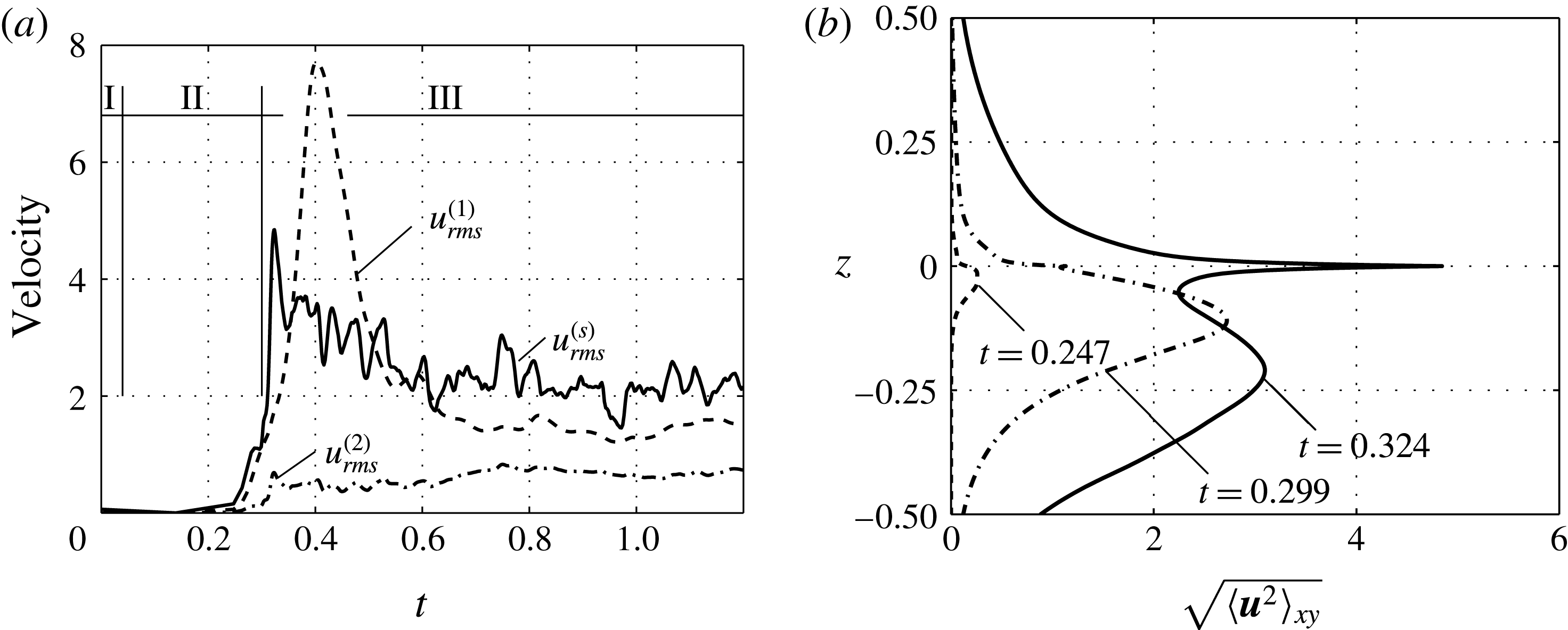
For the full model, figure 2(a) shows the root-mean-square velocity
 $u_{rms}^{(i)}$
in each layer and at the interface
 $u_{rms}^{(s)}=\sqrt{\langle \boldsymbol{u}^{2}(x,y,z=0,t)\rangle _{xy}}$
. A clear division into three regimes can be recognized. Regime I (
 $0<t\lesssim 0.04$
) refers to the diffusive base state, which is free of convection. The diffusive regime ends with the onset of the primary Rayleigh instability. We defined the time of onset as the earliest time for which the average of r.m.s. velocities
 $(u_{rms}^{(1)}+u_{rms}^{(2)})/2$
is growing. Additional simulations with initial amplitudes that were varied over several orders of magnitude all show onset times in the range of
 $0.04<t<0.05$
.
The growth of the Rayleigh instability governs regime II (
 $0.04\leqslant t<0.3$
). It lasts until the growth of
 $u_{rms}^{(s)}(t)$
stops for a moment. At this point, the eruptive regime III (
 $0.3\leqslant t$
) is initiated. The interfacial velocity grows rapidly to reach a maximum at
 $t=0.32$
. The intense interfacial flow can also be noted as a high peak at
 $z=0$
in the corresponding velocity profile (
 $t=0.324$
) in figure 2(b). After this vivid initial phase, regime III reaches a chaotic state that changes on a slower time scale, i.e. the changes in
 $u_{rms}^{(i)}$
and
 $u_{rms}^{(s)}$
are less pronounced in figure 2(a). Regimes II and III are the focus of this work.
3.1 Regime II: primary Rayleigh instability
As a result of the density variation, both layers are prone to Rayleigh convection. However, in the lower layer (1), convection is more pronounced (see the velocity data in figure 2) due to smaller viscosity and a thicker boundary layer there. Figure 3(a) shows the convection structures near the interface by plotting the concentration and velocity field in a vertical plane
 $y=0.25$
at
 $t=0.299$
. Solutal plumes composed of denser fluid due to depletion in 2-propanol sink downward in the lower layer, whereas less dense fluid rises quite slowly in the top layer.
Onset of convection in the simulation: (a) concentration and velocity field at a plane
 $y=0.25$
for
 $t=0.299$
, (b) space–time plot of interfacial concentration
 $c^{(1)}(x,y=0.25,z=0,t)$
. The dashed line in (b) indicates the time instant of the vertical cut in (a); the solid lines indicate time and space in figure 5(d–f).

At this stage, interfacial concentration is lowest at those places where mixed fluid departs from the interface, cf. figure 3(b). Hence, interfacial tension gradients, although small, are supporting the Rayleigh effect up to this time. The 3D pattern of the primary Rayleigh instability forms a polygonal pattern in a top view as shown in figure 4(a–c) (
 $t=0.299$
). The experimental pattern in figure 4(c,f,i) (see also supplementary movie 1) appears similar but does not possess this pronounced polygonal structure seen in the simulations. By comparison with the simulation data (see also supplementary movie 2), we observe that bright schlieren in the experiment result from solute transferred to the upper layer that remains localized near the interface (marked A). This less dense fluid rises only slowly all along the sides of the polygons in the upper layer. Before fluid rises preferably in the vertices, eruptions are initialized and break up this ordered polygonal pattern. Due to the faster Rayleigh convection in the lower layer, the downwelling plumes of denser fluid are mostly located at the
 $x,y$
position of a cell vertex, as observed in the synthetic shadowgram of the simulations (marked B). In the experimental shadowgram, these falling plumes are not clearly visible, probably because of a lower change in refractive index
 ${\it\kappa}^{(1)}$
(cf. § 2.2).
3.2 Eruptive regime III
As time progresses, the tips of density plumes depart from the interface and gradually encompass the bulk volume – see the further increase in
 $u_{rms}^{(1)}$
in figure 2. Simultaneously, the interfacial velocity
 $u_{rms}^{(s)}(t)$
shortly stops increasing around
 $t=0.30$
, indicating a qualitative change in the flow structure, i.e. the onset of eruptions.
Simulated and experimental patterns: (a,d,g) simulated isosurfaces
 $c^{(1)}=0.97$
,
 $c^{(2)}=0.2$
; (b,e,h) simulated synthetic shadowgraph image
 $s(x,y)$
in a domain of 0.75 (15 mm)
 $\times$
0.75 (15 mm); (c,f,i) experimental shadowgraph image of identical size. Circles with labels refer to the explanations in the text. The time of individual figures is as follows: (a,b)
 $t=0.299$
(99.8 s), (c)
 $t_{exp}=0.080$
(26.8 s), (d,e)
 $t=0.324$
(107.9 s), (f)
 $t_{exp}=0.105$
(34.9 s), (g,h)
 $t=0.904$
(301.33 s), (i)
 $t_{exp}=0.685$
(228.3 s).

It is most instructive to consider the interfacial concentration in figure 3(b): in regime II, the gradients
 $\partial _{x}c$
and therewith
 $\partial _{x}{\it\sigma}$
simply increase. After
 $t=0.30$
, however, they reverse their sign, causing the interfacial velocity
 $\boldsymbol{u}^{(s)}$
to reverse its direction locally due to the balance of Marangoni and viscous stresses. Finally, eruptions are manifested as expanding circular schlieren in the shadowgraph images of figure 4(d–f) (marked C).
Development of an eruption: (a–c) surface of
 $c^{(2)}=0.2$
including the cutting plane (triangles) of (d–f) numerical concentration and velocity field at
 $y=0.25$
, (g–i) numerical shadowgraph images
 $s(x,y)$
with interfacial velocity
 $\boldsymbol{u}(x,y,z=0,t)$
and (j–l) experimental shadowgraph images
 $s_{exp}(x,y)$
(same size as numerical) with optical flow
 $\boldsymbol{u}_{of}$
. The simulated images start at
 $t=0.3173$
, denoted by
 ${\it\tau}=0$
, and the experimental images start at
 $t_{exp}=0.3468$
(115.6 s), thus
 ${\it\tau}$
refers to the relative time that is matched: (a,d,g,j)
 ${\it\tau}=0$
, initialization; (b,e,h,k)
 ${\it\tau}=0.006$
, maximum speed; (c,f,i,l)
 ${\it\tau}=0.016$
, decay.

The evolution of a single eruption from both experiment and simulation is depicted as an example in figure 5; its position and time correspond to the three solid horizontal lines in figure 3(b). Figure 5 shows a sequence of isosurfaces
 $c^{(2)}=0.2$
(a–c), vertical cuts through the concentration and velocity fields at
 $y=0.25$
(d–f) and the corresponding synthetic shadowgram with interfacial velocity (g–i). For the experimental shadowgram with optical flow (j–l), an eruption of similar appearance is chosen. An eruption cycle proceeds in three characteristic stages. First (
 ${\it\tau}=0$
, left-hand column), eruptions are initialized at a specific point. The location of this point results from the complex interaction between the growing portions of solute-rich fluid in the upper layer and the downwelling plumes in the lower layer. In this process, the solute-rich fluid (in the upper phase) that gathered near the interface is transported towards the interface. It is manifested as a diverging radial motion in both experimental and numerical shadowgraph images. Second, the spreading motion accelerates by the continuing inflow of solute-rich fluid and adopts a state of maximum speed (
 ${\it\tau}=0.006$
, middle column). Third, the eruptions decay, i.e. the spreading of solute ceases by interfering with the neighbouring structures (
 ${\it\tau}=0.016$
, right-hand column).
After the eruptions have become established, the system dynamics appears rather chaotic but can be characterized by three features: (1) frequent emission of solutal plumes in the bottom layer, (2) the continuous presence of erratic interfacial motion (eruptions) and (3) the formation of larger portions of enriched fluid that slowly rise in the form of plumes in the top layer (marked D in figure 4). Two different stages of plume development can be distinguished. In the early stage, the plumes rise freely in the bulk (marked D1 in figure 4). Hence, they are observed as small circular schlieren that marginally change their position and size. In the late stage, the plumes hit the top wall and, therefore, appear as a distinctly growing circular pattern (marked D2 in figure 4).
Temporal evolution of convection: (a) averaged interfacial velocity and optical flow for simulations and experiments with offset time
 ${\rm\Delta}t=0.219$
, (b) volume-averaged concentration in layer 2 normalized by the equilibrium concentration.

For a quantitative comparison, we look at the temporal evolution of characteristic velocities from experiment and simulations. Therefore, the r.m.s. value of the optical flow
 $\bar{u}_{of}(t)=\sqrt{\langle \boldsymbol{u}_{of}^{2}(x,y,t)\rangle _{xy}}$
is calculated over the 15 mm
 $\times$
15 mm middle section of the experimental cuvette (also shown in figure 4). Simulations are represented by equally applying this method to the synthetic shadowgraph images
 $s(x,y)$
and by the actual interfacial velocity
 $u_{rms}^{(s)}(t)$
. These three quantities are plotted in figure 6(a). To match the onset of convection between experiment and simulation, an offset time of
 ${\rm\Delta}t=0.219$
was added to the experimental time
 $t_{exp}$
. All three velocity curves show the same characteristic behaviour: vigorous onset with subsequent decay in motion. The experimental flow appears accelerated. It is approximately twice as fast as the simulated optical flow. Furthermore, optical flow and interfacial velocity (of the simulation) seem to be well correlated, but interfacial velocity was roughly twice as high as the simulated optical flow.
Since eruptions are supposed to occur in several solvent systems relevant for chemical engineering, we finally address the impact of this regime on the mass transfer. The latter is quantified by the averaged solute concentration
 $\langle c^{(2)}\rangle _{xyz}$
normalized with the equilibrium concentration in the top layer
 $c_{eq}^{(2)}=H/(1+H)$
. Figure 6(b) shows this value for the full simulation (solid line), for a simulation without Marangoni effect (i.e. taking
 $Ma=0$
but keeping other parameters, dashed line) and for pure diffusion (dashed-dotted line). In general, convection enhances mass transport, as expected. Remarkably, the eruption regime shows the highest transferred amount of solute.
4 Discussion and outlook
The results presented in § 3 show that our simulations reproduce the key features of the patterns observed in our experiment remarkably well. The considered mass transfer system water + 2-propanol/cyclohexanol thereby serves as a representative example of various experimental systems displaying a specific phenomenon of interfacial convection, known as eruptions. On this basis, the so far poorly understood eruptive regime of mass transfer-driven Rayleigh–Marangoni convection can be deciphered as follows: eruptions are spontaneous circular spreading motions of surface-active solute along the interface in a system that is a priori stable with respect to a primary Marangoni instability. The unstable concentration distribution is provided by the preceding and sustained Rayleigh convection.
In the present system, Rayleigh convection is weaker in the accepting phase. Thus, enriched fluid portions are barely transported away from the interface, which causes an asymmetric distribution of solute that especially triggers eruptions. By their strong tangential motion, eruptions prevent the Rayleigh convection from appearing in persistent convection cells. In turn, the locus of buoyant plume emission is altered, which causes a stochastic occurrence of new eruptions in space and time.
In this view, the interplay of eruptions and buoyant convection can be regarded as an oscillatory flow state due to the ‘sign’ change in the velocity and the surface tension gradient at a fixed location. This change from Rayleigh to the Marangoni effect as the origin of the eruptions was already anticipated by Imaishi et al. (Reference Imaishi, Fujinawa and Tadaki1980) from the stability results of their linear model.
In contrast to Rayleigh convection, the effect of Marangoni convection is rather localized to a narrow zone near the interface. However, simulations without the Marangoni effect show a distinctly retarded transfer of solute compared to the presented case. This implies that the presence of interfacial tension gradients may play a crucial role in the prediction of mass transfer in systems with solutal Rayleigh convection, even for very large layers.
An exact reproduction of the early experimental phase was not fully achieved since the onset of convection and the layering procedure act on similar time scales, and the complex process of layering is not described by the simulation. By analysing the shadowgraph images in terms of optical flow, the simulations show a similar qualitative progression, but lower ‘interfacial’ velocities, approximately half the experimental value. A clear physical reason could not be identified due to the complexity of the physical system, the uncertainty of material properties and the numerous simplifications in the model equations, which are, however, necessary for an efficient numerical treatment. A similar relationship between experimental and simulated velocities was found for convection in Marangoni roll cells (Schwarzenberger et al. Reference Schwarzenberger, Köllner, Boeck, Odenbach, Eckert, Rahni, Karbaschi and Miller2015b ).
The question of for which physical parameters eruptions are to be expected deserves further studies. Circumstances for their occurrence are as follows. (1) A solute that lowers the interfacial tension (
 ${\it\alpha}_{c}<0$
) is to be transported from the layer with higher diffusivity to the layer with lower diffusivity, in our case
 $D<0$
. Otherwise, Marangoni convection is amplified (Sternling & Scriven Reference Sternling and Scriven1959). (2) Solute has to lower (increase) the density when transported upwards (downwards), i.e.
 ${\it\beta}_{c}^{(i)}<0$
in our case. What happens if the density is increasing in one phase but decreasing in the other phase upon addition of solute remains to be studied. (3) The characteristic Rayleigh number
 $Ra^{(i)}={\rm\Delta}c^{(i)}{\it\beta}_{c}^{(i)}gd^{(i)}/({\it\nu}^{(i)}D^{(i)})$
in layer (
 $i$
), here to be calculated with the actual difference in concentration between the interface and the undisturbed bulk
 ${\rm\Delta}c^{(i)}$
, has to be large enough. This is because the linear threshold for the onset of Rayleigh convection has to be exceeded; it is of the order of
 $10^{3}$
. Since the present study employs a system with large layer heights, i.e.
 $Ra^{(1)}\approx -8\times 10^{7}$
,
 $Ra^{(2)}\approx -2\times 10^{8}$
, we expect the influence of layer heights to be negligible for the eruptions. However, the effects of a finite layer size (especially for shallow layers) may prevent or alter the occurrence of eruptions (Imaishi et al.
Reference Imaishi, Fujinawa and Tadaki1980). (4) The Marangoni effect has to be strong enough compared to the buoyant convection. (5) Last, we are not aware that eruptions are observed in the case of thermal convection between two layers. Hence, we assume that the Schmidt number has to be distinctly larger than one. In this view, a comprehensive coverage of the rather large parameter space where eruptions may occur is an issue for further investigation.
Acknowledgements
Financial support by the Deutsche Forschungsgemeinschaft in the framework of Priority Program 1506 is gratefully acknowledged. Computing centre of TU Ilmenau is acknowledged for computing resources.
Supplementary material and movies
Supplementary material and movies are available at http://dx.doi.org/10.1017/jfm.2016.63.



