2. Preliminaries

In this section, we introduce some known results on the theory of geometric singular perturbation (see. e.g., [Reference Jones21]). Consider the system

(2.1)\begin{equation} \begin{cases} x_1'=f(x_1,x_2,\epsilon),\\ x_2'=\epsilon g(x_1,x_2,\epsilon), \end{cases} \end{equation}

where $'=\frac {{\rm d}}{{\rm d}t}$, $x_1\in \mathbb {R}^n$, $x_2\in \mathbb {R}^l$ and $\epsilon$ is a positive real parameter, $U\subseteq \mathbb {R}^{n+l}$ is open subset, and $I$ is an open subset of $\mathbb {R}$, containing $0$. $f$ and $g$ are $C^\infty$ on a set $U\times I$. Moreover, the $x_1$ (resp., $x_2$) variables are called fast (resp., slow) variables. Letting $\tau =\epsilon t$ which gives the following equivalent system

(2.2)\begin{equation} \begin{cases} \epsilon \dot{x_1}=f(x_1,x_2,\epsilon),\\ \dot{x_2}= g(x_1,x_2,\epsilon), \end{cases} \end{equation}

where $\cdot =\frac {{\rm d}}{{\rm d}\tau }$. We refer to $t$ (resp., $\tau$) as the fast time scale or fast time (resp., slow time scale or slow time). Each of the scalings is naturally associated with a limit as $\epsilon$ tend to zero. These limits are respectively given by

(2.3)\begin{equation} \begin{cases} x_1'=f(x_1,x_2,0),\\ x_2'=0, \end{cases} \end{equation}

and

(2.4)\begin{equation} \begin{cases} 0=f(x_1,x_2,0),\\ x_2'=g(x_1,x_2,0). \end{cases} \end{equation}

System (2.3) is called the layer problem and system (2.4) is reduced system.

3. Reduction of the model by geometric singular perturbation theory and dynamical system method

In this section, to consider the exact solutions of the unperturbed $(1+1)$-dimensional DLWE (1.3), we firstly reduce the model by GSP theory and dynamical system method. From the view of physical meanings, we only consider the case of $c>0$ in this paper.

By introducing the following transformations:

(3.1)\begin{equation} u(x,t)=\phi(\xi),\quad v(x,t)=\psi(\xi),\quad \xi=x-ct, \end{equation}

we obtain

(3.2)\begin{equation} \begin{aligned} & \frac{\partial u(x,t)}{\partial t}={-}c\phi_{\xi},\quad \frac{\partial v(x,t)}{\partial t}={-}c\psi_{\xi},\\ & \frac{\partial^{2 }u(x,t)}{\partial x^{2 }}=\phi_{\xi\xi},\quad \frac{\partial^{3 }u(x,t)}{\partial x^{3 }}=\phi_{\xi\xi\xi},\quad \frac{\partial^{4 }u(x,t)}{\partial x^{4 }}=\phi_{\xi\xi\xi\xi}, \end{aligned} \end{equation}

where $\phi _{\xi }$ and $\psi _{\xi }$ are the first order derivative with respect to $\xi$. And $\phi _{\xi \xi }$, $\phi _{\xi \xi \xi }$ and $\phi _{\xi \xi \xi \xi }$ means the second, third and fourth order derivative with respect to $\xi$, respectively.

Substituting (3.1) and (3.2) into (1.3), then system (1.3) is given by

(3.3)\begin{equation} \begin{cases} c \phi_{\xi}=\phi \phi_{\xi}+\psi_{\xi},\\ c \psi_{\xi}=\psi \phi_{\xi}+\phi \psi_{\xi}+\frac{1}{3}\phi_{\xi\xi\xi}-\varepsilon (\phi_{\xi\xi}+\phi_{\xi\xi\xi\xi}). \end{cases} \end{equation}

Integrating both sides of the first equation of system (3.3) once with respect to $\xi$ and letting the integration constant be zero yields

(3.4)\begin{equation} \psi(\xi)=c \phi(\xi)-\frac{1}{2}\phi^2(\xi). \end{equation}

We substitute (3.4) into the second equation of (3.3), then the coupled system (3.3) becomes the following ODE:

(3.5)\begin{equation} \frac{1}{3}\phi_{\xi\xi\xi}-\frac{3}{2}\phi^2\phi_{\xi}+3c \phi \phi_\xi-c^2\phi_\xi-\varepsilon (\phi_{\xi\xi}+ \phi_{\xi\xi\xi\xi})=0. \end{equation}

Integrating both sides on (3.5) once with respect to $\xi$ and rescaling $\epsilon =3\varepsilon$, it follows that

(3.6)\begin{equation} \phi_{\xi\xi}-\frac{3}{2}\phi^3+\frac{9}{2}c\phi^2-3c^2\phi-\epsilon(\phi_{\xi}+ \phi_{\xi\xi\xi})=g, \end{equation}

where $g$ is an integration constant ($g\in \mathbb {R}$).

Introducing new variables $\zeta =c\xi$, $z=\frac {\phi }{c}$ and $G=\frac {g}{c^3}$, equation (3.6) is equivalent to

(3.7)\begin{equation} -3z+\frac{9}{2}z^2-\frac{3}{2}z^3+\frac{{\rm d}^2z}{{\rm d}\zeta^2}-\epsilon\left(\frac{1}{c}\frac{{\rm d}z}{{\rm d}\zeta}+c\frac{{\rm d}^3z}{{\rm d}\zeta^3}\right)=G. \end{equation}

Obviously, equation (3.7) reduces to a three-dimensional system:

(3.8)\begin{equation} \begin{cases} \dfrac{{\rm d}z}{{\rm d}\zeta}=y,\\ \dfrac{{\rm d}y}{{\rm d}\zeta}=w,\\ \epsilon c\dfrac{{\rm d}w}{{\rm d}\zeta}={-}3z+\frac{9}{2}z^2-\dfrac{3}{2}z^3+w-\dfrac{\epsilon}{c}y-G, \end{cases} \end{equation}

where $\epsilon$ is a sufficiently small parameter such that $0<\epsilon \ll 1$. Therefore, the travelling wave solutions of equation (1.3) can be obtained by studying the corresponding orbits of system (3.8).

Obviously, system (3.8) is a singularly perturbed system described as ‘slow system.’ Rescaling $\zeta =\epsilon \eta$, we have the following equivalent ‘fast system’:

(3.9)\begin{equation} \begin{cases} \dfrac{{\rm d}z}{{\rm d}\eta}=\epsilon y,\\ \dfrac{{\rm d}y}{{\rm d}\eta}=\epsilon w,\\ c\dfrac{{\rm d}w}{{\rm d}\eta}={-}3z+\dfrac{9}{2}z^2-\dfrac{3}{2}z^3+w-\dfrac{\epsilon}{c}y-G. \end{cases} \end{equation}

Let $\epsilon =0$ in system (3.8) and (3.9). Then, the corresponding reduced system is given by

(3.10)\begin{equation} \begin{cases} \dfrac{{\rm d}z}{{\rm d}\zeta}=y,\\ \dfrac{{\rm d}y}{{\rm d}\zeta}=w,\\ 0={-}3z+\dfrac{9}{2}z^2-\dfrac{3}{2}z^3+w-G, \end{cases} \end{equation}

and the layer system is

(3.11)\begin{equation} \begin{cases} \dfrac{{\rm d}z}{{\rm d}\eta}=0,\\ \dfrac{{\rm d}y}{{\rm d}\eta}=0,\\ c\dfrac{{\rm d}w}{{\rm d}\eta}={-}3z+\frac{9}{2}z^2-\dfrac{3}{2}z^3+w-G, \end{cases} \end{equation}

which admits a two-dimensional critical manifold as follows

(3.12)\begin{equation} M_0=\left\{(z,y,w) \in \mathbb{R}^3|w=3z-\frac{9}{2}z^2+\frac{3}{2}z^3+G \right\}. \end{equation}

Suppose $A$ to be the linearized matrix of system (3.11), then it is given by

(3.13)\begin{equation} A=\left(\begin{array}{ccc} 0 & 0 & 0 \\ 0 & 0 & 0 \\ \dfrac{-3+9z-\dfrac{9}{2}z^2}{c} & 0 & \dfrac{1}{c} \\ \end{array}\right), \end{equation}

that the eigenvalues of A are $0$, $0$ and $\frac {1}{c}$. Thus, $M_0$ is a normally hyperbolic invariant manifold (see definitions 2.1 and 2.2). There exists a two-dimensional slow submanifold $M_\epsilon$ which is $C^1$ $O(\epsilon )$ close to $M_0$ (see lemma 2.3). The invariant submanifold $M_\epsilon$ is represented by

(3.14)\begin{align} M_\epsilon& =\left\{(z,y,w) \in \mathbb{R}^3|w=3z-\frac{9}{2}z^2+\frac{3}{2}z^3+G\right.\nonumber\\ & \left. \quad +\,\epsilon\left[cy\left(\frac{9}{2}z^2-9z+3+\frac{1}{c^2}\right)\right]+O(\epsilon^2) \right\}. \end{align}

The dynamical behaviour of slow system (3.8) or fast system (3.9) is governed by

(3.15)\begin{equation} \begin{cases} \dfrac{{\rm d}z}{{\rm d}\zeta}=y,\\ \dfrac{{\rm d}y}{{\rm d}\zeta}=3z-\dfrac{9}{2}z^2+\frac{3}{2}z^3+G+\epsilon[cy(\dfrac{9}{2}z^2-9z+3+\dfrac{1}{c^2})]+O(\epsilon^2). \end{cases} \end{equation}

Obviously, the unperturbed system (3.15)$\mid _{\epsilon =0}$ admits homoclinic, heteroclinic and periodic orbits with the parameter $G$ taking different values. By the bifurcation theory of planar dynamical systems (see [Reference Li22]), we have the following proposition of unperturbed system (3.15)$\mid _{\epsilon =0}$:

Proposition 3.1

1. (i) If $\mid G\mid >\frac {\sqrt 3}{3}$, there exists a single saddle point [see figures 1(a) or (g)].

2. (ii) If $\mid G\mid =\frac {\sqrt 3}{3}$, there exist a saddle point and a cusp point [see figures 1(b) or (f)].

3. (iii) If $G=0$, there exist two saddle points $(0,0)$ and $(2,0)$, and a centre point $(1,0)$. It has two heteroclinic orbits surrounding the centre point $(1,0)$ to two saddle points $(0,0)$ and $(2,0)$ [see figure 1(d)].

4. (iv) If $0<\mid G\mid <\frac {\sqrt 3}{3}$, there exist a saddle point and a centre point. It has a homoclinic orbit surrounding the centre point to one saddle point [see figures 1(c) or (e)].

Figure 1.

The bifurcation and phase portraits of unperturbed system (3.15)$\mid _{\epsilon =0}$.

Assume that $z(\zeta )$ is a solution of equation (3.7) satisfying $\lim \limits _{\zeta \longrightarrow \infty }z(\zeta )={\kappa }$, thus $u(x,t)=cz(\zeta )=cz[c(x-ct)]$ is a solitary wave solution or a kink wave solution of equation (3.7).

For $-\frac {\sqrt 3}{3}< G\leq 0$ and $0\leq G<\frac {\sqrt 3}{3}$, the unperturbed system (3.15)$\mid _{\epsilon =0}$ admits a saddle point defined by $S_0({\kappa },0)$. We know that $G=-\left (3{\kappa }-\frac {9}{2}{\kappa }^2+\frac {3}{2}{\kappa }^3\right )$, then we obtain $1+\frac {\sqrt 3}{3}<{\kappa }\leq 2$ for $G\in \left (-\frac {\sqrt 3}{3},0\right ]$ and $0\leq {\kappa }<1-\frac {\sqrt 3}{3}$ for $G\in \left [0,\frac {\sqrt 3}{3}\right )$, respectively. We can regard ${\kappa }$ as a bifurcation parameter to find the homoclinic orbits of system (3.15). Therefore, we rewrite system (3.15), that is:

(3.16)\begin{equation} \begin{cases} \dfrac{{\rm d}z}{{\rm d}\zeta}=y,\\ \dfrac{{\rm d}y}{{\rm d}\zeta}=3z-\dfrac{9}{2}z^2+\dfrac{3}{2}z^3-\left(3{\kappa}-\dfrac{9}{2}{\kappa}^2+\dfrac{3}{2}{\kappa}^3\right)\\ \quad +\,\epsilon\left[cy\left(\dfrac{9}{2}z^2-9z+3+\dfrac{1}{c^2}\right)\right]+O(\epsilon^2). \end{cases} \end{equation}

4. Travelling wave solutions of equation (1.3)$\mid _{\varepsilon =0}$

In this section, we study the solitary and kink (anti-kink) wave solutions of equation (1.3)$\mid _{\varepsilon =0}$. By dynamical method, we consider the travelling wave solution of system (3.16)$\mid _{\epsilon =0}$ with ${\kappa }\in \left [0,1-\frac {\sqrt 3}{3}\right )\cup \left (1+\frac {\sqrt 3}{3},2\right ]$. The unperturbed system (3.16) is of the form:

(4.1)\begin{equation} \begin{cases} \dfrac{{\rm d}z}{{\rm d}\zeta}=y,\\ \dfrac{{\rm d}y}{{\rm d}\zeta}=3z-\dfrac{9}{2}z^2+\dfrac{3}{2}z^3-\left(3{\kappa}-\dfrac{9}{2}{\kappa}^2+\dfrac{3}{2}{\kappa}^3\right). \end{cases} \end{equation}

It is easy to obtain the first integral of system (4.1), it is given by

(4.2)\begin{equation} H(z,y)=\frac{1}{2}y^2-\frac{3}{8}z^4+\frac{3}{2}z^3-\frac{3}{2}z^2+\left(\frac{3}{2}{\kappa}^3-\frac{9}{2}{\kappa}^2+3{\kappa}\right)z. \end{equation}

The homoclinic orbit $\Gamma ({\kappa })$ to the saddle $({\kappa },0)$ is defined by

(4.3)\begin{align} H(z,y)& =\frac{1}{2}y^2-\frac{3}{8}z^4+\frac{3}{2}z^3-\frac{3}{2}z^2+\left(\frac{3}{2}{\kappa}^3-\frac{9}{2}{\kappa}^2+3{\kappa}\right)z\nonumber\\ & =\frac{9}{8}{\kappa}^4-3{\kappa}^3+\frac{3}{2}{\kappa}^2. \end{align}

And the heteroclinic orbits $\Upsilon ({\kappa })_{\pm }$ (where $\pm$ represents upper and lower branch curves) to the two saddle points $(0,0)$ and $(2,0)$, namely, ${\kappa }=0$ or ${\kappa }=2$, the heteroclinic curve is determined by

(4.4)\begin{equation} \begin{array}{l} H(z,y)=\dfrac{1}{2}y^2-\dfrac{3}{8}z^4+\dfrac{3}{2}z^3-\dfrac{3}{2}z^2=0. \end{array} \end{equation}

4.1. Solitary wave solutions of equation (1.3)$\mid _{\varepsilon =0}$

By (4.3) and proposition 3.1(iv), we can obtain the expression of $y$ as follows:

(4.5)\begin{align} y& ={\pm} \sqrt{\frac{3}{4}z^4-3z^3+3z^2-(3{\kappa}^3-9{\kappa}^2+6{\kappa})z+\frac{9}{4}{\kappa}^4-6{\kappa}^3+3{\kappa}^2}\nonumber\\ & ={\pm} \sqrt{\frac{3}{4}(z-{\kappa})^2(z-z_+)(z-z_-)}, \end{align}

where $z_{\pm }=-{\kappa }+2\pm \sqrt {-2{\kappa }^2+4{\kappa }}$. It can be seen that $z_-< z_+<{\kappa }$ for $1+\frac {\sqrt 3}{3}<{\kappa }<2$ [see figure 1(c)] and ${\kappa }< z_-< z_+$ for $0<{\kappa }<1-\frac {\sqrt 3}{3}$ [see figure 1(e)].

Since $\frac {{\rm d}z}{{\rm d}\zeta }=y$, it implies

(4.6)\begin{equation} \frac{{\rm d}z}{{\rm d}\zeta}={\pm} \sqrt{\frac{3}{4}(z-{\kappa})^2(z-z_+)(z-z_-)}, \end{equation}

which yields

(4.7)\begin{equation} \zeta={\pm} \int_{z_+}^{z}\frac{1}{\sqrt{\frac{3}{4}(s-{\kappa})^2(s-z_+)(s-z_-)}}\,{\rm d}s,\quad \left(1+\frac{\sqrt3}{3}<{\kappa}<2\right), \end{equation}

and

(4.8)\begin{equation} \zeta={\pm} \int_{z_-}^{z}\frac{1}{\sqrt{\frac{3}{4}(s-{\kappa})^2(z_+{-}s)(z_-{-}s)}}\,{\rm d}s,\quad \left(0<{\kappa}<1-\frac{\sqrt3}{3}\right). \end{equation}

Thus, for $1+\frac {\sqrt 3}{3}<{\kappa }<2$, the parametric representation of the dark solitary wave of system (3.16)$|_{\epsilon =0}$ can be obtained by [see figure 2(a)]

(4.9)\begin{equation} z(\zeta)={-}\frac{2(6{\kappa}^2-12{\kappa}+4)}{2\text{cosh}\left(\frac{1}{2}\sqrt{18{\kappa}^2-36 {\kappa}+12}\zeta\right)\sqrt{-2{\kappa}^2+4{\kappa}}+4{\kappa}-4}. \end{equation}

Then, it corresponds to a dark solitary wave solution [see figure 2(b)] of equation (1.3)$\mid _{\varepsilon =0}$ is given by:

(4.10)\begin{equation} u(x,t)={-}\frac{2(6{\kappa}^2-12{\kappa}+4)c}{2\text{cosh}\left[\frac{1}{2}\sqrt{18{\kappa}^2-36 {\kappa}+12}c(x-ct)\right]\sqrt{-2{\kappa}^2+4{\kappa}}+4{\kappa}-4}. \end{equation}

For $0<{\kappa }<1-\frac {\sqrt 3}{3}$, the expression of the bright solitary wave of system (3.16)$|_{\epsilon =0}$ can be obtained by [see figure 3(a)]

(4.11)\begin{equation} z(\zeta)={-}\frac{2(6{\kappa}^2-12{\kappa}+4)}{4{\kappa}-4-2\text{cosh}\left(\frac{1}{2}\sqrt{18{\kappa}^2-36 {\kappa}+12}\zeta\right)\sqrt{-2{\kappa}^2+4{\kappa}}}. \end{equation}

The bright solitary wave solution of equation (1.3)$\mid _{\varepsilon =0}$ [see figure 3(b)] is of the form

(4.12)\begin{equation} u(x,t)={-}\frac{2(6{\kappa}^2-12{\kappa}+4)c}{4{\kappa}-4-2\text{cosh}\left[\frac{1}{2}\sqrt{18{\kappa}^2-36 {\kappa}+12}c(x-ct)\right]\sqrt{-2{\kappa}^2+4{\kappa}}}. \end{equation}

Figure 2.

Dark solitary wave of system (3.16)$|_{\epsilon =0}$ and exact solution of equation (1.3)$\mid _{\varepsilon =0}$ for $c=0.5$ and ${\kappa }=1.7$. (a) Dark solitary wave. (b) Exact solution.

Figure 3.

Bright solitary wave of system (3.16)$|_{\epsilon =0}$ and exact solution of equation (1.3)$\mid _{\varepsilon =0}$ for $c=0.5$ and ${\kappa }=0.3$. (a) Bright solitary wave (b) Exact solution.

In summary, we give the theorem as follows.

Theorem 4.1 For any wave speed $c>0$ and ${\kappa }\in \left (0,1-\frac {\sqrt 3}{3}\right )\cup \left (1+\frac {\sqrt 3}{3},2\right )$, equation (1.3) $\mid _{\varepsilon =0}$ has solitary wave solutions given by (4.10) or (4.12).

4.2. Kink and anti-kink wave solutions of equation (1.3)$\mid _{\varepsilon =0}$

According (4.4) and proposition 3.1(iii), we can obtain the expression of $y$ as follows:

(4.13)\begin{equation} y={\pm} \sqrt{\frac{3}{4}z^4-3z^3+3z^2}={\pm} \sqrt{\frac{3}{4}(z-0)^2(2-z)^2}={\pm} \frac{\sqrt3}{2}z(z-2). \end{equation}

Similarly, due to $\frac {{\rm d}z}{{\rm d}\zeta }=y$, we have

(4.14)\begin{equation} \zeta={\pm} \int_{1}^{z}\frac{1}{\frac{\sqrt3}{2}s(s-2)}\,{\rm d}s. \end{equation}

For $\kappa =0$ or $\kappa =2$, the expression of the kink or anti-kink wave of system (3.16)$|_{\epsilon =0}$ can be obtained by [see figures 4(a) and (c)]

(4.15)\begin{equation} z(\zeta)=\frac{2c}{1+{\rm e}^{{\pm}\sqrt3c\zeta}}. \end{equation}

Therefore, we obtain the following kink and anti-kink wave solutions (see figures 4(b) and (b)]:

(4.16)\begin{equation} u(x,t)=\frac{2c}{1+{\rm e}^{{\pm}\sqrt3c(x-ct)}}. \end{equation}

Figure 4.

Kink and anti-kink wave of system (3.16)$|_{\epsilon =0}$. Kink and anti-kink wave solutions of equation (1.3)$\mid _{\varepsilon =0}$ for $c=0.5$. (a) Kink wave (b) Kink wave solution (c) Anti-kink wave (d) Anti-kink wave solution.

Based on above analysis, we have the following theorems:

Theorem 4.2 For any wave speed $c>0$ and $\kappa =0$ or $\kappa =2$, equation (1.3) $\mid _{\varepsilon =0}$ has kink or anti-kink solutions given by (4.16).

5. Bifurcations of the travelling wave solutions for the perturbed equation (1.3)

In this section, before stating our main results on the existence of the solitary and kink wave solutions for the perturbed equation (1.3), denote

(5.1)\begin{align} c_1(\kappa)\Big|_{\kappa\in\left(0,1-\frac{\sqrt3}{3}\right)}& =\frac{\sqrt{15}}{3}\left[\left(6\text{ln}2{\kappa}^3+6{\kappa}^3\text{ln}\left(\sqrt{6{\kappa}^2-12{\kappa}+4}+2{\kappa}-2\right)-18\text{ln}2{\kappa}^2\right.\right.\nonumber\\ & \quad-18{\kappa}^2\text{ln}\left(\sqrt{6{\kappa}^2-12{\kappa}+4}+2{\kappa}-2\right)+12\text{ln}2{\kappa}\nonumber\\ & \quad\left.+12{\kappa}\text{ln}\left(\sqrt{6{\kappa}^2-12{\kappa}+4}+2{\kappa}-2\right)+2\sqrt{6{\kappa}^2-12{\kappa}+4}\right]\nonumber\\ & \quad-\sqrt3 {\kappa}\left[2{\kappa}^2\text{ln}\left(-\sqrt{2{\kappa}-{\kappa}^2}\right)\right.\nonumber\\ & \left.\quad +3\text{ln}2{\kappa}^2-6{\kappa}\text{ln}\left(-\sqrt{2{\kappa}-{\kappa}^2}\right)-9\text{ln}2{\kappa}\right.\nonumber\\ & \quad\left.+4\text{ln}\left(-\sqrt{2{\kappa}-{\kappa}^2}\right)+6\text{ln}2\right)\big/\left(27{\kappa}^4 \sqrt{6{\kappa}^2-12{\kappa}+4}\right.\nonumber\\ & \quad+30 {\kappa}^3\text{ln}\left(-\sqrt{2{\kappa}-{\kappa}^2}\right)+60{\kappa}\text{ln}\left(-\sqrt{2{\kappa}-{\kappa}^2}\right)+15\text{ln}2{\kappa}^3\nonumber\\ & \quad-30{\kappa}^3\text{ln}\left(\sqrt{6{\kappa}^2-12{\kappa}+4}+2{\kappa}-2\right)-90{\kappa}^2\text{ln}\left(-\sqrt{2{\kappa}-{\kappa}^2}\right)\nonumber\\ & \quad+90{\kappa}^2\text{ln}\left(\sqrt{6{\kappa}^2-12{\kappa}+4}+2{\kappa}-2\right)\nonumber\\ & \quad +30\sqrt2{\kappa}\sqrt{(3{\kappa}^2-6{\kappa}+2)^3}\nonumber\\ & \quad+294{\kappa}^2\sqrt{6{\kappa}^2-12{\kappa}+4}-45\text{ln}2{\kappa}^2-198{\kappa}^3\sqrt{6{\kappa}^2-12{\kappa}+4}\nonumber\\ & \quad-60{\kappa}\text{ln}\left(\sqrt{6{\kappa}^2-12{\kappa}+4}+2{\kappa}-2\right)+10\sqrt2\sqrt{(3{\kappa}^2-6{\kappa}+2)^3}\nonumber\\ & \quad\left.\left.-72{\kappa}\sqrt{6{\kappa}^2-12{\kappa}+4}+30\text{ln}2{\kappa}-18\sqrt{6{\kappa}^2-12{\kappa}+4}\ \right)\right]^{\frac{1}{2}}, \end{align}

and

(5.2)\begin{align} c_2(\kappa)\Big|_{\kappa\in\left(1+\frac{\sqrt3}{3},2\right)}& =\frac{\sqrt{15}}{3}\left[\left(6\text{ln}2{\kappa}^3+6{\kappa}^3\text{ln}\left(\sqrt{6{\kappa}^2-12{\kappa}+4}+2{\kappa}-2\right)-18\text{ln}2{\kappa}^2\right.\right.\nonumber\\ & \quad-18{\kappa}^2\text{ln}\left(\sqrt{6{\kappa}^2-12{\kappa}+4}+2{\kappa}-2\right)+12\text{ln}2{\kappa}\nonumber\\ & \quad\left.+12{\kappa}\text{ln}\left(\sqrt{6{\kappa}^2-12{\kappa}+4}+2{\kappa}-2\right)+2\sqrt{6{\kappa}^2-12{\kappa}+4}\right]\nonumber\\ & \quad-\sqrt3 {\kappa}\left[{\kappa}^2\text{ln}(2{\kappa}-{\kappa}^2)+3\text{ln}2{\kappa}^2-3{\kappa}\text{ln}(2{\kappa}-{\kappa}^2)-9\text{ln}2{\kappa}\right.\nonumber\\ & \quad\left.+2\text{ln}(2{\kappa}-{\kappa}^2)+6\text{ln}2\right)\big/\left(27{\kappa}^4 \sqrt{6{\kappa}^2-12{\kappa}+4}\right.\nonumber\\ & \quad+15 {\kappa}^3\text{ln}(2{\kappa}-{\kappa}^2)-198{\kappa}^3\sqrt{6{\kappa}^2-12{\kappa}+4}\nonumber\\ & \quad-30{\kappa}^3\text{ln}\left(\sqrt{6{\kappa}^2-12{\kappa}+4}+2{\kappa}-2\right)\nonumber\\ & \quad +15\text{ln}2{\kappa}^3-45{\kappa}^2\text{ln}(2{\kappa}-{\kappa}^2) \nonumber\\ & \quad+90{\kappa}^2\text{ln}\left(\sqrt{6{\kappa}^2-12{\kappa}+4}+2{\kappa}-2\right)\nonumber\\ & \quad +30\sqrt2{\kappa}\sqrt{(3{\kappa}^2-6{\kappa}+2)^3}\nonumber\\ & \quad+294{\kappa}^2\sqrt{6{\kappa}^2-12{\kappa}+4}-45\text{ln}2{\kappa}^2+30{\kappa}\text{ln}(2{\kappa}-{\kappa}^2)\nonumber\\ & \quad-60{\kappa}\text{ln}\left(\sqrt{6{\kappa}^2-12{\kappa}+4}+2{\kappa}-2\right)+10\sqrt2\sqrt{(3{\kappa}^2-6{\kappa}+2)^3}\nonumber\\ & \quad\left.\left.-72{\kappa}\sqrt{6{\kappa}^2-12{\kappa}+4}+30\text{ln}2{\kappa}-18\sqrt{6{\kappa}^2-12{\kappa}+4}\right)\right]^{\frac{1}{2}}. \end{align}

Now we are in a position to state our main results on the bifurcations of the travelling waves for the perturbed equation (1.3).

In order to prove theorem 5.1, we need to introduce some lemmas.

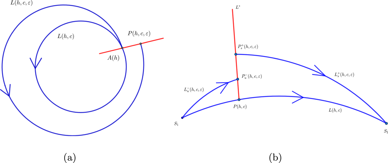
Poincaré map $d_i$ ($i=1,2$) is a powerful tool to study the bifurcation of homoclinic or heteroclinic orbits (e.g., see [Reference Han19, Reference Wen34, Reference Wiggins35, Reference Zhu, Wu, Yu and Shen45]).

1. Case a. It is defined by [see figure 5(a)]

   \[ d_1:A(h)\longrightarrow P(h,c,\varepsilon), \]
   and
   \begin{align*} d_1(h,c,\varepsilon)& =\displaystyle \int_{A(h)}^{P(h,c,\varepsilon)}\,{\rm d}H\\ & =\displaystyle \int_{-\infty}^{+\infty}\left(\frac{\partial H}{\partial x}\frac{{\rm d}x}{{\rm d}t}+\frac{\partial H}{\partial y}\frac{{\rm d}y}{{\rm d}t}\right)\mid_{L_{(h,c,\varepsilon)}}\,{\rm d}t, \end{align*}
   where $A(h)$ is the initial point and $P(h,c,\varepsilon )$ is the mapping point. $L(h,c,\varepsilon )$ and $L(h,c)$ are the perturbed and unperturbed orbits, respectively. We have $\lim \limits _{\varepsilon \rightarrow 0 }L(h,c,\varepsilon )=L(h,c)$. And $d_1(h,c,\varepsilon )$ can be Taylor expanded in $\varepsilon$, one has
   \[ d_1(h,c,\varepsilon)=\varepsilon M_{\text{hom}}(h,c)+O(\varepsilon^2). \]

2. Case b. A heteroclinic orbit $L(h,c)$ connecting two saddle points $S_1$ and $S_2$. Then, $L^+_{s}(h,c,\varepsilon )$ and $L^{-}_{u}(h,c,\varepsilon )$ represent the stable and unstable manifolds of perturbed heteroclinic orbit $L(h,c,\varepsilon )$. Taking a point $P(h,c)\in L(h,c)$, we let $L^*$ be a segment normal of $L(h,c)$ at point $P(h,c)$. For $0<\varepsilon \ll 1$, we assume that $L^+_{s}(h,c,\varepsilon )$ and $L^{-}_{u}(h,c,\varepsilon )$ intersect the normal line $L^*$ transversally at points $P^+_{s}(h,c,\varepsilon )$ and $P^{-}_{u}(h,c,\varepsilon )$ [see figure 5(b)].

Figure 5.

Poincaré map. (a) The type of periodic or homoclinic orbits (b) The type of heteroclinic orbits.

Let

\[ d_2(h,c,\varepsilon)={-}\overrightarrow{n}\cdot\overrightarrow{P^+_{s}P^{-}_{u}}, \]

where $\overrightarrow {n}=\frac {(H_z(P(h,c)),H_y(P(h,c)))}{\mid (H_y(P(h,c)),-H_z(P(h,c)))\mid }$. And $d_2(h,c,\varepsilon )$ can be Taylor expanded in $\varepsilon$, we have

\[ d_2(h,c,\varepsilon)=\varepsilon \cdot A\cdot M_{\text{het}}(h,c)+O(\varepsilon^2), \]

where $A$ is a constant.

Usually, $d_i(h,c,\varepsilon )$ ($i=1,2$) is used to measure the distance between perturbed stable and unstable manifolds. Then, we say that $M_{\text {hom}}(h,c)$ or $M_{\text {het}}(h,c)$ is the so called ‘first-order’ Melnikov integral.

In this paper, ‘first-order’ Melnikov integral is employed to detect the persistence of the homoclinic and heteroclinic orbits under small perturbation, respectively. Consequently, the existence of solitary and kink wave solutions are proved under small perturbation.

Firstly, the homoclinic Melnikov function of system (3.16) is defined by

(5.3)\begin{equation} M_{\text{hom}}(c,{\kappa})=\oint_{\Gamma({\kappa})}\left(\frac{9}{2}z^2-9z+3+\frac{1}{c^2}\right)y^2\,{\rm d}\zeta=\frac{1}{c^2}I({\kappa})+J({\kappa}), \end{equation}

where $I({\kappa })=\oint _{\Gamma ({\kappa })}y^2\,{\rm d}\zeta$ and $J({\kappa })=\oint _{\Gamma ({\kappa })}\left (\frac {9}{2}z^2-9z+3\right )y^2\,{\rm d}\zeta$.

Proof. Obviously, we know that $I({\kappa })=\displaystyle \oint _{\Gamma ({\kappa })}y^2\,{\rm d}\zeta >0$. Because $J({\kappa })$ integrates along the homoclinic orbit $\Gamma ({\kappa })$, then

(5.4)\begin{equation} y''=\left(\frac{9}{2}z^2-9z+3\right)z'=\left(\frac{9}{2}z^2-9z+3\right)y, \end{equation}

which yields

(5.5)\begin{equation} {\rm d}y'=\left(\frac{9}{2}z^2-9z+3\right)z'\,{\rm d}\zeta=\left(\frac{9}{2}z^2-9z+3\right)y\,{\rm d}\zeta. \end{equation}

By integration of parts, it is not difficult to have

(5.6)\begin{align} J({\kappa})& =\oint_{\Gamma({\kappa})}(\frac{9}{2}z^2-9z+3)y^2\,{\rm d}\zeta=\displaystyle\oint_{\Gamma({\kappa})}y\,{\rm d}y'\nonumber\\ & ={-}\int_\mathbb{R}(y')^2\,{\rm d}\zeta<0. \end{align}

Hence, $-\frac {I({\kappa })}{J({\kappa })}>0$, there exists a single positive root $c=c({\kappa })$ of $M_{\text {hom}}(c,{\kappa })=0$ that

(5.7)\begin{equation} c({\kappa})=\sqrt{-\frac{I({\kappa})}{J({\kappa})}}. \end{equation}

On the other hand, it follows from (5.3) that

(5.8)\begin{equation} \frac{\partial M_{\text{hom}}(c,{\kappa})}{\partial c}\mid_{c=c({\kappa})}={-}2\frac{1}{c^3}I({\kappa})={-}2J({\kappa})\sqrt{-\frac{J({\kappa})}{I({\kappa})}}>0. \end{equation}

The proof is completed.

In fact, the analytical expressions of $I({\kappa })$ and $J({\kappa })$ can be computed by dividing them into two cases.

Case (I): $1+\frac {\sqrt 3}{3}<{\kappa }<2$.

Firstly, since $I{({\kappa })}$ and $J{({\kappa })}$ are integrated over a closed curve, and the time variable $\zeta$ can be represented by the state variable $z$ on homoclinic orbit. Thus, by (4.5), we have

(5.9)\begin{align} I({\kappa})& =\displaystyle\oint_{\Gamma({\kappa})}y^2\,{\rm d}\zeta=\oint_{\Gamma({\kappa})}y\,{\rm d}z\nonumber\\ & =2 \displaystyle\int_{z_+}^{\kappa}\sqrt{\frac{3}{4}z^4-3z^3+3z^2-(3{\kappa}^3-9{\kappa}^2+6{\kappa})z+\frac{9}{4}{\kappa}^4-6{\kappa}^3+3{\kappa}^2}\,{\rm d}z\nonumber\\ & =2 \displaystyle\int_{z_+}^{\kappa}\sqrt{\frac{3}{4}(z-{\kappa})^2(z-z_+)(z-z_-)}\,{\rm d}z\nonumber\\ & =\sqrt{3} \left[\displaystyle\int_{z_+}^{\kappa}{\kappa}\sqrt{(z-z_+)(z-z_-)}\,{\rm d}z-\displaystyle\int_{z_+}^{\kappa}z\sqrt{(z-z_+)(z-z_-)}\,{\rm d}z \right]\nonumber\\ & = \sqrt{3} \left[{\kappa}I_1({\kappa})-I_2({\kappa}) \right], \end{align}

where $I_1({\kappa })=\int _{z_+}^{\kappa }\sqrt {(z-z_+)(z-z_-)}\,{\rm d}z$ and $I_2({\kappa })=\int _{z_+}^{\kappa }z\sqrt {(z-z_+)(z-z_-)}\,{\rm d}z$.

Note that the formulas 2.261, 2.262 (1) and 2.262 (2) in handbook [Reference Gradshteyn and Ryzhik17] read:

(5.10)\begin{equation} \begin{aligned} \int \frac{{\rm d}x}{\sqrt R} & = \frac{1}{\sqrt{c_1}}\text{ln}(2\sqrt{c_1R}+2c_1x+b),\quad (c_1>0, \ 2c_1x+b>\sqrt{-\Delta}, \ \Delta<0),\\ \int\sqrt R\,{\rm d}x & = \frac{(2c_1x+b)\sqrt R}{4c_1}+\frac{\Delta}{8c_1}\displaystyle \int \frac{{\rm d}x}{\sqrt R},\\ \int x\sqrt R\,{\rm d}x & = \frac{\sqrt{R^3}}{3c_1}-\frac{(2c_1x+b)b\sqrt R}{8c_1^2}-\frac{b\Delta}{16c_1^2}\int \frac{{\rm d}x}{\sqrt R}, \end{aligned} \end{equation}

where $R=a+bx+c_1x^2$ and $\Delta =4ac_1-b^2$. Combining (5.9) and (5.10), it follows that

(5.11)\begin{align} I({\kappa})& =\frac{\sqrt3}{3}\left[6\text{ln}2{\kappa}^3+6{\kappa}^3\text{ln}\left(\sqrt{6{\kappa}^2-12{\kappa}+4}+2{\kappa}-2\right)-18\text{ln}2{\kappa}^2\right.\nonumber\\ & \quad-18{\kappa}^2\text{ln}\left(\sqrt{6{\kappa}^2-12{\kappa}+4}+2{\kappa}-2\right)+12\text{ln}2{\kappa}\nonumber\\ & \quad\left.+12{\kappa}\text{ln}\left(\sqrt{6{\kappa}^2-12{\kappa}+4}+2{\kappa}-2\right)+2\sqrt{6{\kappa}^2-12{\kappa}+4}\right]\nonumber\\ & \quad-\sqrt3 {\kappa}\left[{\kappa}^2\text{ln}(2{\kappa}-{\kappa}^2)+3\text{ln}2{\kappa}^2-3{\kappa}\text{ln}(2{\kappa}-{\kappa}^2)-9\text{ln}2{\kappa}\right.\nonumber\\ & \quad\left.+2\text{ln}(2{\kappa}-{\kappa}^2)+6\text{ln}2\right]. \end{align}

Secondly,

(5.12)\begin{equation} \begin{aligned} J({\kappa}) & =\oint_{\Gamma({\kappa})}\left(\frac{9}{2}z^2-9z+3\right)y^2\,{\rm d}\zeta =\oint_{\Gamma({\kappa})}\left(\frac{9}{2}z^2-9z+3\right)y\,{\rm d}z\\ & =2 \int_{z_+}^{\kappa}\left(\frac{9}{2}z^2-9z+3\right)\\ & \qquad\sqrt{\frac{3}{4}z^4-3z^3+3z^2-(3{\kappa}^3-9{\kappa}^2+6{\kappa})z+\frac{9}{4}{\kappa}^4-6{\kappa}^3+3{\kappa}^2}\,{\rm d}z\\ & =\sqrt{3} \int_{z_+}^{\kappa}\left(\frac{9}{2}z^2-9z+3\right)\sqrt{({\kappa}-z)^2(z-z_+)(z-z_-)}\,{\rm d}z\\ & =\sqrt{3}\int_{z_+}^{\kappa}\left[-\frac{9}{2}z^3+\left(\frac{9}{2}{\kappa}+9\right)z^2-(9{\kappa}+3)z+3{\kappa}\right]\sqrt{(z-z_+)(z-z_-)}\,{\rm d}z \\ & = \sqrt{3} \left[-\frac{9}{2}J_1({\kappa})+\left(\frac{9}{2}{\kappa}+9\right)J_2({\kappa})-(9{\kappa}+3)I_2({\kappa})+3{\kappa}I_1({\kappa}) \right], \end{aligned} \end{equation}

where $J_1({\kappa })=\displaystyle \int _{z_+}^{\kappa }z^3\sqrt {(z-z_+)(z-z_-)}\,{\rm d}z$, $J_2({\kappa })=\displaystyle \int _{z_+}^{\kappa }z^2\sqrt {(z-z_+)(z-z_-)}\,{\rm d}z$.

Similarly, by the formulas 2.262 (3) and 2.262 (4) in [Reference Gradshteyn and Ryzhik17], they are expressed by:

(5.13)\begin{equation} \begin{aligned} \int x^2\sqrt R\,{\rm d}x & = \left(\frac{x}{4c_1}-\frac{5b}{24c_1^2}\right)\sqrt {R^3}+\left(\frac{5b^2}{16c_1^2}-\frac{a}{4c_1}\right)\frac{(2c_1x+b)\sqrt R}{4c_1}\\ & \quad +\left(\frac{5b^2}{16c_1^2}-\frac{a}{4c_1}\right)\frac{\Delta}{8c_1}\displaystyle \int \frac{{\rm d}x}{\sqrt R},\\ \int x^3\sqrt R\,{\rm d}x & = \left(\frac{x^2}{5c_1}-\frac{7bx}{40c_1^2}+\frac{7b^2}{48c_1^3}-\frac{2a}{15c_1^2}\right)\sqrt {R^3} -\left(\frac{7b^3}{32c_1^3}-\frac{3ab}{8c_1^2}\right)\frac{(2c_1x+b)\sqrt R}{4c_1}\\ & \quad- \left(\frac{7b^3}{32c_1^3}-\frac{3ab}{8c_1^2}\right)\frac{\Delta}{8c_1}\int \frac{{\rm d}x}{\sqrt R}. \end{aligned} \end{equation}

Using (5.10), (5.12) and (5.13), we have

(5.14)\begin{align} J({\kappa})& ={-}\frac{\sqrt3}{5} \left[27{\kappa}^4 \sqrt{6{\kappa}^2-12{\kappa}+4}+15 {\kappa}^3\text{ln}(2{\kappa}-{\kappa}^2)-198{\kappa}^3\sqrt{6{\kappa}^2-12{\kappa}+4}\right.\nonumber\\ & \quad-30{\kappa}^3\text{ln}\left(\sqrt{6{\kappa}^2-12{\kappa}+4}+2{\kappa}-2\right)+15\text{ln}2{\kappa}^3-45{\kappa}^2\text{ln}(2{\kappa}-{\kappa}^2) \nonumber\\ & \quad+90{\kappa}^2\text{ln}\left(\sqrt{6{\kappa}^2-12{\kappa}+4}+2{\kappa}-2\right)+30\sqrt2{\kappa}\sqrt{(3{\kappa}^2-6{\kappa}+2)^3}\nonumber\\ & \quad+294{\kappa}^2\sqrt{6{\kappa}^2-12{\kappa}+4}-45\text{ln}2{\kappa}^2+30{\kappa}\text{ln}(2{\kappa}-{\kappa}^2)\nonumber\\ & \quad-60{\kappa}\text{ln}\left(\sqrt{6{\kappa}^2-12{\kappa}+4}+2{\kappa}-2\right)+10\sqrt2\sqrt{(3{\kappa}^2-6{\kappa}+2)^3}\nonumber\\ & \quad\left.-72{\kappa}\sqrt{6{\kappa}^2-12{\kappa}+4}+30\text{ln}2{\kappa}-18\sqrt{6{\kappa}^2-12{\kappa}+4}\right]. \end{align}

Case (II): $0<{\kappa }<1-\frac {\sqrt 3}{3}$.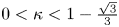

Same calculation method as case (I), we obtain

(5.15)\begin{align} I({\kappa})& =\oint_{\Gamma({\kappa})}y^2\,{\rm d}\zeta=\oint_{\Gamma({\kappa})}y\,{\rm d}z=2 \int_{z_-}^{\kappa}\cdots\,{\rm d}z\nonumber\\ & =\frac{\sqrt3}{3}\left[6\text{ln}2{\kappa}^3+6{\kappa}^3\text{ln}\left(\sqrt{6{\kappa}^2-12{\kappa}+4}+2{\kappa}-2\right)-18\text{ln}2{\kappa}^2\right.\nonumber\\ & \quad-18{\kappa}^2\text{ln}\left(\sqrt{6{\kappa}^2-12{\kappa}+4}+2{\kappa}-2\right)+12\text{ln}2{\kappa}\nonumber\\ & \quad\left.+12{\kappa}\text{ln}\left(\sqrt{6{\kappa}^2-12{\kappa}+4}+2{\kappa}-2\right)+2\sqrt{6{\kappa}^2-12{\kappa}+4}\right]\nonumber\\ & \quad-\sqrt3 {\kappa}\left[2{\kappa}^2\text{ln}\left(-\sqrt{2{\kappa}-{\kappa}^2}\right)+3\text{ln}2{\kappa}^2-6{\kappa}\text{ln}\left(-\sqrt{2{\kappa}-{\kappa}^2}\right)-9\text{ln}2{\kappa}\right.\nonumber\\ & \quad\left.+4\text{ln}\left(-\sqrt{2{\kappa}-{\kappa}^2}\right)+6\text{ln}2\right], \end{align}

and

(5.16)\begin{align} J({\kappa})& =\oint_{\Gamma({\kappa})}\left(\frac{9}{2}z^2-9z+3\right)y^2\,{\rm d}\zeta=\oint_{\Gamma({\kappa})}\left(\frac{9}{2}z^2-9z+3\right)y\,{\rm d}z=2 \int_{z_-}^{\kappa}\cdots {\rm d}z\nonumber\\ & ={-}\frac{\sqrt3}{5} \left[27{\kappa}^4 \sqrt{6{\kappa}^2-12{\kappa}+4}+30 {\kappa}^3\text{ln}\left(-\sqrt{2{\kappa}-{\kappa}^2}\right)+60{\kappa}\text{ln}\left(-\sqrt{2{\kappa}-{\kappa}^2}\right)\right.\nonumber\\ & \quad-30{\kappa}^3\text{ln}\left(\sqrt{6{\kappa}^2-12{\kappa}+4}+2{\kappa}-2\right)+15\text{ln}2{\kappa}^3-90{\kappa}^2\text{ln}\left(-\sqrt{2{\kappa}-{\kappa}^2}\right) \nonumber\\ & \quad+90{\kappa}^2\text{ln}\left(\sqrt{6{\kappa}^2-12{\kappa}+4}+2{\kappa}-2\right)+30\sqrt2{\kappa}\sqrt{(3{\kappa}^2-6{\kappa}+2)^3}\nonumber\\ & \quad+294{\kappa}^2\sqrt{6{\kappa}^2-12{\kappa}+4}-45\text{ln}2{\kappa}^2-198{\kappa}^3\sqrt{6{\kappa}^2-12{\kappa}+4}\nonumber\\ & \quad-60{\kappa}\text{ln}\left(\sqrt{6{\kappa}^2-12{\kappa}+4}+2{\kappa}-2\right)+10\sqrt2\sqrt{(3{\kappa}^2-6{\kappa}+2)^3}\nonumber\\ & \quad\left.-72{\kappa}\sqrt{6{\kappa}^2-12{\kappa}+4}+30\text{ln}2{\kappa}-18\sqrt{6{\kappa}^2-12{\kappa}+4}\right]. \end{align}

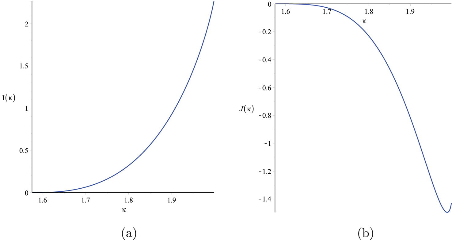
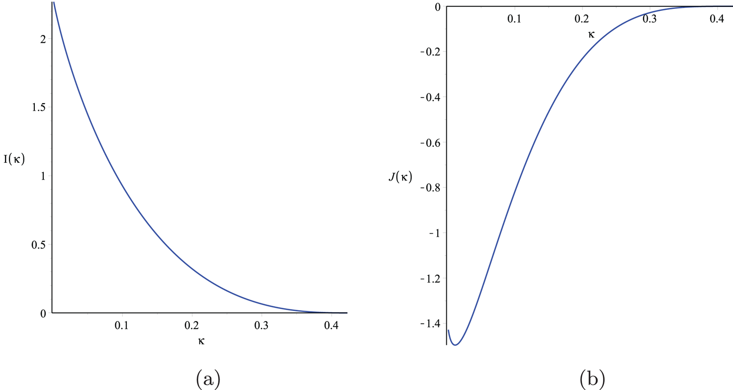
We plot the algebraic curve of $I({\kappa })$ with respect to ${\kappa }$ and $J({\kappa })$ with respect to ${\kappa }$, respectively. (see figures 6 and 7)

Figure 6.

The algebraic curves of $I({\kappa })$ and $J({\kappa })$ with respect to ${\kappa }$ for $1+\frac {\sqrt 3}{3}<{\kappa }<2$. (a) (${\kappa }$, $I(\kappa )$) (b) (${\kappa }$, $J(\kappa )$).

Figure 7.

The algebraic curves of $I({\kappa })$ and $J({\kappa })$ with respect to ${\kappa }$ for $0<{\kappa }<1-\frac {\sqrt 3}{3}$. (a) (${\kappa }$, $I(\kappa )$) (b) (${\kappa }$, $J(\kappa )$).

We can see that $I({\kappa })>0$ and $J({\kappa })<0$ for $1+\frac {\sqrt 3}{3}<{\kappa }<2$ in figure 6, $I({\kappa })>0$ and $J({\kappa })<0$ for $0<{\kappa }<1-\frac {\sqrt 3}{3}$ in figure 7. It is shown that a good agreement with the proof of lemma 5.4.

Hence, we substitute (5.11) and (5.14) into (5.3), and the expression of the homoclinic Melnikov function of system (3.16) for $1+\frac {\sqrt 3}{3}<{\kappa }<2$ can be rewritten as

(5.17)\begin{align} & M_{\text{hom}}(c,{\kappa})\Big|_{\kappa\in\left(1+\frac{\sqrt3}{3},2\right)}\nonumber\\ & =\frac{1}{c^2}\frac{\sqrt3}{3}\left[6\text{ln}2{\kappa}^3+6{\kappa}^3\text{ln}\left(\sqrt{6{\kappa}^2-12{\kappa}+4}+2{\kappa}-2\right)-18\text{ln}2{\kappa}^2\right.\nonumber\\ & \quad-18{\kappa}^2\text{ln}\left(\sqrt{6{\kappa}^2-12{\kappa}+4}+2{\kappa}-2\right)+12\text{ln}2{\kappa}\nonumber\\ & \quad\left.+12{\kappa}\text{ln}\left(\sqrt{6{\kappa}^2-12{\kappa}+4}+2{\kappa}-2\right)+2\sqrt{6{\kappa}^2-12{\kappa}+4}\right]\nonumber\\ & \quad-\frac{1}{c^2}\sqrt3 {\kappa}\left[{\kappa}^2\text{ln}(2{\kappa}-{\kappa}^2)+3\text{ln}2{\kappa}^2-3{\kappa}\text{ln}(2{\kappa}-{\kappa}^2)-9\text{ln}2{\kappa}\right.\nonumber\\ & \quad\left.+2\text{ln}(2{\kappa}-{\kappa}^2)+6\text{ln}2\right]-\frac{\sqrt3}{5} \left[27{\kappa}^4 \sqrt{6{\kappa}^2-12{\kappa}+4}\right.\nonumber\\ & \quad+15 {\kappa}^3\text{ln}(2{\kappa}-{\kappa}^2)-198{\kappa}^3\sqrt{6{\kappa}^2-12{\kappa}+4}\nonumber\\ & \quad-30{\kappa}^3\text{ln}\left(\sqrt{6{\kappa}^2-12{\kappa}+4}+2{\kappa}-2\right)+15\text{ln}2{\kappa}^3-45{\kappa}^2\text{ln}(2{\kappa}-{\kappa}^2) \nonumber\\ & \quad+90{\kappa}^2\text{ln}\left(\sqrt{6{\kappa}^2-12{\kappa}+4}+2{\kappa}-2\right)+30\sqrt2{\kappa}\sqrt{(3{\kappa}^2-6{\kappa}+2)^3}\nonumber\\ & \quad+294{\kappa}^2\sqrt{6{\kappa}^2-12{\kappa}+4}-45\text{ln}2{\kappa}^2+30{\kappa}\text{ln}(2{\kappa}-{\kappa}^2)\nonumber\\ & \quad-60{\kappa}\text{ln}\left(\sqrt{6{\kappa}^2-12{\kappa}+4}+2{\kappa}-2\right)+10\sqrt2\sqrt{(3{\kappa}^2-6{\kappa}+2)^3}\nonumber\\ & \quad\left.-72{\kappa}\sqrt{6{\kappa}^2-12{\kappa}+4}+30\text{ln}2{\kappa}-18\sqrt{6{\kappa}^2-12{\kappa}+4}\right]. \end{align}

It is easy to verify that for $\kappa \in \left (1+\frac {\sqrt 3}{3},2\right )$, there is $c=c_1(\kappa )$ such that $M_{\text {hom}}(c,{\kappa })\Big |_{\kappa \in \left (1+\frac {\sqrt 3}{3},2\right )}=0$.

Similarly, the expression of the homoclinic Melnikov function of system (3.16) for $0<{\kappa }<1-\frac {\sqrt 3}{3}$ is

(5.18)\begin{align} & M_{\text{hom}}(c,{\kappa})\Big|_{\kappa\in\left(0,1-\frac{\sqrt3}{3}\right)}\nonumber\\ & =\frac{1}{c^2}\frac{\sqrt3}{3}\left[6\text{ln}2{\kappa}^3+6{\kappa}^3\text{ln}\left(\sqrt{6{\kappa}^2-12{\kappa}+4}+2{\kappa}-2\right)-18\text{ln}2{\kappa}^2\right.\nonumber\\ & \quad-18{\kappa}^2\text{ln}\left(\sqrt{6{\kappa}^2-12{\kappa}+4}+2{\kappa}-2\right)+12\text{ln}2{\kappa}\nonumber\\ & \quad\left.+12{\kappa}\text{ln}\left(\sqrt{6{\kappa}^2-12{\kappa}+4}+2{\kappa}-2\right)+2\sqrt{6{\kappa}^2-12{\kappa}+4}\right]\nonumber\\ & \quad-\frac{1}{c^2}\sqrt3 {\kappa}\left[2{\kappa}^2\text{ln}\left(-\sqrt{2{\kappa}-{\kappa}^2}\right)+3\text{ln}2{\kappa}^2-6{\kappa}\text{ln}\left(-\sqrt{2{\kappa}-{\kappa}^2}\right)-9\text{ln}2{\kappa}\right.\nonumber\\ & \quad\left.+4\text{ln}\left(-\sqrt{2{\kappa}-{\kappa}^2}\right)+6\text{ln}2\right]-\frac{\sqrt3}{5} \left[27{\kappa}^4 \sqrt{6{\kappa}^2-12{\kappa}+4}\right.\nonumber\\ & \quad+30 {\kappa}^3\text{ln}\left(-\sqrt{2{\kappa}-{\kappa}^2}\right)+60{\kappa}\text{ln}\left(-\sqrt{2{\kappa}-{\kappa}^2}\right)+15\text{ln}2{\kappa}^3\nonumber\\ & \quad-30{\kappa}^3\text{ln}\left(\sqrt{6{\kappa}^2-12{\kappa}+4}+2{\kappa}-2\right)-90{\kappa}^2\text{ln}\left(-\sqrt{2{\kappa}-{\kappa}^2}\right) \nonumber\\ & \quad+90{\kappa}^2\text{ln}\left(\sqrt{6{\kappa}^2-12{\kappa}+4}+2{\kappa}-2\right)+30\sqrt2{\kappa}\sqrt{(3{\kappa}^2-6{\kappa}+2)^3}\nonumber\\ & \quad+294{\kappa}^2\sqrt{6{\kappa}^2-12{\kappa}+4}-45\text{ln}2{\kappa}^2-198{\kappa}^3\sqrt{6{\kappa}^2-12{\kappa}+4}\nonumber\\ & \quad-60{\kappa}\text{ln}\left(\sqrt{6{\kappa}^2-12{\kappa}+4}+2{\kappa}-2\right)+10\sqrt2\sqrt{(3{\kappa}^2-6{\kappa}+2)^3}\nonumber\\ & \quad\left.-72{\kappa}\sqrt{6{\kappa}^2-12{\kappa}+4}+30\text{ln}2{\kappa}-18\sqrt{6{\kappa}^2-12{\kappa}+4}\ \right]. \end{align}

It is easy to verify that for $\kappa \in \left (0,1-\frac {\sqrt 3}{3}\right )$, there is $c=c_2(\kappa )$ such that $M_{\text {hom}}(c,{\kappa })\Big |_{\kappa \in \left (0,1-\frac {\sqrt 3}{3}\right )}=0$.

Secondly, the Melnikov method is also employed to detect the existence of kink (anti-kink) wave solutions under small perturbation. The heteroclinic Melnikov function of system (3.16) is defined as follows:

(5.19)\begin{align} M_{\text{het}}(c,\kappa)& =\int_{\Upsilon(\kappa)}\left(\frac{9}{2}z^2-9z+3+\frac{1}{c^2}\right)y^2\,{\rm d}\zeta\nonumber\\ & =\displaystyle\int_{-\infty}^{+\infty}\left(\frac{9}{2}z^2-9z+3+\frac{1}{c^2}\right)y^2\,{\rm d}\zeta\nonumber\\ & =\int_{0}^{2}\left(\frac{9}{2}z^2-9z+3+\frac{1}{c^2}\right)y\,{\rm d}z\nonumber\\ & =\frac{\sqrt3}{2}\int_{0}^{2}\left(\frac{9}{2}z^2-9z+3+\frac{1}{c^2}\right)z(2-z)\,{\rm d}z={-}\frac{2\sqrt3(3c^2-5)}{15c^2}. \end{align}

Proof. Clearly, it directly follows form (5.19) that $M_{\text {het}}(c,\kappa )=0$ has a positive root $c^\ast =\frac {\sqrt {15}}{3}$. Meanwhile,

\[ \frac{\partial M_{\text{het}}}{\partial c}={-}\frac{4\sqrt{3}}{5c}+\frac{4\sqrt{3}(3c^2-5)}{15c^3}, \]

and

\[ \frac{\partial M_{\text{het}}}{\partial c}\mid_{c=c^\ast}={-}\frac{12\sqrt{5}}{25}\neq0. \]

6. Numerical analysis

Numerical simulations are employed to confirm the theoretical results derived in previous sections. Here, maple software 18.0 is used.

Firstly, we simulate the existence of solitary wave solution of perturbed $(1+1)$-dimensional DLWE (1.3). Let ${\kappa }=1.7$ and $\epsilon =0.01$. By (5.11) and (5.14), we obtain $I(1.7)\approx 0.0648882124$ and $J(1.7)\approx -0.02790800120$ such that $c(1.7)=\sqrt {-\frac {I(1.7)}{J(1.7)}}\approx 1.524819859$. Then, according to theorem 5.1, we take $c=c(1.7)$ and let the initial value be $(z(0),y(0))=(z_+,0)=(1.309950494,0)$ (red point) which the homoclinic orbit would pass through. The phase portraits $(z,y)$ and time history curves $(\zeta,z)$ of system (3.16) are plotted in figure 8.

Figure 8.

(a) Phase portraits with $c=c(1.7)$, (b) Time history curves of $(\zeta,z)$ for system (3.16) for $\epsilon =0.01$, ${\kappa }=1.7$ and initial value $(z(0),y(0))=(z_+,0)=(1.309950494,0)$. (a) $c=c(1.7)$ (b) $(\zeta,z)$.

One can see that the homoclinic orbit and dark solitary wave solution of system (3.16) still persist after a small singular perturbation.

Secondly, set ${\kappa }=0.3$ and $\epsilon =0.01$. By (5.15) and (5.16), we have $I(0.3)\approx 0.0648882229$ and $J(0.3)\approx -0.02790784012$ such that $c(0.3)=\sqrt {-\frac {I(0.3)}{J(0.3)}}\approx 1.524824377$. Taking $c=c(0.3)$ and initial value to be $(z(0),y(0))=(z_-,0)=(0.690049506,0)$ (red point) which the homoclinic orbit would pass through. The phase portraits $(z,y)$ and time history curves $(\zeta,z)$ of system (3.16) are plotted in figure 9.

Figure 9.

(a) Phase portraits with $c=c(0.3)$, (b) Time history curves of $(\zeta,z)$ for system (3.16) for $\epsilon =0.01$, ${\kappa }=0.3$ and initial value $(z(0),y(0))=(z_-,0)=(0.690049506,0)$. (a) $c=c(0.3)$ (b) $(\zeta,z)$.

We see that the homoclinic orbit and bright solitary wave solution of system (3.16) still exist after a small singular perturbation which verifies the theorem 5.1(i) and (ii).

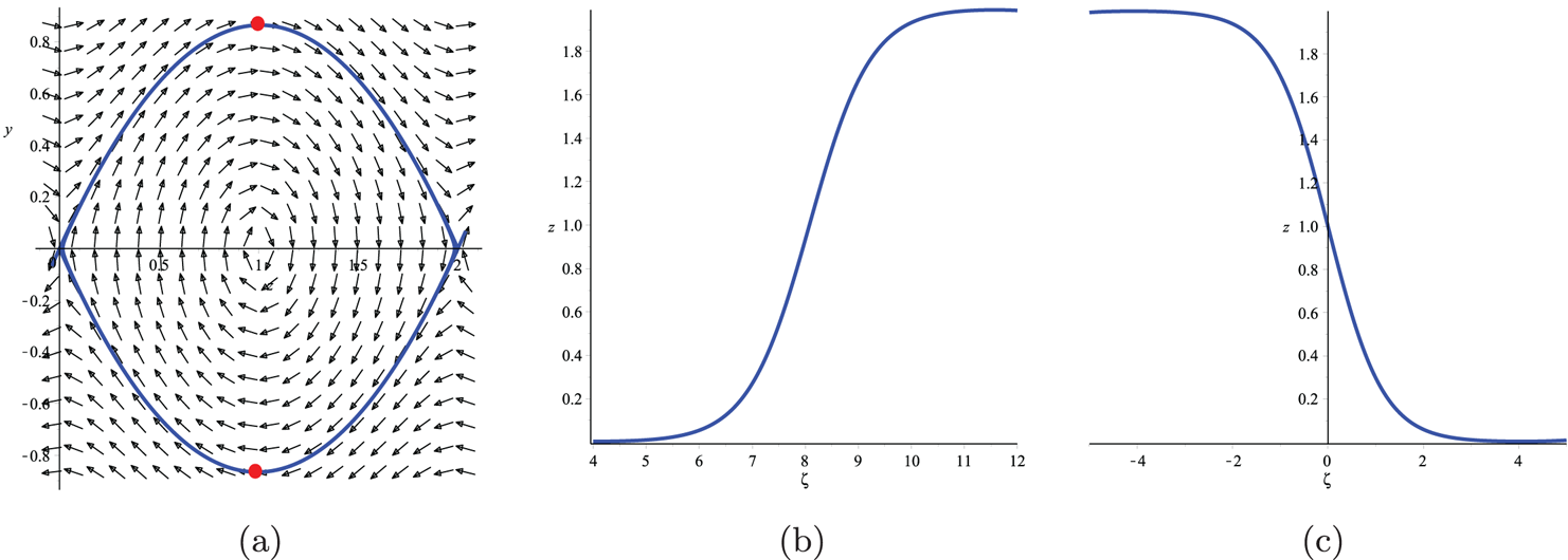
Next, let us to see the existence of kink and anti-kink wave solution of system (3.16). Giving $\kappa =0$ or $\kappa =2$, $\epsilon =0.01$ and initial value $(z(0),y(0))=\left (1,\pm \frac {\sqrt 3}{2}\right )$ (red point). We draw the phase portraits of system (3.16) after taking $c=\frac {\sqrt {15}}{3}$ in figure 10. Form the figure 10(a), it is shown that the heteroclinic orbits still persist. Correspondingly, a pair of kink and anti-kink wave solutions exists [see figures 10(b) and (c)], which is consistent with theorem 5.1(iii).

Figure 10.

Phase portraits with $c=\frac {\sqrt {15}}{3}$ for $\epsilon =0.01$, initial value $(z(0),y(0))=\left (1,\pm \frac {\sqrt 3}{2}\right )$. (a) $c=\frac {\sqrt {15}}{3}$ (b) Kink wave (c) Anti-kink wave.