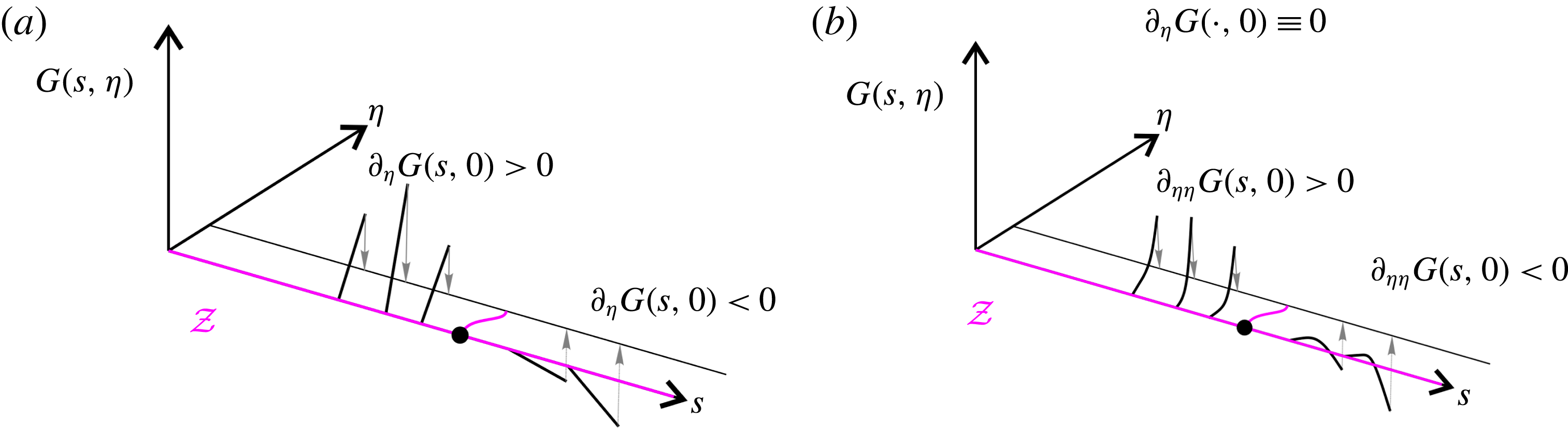
1 Introduction
Fluid flow separation is generally regarded as the detachment of fluid from a no-slip boundary. It is the root cause of several complex flow phenomena, such as vortex formation, wake flow and stall, all of which invariably reduce the performance of engineering flow devices. Following the pioneering work of Prandtl (Reference Prandtl1904) on two-dimensional steady flows, a number of advances have been made towards a better understanding of flow separation. These studies can be divided into two main categories (cf. § 1.1). The first category views separation as the appearance of a singularity in the boundary layer equation (Sears & Telionis Reference Sears and Telionis1971, Reference Sears and Telionis1975). As examples of both separation without such singularities and singularities without separation are known (Liu & Wan Reference Liu and Wan1985), this view practically associates separation with one’s inability to solve the boundary layer equations accurately. The second category views separation as ejection of material from the boundary due to the presence of wall-based non-hyperbolic invariant manifolds in the Lagrangian dynamics (Haller Reference Haller2004). This theory is mathematically exact, and focuses more on longer-term particle dynamics, as opposed to the appearance of separation triggered by the formation of a material spike, i.e. a sharp-shaped set of fluid particles ejected from the wall.
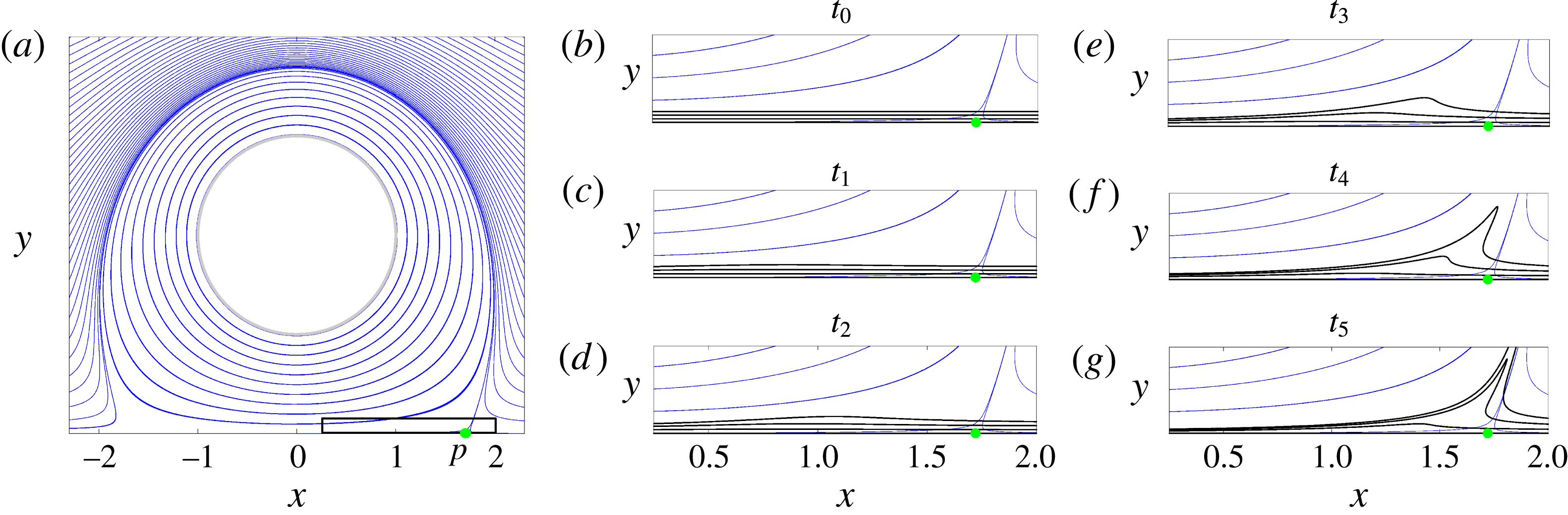
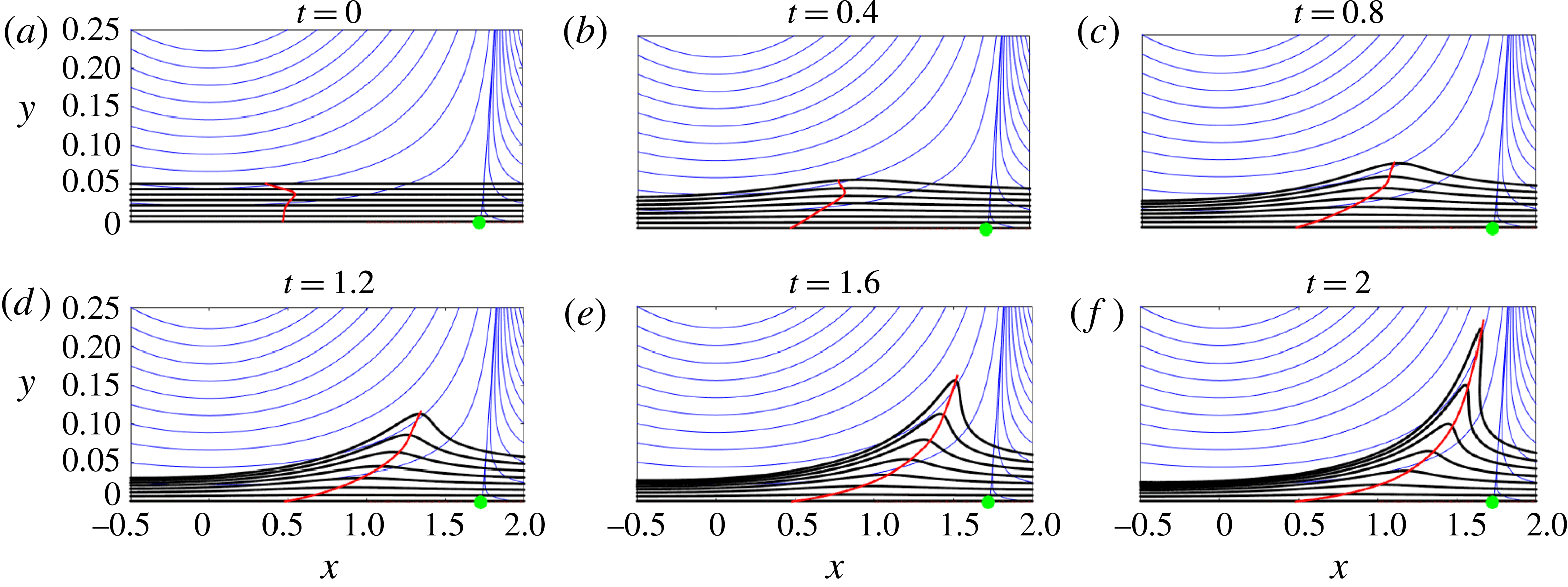
To illustrate the difference between short-term material spikes and longer-term material ejection along unstable manifolds, figure 1 shows the evolution of material lines initially close to the wall in a steady flow analysed in more detail in § 6.1.1. While fluid particles released within the black box in figure 1(a) approach asymptotically the singular streamline (unstable manifold) emanating from the Prandtl point
 $x=p$
(cf. (1.1)), the birth of a material spike takes place at a different upstream location, as shown in figure 1(b–g). A video showing the full time evolution of the material lines is also available online (see supplementary movie 1 at https://doi.org/10.1017/jfm.2018.206).
(a) Streamlines of a steady flow analysed in more detail in § 6.1.1. The green dot represents the Prandtl separation point defined by (1.1). (b–g) Zoom of (a) in the region enclosed by the black rectangle, along with the evolution of the spike visualized through the advection of material lines shown in black. The full evolution of the material spike is shown in supplementary movie 1.

1.1 Prior work on flow separation
Prandtl (Reference Prandtl1904) derived a separation criterion for two-dimensional steady incompressible velocity fields
 $\boldsymbol{f}(x,y)=[u(x,y),v(x,y)]$
that satisfy the no-slip boundary condition
 $\boldsymbol{f}(x,0)=0$
, where
 $x$
is the coordinate parallel to the wall,
 $y$
is normal to the wall and
 $(u,v)$
are the components of the velocity field
 $\boldsymbol{f}$
in the
 $(x,y)$
directions. He showed that streamlines in such a flow separate from the boundary where the skin friction
 $\unicode[STIX]{x1D70F}$
vanishes and admits a negative derivative (cf. figure 1). Thus, according to Prandtl’s criterion, flow separation takes place at a point
 $(p,0)$
if
 $$\begin{eqnarray}\left.\begin{array}{@{}c@{}}\unicode[STIX]{x1D70F}(p)=\unicode[STIX]{x1D708}\unicode[STIX]{x1D70C}u_{y}(p,0)=0,\\ \unicode[STIX]{x1D70F}^{\prime }(p)=\unicode[STIX]{x1D708}\unicode[STIX]{x1D70C}u_{xy}(p,0)<0,\end{array}\right\}\end{eqnarray}$$
where
 $\unicode[STIX]{x1D708}$
and
 $\unicode[STIX]{x1D70C}$
are the kinematic viscosity and the density of the fluid, and
 $(\cdot )_{y}:=(\text{d}/\text{d}y)(\cdot )$
.
While this separation criterion is still often considered to be valid for unsteady flows, several studies have shown this view to be incorrect (Rott Reference Rott1956; Moore Reference Moore1958; Sears & Telionis Reference Sears and Telionis1971). Specifically, Sears & Telionis (Reference Sears and Telionis1975) observed that vanishing wall shear ‘does not denote separation in any meaningful sense in unsteady flow’, and proposed the Moore–Root–Sears (MRS) criterion. This criterion states that in the limit of infinite Reynolds numbers (
 $Re$
), unsteady separation takes place at a point off the boundary where
 $u_{y}$
vanishes and the streamwise velocity equals the velocity of the separation structure. The restriction to
 $Re\rightarrow \infty$
together with the reliance on the a priori unknown velocity of the separation structure, however, makes the MRS principle practically inapplicable (Williams Reference Williams1977; Van Dommelen Reference Van Dommelen1981).
A large number of numerical studies have focused on solving the boundary layer equations, defining the separation point as the location where the solution of these equations becomes singular (Sears & Telionis Reference Sears and Telionis1971, Reference Sears and Telionis1975). Subsequently, by using Lagrangian coordinates, Van Dommelen (Reference Van Dommelen1981) and Van Dommelen & Shen (Reference Van Dommelen and Shen1982) overcame the computational difficulties seen earlier in the Eulerian frame. Analytic results show, however, that separation in the boundary layer equations has no direct connection with velocity singularities (Liu & Wan Reference Liu and Wan1985). Furthermore, these methods are inapplicable to physical two-dimensional Navier–Stokes flows, which do not exhibit singularities. This problem has been partially solved by the triple-deck theory, which models the interaction between the viscous boundary layer and the outer inviscid region (see, e.g., Sychev & Sychev (Reference Sychev and Sychev1998)). The triple-deck theory, however, like the MRS criterion, assumes an infinite Reynolds number (see also the recent reviews by Ruban et al. (Reference Ruban, Araki, Yapalparvi and Gajjar2011) and Cassel & Conlisk (Reference Cassel and Conlisk2014)).
Using dynamical systems theory, Shariff, Pulliam & Ottino (Reference Shariff, Pulliam and Ottino1991) and Yuster & Hackborn (Reference Yuster and Hackborn1997) proposed a rigorous criterion for the existence of a material spike on a no-slip boundary in a near-steady time-periodic incompressible flow. In particular, they defined the separation profile in such a flow as the unstable manifold of a non-hyperbolic fixed point on the wall. Extending this idea, Haller (Reference Haller2004) developed a general theory of separation for a broader class of unsteady flows, defining two types of separation: fixed and moving separation. Fixed separation occurs in flows with a well-defined asymptotic mean (Kilic, Haller & Neishtadt Reference Kilic, Haller and Neishtadt2005), such as periodic and quasiperiodic flows, as well as aperiodic flows with a mean component. In this case, the separation point on the boundary is fixed at a location where the backward-time average of the skin friction vanishes, and the angle of separation is generally time-dependent. In the case of compressible flows, the skin-friction average in this criterion is weighted by a function of the flow density. These results have also been extended to three-dimensional flows (Surana, Grunberg & Haller Reference Surana, Grunberg and Haller2006; Surana et al. Reference Surana, Jacobs, Grunberg and Haller2008).
To define moving separation points, Haller (Reference Haller2004) used finite-time unstable manifold ideas from Haller (Reference Haller2000) which are mathematically rigorous but give non-unique results. In a later contribution, Surana & Haller (Reference Surana and Haller2008) derived an exact separation criterion for slow–fast flows (i.e. unsteady flows where the mean and fluctuating components have different time scales). The separation point then arises at a location where the time-varying mean skin friction vanishes. This criterion, however, relies on a precise extraction of a slow mean-flow component of the velocity field.
Recently, using the theory of Lagrangian coherent structures (LCSs), Miron & Vétel (Reference Miron and Vétel2015) proposed a different approach to moving separation. They defined the separation point as an off-wall Lagrangian saddle-type trajectory whose finite-time unstable manifold acts as the observed separation profile. This separation profile is an attracting LCS (Farazmand & Haller Reference Farazmand and Haller2012) initiated from a set of points satisfying suitable attraction properties. Among all attracting LCSs, they select a particular subset on which the backward finite time Lyapunov exponent (FTLE) achieves a relative maximum within a prescribed neighbourhood. Finally, the separation point along the remaining LCSs is selected as the point where the time-averaged normal repulsion rate is maximal after long enough time.
One may look for truly off-wall separation, but it may not exist. At the same time, not being able to find an on-wall signature of a given separation phenomenon does not imply that it has none. For instance, although commonly thought otherwise (see, e.g., Miron & Vétel (Reference Miron and Vétel2015)), in the classic example of flow separation over a moving boundary, the separation point does have a clear on-wall Eulerian signature in a frame co-moving with the boundary (see Surana & Haller (Reference Surana and Haller2008), figure 7). Therefore, the existence of a truly off-wall separation point in real-life flows has been an unsettled question.
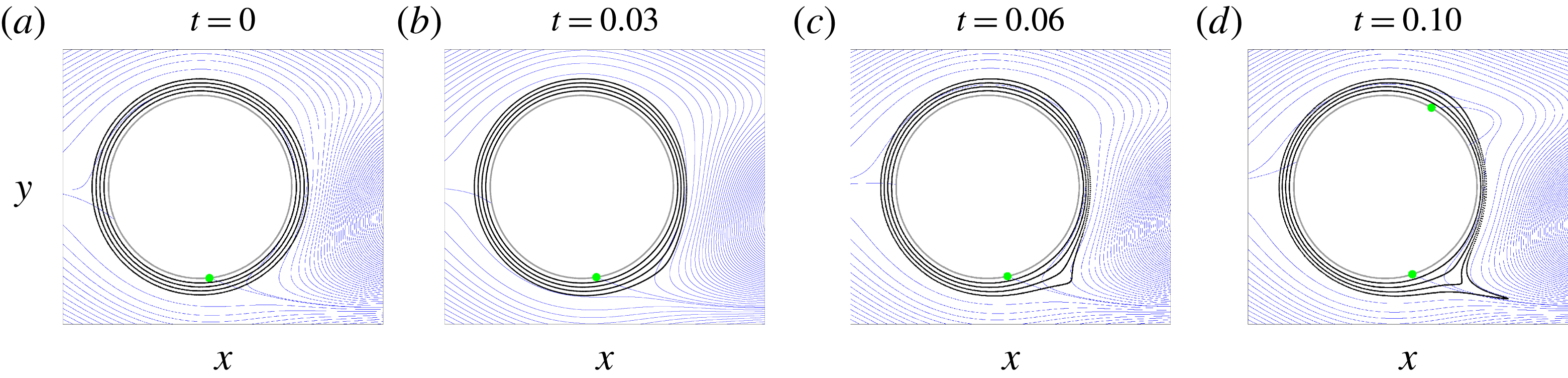
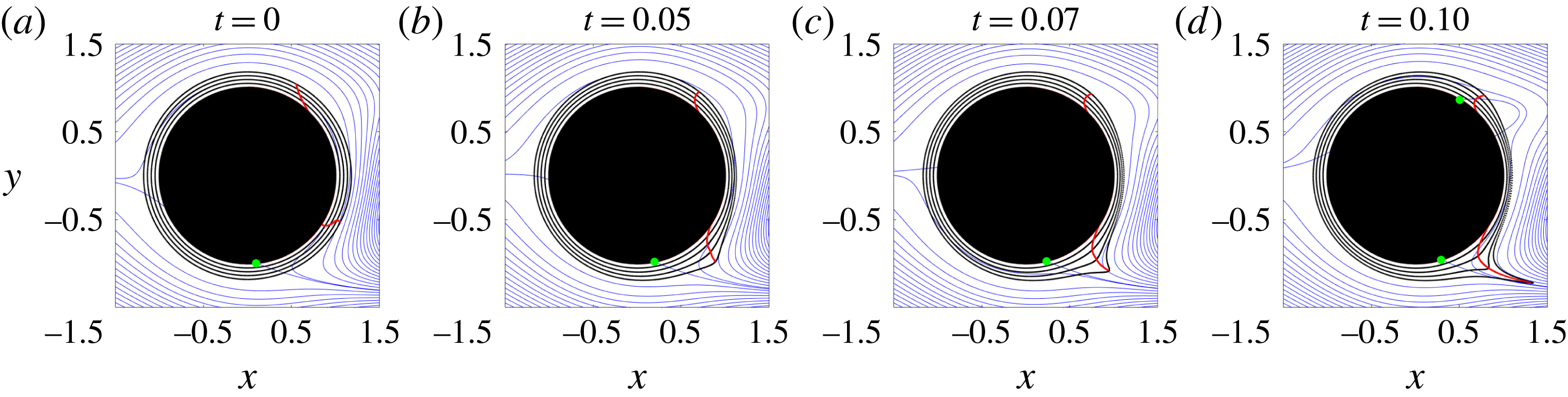
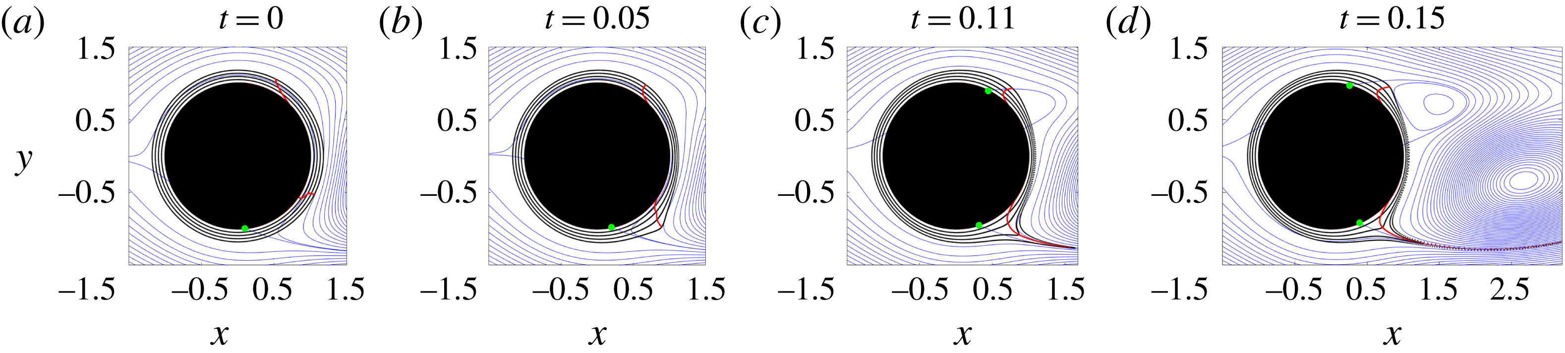
Similarly to figure 1, figure 2 shows the evolution of material lines (black) in the flow past a circular cylinder, analysed in more detail in § 6.3, over the time interval
 $[0,0.1]$
. The instantaneous streamlines and Prandtl separation point are shown in blue and green respectively. Although this flow is time-periodic with period
 $T_{p}\approx 1.1$
, within the finite time interval we used, the flow appears aperiodic. Even over this short time interval, however, one observes a clear spike formation exactly as in the steady flow example of figure 1. This highlights two important facts. First, the spike formation shows a qualitatively similar behaviour in both steady and unsteady flows. Second, and more important, existing criteria would be unable to detect such spike formation over these short time intervals because they are either inapplicable or are designed to capture the long-term (asymptotic) separation profile.
(a) Initial position of material lines (black) in a time-periodic flow analysed in more detail in § 6.3. The instantaneous streamlines and Prandtl separation points (cf. (1.1)) are shown in blue and green respectively. (b–d) Advected images of material lines within the time interval
 $[0,0.1]$
. The full evolution of material lines is available as supplementary movie 2.

From both a phenomenological and a flow-control perspective, one would ideally need a universal definition of the evolving theoretical centrepiece (backbone) of the material spike irrespective of the time dependence, the asymptotic properties and the time scales of the separating flow. Such a definition should be effective also over short time intervals, and ideally admit a rigorous instantaneous limit. In summary, despite significant advances in the long-term phenomenological study of flow separation, a rigorous general theory for the material spike formation universally observed in separation experiments has still been missing.
1.2 Main results
In this paper, we derive a general frame-independent theory of material spike formation over a no-slip boundary in a two-dimensional flow with arbitrary time dependence. Our theory identifies both fixed and moving separation, and is effective also over short time intervals, inaccessible to previous theories.
Our results are based on explicit formulae for the evolution of material line curvature. Material spike formation can then be captured as the emergence of the locus of curvature maxima near the boundary. If such a ridge of the material curvature field emanates from a fixed point on the boundary, we speak of fixed separation. Otherwise, we identify the separation as moving.
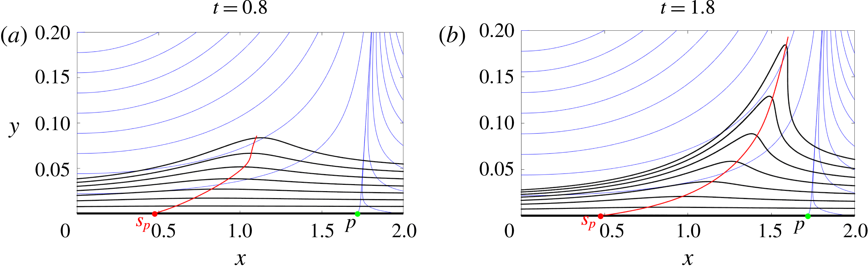
Although in the boundary layer equation community the spike formation has exclusively been associated with unsteady separation (Van Dommelen Reference Van Dommelen1981; Van Dommelen & Shen Reference Van Dommelen and Shen1982), figure 1 shows that the same phenomenon also exists in steady flows, as noted above. Using the flow of figure 1, in figure 3, we show the backbone of the material spike in red, along with the streamlines in blue and the material lines initially parallel to the wall in black. Most importantly, we uncover a previously undocumented spiking point
 $s_{p}$
, at which the backbone of the separation spike connects to the wall. Remarkably, even in steady flows, the spiking point differs from the classic zero-skin-friction point
 $p$
identified by Prandtl.
Backbone of separation (red curve) in a steady flow (cf. § 6.1.1) at two different times, along with the streamlines (blue) and material lines initially parallel to the wall (black). The green dot represents the Prandtl separation point (cf. (1.1)), while the red dot marks the spiking point (cf. table 1) where the backbone connects to the wall.

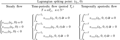
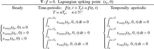
In table 1, we summarize the general formulae that we will derive later for the Lagrangian spiking point in the case of incompressible flows analysed over a time interval
 $[t_{0},t_{0}+T]$
(see § 4 for compressible flows).
Exact criteria for the location of the Lagrangian spiking point on a flat no-slip boundary in the case of an incompressible flow observed over the time interval
 $[t_{0},t_{0}+T]$
.

In § 4, we show that for steady flows and time-periodic flows analysed over a multiple of their period, the spiking point is fixed, as is the classic asymptotic separation point (Prandtl Reference Prandtl1904; Haller Reference Haller2004). The backbone of the separation spike, however, evolves even in steady flows, serving as the theoretical centrepiece of the developing material spike. In contrast, the corresponding asymptotic separation profiles are fixed. Although our main interest is to capture the birth of the material spike, in appendix D.3, we also derive explicit formulae for the asymptotic
 $(T\rightarrow \infty )$
mean location of the spiking point in the case of unsteady velocity fields with a finite mean component such as quasiperiodic velocity fields. These formulae apply to canonical separation problems, such as separation behind a cylinder or a backward facing step, which admit a finite number of dominant frequencies in their Fourier spectra.
The spiking point in table 1 involves higher-order derivatives of the velocity field. These can be computed spectrally in direct numerical simulations, but would be challenging to measure experimentally. In § 4, however, we derive an alternative topological definition of spiking points without higher derivatives. In the case of incompressible flows, our spiking point criteria can also be computed from an approximate velocity field reconstructed from wall-based quantities (cf. appendix F).
Our theory also explains the perception of off-wall separation in unsteady flows, providing conditions under which such a perception is correct. Additionally, in the limit of zero advection time, our Lagrangian definition of the backbone of separation turns into a frame-invariant Eulerian definition. We believe that this objective Eulerian identification of the birth of a separation spike will be useful in active flow-control applications.
This paper is organized as follows. We first develop our theoretical results in §§ 2–4, then we give an algorithmic summary of our Lagrangian and Eulerian backbones of separation in § 5. In § 6, we illustrate our results on several examples, including steady, time-periodic and unsteady analytic velocity fields with flat and curved boundaries, as well as an experimental velocity dataset.
2 Set-up and notation
We consider the two-dimensional non-autonomous dynamical system
 $$\begin{eqnarray}\dot{\boldsymbol{z}}=\boldsymbol{f}(\boldsymbol{z},t),\quad \boldsymbol{f}(\boldsymbol{z},t)=[u(\boldsymbol{z},t),v(\boldsymbol{z},t)]^{\top },\quad \boldsymbol{z}=[x,y]^{\top }\in U\subset \mathbb{R}^{2},\end{eqnarray}$$
with a smooth velocity field
 $\boldsymbol{f}(\boldsymbol{z},t)$
defined on an open flow domain
 $U\subset \mathbb{R}^{2}$
over a time interval
 $t\in [a,b]$
. We denote the vorticity of
 $\boldsymbol{f}(\boldsymbol{z},t)$
by
 $\unicode[STIX]{x1D714}(\boldsymbol{z},t)$
, and recall the customary velocity gradient decomposition
 $$\begin{eqnarray}\unicode[STIX]{x1D735}\boldsymbol{f}(\boldsymbol{z},t)=\unicode[STIX]{x1D64E}(\boldsymbol{z},t)+\unicode[STIX]{x1D652}(\boldsymbol{z},t),\end{eqnarray}$$
with the rate-of-strain tensor
 $\unicode[STIX]{x1D64E}$
and the spin tensor
 $\unicode[STIX]{x1D652}$
defined as
 $$\begin{eqnarray}\unicode[STIX]{x1D64E}=\frac{1}{2}(\unicode[STIX]{x1D735}\boldsymbol{f}+\unicode[STIX]{x1D735}\boldsymbol{f}^{\top }),\quad \unicode[STIX]{x1D652}=\frac{1}{2}(\unicode[STIX]{x1D735}\boldsymbol{f}-\unicode[STIX]{x1D735}\boldsymbol{f}^{\top })\equiv -\frac{\unicode[STIX]{x1D714}}{2}\unicode[STIX]{x1D64D},\quad \unicode[STIX]{x1D64D}:=\left(\begin{array}{@{}cc@{}}0 & 1\\ -1 & 0\end{array}\right).\end{eqnarray}$$
Trajectories
 $\boldsymbol{z}(t;t_{0},\boldsymbol{z}_{0})$
of (2.1) define the flow map
 $$\begin{eqnarray}\unicode[STIX]{x1D641}_{t_{0}}^{t}(\boldsymbol{z}_{0}):\boldsymbol{z}_{0}\mapsto \boldsymbol{z}(t;t_{0},\boldsymbol{z}_{0}),\end{eqnarray}$$
which takes an initial condition
 $\boldsymbol{z}_{0}$
at time
 $t_{0}$
to its position
 $\unicode[STIX]{x1D641}_{t_{0}}^{t}(\boldsymbol{z}_{0})$
at time
 $t$
,
 $[t_{0},t]\subseteq [a,b]$
. The right Cauchy–Green strain tensor
 $\unicode[STIX]{x1D63E}_{t_{0}}^{t}$
(Truesdell & Noll Reference Truesdell and Noll2004) is often used to characterize Lagrangian strain generated by
 $\unicode[STIX]{x1D641}_{t_{0}}^{t}$
, defined as
 $$\begin{eqnarray}\unicode[STIX]{x1D63E}_{t_{0}}^{t}=[\unicode[STIX]{x1D735}\unicode[STIX]{x1D641}_{t_{0}}^{t}]^{\top }\unicode[STIX]{x1D735}\unicode[STIX]{x1D641}_{t_{0}}^{t}.\end{eqnarray}$$
A common diagnostic for identifying the location of maximum separation of initially close particles over the time interval
 $[t_{0},t]$
is the forward finite time Lyapunov field (FTLE)
 $$\begin{eqnarray}\unicode[STIX]{x1D6EC}_{t_{0}}^{t}(\boldsymbol{z}_{0})=\frac{1}{t-t_{0}}\log \sqrt{\unicode[STIX]{x1D706}_{2}(\boldsymbol{z}_{0})},\end{eqnarray}$$
where
 $\unicode[STIX]{x1D706}_{2}(\boldsymbol{z}_{0})$
denotes the highest eigenvalue of
 $\unicode[STIX]{x1D63E}_{t_{0}}^{t}(\boldsymbol{z}_{0})$
. Similarly, the backward FTLE is used to identify the location of maximum attraction of initially distant particles over
 $[t_{0},t]$
. For a discussion on results connecting the FTLE field to flow features, see Haller (Reference Haller2015).
3 Curvature evolution along a material line
In this section, we derive an explicit formula for the curvature evolution along a material line
 $\unicode[STIX]{x1D6FE}$
as a function of its parametrization at the initial time
 $t_{0}$
. We denote with
 $\boldsymbol{r}:s\mapsto \boldsymbol{r}(s),s\in [s_{1},s_{2}]\subset \mathbb{R}$
the parametrization of a material curve
 $\unicode[STIX]{x1D6FE}$
at
 $t_{0}$
, and with
 $(\cdot )^{\prime }$
differentiation with respect to
 $s$
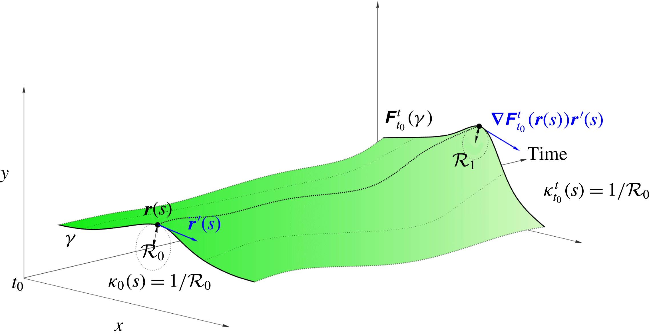
(see figure 4 for illustration).
Curvature evolution along a material line
 $\unicode[STIX]{x1D6FE}$
in the extended phase space of position and time.

The normalized tangent vector to the advected curve
 $\unicode[STIX]{x1D641}_{t_{0}}^{t}(\unicode[STIX]{x1D6FE})$
, as a function of
 $\boldsymbol{r}(s)$
, can be computed as
 $$\begin{eqnarray}\tilde{\boldsymbol{r}}^{\prime }(s)=\frac{\unicode[STIX]{x1D735}\unicode[STIX]{x1D641}_{t_{0}}^{t}(\boldsymbol{r}(s))\boldsymbol{r}^{\prime }(s)}{|\unicode[STIX]{x1D735}\unicode[STIX]{x1D641}_{t_{0}}^{t}(\boldsymbol{r}(s))\boldsymbol{r}^{\prime }(s)|}=\frac{\unicode[STIX]{x1D735}\unicode[STIX]{x1D641}_{t_{0}}^{t}(\boldsymbol{r}(s))\boldsymbol{r}^{\prime }(s)}{\sqrt{\langle \boldsymbol{r}^{\prime }(s),\unicode[STIX]{x1D63E}_{t_{0}}^{t}(\boldsymbol{r}(s))\boldsymbol{r}^{\prime }(s)\rangle }},\end{eqnarray}$$
and the arclength of
 $\unicode[STIX]{x1D641}_{t_{0}}^{t}(\unicode[STIX]{x1D6FE})$
from
 $\unicode[STIX]{x1D641}_{t_{0}}^{t}(\boldsymbol{r}(s_{1}))$
to
 $\unicode[STIX]{x1D641}_{t_{0}}^{t}(\boldsymbol{r}(s))$
is
 $$\begin{eqnarray}\tilde{s}=\int _{s_{1}}^{s}\sqrt{\langle \boldsymbol{r}^{\prime }(\unicode[STIX]{x1D70F}),\unicode[STIX]{x1D63E}_{t_{0}}^{t}(\boldsymbol{r}(\unicode[STIX]{x1D70F}))\boldsymbol{r}^{\prime }(\unicode[STIX]{x1D70F})\rangle }\,\text{d}\unicode[STIX]{x1D70F},\end{eqnarray}$$
where
 $\langle \cdot \,,\cdot \rangle$
denotes the Euclidean inner product. Using (3.1)–(3.2), we obtain the curvature vector of
 $\unicode[STIX]{x1D641}_{t_{0}}^{t}(\unicode[STIX]{x1D6FE})$
in the form
 $$\begin{eqnarray}\tilde{\unicode[STIX]{x1D73F}}(s)=\frac{\text{d}}{\text{d}\tilde{s}}\tilde{\boldsymbol{r}}^{\prime }=\frac{\text{d}s}{\text{d}\tilde{s}}\frac{\text{d}}{\text{d}s}\tilde{\boldsymbol{r}}^{\prime }=\frac{\tilde{\boldsymbol{r}}^{\prime \prime }(s)}{\sqrt{\langle \boldsymbol{r}^{\prime }(s),\unicode[STIX]{x1D63E}_{t_{0}}^{t}(\boldsymbol{r}(s))\boldsymbol{r}^{\prime }(s)\rangle }}.\end{eqnarray}$$
Finally, projecting
 $\tilde{\unicode[STIX]{x1D73F}}(s)$
onto the curve-normal direction, we obtain the material evolution of the curvature scalar
 $\unicode[STIX]{x1D705}_{t_{0}}^{t}(s)$
along
 $\unicode[STIX]{x1D6FE}$
, as a function of its parametrization at the initial time, in the form
 $$\begin{eqnarray}\unicode[STIX]{x1D705}_{t_{0}}^{t}(s)=\langle \tilde{\unicode[STIX]{x1D73F}}(s),\unicode[STIX]{x1D64D}\tilde{\boldsymbol{r}}^{\prime }(s)\rangle .\end{eqnarray}$$
Similarly, the material curvature rate
 $\dot{\unicode[STIX]{x1D705}}_{t_{0}}(s)$
along
 $\unicode[STIX]{x1D6FE}$
advected under the flow
 $\unicode[STIX]{x1D641}_{t_{0}}^{t}(\unicode[STIX]{x1D6FE})$
, at the initial time
 $t_{0}$
, can be computed as
 $$\begin{eqnarray}\dot{\unicode[STIX]{x1D705}}_{t_{0}}(s)=\frac{\text{d}}{\text{d}t}\unicode[STIX]{x1D705}_{t_{0}}^{t}(s)|_{t=t_{0}}.\end{eqnarray}$$
Figure 4 illustrates formula (3.4). Using the formulae derived in appendix A together with the results of this section, we obtain the following result.
Theorem 1. Consider a smooth material curve
 $\unicode[STIX]{x1D6FE}\subset U$
parametrized at
 $t_{0}$
in the form
 $\boldsymbol{r}(s)$
,
 $s\in [s_{1},s_{2}]\subset \mathbb{R}$
, and denote its local tangent vector by
 $\boldsymbol{r}^{\prime }(s)$
and curvature scalar by
 $\unicode[STIX]{x1D705}_{0}(s):=\unicode[STIX]{x1D705}_{t_{0}}^{t_{0}}(s)=\langle \boldsymbol{r}^{\prime \prime }(s),\unicode[STIX]{x1D64D}\boldsymbol{r}^{\prime }(s)\rangle /\sqrt{\langle \boldsymbol{r}^{\prime }(s),\boldsymbol{ r}^{\prime }(s)\rangle }^{3}$
. The curvature evolution along
 $\unicode[STIX]{x1D6FE}$
, under the action of the flow map
 $\unicode[STIX]{x1D641}_{t_{0}}^{t}$
, can then be computed as
 $$\begin{eqnarray}\unicode[STIX]{x1D705}_{t_{0}}^{t}=\frac{\langle (\unicode[STIX]{x1D735}^{2}\unicode[STIX]{x1D641}_{t_{0}}^{t}(\boldsymbol{r})\boldsymbol{r}^{\prime })\boldsymbol{r}^{\prime },\unicode[STIX]{x1D64D}\unicode[STIX]{x1D735}\unicode[STIX]{x1D641}_{t_{0}}^{t}(\boldsymbol{r})\boldsymbol{r}^{\prime }\rangle }{\langle \boldsymbol{r}^{\prime },\unicode[STIX]{x1D63E}_{t_{0}}^{t}(\boldsymbol{r})\boldsymbol{r}^{\prime }\rangle ^{3/2}}+\unicode[STIX]{x1D705}_{0}\det [\unicode[STIX]{x1D735}\unicode[STIX]{x1D641}_{t_{0}}^{t}(\boldsymbol{r})]\frac{\langle \boldsymbol{r}^{\prime },\boldsymbol{r}^{\prime }\rangle ^{3/2}}{\langle \boldsymbol{r}^{\prime },\unicode[STIX]{x1D63E}_{t_{0}}^{t}(\boldsymbol{r})\boldsymbol{r}^{\prime }\rangle ^{3/2}}\end{eqnarray}$$
and the material curvature rate as
 $$\begin{eqnarray}\dot{\unicode[STIX]{x1D705}}_{t_{0}}=\underbrace{\frac{\langle \unicode[STIX]{x1D64D}\boldsymbol{r}^{\prime },(\unicode[STIX]{x1D735}\unicode[STIX]{x1D64E}(\boldsymbol{r},t_{0})\boldsymbol{r}^{\prime })\boldsymbol{r}^{\prime }\rangle }{\langle \boldsymbol{r}^{\prime },\boldsymbol{r}^{\prime }\rangle ^{3/2}}}_{\dot{\unicode[STIX]{x1D705}}_{I}}-\underbrace{\frac{\langle \unicode[STIX]{x1D735}\unicode[STIX]{x1D714}(\boldsymbol{r},t_{0}),\boldsymbol{r}^{\prime }\rangle }{2\langle \boldsymbol{r}^{\prime },\boldsymbol{r}^{\prime }\rangle ^{1/2}}}_{\dot{\unicode[STIX]{x1D705}}_{II}}+\underbrace{\unicode[STIX]{x1D705}_{0}\left[\unicode[STIX]{x1D735}\boldsymbol{\cdot }\boldsymbol{f}(\boldsymbol{r},t_{0})-3\frac{\langle \boldsymbol{r}^{\prime },\unicode[STIX]{x1D64E}(\boldsymbol{r},t_{0})\boldsymbol{r}^{\prime }\rangle }{\langle \boldsymbol{r}^{\prime },\boldsymbol{r}^{\prime }\rangle }\right]}_{\dot{\unicode[STIX]{x1D705}}_{III}},\end{eqnarray}$$
where
 $(\unicode[STIX]{x1D735}\unicode[STIX]{x1D64E}(\boldsymbol{r},t_{0})\boldsymbol{r}^{\prime })_{ij}=\sum _{k=1}^{2}\unicode[STIX]{x1D61A}_{ij,k}(\boldsymbol{r},t_{0})\boldsymbol{r}_{k}^{\prime },i,j\in \{1,2\}$
. For incompressible flows (i.e.
 $\unicode[STIX]{x1D735}\boldsymbol{\cdot }\boldsymbol{f}=0$
) and under arclength parametrization of
 $\unicode[STIX]{x1D6FE}$
(i.e.
 $\langle \boldsymbol{r}^{\prime },\boldsymbol{r}^{\prime }\rangle =1$
), (3.6) and (3.7) simplify to
 $$\begin{eqnarray}\displaystyle & \displaystyle \unicode[STIX]{x1D705}_{t_{0}}^{t}=\frac{\langle (\unicode[STIX]{x1D735}^{2}\unicode[STIX]{x1D641}_{t_{0}}^{t}(\boldsymbol{r})\boldsymbol{r}^{\prime })\boldsymbol{r}^{\prime },\unicode[STIX]{x1D64D}\unicode[STIX]{x1D735}\unicode[STIX]{x1D641}_{t_{0}}^{t}(\boldsymbol{r})\boldsymbol{r}^{\prime }\rangle }{\langle \boldsymbol{r}^{\prime },\unicode[STIX]{x1D63E}_{t_{0}}^{t}(\boldsymbol{r})\boldsymbol{r}^{\prime }\rangle ^{3/2}}+\frac{\unicode[STIX]{x1D705}_{0}}{\langle \boldsymbol{r}^{\prime },\unicode[STIX]{x1D63E}_{t_{0}}^{t}(\boldsymbol{r})\boldsymbol{r}^{\prime }\rangle ^{3/2}}, & \displaystyle\end{eqnarray}$$
 $$\begin{eqnarray}\displaystyle & \displaystyle \dot{\unicode[STIX]{x1D705}}_{t_{0}}=\langle (\unicode[STIX]{x1D735}\unicode[STIX]{x1D64E}(\boldsymbol{r},t_{0})\boldsymbol{r}^{\prime })\boldsymbol{r}^{\prime },\unicode[STIX]{x1D64D}\boldsymbol{r}^{\prime }\rangle -{\textstyle \frac{1}{2}}\langle \unicode[STIX]{x1D735}\unicode[STIX]{x1D714}(\boldsymbol{r},t_{0}),\boldsymbol{r}^{\prime }\rangle -3\unicode[STIX]{x1D705}_{0}\langle \boldsymbol{r}^{\prime },\unicode[STIX]{x1D64E}(\boldsymbol{r},t_{0})\boldsymbol{r}^{\prime }\rangle . & \displaystyle\end{eqnarray}$$
Proof. See appendix A.◻
Equation (3.7) shows that the curvature rate
 $\dot{\unicode[STIX]{x1D705}}_{t_{0}}(s)$
along
 $\unicode[STIX]{x1D6FE}$
consists of three terms: the topology of the stretching rate (
 $\dot{\unicode[STIX]{x1D705}}_{I}$
), the topology of the rigid-body rotation rate described by the vorticity (
 $\dot{\unicode[STIX]{x1D705}}_{II}$
) and the compressibility of
 $\boldsymbol{f}$
together with the stretching rate along
 $\unicode[STIX]{x1D6FE}$
, weighted by its current curvature (
 $\dot{\unicode[STIX]{x1D705}}_{III}$
). Therefore, the curvature rate
 $\dot{\unicode[STIX]{x1D705}}$
, and hence also the curvature map
 $\unicode[STIX]{x1D705}_{t_{0}}^{t}$
, combines stretching- and rotation-based quantities.
The computation of spatial derivatives of
 $\unicode[STIX]{x1D641}_{t_{0}}^{t}$
in (3.6) is a numerically sensitive procedure. To this end, in appendix B, we derive general identities that allow us to compute
 $\unicode[STIX]{x1D705}_{t_{0}}^{t}$
without taking spatial derivatives of
 $\unicode[STIX]{x1D641}_{t_{0}}^{t}$
numerically. In appendix C, we show that
 $\dot{\unicode[STIX]{x1D705}}$
and
 $\unicode[STIX]{x1D705}_{t_{0}}^{t}$
are independent of the parametrization of
 $\unicode[STIX]{x1D6FE}$
and are objective, i.e. remain unchanged under time-dependent rotations and translations of the coordinate frame. This follows from the objectivity of the rate-of-strain tensor and the objectivity of the vorticity gradient. Remarkably, although vorticity is not objective, its topology described by the vorticity gradient is objective. We summarize these results as follows.
Proposition 1. The material curvature rate
 $\dot{\unicode[STIX]{x1D705}}_{t_{0}}$
and the curvature map
 $\unicode[STIX]{x1D705}_{t_{0}}^{t}$
(i) are independent of the parametrization
 $\boldsymbol{r}(s)$
,
$s\in [s_{1},s_{2}]\subset \mathbb{R}$
;
(ii) are objective, i.e. invariant under coordinate changes of the form
(3.10)where$$\begin{eqnarray}\boldsymbol{z}=\unicode[STIX]{x1D64C}(t)\tilde{\boldsymbol{z}}+\boldsymbol{b}(t),\end{eqnarray}$$
$\unicode[STIX]{x1D64C}(t)\in SO(2)$
and
$\boldsymbol{b}(t)\in \mathbb{R}^{2}$
are smooth functions of time.


Proof. See appendix C.◻
Proposition 1 guarantees that flow features inferred from
 $\dot{\unicode[STIX]{x1D705}}$
and
 $\unicode[STIX]{x1D705}_{t_{0}}^{t}$
are tied to evolving fluid particles without any reference to coordinates or parametrization. This frame-invariance property is a basic axiom of continuum mechanics (Gurtin Reference Gurtin1982), ensuring that the material response of a deforming continuum, including the formation of a material spike driving flow separation, is independent of the observer.
4 The backbone of flow separation
As illustrated in figures 1 and 3, the birth of flow separation occurs at a location different from the separation point identified by earlier asymptotic theories, even in steady flows. Here, we seek to describe how an initial upwelling along the boundary turns into a material spike that later converges to a long-term separation profile predicted by Prandtl’s theory for steady flows (Prandtl Reference Prandtl1904) and by the kinematic theory of separation for unsteady flows (Haller Reference Haller2004).
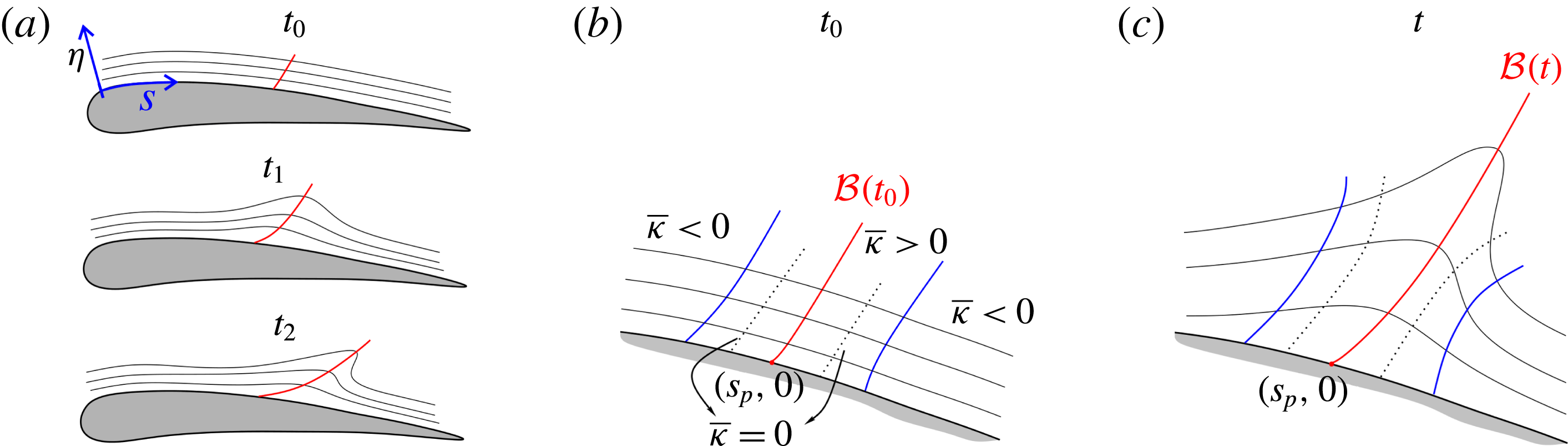
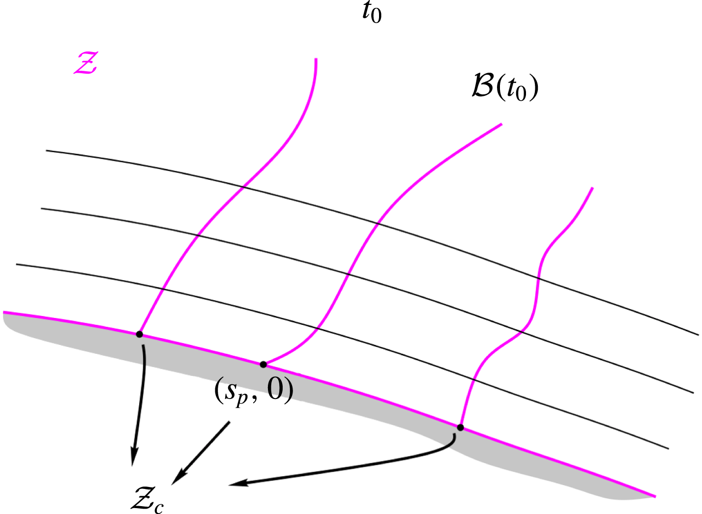
(a) Sketch of the typical shape of initially boundary-parallel material lines (black) in the proximity of a wing profile before and after flow separation. Red lines show the backbone
 ${\mathcal{B}}(t)$
of the evolving material spike. (b) Sketch of the typical topology of the curvature change map defined by (4.2) in a neighbourhood of the backbone of separation
 ${\mathcal{B}}(t_{0})$
at the initial time. (c) Advected time-
 $t$
position of the features in (b) for
 $t\in [t_{0},t_{0}+T]$
.

The observed backbone of separation is characterized by points of maximal curvature change (relative to the initial curvature) along boundary-parallel material lines in a neighbourhood of the no-slip boundary over the time interval
 $[t_{0},t]$
(cf. figure 5
a). To express this coherence principle mathematically, we consider a curved wall and a curvilinear coordinate system
 $(s,\unicode[STIX]{x1D702})$
, in which the wall is defined as
 $$\begin{eqnarray}{\mathcal{W}}:=\{(s,\unicode[STIX]{x1D702})\in [s_{1},s_{2}]\times [0,\unicode[STIX]{x1D702}_{1}]:\unicode[STIX]{x1D702}=0\}.\end{eqnarray}$$
Next, we consider a foliation of a neighbourhood of the boundary by material curves parallel to the wall at the initial time, parametrized in the form
 $\boldsymbol{r}_{\unicode[STIX]{x1D702}}(s)$
, where
 $s\in [s_{1},s_{2}]\subset \mathbb{R}$
,
 $\unicode[STIX]{x1D702}\in [0,\unicode[STIX]{x1D702}_{1}]$
,
 $\unicode[STIX]{x1D702}_{1}>0$
. We denote the tangent vectors and curvature scalars of these curves by
 $\boldsymbol{r}_{\unicode[STIX]{x1D702}}^{\prime }(s)$
and
 $\unicode[STIX]{x1D705}_{0_{\unicode[STIX]{x1D702}}}(s)$
. With our definition of
 $\unicode[STIX]{x1D64D}$
in (2.3), together with the clockwise parametrization of the boundary (cf. figure 5
a), the curvature scalar defined by (3.4) is taken with respect to normal vectors pointing towards the boundary.
Substituting
 $\boldsymbol{r}_{\unicode[STIX]{x1D702}}^{\prime }$
and
 $\unicode[STIX]{x1D705}_{0_{\unicode[STIX]{x1D702}}}$
into (3.6) and subtracting the initial curvature, we obtain the curvature change
 $\overline{\unicode[STIX]{x1D705}}_{t_{0}}^{t}(s,\unicode[STIX]{x1D702})$
of the foliation over
 $[t_{0},t]$
,
 $$\begin{eqnarray}\overline{\unicode[STIX]{x1D705}}_{t_{0}}^{t}:=\unicode[STIX]{x1D705}_{t_{0}}^{t}-\unicode[STIX]{x1D705}_{0}=\frac{\langle (\unicode[STIX]{x1D735}^{2}\unicode[STIX]{x1D641}_{t_{0}}^{t}(\boldsymbol{r}_{\unicode[STIX]{x1D702}})\boldsymbol{r}_{\unicode[STIX]{x1D702}}^{\prime })\boldsymbol{r}_{\unicode[STIX]{x1D702}}^{\prime },\unicode[STIX]{x1D64D}\unicode[STIX]{x1D735}\unicode[STIX]{x1D641}_{t_{0}}^{t}(\boldsymbol{r}_{\unicode[STIX]{x1D702}})\boldsymbol{r}_{\unicode[STIX]{x1D702}}^{\prime }\rangle }{\langle \boldsymbol{r}_{\unicode[STIX]{x1D702}}^{\prime },\unicode[STIX]{x1D63E}_{t_{0}}^{t}(\boldsymbol{r}_{\unicode[STIX]{x1D702}})\boldsymbol{r}_{\unicode[STIX]{x1D702}}^{\prime }\rangle ^{3/2}}+\unicode[STIX]{x1D705}_{0_{\unicode[STIX]{x1D702}}}\left[\frac{\det (\unicode[STIX]{x1D735}\unicode[STIX]{x1D641}_{t_{0}}^{t}(\boldsymbol{r}_{\unicode[STIX]{x1D702}}))\langle \boldsymbol{r}_{\unicode[STIX]{x1D702}}^{\prime },\boldsymbol{r}_{\unicode[STIX]{x1D702}}^{\prime }\rangle ^{3/2}}{\langle \boldsymbol{r}_{\unicode[STIX]{x1D702}}^{\prime },\unicode[STIX]{x1D63E}_{t_{0}}^{t}(\boldsymbol{r}_{\unicode[STIX]{x1D702}})\boldsymbol{r}_{\unicode[STIX]{x1D702}}^{\prime }\rangle ^{3/2}}-1\right].\end{eqnarray}$$
From this definition of
 $\overline{\unicode[STIX]{x1D705}}_{t_{0}}^{t}$
, it follows that
 $$\begin{eqnarray}\frac{\text{d}}{\text{d}t}\overline{\unicode[STIX]{x1D705}}_{t_{0}}^{t}(s,\unicode[STIX]{x1D702})|_{t=t_{0}}=\dot{\unicode[STIX]{x1D705}}_{t_{0}}(s,\unicode[STIX]{x1D702}).\end{eqnarray}$$
Thus, the time derivative of the Lagrangian curvature change coincides with the curvature rate defined by (3.7). Because of the no-slip condition, the wall is an invariant set of (2.1), which implies
 $$\begin{eqnarray}\left.\begin{array}{@{}c@{}}\displaystyle \overline{\unicode[STIX]{x1D705}}_{t_{0}}^{t}(s,0)\equiv 0,\quad \unicode[STIX]{x2202}_{s^{i}}\overline{\unicode[STIX]{x1D705}}_{t_{0}}^{t}(s,0),\\ \displaystyle \dot{\unicode[STIX]{x1D705}}_{t_{0}}(s,0)\equiv 0,\quad \unicode[STIX]{x2202}_{s^{i}}\dot{\unicode[STIX]{x1D705}}_{t_{0}}(s,0),\quad \unicode[STIX]{x2202}_{s^{i}}:=\frac{\unicode[STIX]{x2202}^{i}}{\unicode[STIX]{x2202}s^{i}}\end{array}\right\}\end{eqnarray}$$
along the wall, for any positive integer
 $i$
.
4.1 The Lagrangian backbone of the separation spike
We now use the curvature change
 $\overline{\unicode[STIX]{x1D705}}_{t_{0}}^{t}$
to define the Lagrangian backbone of a material spike as its theoretical centrepiece over a fixed time interval
 $[t_{0},t_{0}+T]$
, as illustrated in figure 5(a). The following definition introduces a formal mathematical characterization of such a centrepiece.
Definition 1. The Lagrangian backbone
 ${\mathcal{B}}(t)$
of separation is the theoretical centrepiece of the material spike over the time interval
 $[t_{0},t_{0}+T]$
. The backbone
 ${\mathcal{B}}(t)$
is an evolving material line whose initial position
 ${\mathcal{B}}(t_{0})$
is a positive-valued wall-transverse ridge of the
 $\overline{\unicode[STIX]{x1D705}}_{t_{0}}^{t_{0}+T}$
field.
In this context, a ridge is a set of points that are positive local maxima of
 $\overline{\unicode[STIX]{x1D705}}_{t_{0}}^{t_{0}+T}$
along
 $\unicode[STIX]{x1D702}=\text{const}$
. curves, and can be computed as described in Proposition 2.
Figure 5(b) illustrates the topology of
 $\overline{\unicode[STIX]{x1D705}}_{t_{0}}^{t_{0}+T}(s,\unicode[STIX]{x1D702})$
in a neighbourhood of the wall, with the loci of maximal curvature change along each
 $\unicode[STIX]{x1D702}=\text{const}$
. line forming the curve
 ${\mathcal{B}}(t_{0})$
. The backbone is typically located between two curves of minimal negative curvature change, shown in blue. By continuity of
 $\overline{\unicode[STIX]{x1D705}}_{t_{0}}^{t_{0}+T}$
, there also exists a zero curve of
 $\overline{\unicode[STIX]{x1D705}}_{t_{0}}^{t_{0}+T}$
in the vicinity of
 ${\mathcal{B}}(t_{0})$
, as shown in dashed black. Figure 5(c) shows the advected images of the material curves shown in figure 5(b), under the action of the flow map
 $\unicode[STIX]{x1D641}_{t_{0}}^{t}$
. The material spike geometry sketched in figure 5 is consistent with the ones observed numerically in figures 1 and 2.
Of particular interest to us is the Lagrangian spiking point
 $$\begin{eqnarray}(s_{p},0):={\mathcal{B}}(t_{0})\cap {\mathcal{W}},\end{eqnarray}$$
the point where the backbone of separation connects to the wall (cf. figure 5). Because
 $\overline{\unicode[STIX]{x1D705}}_{t_{0}}^{t_{0}+T}(s,0)\equiv 0$
at the wall,
 $(s_{p},0)$
is a distinguished point on the wall with positive maximal curvature change in the limit of
 $\unicode[STIX]{x1D702}\rightarrow 0$
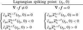
. In appendix D, we derive explicit formulae for the spiking point on a flat no-slip boundary in the case of compressible and incompressible flows. We summarize our results in tables 2–4. Specifically, table 2 describes the location of
 $(s_{p},0)$
in terms of the curvature change function.
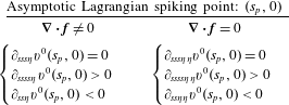
Equations determining the Lagrangian spiking point on a flat no-slip boundary in terms of the Lagrangian curvature change
 $\overline{\unicode[STIX]{x1D705}}_{t_{0}}^{t_{0}+T}$
for compressible and incompressible flows over the time interval
 $[t_{0},t_{0}+T]$
.
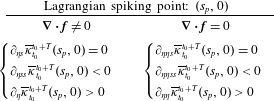
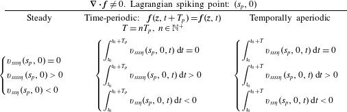
In tables 3 and 4, we give an equivalent formulation of the results in table 2 in terms of averaged Eulerian quantities in the case of steady, time-periodic and unsteady flows. We have briefly introduced the results of table 4 already in § 1.2.
The same as the left column of table 2, but expressed in terms of averaged Eulerian quantities.

The same as the right column of table 2, but expressed in terms of averaged Eulerian quantities.

In our definition of
 $(s_{p},0)$
, the first two conditions ensure that
 $(s_{p},0)$
is a maximum of the curvature change
 $\overline{\unicode[STIX]{x1D705}}_{t_{0}}^{t_{0}+T}$
, and the third one ensures that the curvature change at
 $(s_{p},0)$
is positive, i.e. wall-parallel material lines undergo upwelling-type deformation.
The formulae in tables 3 and 4 highlight three important facts. First, in the case of steady flows, the spiking pointy is fixed, independent of
 $T$
, and can be computed from derivatives of the velocity field on the wall. Second, in the case of
 $T_{p}$
-periodic flows, with
 $T$
equal to any arbitrary multiple of
 $T_{p}$
, the spiking point is fixed, independent of
 $t_{0}$
, and can be computed by averaging derivatives of the velocity field on the wall over one period. Third, for general unsteady flows or time-periodic flows with
 $T\neq nT_{p},n\in \mathbb{N}^{+}$
, the spiking point moves depending on
 $t_{0}$
and
 $T$
, and can be computed by averaging derivatives of the velocity field over
 $[t_{0},t_{0}+T]$
. We summarize the results of this section in the following proposition.
Proposition 2. Over the finite time interval
 $[t_{0},t_{0}+T]$
, we have the following.
(i) The initial position
${\mathcal{B}}(t_{0})$
of the Lagrangian backbone of separation can be computed as the set of points
$s\in [s_{1},s_{2}]$
,
$\unicode[STIX]{x1D702}\in [0,\unicode[STIX]{x1D702}_{1}]$
, (4.6)The Lagrangian spiking point$$\begin{eqnarray}{\mathcal{B}}(t_{0}):=\left\{\begin{array}{@{}ll@{}}\unicode[STIX]{x2202}_{s}\overline{\unicode[STIX]{x1D705}}_{t_{0}}^{t_{0}+T}(s,\unicode[STIX]{x1D702})=0,\quad & \unicode[STIX]{x1D702}\in (0,\unicode[STIX]{x1D702}_{1}],\\ \unicode[STIX]{x2202}_{ss}\overline{\unicode[STIX]{x1D705}}_{t_{0}}^{t_{0}+T}(s,\unicode[STIX]{x1D702})<0,\quad & \unicode[STIX]{x1D702}\in (0,\unicode[STIX]{x1D702}_{1}],\\ \overline{\unicode[STIX]{x1D705}}_{t_{0}}^{t_{0}+T}(s,\unicode[STIX]{x1D702})>0,\quad & \unicode[STIX]{x1D702}\in (0,\unicode[STIX]{x1D702}_{1}],\\ (s_{p},\unicode[STIX]{x1D702}),\quad & \unicode[STIX]{x1D702}=0.\end{array}\right.\end{eqnarray}$$
$(s_{p},0)$
can be computed in terms of Lagrangian quantities using the formulae in table 2, in terms of averaged Eulerian quantities using the formulae in tables 3 and 4, or as the intersection of
${\mathcal{B}}(t_{0})$
with the no-slip boundary (cf. (4.5)).(ii) Later positions
${\mathcal{B}}(t)$
of the Lagrangian backbone of separation can be computed as
${\mathcal{B}}(t)=\unicode[STIX]{x1D641}_{t_{0}}^{t}({\mathcal{B}}(t_{0}))$
,
$t\in [t_{0},t_{0}+T]$
.(iii) The Lagrangian spiking point
$(s_{p},0)$





By Proposition 1, the Lagrangian backbone of separation is objective. Although the analytic formulae in tables 3 and 4 involve higher derivatives of the velocity field, the spiking point can also be identified as the intersection of
 ${\mathcal{B}}(t_{0})$
with the wall (cf. (4.5)) with low numerical effort.
While our main interest is to capture the birth of material spikes, in appendix D.3, we also derive explicit formulae for the asymptotic
 $(T\rightarrow \infty )$
mean location of the Lagrangian spiking point in the case of general unsteady velocity fields that admit a finite asymptotic mean, such as periodic and quasiperiodic velocity fields. The latter is relevant for several separation problems, such as separation behind a cylinder or a backward facing step, which admit a finite number of dominant frequencies in their Fourier spectra. In these flows, we find that the asymptotic Lagrangian spiking point oscillates with respect to a well-defined mean position. We summarize these formulae in table 6. In the case of steady and time-periodic velocity fields, we recover the formulae in tables 3 and 4 because the Lagrangian spiking point is fixed, as noted in Proposition 2.
For incompressible flows, we derive in appendix F an approximate velocity field
 $\overline{\boldsymbol{f}}(\boldsymbol{z},t)$
near the boundary. With the help of this approximate velocity field, we express
 $\overline{\boldsymbol{f}}(\boldsymbol{z},t)$
in terms of the wall pressure, the skin friction, and their temporal and spatial derivatives along the wall. Therefore, replacing
 $\boldsymbol{f}(\boldsymbol{z},t)$
(cf. (2.1)) with
 $\overline{\boldsymbol{f}}(\boldsymbol{z},t)$
(cf. (F 8)) allows us to compute the backbone of separation in the proximity of the boundary from wall-based quantities. For more advanced velocity estimation techniques, such as adjoint-based methods and reduced-rank extended Kalman filters, see, e.g., Bewley & Protas (Reference Bewley and Protas2004).
4.2 The Eulerian backbone of the separation spike
Over an infinitesimally short time interval, we now introduce the instantaneous notion of the backbone of separation. This Eulerian concept follows by taking the time derivative of the Lagrangian backbone of separation and evaluating it at
 $T=0$
.
Definition 2. At a time instant
 $t\in [t_{0},t_{0}+T]$
, the Eulerian backbone of separation
 ${\mathcal{B}}_{E}(t)$
is the theoretical centrepiece of the material spike over an infinitesimally short time interval. The Eulerian backbone of separation is a positive-valued wall-transverse maximum ridge of the
 $\dot{\unicode[STIX]{x1D705}}_{t}$
field.
In other words,
 ${\mathcal{B}}_{E}(t)$
consists of the set of points where the instantaneous curvature rate is positive and attains a local maximum along each
 $\unicode[STIX]{x1D702}=\text{const}$
. curve, and can be computed as described in Proposition 3.
Similarly to the Lagrangian case, we define the Eulerian spiking point at time
 $t$
as
 $$\begin{eqnarray}(s_{pE},0):={\mathcal{B}}_{E}(t)\cap {\mathcal{W}},\end{eqnarray}$$
i.e. the point where the Eulerian backbone of separation connects to the wall. Because
 $\dot{\unicode[STIX]{x1D705}}_{t}(s,0)\equiv 0$
,
 $(s_{pE},0)$
is a distinguished point on the wall with positive maximal curvature rate in the limit of
 $\unicode[STIX]{x1D702}\rightarrow 0$
. For a flat wall, we derive analytic expressions for
 $(s_{pE},0)$
in appendix E, which are summarized in table 5.
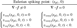
Exact criteria for the Eulerian spiking point on a flat no-slip boundary at a time instant
 $t$
, for compressible and incompressible flows.

For steady flows, comparing the formula of
 $(s_{pE},0)$
(cf. table 5) with the one of
 $(s_{p},0)$
(cf. tables 3 and 4), we obtain that the Lagrangian and Eulerian backbones of separation connect to the wall at the same location, i.e.
 $s_{pE}\equiv s_{p}$
(see, e.g., figure 7). We summarize the results of this section in the following proposition.
Proposition 3. At a time instant
 $t\in [t_{0},t_{0}+T]$
, we have the following.
(i) The Eulerian backbone of separation
${\mathcal{B}}_{E}(t)$
can be computed as the set of points
$s\in [s_{1},s_{2}]$
,
$\unicode[STIX]{x1D702}\in [0,\unicode[STIX]{x1D702}_{1}]$
, (4.8)The Eulerian spiking point$$\begin{eqnarray}{\mathcal{B}}_{E}(t):=\left\{\begin{array}{@{}ll@{}}\unicode[STIX]{x2202}_{s}\dot{\unicode[STIX]{x1D705}}_{t}(s,\unicode[STIX]{x1D702})=0,\quad & \unicode[STIX]{x1D702}\in (0,\unicode[STIX]{x1D702}_{1}],\\ \unicode[STIX]{x2202}_{ss}\dot{\unicode[STIX]{x1D705}}_{t}(s,\unicode[STIX]{x1D702})<0,\quad & \unicode[STIX]{x1D702}\in (0,\unicode[STIX]{x1D702}_{1}],\\ \dot{\unicode[STIX]{x1D705}}_{t}(s,\unicode[STIX]{x1D702})>0,\quad & \unicode[STIX]{x1D702}\in (0,\unicode[STIX]{x1D702}_{1}],\\ (s_{pE},\unicode[STIX]{x1D702}),\quad & \unicode[STIX]{x1D702}=0.\end{array}\right.\end{eqnarray}$$
$(s_{pE},0)$
can be computed from the formulae in table 5, or as the intersection of
${\mathcal{B}}_{E}(t)$
with the no-slip boundary (cf. (4.7)).(ii) The Eulerian spiking point coincides with the Lagrangian spiking point in steady flows.


By Proposition 1, the Eulerian backbone of separation is objective. Following the same argument as § 4.1, although the analytic formulae in table 5 involve higher derivatives of the velocity field, the spiking point can also be identified with low numerical effort directly from (4.7), as the intersection of
 ${\mathcal{B}}_{E}(t)$
with the wall.
5 Numerical schemes
Here we summarize the numerical steps in locating the Lagrangian and Eulerian backbones of separation in a general two-dimensional compressible flow. For a MATLAB implementation of our method, we also indicate the relevant built-in functions that we use.


Our kinematic theory depends neither on governing equations generating the velocity field nor on the particular flow regime. At high Reynolds numbers, however, filtering out the high frequencies in the velocity field may be necessary for identifying the ridges marking multiple material spikes.
6 Examples
We now use Algorithms 1 and 2 from § 5 to locate the Lagrangian and Eulerian backbones of separation in two-dimensional analytical and experimental velocity fields with flat and curved no-slip boundaries.
6.1 Separation induced by a rotating and translating cylinder
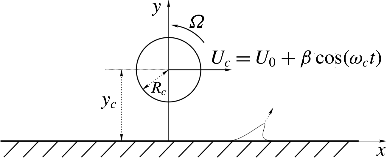
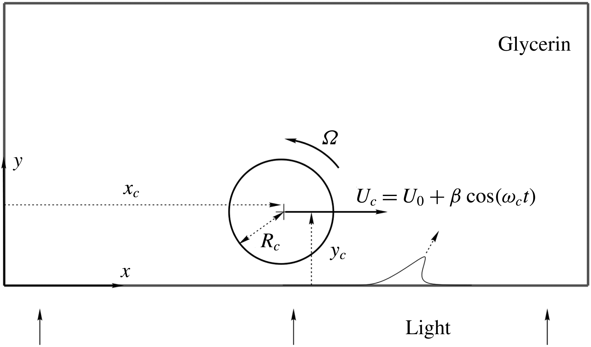
We consider the creeping flow developing around a rotating and translating circular cylinder moving close to a plane wall (Klonowska-Prosnak & Prosnak Reference Klonowska-Prosnak and Prosnak2001; Miron & Vétel Reference Miron and Vétel2015). We summarize the details of this flow in appendix G and sketch the flow set-up in figure 6. A cylinder of radius
 $R_{c}$
, whose centre is initially at position
 $(0,y_{c})$
, rotates about its axis at a constant angular velocity
 $\unicode[STIX]{x1D6FA}$
, and translates in the
 $x$
direction with velocity
 ${\dot{x}}_{c}=U_{c}=U_{0}+\unicode[STIX]{x1D6FD}\cos (\unicode[STIX]{x1D714}_{c}t)$
. Depending on the parameters
 $\unicode[STIX]{x1D6FA},U_{0},\unicode[STIX]{x1D6FD}$
and
 $\unicode[STIX]{x1D714}_{c}$
, this simple set-up allows us to generate steady, time-periodic and unsteady flows, and hence to simulate fixed and moving separation on the wall downstream of the cylinder. Throughout this section, we use
 $R_{c}=1$
and
 $y_{c}=2$
.
6.1.1 Steady flow
We first let
 $\unicode[STIX]{x1D6FA}=20$
and
 $U_{0}=\unicode[STIX]{x1D6FD}=0$
, and therefore assume that the cylinder rotates without translation
 $(U_{c}=0)$
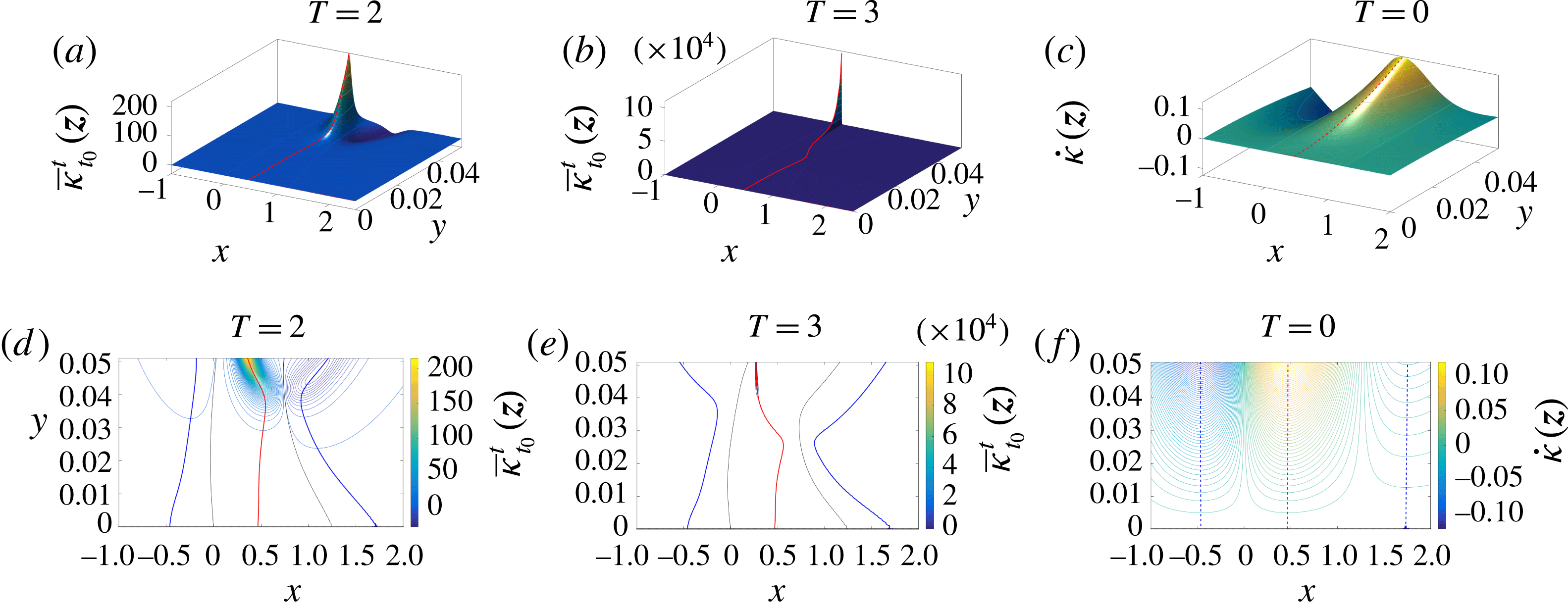
, generating a steady flow. Figure 1 shows the streamlines of this flow. Figure 7 shows the initial positions of the Lagrangian backbone of separation for two different integration times, as well as the Eulerian backbones of separation. Specifically, (a–c) show the Lagrangian curvature change fields
 $\overline{\unicode[STIX]{x1D705}}_{t_{0}}^{t_{0}+T}(\boldsymbol{z})$
for
 $T=2$
and
 $T=3$
, and the curvature rate field
 $\dot{\unicode[STIX]{x1D705}}(\boldsymbol{z})$
that corresponds to the time derivative of
 $\overline{\unicode[STIX]{x1D705}}_{t_{0}}^{t_{0}+T}(\boldsymbol{z})$
, evaluated at
 $T=0$
. Panels (d–f) show the contour plots of the corresponding scalar fields. The initial position
 ${\mathcal{B}}(0)$
of the Lagrangian backbone of separation, i.e. the positive ridge of
 $\overline{\unicode[STIX]{x1D705}}_{t_{0}}^{t_{0}+T}(\boldsymbol{z})$
, is shown in red, the loci of minimal signed curvature in the vicinity of
 ${\mathcal{B}}(0)$
are shown in blue and the zero set of
 $\overline{\unicode[STIX]{x1D705}}_{t_{0}}^{t_{0}+T}(\boldsymbol{z})$
is shown in black, as sketched in figure 5(b). Similarly, the Eulerian backbone of separation
 ${\mathcal{B}}_{E}(0)$
is shown in dashed red and the locus of minimal signed curvature rate in dashed blue.
Separation induced by a rotating and translating cylinder: flow set-up and parameters.

(a) Lagrangian curvature change field
 $\overline{\unicode[STIX]{x1D705}}_{t_{0}}^{t_{0}+T}(\boldsymbol{z})$
for
 $T=2$
. (b) The same as (a) for
 $T=3$
. (c) Time derivative of
 $\overline{\unicode[STIX]{x1D705}}_{t_{0}}^{t_{0}+T}(\boldsymbol{z})$
evaluated at
 $T=0$
, which corresponds to the curvature rate field
 $\dot{\unicode[STIX]{x1D705}}(\boldsymbol{z})$
(cf. (4.3)). (d–f) Contour plots of the scalar fields in (a–c). (d,e) The red curves show the initial position of the Lagrangian backbone of separation
 ${\mathcal{B}}(0)$
, the blue curves show the sets of minimal signed curvature in the vicinity of
 ${\mathcal{B}}(0)$
and the black curves represent the zero set of
 $\overline{\unicode[STIX]{x1D705}}_{t_{0}}^{t_{0}+T}(\boldsymbol{z})$
, as sketched in figure 5(b). (f) The red dashed curve shows the Eulerian backbone of separation
 ${\mathcal{B}}_{E}(0)$
, while the blue dashed curves show the sets of minimal signed curvature rate in the vicinity of
 ${\mathcal{B}}_{E}(0)$
.

As described in Propositions 2 and 3, and illustrated by figure 7(d–f), the Lagrangian spiking point
 $s_{p}$
is fixed (i.e. does not depend on
 $t_{0}$
and
 $T$
) and coincides with the Eulerian spiking point
 $s_{pE}$
. Equivalently, the Lagrangian and Eulerian backbones of separation connect to the wall at the same location even though their shapes depend on
 $T$
. More generally, the sets of Lagrangian maximum and minimum curvature change connect to the wall at the same locations where the instantaneous maximum and minimum curvature rates connect to the wall, as shown in appendix E.
Lagrangian backbone
 ${\mathcal{B}}(t)$
of separation (red) computed over the time interval
 $[0,2]$
(cf. figure 7
d) at different times, along with the streamlines (blue) and the material lines initially parallel to the wall (black). The green dot represents the Prandtl separation point defined by (1.1). The full material evolution is available as supplementary movie 3.

Figure 8 shows the Lagrangian backbone
 ${\mathcal{B}}(t)$
of separation extracted from
 $\overline{\unicode[STIX]{x1D705}}_{0}^{2}(\boldsymbol{z})$
(cf. figure 7
d) at later times, along with the streamlines (blue) and the material lines initially parallel to the wall (black). The green dot represents the Prandtl separation point (or zero-skin-friction point) defined by (1.1). The full material evolution is available as supplementary movie 3. As already noted in § 1.2, the backbone
 ${\mathcal{B}}(t)$
of separation acts as the theoretical centrepiece of the material spike from its birth to its fully developed Lagrangian shape. Remarkably, even in steady flows, the material spike forms at a location different from the Prandtl point, and its backbone converges to the unstable manifold (singular streamline connected to the wall at the Prandtl point) only as
 $T\rightarrow \infty$
. The full material evolution of the Lagrangian backbone of separation computed for
 $T=3$
(cf. figure 7
e) is available as supplementary movie 4.
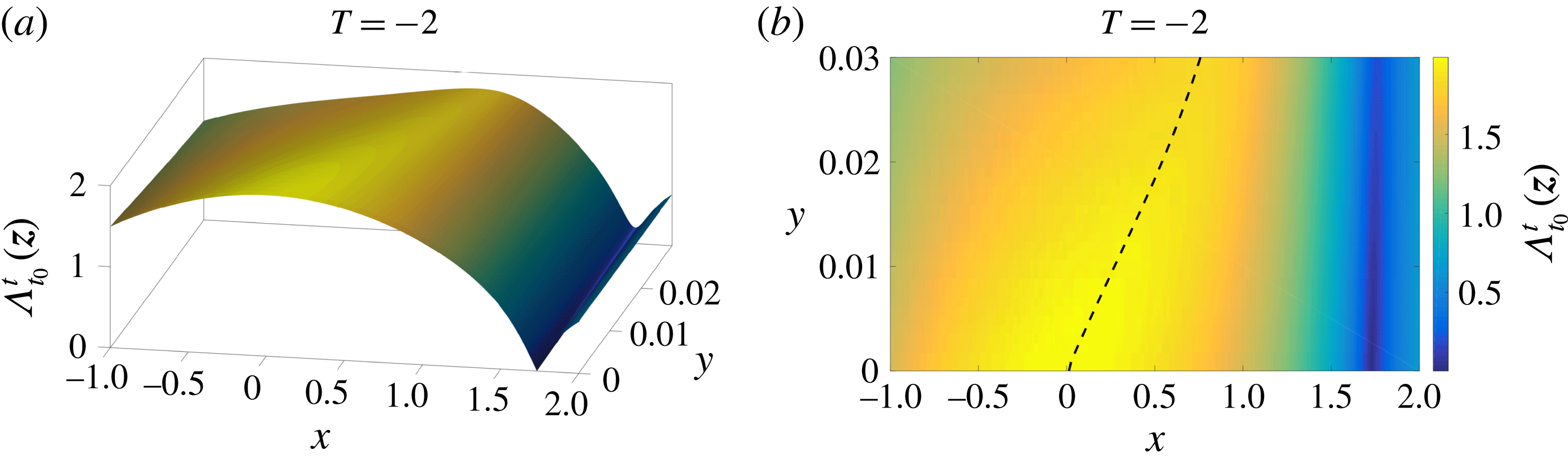
(a) Three-dimensional plot of the backward FTLE field computed for an integration time
 $T=2$
, equal to the extent of the time interval used in figure 7(d). (b) Top view of (a) along with a nearby FTLE ridge shown in dashed black.

Figure 9 shows the backward FTLE computed for an integration time
 $T=2$
, equal to the extent of the time interval used in figure 7(d). Specifically, figure 9(a) shows the three-dimensional plot of the FTLE field, and figure 9(b) the corresponding two-dimensional plot along with the FTLE ridge shown in dashed black. As described in § 2, ridges of the backward FTLE are frequently used diagnostics for the most attracting material lines in the flow, and have already been used to describe flow separation (see, e.g., Garth et al. (Reference Garth, Li, Tricoche, Hansen and Hagen2009), Miron & Vétel (Reference Miron and Vétel2015), Nelson & Jacobs (Reference Nelson and Jacobs2015, Reference Nelson and Jacobs2016)).
Remarkably, the Lagrangian backbone
 ${\mathcal{B}}(t_{0})$
of separation (cf. figure 7
d) remains completely hidden in the FTLE plot. Indeed, even though also the FTLE plot in figure 9(b) admits a ridge emanating from the wall, this ridge has a shape and a basepoint that differ substantially from the backbone profile and the spiking point identified in figure 7(d). This confirms that the material spike formation in flow separation is not a purely stretching-based phenomenon. Rather, it is characterized by an interplay of stretching and rotation, encoded objectively in the curvature field. That said, we generally expect some signature of a material separation onset in the FTLE field.
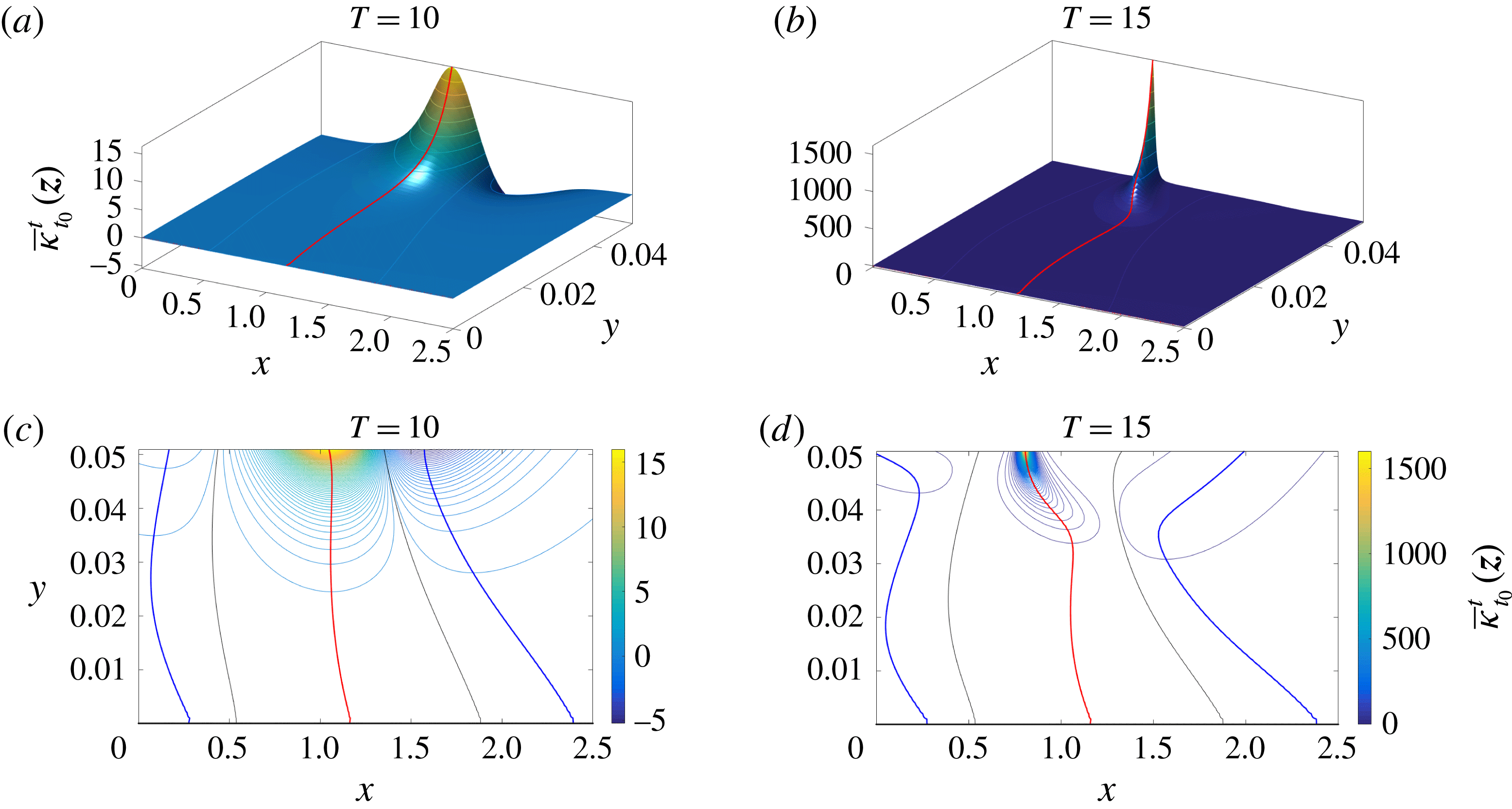
(a) Lagrangian curvature change field
 $\overline{\unicode[STIX]{x1D705}}_{t_{0}}^{t_{0}+T}(\boldsymbol{z})$
for
 $t_{0}=0$
and
 $T=10$
. (b) The same as (a) for
 $T=15$
. (c,d) Contour plots of the scalar fields in (a,b). The red curves show the initial position
 ${\mathcal{B}}(0)$
of the Lagrangian backbone of separation; the blue curves show the sets of minimal signed curvature change in the vicinity of
 ${\mathcal{B}}(0)$
; the black curves represent the zero set of
 $\overline{\unicode[STIX]{x1D705}}_{t_{0}}^{t_{0}+T}(\boldsymbol{z})$
, as sketched in figure 5(b).

6.1.2 Time-periodic flow
Here we consider the moving cylinder flow with
 $\unicode[STIX]{x1D6FA}=5$
,
 $U_{0}=0$
,
 $\unicode[STIX]{x1D6FD}=6$
and
 $\unicode[STIX]{x1D714}_{c}=2\unicode[STIX]{x03C0}$
. These parameter values generate a time-periodic flow with period
 $T_{p}=1$
. Figure 10 shows the
 $t_{0}=0$
positions of the Lagrangian backbone of separation for two different integration times. Panels (a,b) show the Lagrangian curvature change fields
 $\overline{\unicode[STIX]{x1D705}}_{t_{0}}^{t_{0}+T}(\boldsymbol{z})$
for
 $T=10$
and
 $T=15$
. Panels (c,d) show the corresponding contour plots of these two scalar fields. The initial position
 ${\mathcal{B}}(0)$
of the Lagrangian backbone of separation is shown in red; the sets of minimal signed curvature in the vicinity of
 ${\mathcal{B}}(0)$
are shown in blue; the zero set of
 $\overline{\unicode[STIX]{x1D705}}_{t_{0}}^{t_{0}+T}(\boldsymbol{z})$
is shown in black, as sketched in figure 5(b). Similarly to the steady case, for time-periodic flows with period
 $T_{p}$
analysed over a time interval
 $[t_{0},t_{0}+T],~T=nT_{p},~n\in \mathbb{N}^{+}$
, the initial position of the Lagrangian backbone
 ${\mathcal{B}}(0)$
of separation does not depend on
 $t_{0}$
.
Figure 10(c,d) illustrates that the Lagrangian spiking point
 $s_{p}$
is the same when computed over an integer multiple of the flow period
 $T_{p}=1$
(cf. Proposition 2). The shape of the backbone of separation, however, depends on
 $T$
. Similarly to the case of steady flows, the sets of Lagrangian maximum and minimum curvature change connect to the wall at the same locations, as long as
 $T$
is an integer multiple of
 $T_{p}$
, as discussed in appendix D.
Lagrangian backbone
 ${\mathcal{B}}(t)$
of the separation spike (red) extracted from
 $\overline{\unicode[STIX]{x1D705}}_{0}^{15}(\boldsymbol{z})$
(cf. figure 10
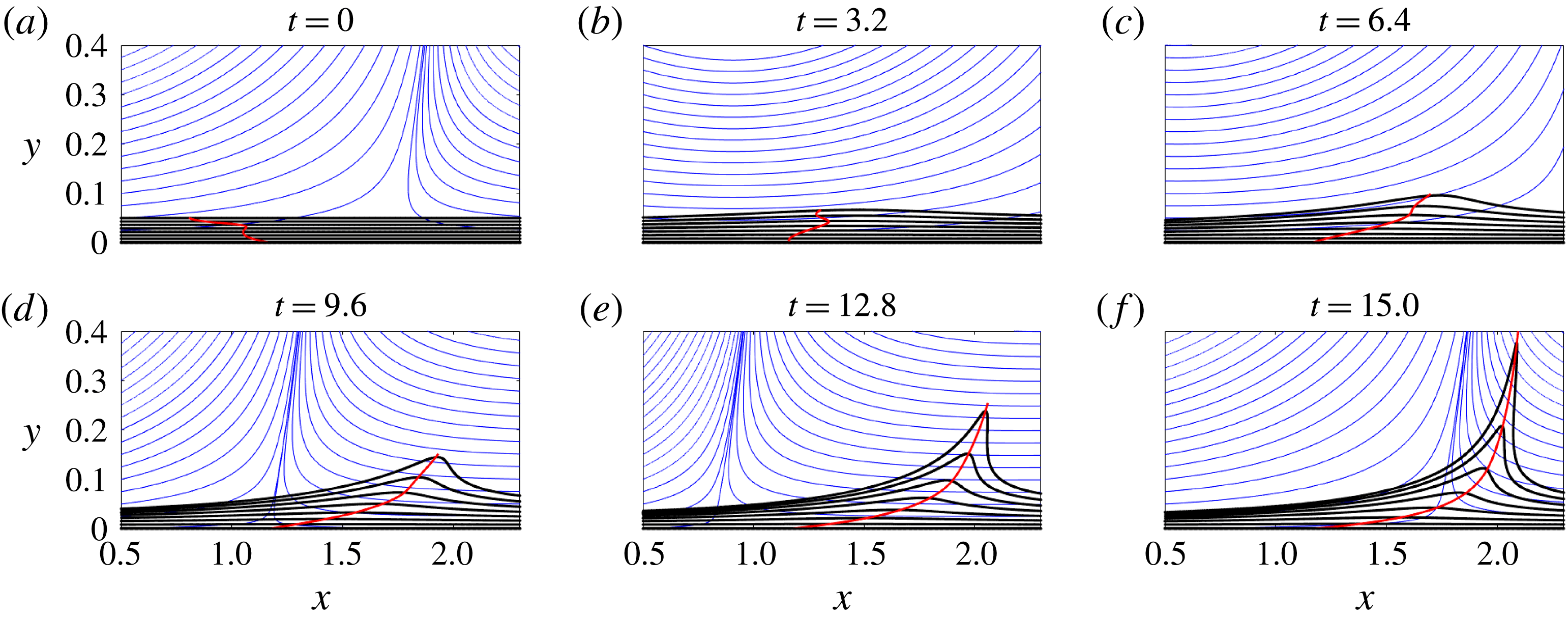
d) at different times, along with the streamlines (blue) and the material lines initially parallel to the wall (black). The full material evolution is available as supplementary movie 5.

Figure 11 shows the Lagrangian backbone
 ${\mathcal{B}}(t)$
of separation extracted from
 $\overline{\unicode[STIX]{x1D705}}_{0}^{15}(\boldsymbol{z})$
(cf. figure 10
d) at different times, along with the streamlines (blue) and the material lines initially parallel to the wall (black). The full material evolution is available as supplementary movie 5. The backbone curve that we locate acts as the theoretical centrepiece of the material spike from its birth to its developed Lagrangian shape.
Figure 11 confirms also that the Prandtl point (i.e. where a singular streamline connects to the wall) is unrelated to flow separation in unsteady flows.
6.2 Time-aperiodic flow
Here, we consider the general time-aperiodic rotating–translating cylinder flow with the parameter values
 $\unicode[STIX]{x1D6FA}=3.5$
,
 $U_{0}=0.3$
,
 $\unicode[STIX]{x1D6FD}=0.5$
and
 $\unicode[STIX]{x1D714}_{c}=2\unicode[STIX]{x03C0}/5$
, which appears to create moving separation. From the classic asymptotic perspective, therefore, separation is believed to be off-wall in this case. Therefore, prior separation criteria seek an off-wall separation point in the flow.
(a) Lagrangian curvature change field
 $\overline{\unicode[STIX]{x1D705}}_{t_{0}}^{t_{0}+T}(\boldsymbol{z})$
for
 $t_{0}=0$
and
 $T=7$
. (b) The same as (a) for
 $T=8$
. (c,d) Contour plots of the scalar fields in (a,b). The red curves show the initial position
 ${\mathcal{B}}(0)$
of the Lagrangian backbone of separation.

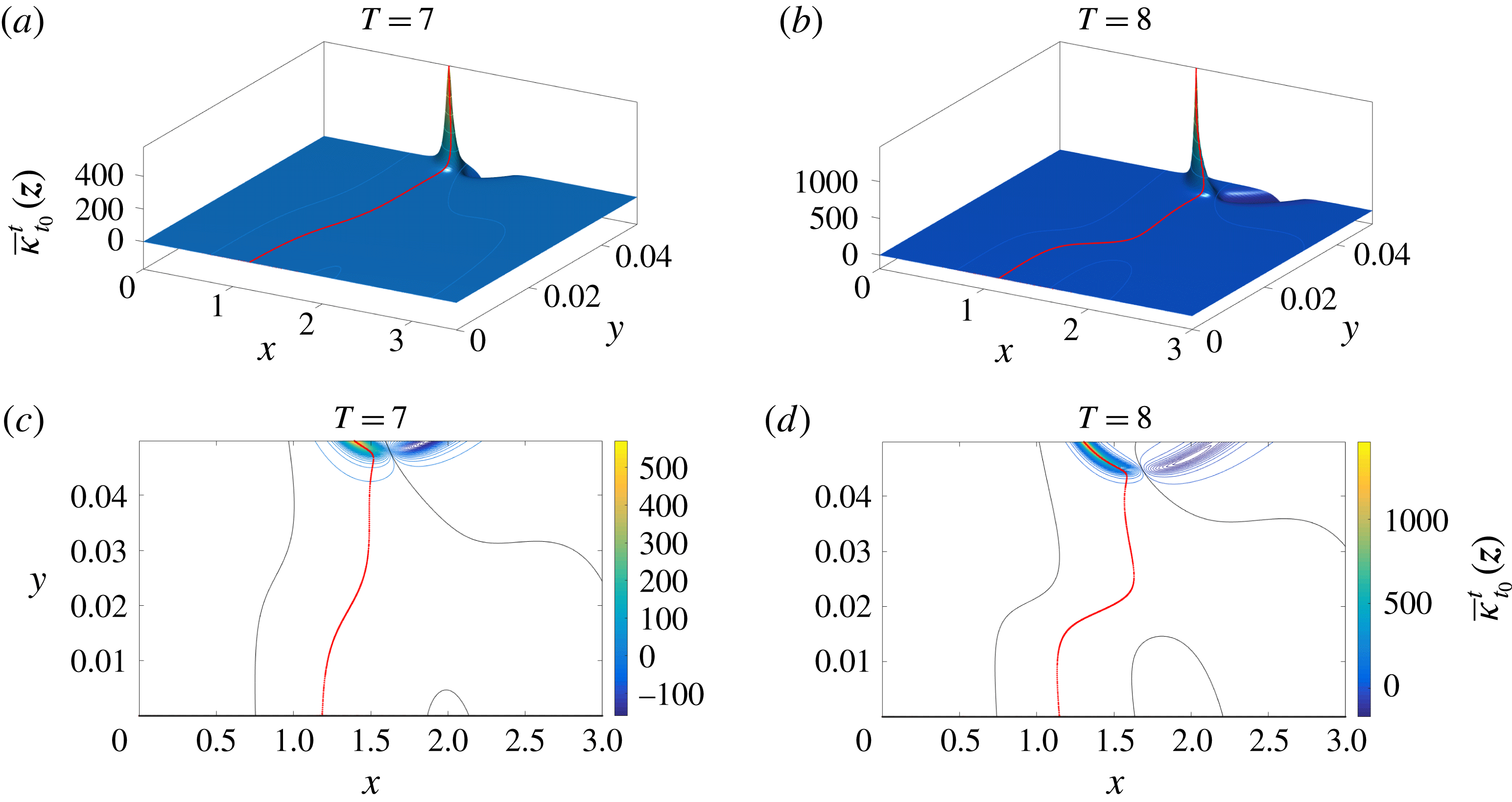
Figure 12 shows the initial position
 ${\mathcal{B}}(t_{0})$
of the Lagrangian backbone of separation for two different integration times. Panels (a,b) show the Lagrangian curvature change fields
 $\overline{\unicode[STIX]{x1D705}}_{t_{0}}^{t_{0}+T}(\boldsymbol{z})$
for
 $t_{0}=0$
,
 $T=7$
and
 $T=8$
. Panels (c,d) show the contours of these two scalar fields. The initial position
 ${\mathcal{B}}(0)$
of the backbone of separation is shown in red and the zero set of
 $\overline{\unicode[STIX]{x1D705}}_{t_{0}}^{t_{0}+T}(\boldsymbol{z})$
is shown in black. Remarkably, the Lagrangian backbone of separation connects to the wall, consistent with the findings of Surana & Haller (Reference Surana and Haller2008) in an appropriate frame, with the Lagrangian spiking point satisfying the formulae in Proposition 2.
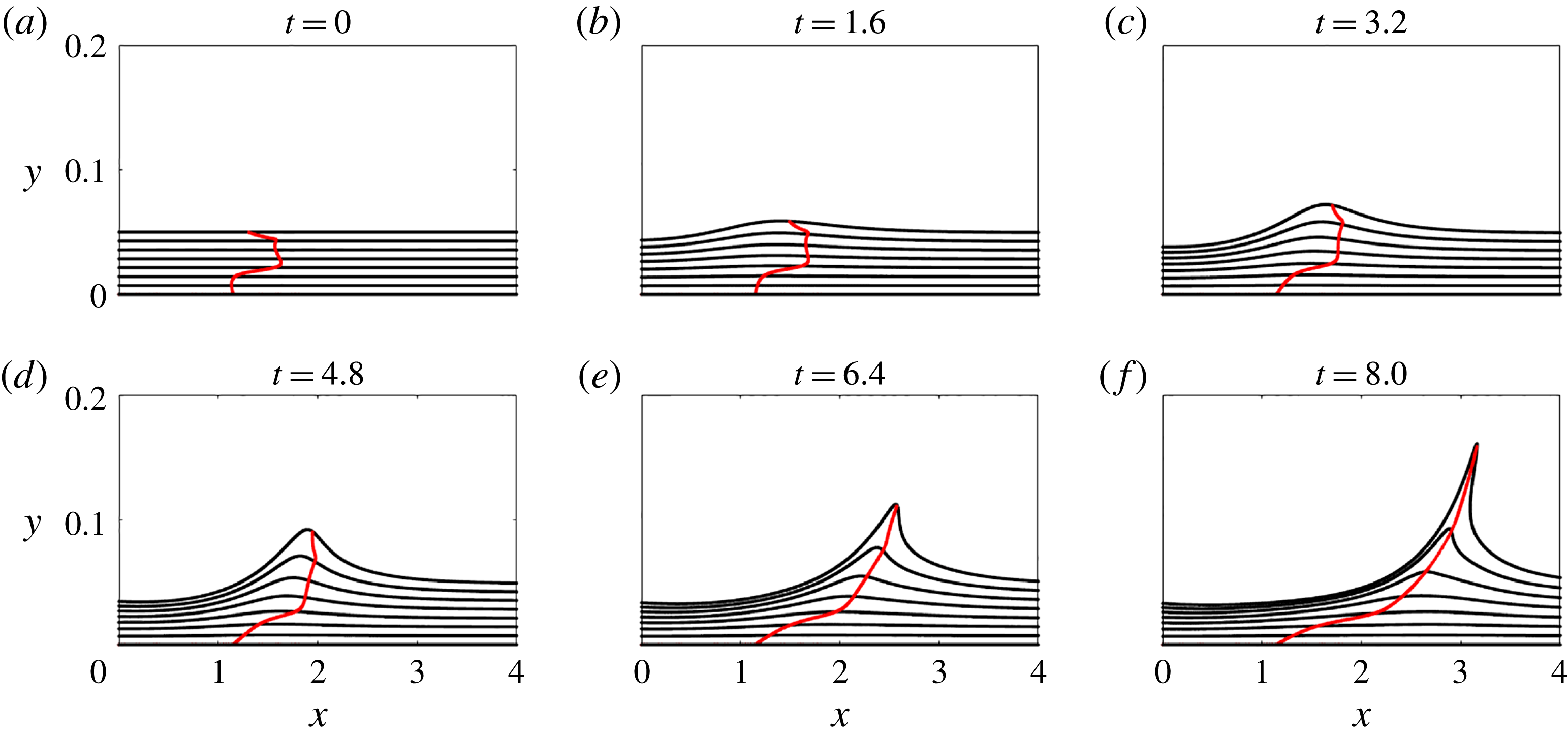
Lagrangian backbone
 ${\mathcal{B}}(t)$
of separation extracted from
 $\overline{\unicode[STIX]{x1D705}}_{0}^{8}(\boldsymbol{z})$
(cf. figure 12
d) at different times, and the material lines initially parallel to the wall (black). The full material evolution is available as supplementary movie 6.

Figure 13 confirms that
 ${\mathcal{B}}(t)$
indeed acts as the evolving centrepiece of a forming material spike. This is the case even though the upwelling in the lower material layers is barely visible yet. The full material evolution is available as supplementary movie 6.
6.2.1 Off-wall perception of separation
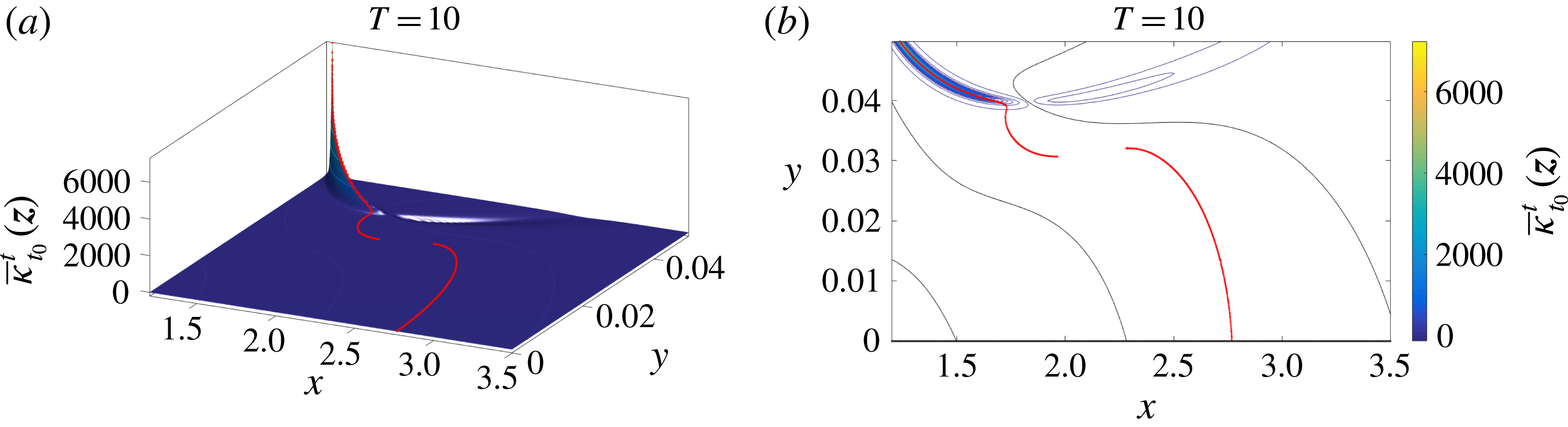
Although we are primarily interested in the birth of separation, rather than its long-term behaviour, we now analyse the same unsteady flow of § 6.2 for a longer time interval. Similarly to figure 12, figure 14 shows the initial position of the Lagrangian backbone of separation extracted from
 $\overline{\unicode[STIX]{x1D705}}_{0}^{10}(\boldsymbol{z})$
. Figure 14(a) shows the Lagrangian curvature change field
 $\overline{\unicode[STIX]{x1D705}}_{0}^{10}(\boldsymbol{z})$
and figure 14(b) shows the contours of the same field along with the initial position
 ${\mathcal{B}}(0)$
of the backbone of separation in red. In contrast to figure 12, for
 $T=10$
, the backbone has two disconnected components, namely an upper part connected to the highest value of
 $\overline{\unicode[STIX]{x1D705}}_{t_{0}}^{t_{0}+T}(\boldsymbol{z})$
and a lower part connected to the wall. This suggests that for this longer time interval, the observed material spike is dominated by an off-wall separation process, which coexists with a more localized upwelling phenomenon at the wall.
The same as figure 12 for larger
 $T$
. (a) Lagrangian curvature change field
 $\overline{\unicode[STIX]{x1D705}}_{t_{0}}^{t_{0}+T}(\boldsymbol{z})$
for
 $T=10$
. (b) Contour plots of the scalar fields in (a). The red curves show the initial position
 ${\mathcal{B}}(0)$
of the Lagrangian backbone of separation.

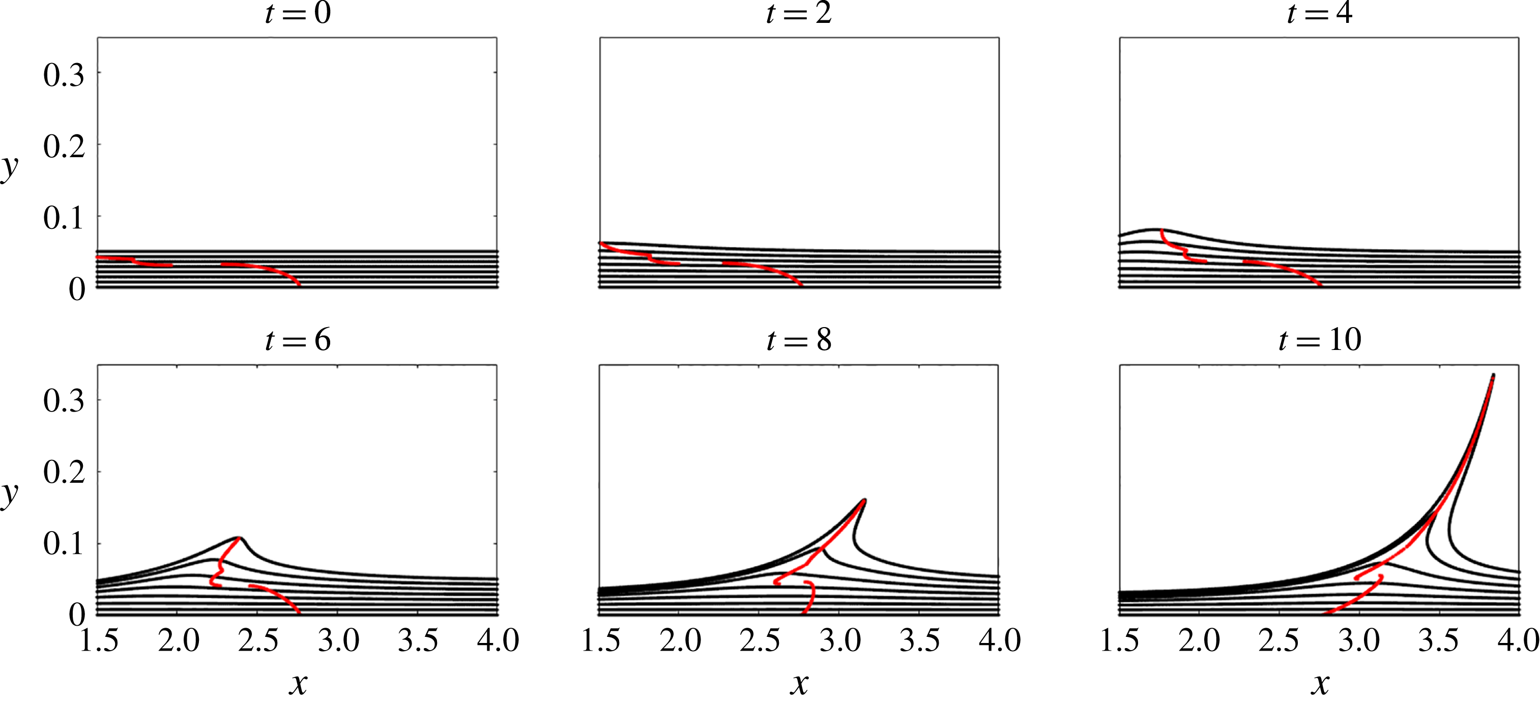
Lagrangian backbone
 ${\mathcal{B}}(t)$
of separation (red) extracted from
 $\overline{\unicode[STIX]{x1D705}}_{0}^{10}(\boldsymbol{z})$
(cf. figure 14
b) at different times, along with the evolution of material lines initially parallel to the wall (black). The full evolution of material lines is available as supplementary movie 7.

This prediction is consistent with figure 15, which shows the evolving Lagrangian backbone
 ${\mathcal{B}}(t)$
at different times in red, along with evolving material lines initially parallel to the wall shown in black. The full material evolution is available as supplementary movie 7.
For shorter observation times, material upwelling starting at the wall can be traced all the way to the tip of the separation spike along a single backbone curve. As
 $T$
increases, a bifurcation takes place in which the local wall-based upwelling decouples from the globally observable spike, whose base point is now off the wall. We emphasize that this result does not rely on a priori heuristic assumptions such as the existence of an off-wall separation point. The presence of an on-wall or off-wall separation, instead, is a result of our theory, encoded in the topology of the Lagrangian backbone of separation.
Previous approaches to unsteady separation would miss this spike structure. In particular, the spike formation criteria of Van Dommelen (Reference Van Dommelen1981) and Van Dommelen & Shen (Reference Van Dommelen and Shen1982) would fail to detect a spike in this example as this flow develops no finite-time singularities. The ghost-manifold-based approach of Surana & Haller (Reference Surana and Haller2008) would also be inapplicable due to the lack of a clear decomposition of the present flow into a slow mean and faster oscillations.
6.3 Flow over a circular cylinder
Here we consider the flow pattern of swirling vortices caused by the flow separation around a circular cylinder, modelled by Jung, Tél & Ziemniak (Reference Jung, Tél and Ziemniak1993). We summarize the details of this flow in appendix H. As in Jung et al. (Reference Jung, Tél and Ziemniak1993), we choose a set of parameters for which the model approximates the Navier–Stokes solution for this geometry with
 $Re\approx 250$
, leading to a time-periodic flow with period
 $T_{p}=1.107$
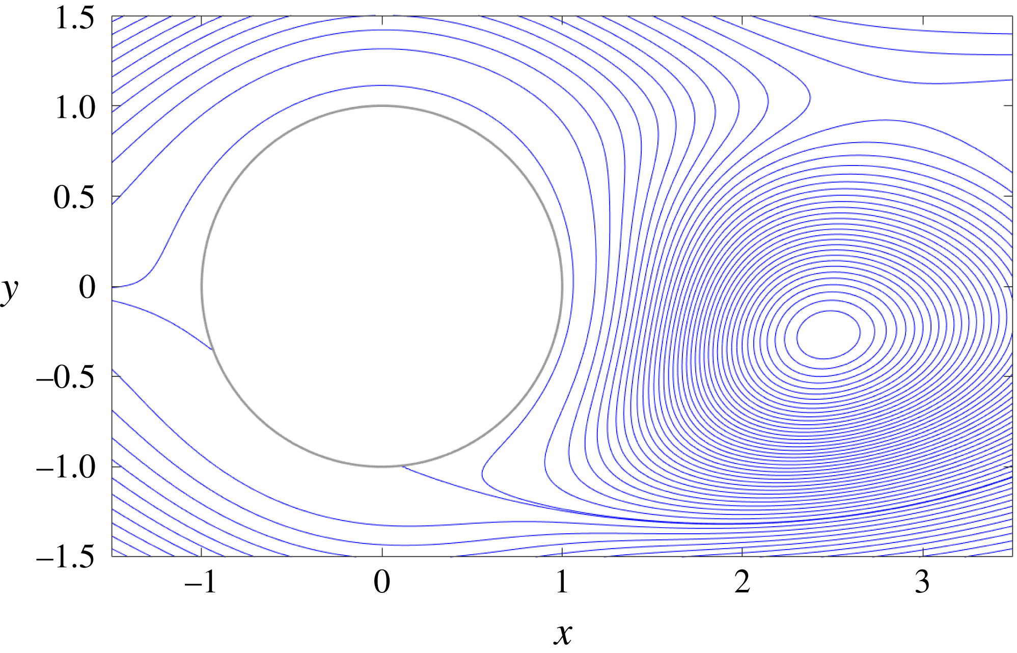
. We show a representative snapshot of the corresponding streamlines in figure 16.
Streamlines of the flow over a circular cylinder at
 $t=0$
.

In the present example, we compute the two highest positive ridges of the Lagrangian curvature change field, showing that our method is able to promptly capture both of the separation profiles present in the flow past a cylinder.
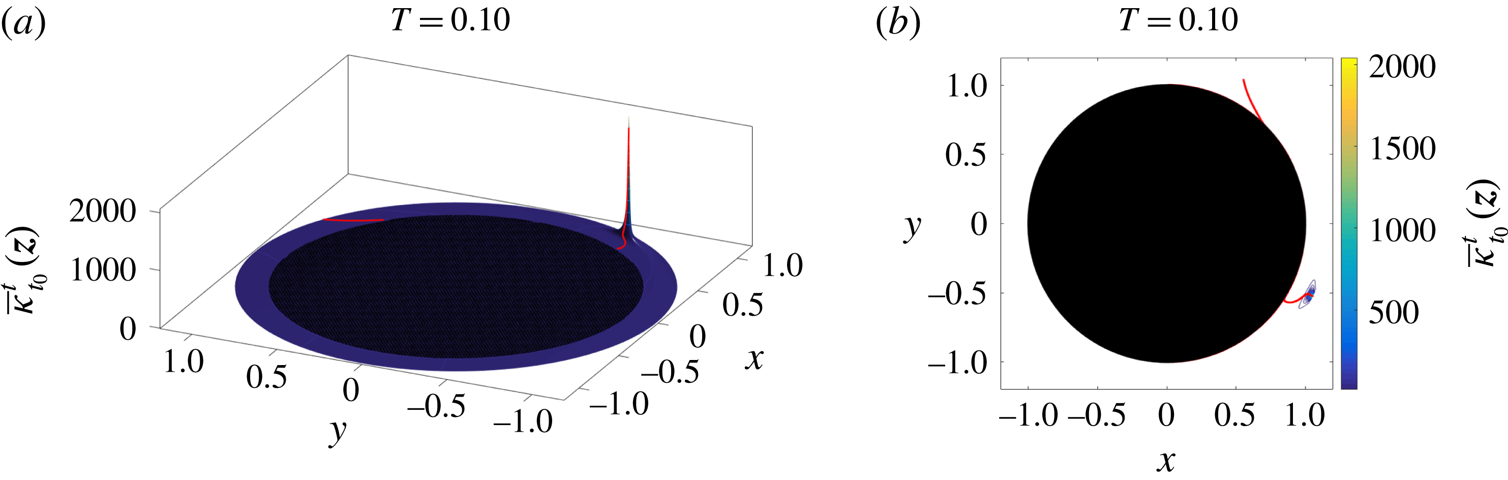
Figure 17 shows the initial positions of the Lagrangian backbones of separation for
 $t_{0}=0$
and
 $T=0.1$
. Specifically, figure 17(a) shows the Lagrangian curvature change field
 $\overline{\unicode[STIX]{x1D705}}_{t_{0}}^{t_{0}+T}(\boldsymbol{z})$
and figure 17(b) shows the contours of
 $\overline{\unicode[STIX]{x1D705}}_{t_{0}}^{t_{0}+T}(\boldsymbol{z})$
, along with the Lagrangian backbones
 ${\mathcal{B}}(0)$
of separation shown in red. Our theory not only identifies both separation profiles, but also objectively distinguishes them through the value of
 $\overline{\unicode[STIX]{x1D705}}_{t_{0}}^{t_{0}+T}(\boldsymbol{z})$
, and hence signals where the spike formation takes place first.
Figure 18 shows in red the Lagrangian backbones
 ${\mathcal{B}}(t)$
of separation extracted from
 $\overline{\unicode[STIX]{x1D705}}_{0}^{0.1}(\boldsymbol{z})$
(cf. figure 17
b) at different times, along with the streamlines (blue) and the material lines initially parallel to the wall (black). The green dot represents the instantaneous Prandtl point (i.e. the zero-skin-friction point) defined by (1.1). The full material evolution is available as supplementary movie 8.
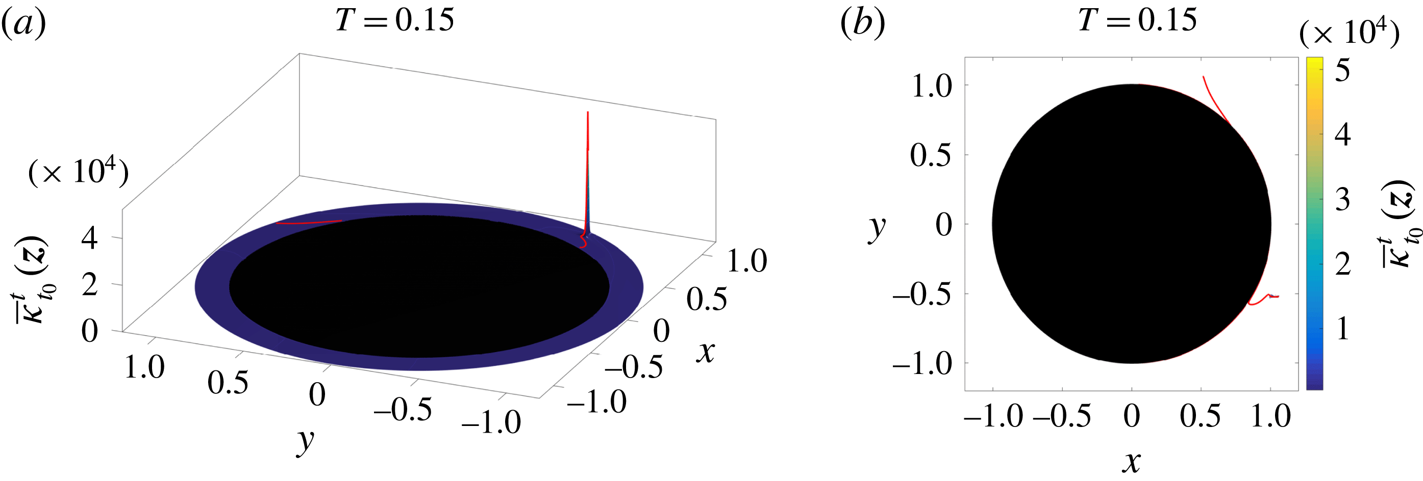
As already observed in the previous examples, figure 18 confirms again that the birth of the material spike is unrelated to the instantaneous Prandtl point. Figures 19 and 20 show the same results as figures 17 and 18 for a longer time interval,
 $T=0.15$
.
(a) Lagrangian curvature change field
 $\overline{\unicode[STIX]{x1D705}}_{t_{0}}^{t_{0}+T}(\boldsymbol{z})$
for
 $t_{0}=0$
and
 $T=0.1$
. (b) Contour plot of
 $\overline{\unicode[STIX]{x1D705}}_{0}^{0.1}$
. The red curves show the initial positions of the Lagrangian backbones
 ${\mathcal{B}}(0)$
of separation.

Lagrangian backbones
 ${\mathcal{B}}(t)$
of separation (red) extracted from
 $\overline{\unicode[STIX]{x1D705}}_{0}^{0.1}(\boldsymbol{z})$
(cf. figure 17
b) at different times, along with the streamlines (blue) and the material lines initially parallel to the cylinder (black). The green dot represents the instantaneous Prandtl point (i.e. zero-skin-friction point) defined by (1.1). The full material evolution is available as supplementary movie 8.

The same as figure 17 but for a longer
 $T=0.15$
. (a) Lagrangian curvature change field
 $\overline{\unicode[STIX]{x1D705}}_{t_{0}}^{t_{0}+T}(\boldsymbol{z})$
for
 $T=0.15$
. (b) Contour plots of
 $\overline{\unicode[STIX]{x1D705}}_{0}^{0.15}$
. The red curves show the initial positions of the Lagrangian backbones
 ${\mathcal{B}}(t_{0})$
of separation.

The same as figure 18 but for a longer
 $T=0.15$
. Lagrangian backbones
 ${\mathcal{B}}(t)$
of separation (red) extracted from
 $\overline{\unicode[STIX]{x1D705}}_{0}^{0.15}(\boldsymbol{z})$
(cf. figure 19
b) at different times, along with the streamlines (blue) and the material lines initially parallel to the cylinder (black). The green dot represents the instantaneous Prandtl point defined by (1.1). The full material evolution is available as supplementary movie 9.

We observe that although the time intervals considered here,
 $T=0.1$
and
 $T=0.15$
, are significantly shorter than one period of the flow,
 $T_{p}=1.107$
, our theory still accurately uncovers the backbones of separation spikes. Unlike available long-term (Miron & Vétel Reference Miron and Vétel2015) and asymptotic (Haller Reference Haller2004) Lagrangian separation theories, our theory does not need velocity information over a full period of the flow in order to locate spike formation.
6.4 Experimental time-aperiodic flow: separation induced by a rotating and translating cylinder
In this section, we apply our results to an unsteady dataset obtained from an experimental set-up similar to that of Weldon et al. (Reference Weldon, Peacock, Jacobs, Helu and Haller2008). A horizontal cylinder rotates and translates parallel to a wall of a transparent tank filled with glycerin, as shown in figure 21. A particle image velocimetry (PIV) technique is used in a horizontal plane to measure the two velocity components in a region where the flow is approximately two-dimensional. For the case considered here, the cylinder radius is
 $R_{c}=1.27$
cm, the cylinder rotation velocity is
 $\unicode[STIX]{x1D6FA}=60$
rpm, its translation velocity is
 $U_{c}=U_{0}+\unicode[STIX]{x1D6FD}\cos (\unicode[STIX]{x1D714}_{c}t)$
, with
 $U_{0}=1~\text{cm}~\text{s}^{-1}$
,
 $\unicode[STIX]{x1D6FD}=8~\text{cm}~\text{s}^{-1}$
and
 $\unicode[STIX]{x1D714}_{c}=\unicode[STIX]{x03C0}~\text{rad}~\text{s}^{-1}$
, and the initial position of the cylinder is at
 $x_{c_{0}}=7.5$
cm,
 $y_{c}=y_{c_{0}}=5.75$
cm.
Experimental set-up.

The velocity field is available over a time interval
 $t\in [0~\text{s},3~\text{s}]$
every
 $1/15$
s on a uniform spatial grid bounded by
 $x\in [-0.5~\text{cm},12.5~\text{cm}]$
and
 $y\in [0~\text{cm},10~\text{cm}]$
, with a grid size of
 $0.08$
cm in both directions.
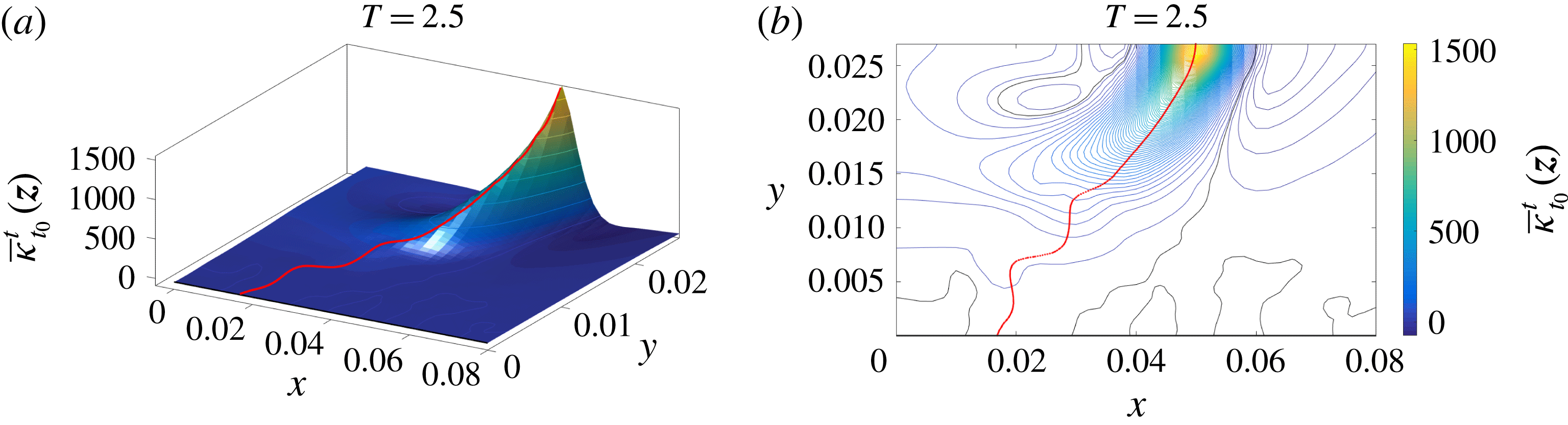
Figure 22 shows the initial position of the Lagrangian backbone
 ${\mathcal{B}}(t_{0})$
of separation extracted from
 $\overline{\unicode[STIX]{x1D705}}_{t_{0}}^{T}(\boldsymbol{z})$
for
 $t_{0}=0~\text{s},~T=2.5~\text{s}$
. Specifically, figure 22(a) shows the Lagrangian curvature change field
 $\overline{\unicode[STIX]{x1D705}}_{t_{0}}^{t_{0}+T}(\boldsymbol{z})$
and figure 22(b) shows the contours of
 $\overline{\unicode[STIX]{x1D705}}_{t_{0}}^{t_{0}+T}(\boldsymbol{z})$
along with the Lagrangian backbone
 ${\mathcal{B}}(0)$
of separation in red.
(a) Lagrangian curvature change field
 $\overline{\unicode[STIX]{x1D705}}_{t_{0}}^{t_{0}+T}(\boldsymbol{z})$
for
 $t_{0}=0$
and
 $T=2.5$
s. (b) Contours of the scalar fields in (a). The red curve shows the initial position
 ${\mathcal{B}}(t_{0})$
of the Lagrangian backbone of separation.

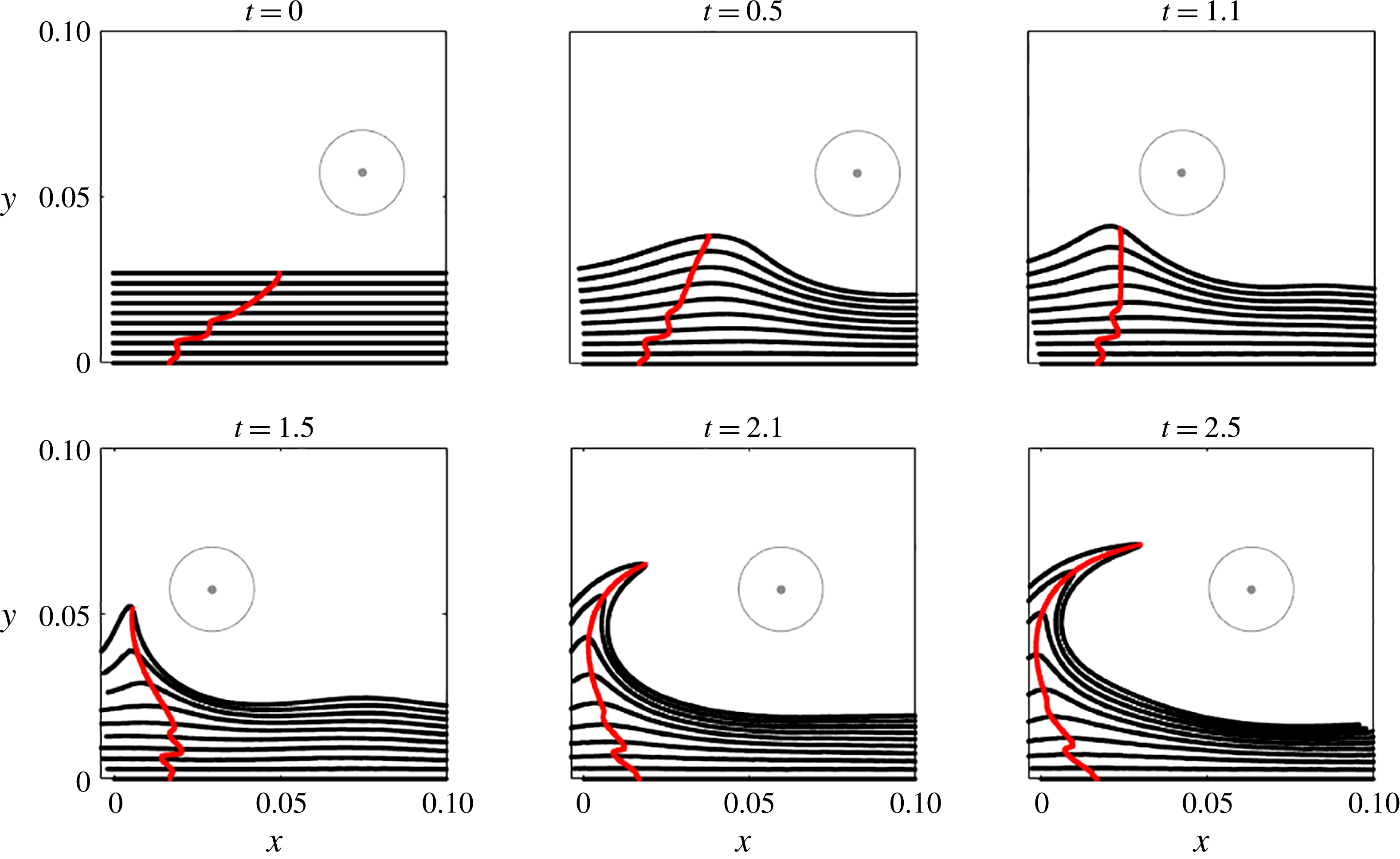
Lagrangian backbone
 ${\mathcal{B}}(t)$
of separation (red) extracted from
 $\overline{\unicode[STIX]{x1D705}}_{0}^{2.5}(\boldsymbol{z})$
(cf. figure 22
b) at different times, along with the material lines initially parallel to the wall (black). The full evolution of the material lines is available as supplementary movie 10.

As we have already noted in § 6.2, while this flow setting separation is generally believed to generate off-wall separation, the Lagrangian backbone still connects to the wall. Figure 23 shows snapshots of the corresponding material evolution in the separation process. The full material evolution is available as supplementary movie 10.
7 Conclusions
We have developed a frame-independent theory of material spike formation during flow separation over a no-slip boundary in two-dimensional flows with arbitrary time dependence. Based on the curvature evolution of material lines, our theory uncovers the centrepiece of the material spike from its birth to its fully developed Lagrangian structure.
Curvature objectively combines stretching- and rotation-based kinematic quantities, and hence reveals flow features that remain hidden to criteria based only on stretching or rotation. As a byproduct, we have derived analytical formulae for the Lagrangian curvature evolution and the instantaneous curvature rate along a material line that is advected under a general compressible flow. Our purely kinematic theory can be applied to arbitrary numerical, experimental or model velocity fields.
We have also identified a previously undetected spiking point where the backbone of a material spike connects to the boundary. We have shown that this spiking point can be computed from averaged wall-based quantities. Remarkably, even in steady flows, the spiking point differs from the classic Prandtl separation point. Although in the aerodynamic community the spike formation has generally been associated exclusively with unsteady separation (Van Dommelen Reference Van Dommelen1981; Van Dommelen & Shen Reference Van Dommelen and Shen1982), here we have shown that the same phenomenon exists also in steady flows. This underlines the fact that material spike formation is a universal phenomenon that is unrelated to the time dependence of the flow and to the presence of singularities in the flow.
Similarly to the asymptotic Lagrangian definition of the separation point (Haller Reference Haller2004), the spiking point identified here is constant in steady flows and in time-periodic flows analysed over a time interval that is a multiple of their period, while it moves in general unsteady flows. Our backbone of separation, instead, evolves materially under all flow conditions, serving as the core of the separating spike. Our theory is effective also over short time intervals and admits a rigorous instantaneous limit. These properties, inaccessible to existing criteria, make the present approach promising for monitoring and controlling separation.
We have also illustrated how our curvature-based approach explains the perception of off-wall separation in unsteady flows, and provided conditions under which such a perception is justified. Specifically, we have found that for a relatively short time interval
 $T$
, the backbone of separation consists of a single connected component joining the off-wall portion of the material spike to the spiking point. For longer
 $T$
, instead, the backbone bifurcates into two disconnected components: one passing through the off-wall region characterized by the highest curvature change and the other one connected to the wall at the new spiking point location. This suggests that for longer
 $T$
, the Lagrangian spike is driven by off-wall dynamics, losing its connection with its original on-wall signature. This analysis offers a way to identify the limiting
 $T$
at which transition from on-wall to off-wall separation occurs.
Supplementary movies
Supplementary movies are available at https://doi.org/10.1017/jfm.2018.206.
Appendix A. Proof of Theorem 1
Here we derive a formula for the time evolution of curvature and curvature rate along a material curve
 $\unicode[STIX]{x1D6FE}$
advected under the flow map
 $\unicode[STIX]{x1D641}_{t_{0}}^{t}$
. We denote the parametrization of
 $\unicode[STIX]{x1D6FE}$
at the initial time by
 $\boldsymbol{r}(s)$
,
 $s\in [s_{1},s_{2}]$
, and its local tangent vector by
 $\boldsymbol{r}^{\prime }(s):=\text{d}\boldsymbol{r}/\text{d}s$
.
A.1 Curvature along a material curve
Substituting (3.1) and (3.3) into (3.4), we obtain the following expression for the curvature of
 $\unicode[STIX]{x1D6FE}$
advected by the flow
 $\unicode[STIX]{x1D641}_{t_{0}}^{t}$
:
 $$\begin{eqnarray}\unicode[STIX]{x1D705}_{t_{0}}^{t}(s)=\frac{\langle \tilde{\boldsymbol{r}}^{\prime \prime }(s),\unicode[STIX]{x1D64D}\unicode[STIX]{x1D735}\unicode[STIX]{x1D641}_{t_{0}}^{t}(\boldsymbol{r}(s))\boldsymbol{r}^{\prime }(s)\rangle }{\langle \boldsymbol{r}^{\prime }(s),\unicode[STIX]{x1D63E}_{t_{0}}^{t}(\boldsymbol{r}(s))\boldsymbol{r}^{\prime }(s)\rangle }.\end{eqnarray}$$
The only missing quantity for the evaluation of
 $\unicode[STIX]{x1D705}_{t_{0}}^{t}(s)$
is the term
 $\tilde{\boldsymbol{r}}^{\prime \prime }$
. Differentiation of (3.1) with respect to
 $s$
gives
 $$\begin{eqnarray}\tilde{r}_{i}^{\prime \prime }(s)=p_{1_{i}}(s)+p_{2_{i}}(s),\quad i\in \{1,2\},\end{eqnarray}$$
where
 $$\begin{eqnarray}\left.\begin{array}{@{}l@{}}\displaystyle p_{1_{i}}=\frac{\unicode[STIX]{x1D735}\unicode[STIX]{x1D641}_{{t_{0}}_{ij,n}}^{t}\boldsymbol{r}_{n}^{\prime }\boldsymbol{r}_{j}^{\prime }+\unicode[STIX]{x1D735}\unicode[STIX]{x1D641}_{{t_{0}}_{ip}}^{t}\boldsymbol{r}_{p}^{\prime \prime }}{\sqrt{\boldsymbol{r}_{k}^{\prime }\unicode[STIX]{x1D63E}_{{t_{0}}_{km}}^{t}\boldsymbol{r}_{m}^{\prime }}},\\ \displaystyle p_{2_{i}}=-\frac{\unicode[STIX]{x1D735}\unicode[STIX]{x1D641}_{{t_{0}}_{ij}}^{t}\boldsymbol{r}_{j}^{\prime }[2\unicode[STIX]{x1D63E}_{{t_{0}}_{pq}}^{t}\boldsymbol{r}_{p}^{\prime }\boldsymbol{r}_{q}^{\prime \prime }+\boldsymbol{r}_{l}^{\prime }\unicode[STIX]{x1D63E}_{{t_{0}}_{ln,h}}^{t}\boldsymbol{r}_{n}^{\prime }\boldsymbol{r}_{h}^{\prime }]}{2(\boldsymbol{r}_{k}^{\prime }(s)\unicode[STIX]{x1D63E}_{{t_{0}}_{km}}^{t}(s)\boldsymbol{r}_{m}^{\prime }(s))^{3/2}}.\end{array}\right\}\end{eqnarray}$$
In (A 3), as well as in the rest of the paper, summation is implied over repeated indices, all of the indices vary from 1 to 2, and commas in subscripts denote partial differentiation, i.e.
 $\unicode[STIX]{x1D61B}_{ij,k}(\boldsymbol{z}):=\unicode[STIX]{x2202}_{\boldsymbol{z}_{k}}\unicode[STIX]{x1D61B}_{ij}(\boldsymbol{z})$
, where
 $\unicode[STIX]{x1D61B}$
denotes a two-dimensional tensor field. Substituting (A 2)–(A 3) into (A 1), we obtain
 $$\begin{eqnarray}\unicode[STIX]{x1D705}_{t_{0}}^{t}(s)=\frac{\langle \,\boldsymbol{p}_{1}(s)+\boldsymbol{p}_{2}(s),\unicode[STIX]{x1D64D}\unicode[STIX]{x1D735}\unicode[STIX]{x1D641}_{t_{0}}^{t}(\boldsymbol{r}(s))\boldsymbol{r}^{\prime }(s)\rangle }{\langle \boldsymbol{r}^{\prime }(s),\unicode[STIX]{x1D63E}_{t_{0}}^{t}(\boldsymbol{r}(s))\boldsymbol{r}^{\prime }(s)\rangle }=\unicode[STIX]{x1D705}_{1}(s)+\unicode[STIX]{x1D705}_{2}(s)-\unicode[STIX]{x1D705}_{3}(s)-\unicode[STIX]{x1D705}_{4}(s),\end{eqnarray}$$
where, dropping the dependence on
 $s$
,
 $$\begin{eqnarray}\left.\begin{array}{@{}l@{}}\displaystyle \unicode[STIX]{x1D705}_{1}=\frac{\unicode[STIX]{x1D735}\unicode[STIX]{x1D641}_{{t_{0}}_{ij,n}}^{t}\boldsymbol{r}_{n}^{\prime }\boldsymbol{r}_{j}^{\prime }\unicode[STIX]{x1D619}_{il}\unicode[STIX]{x1D735}\unicode[STIX]{x1D641}_{{t_{0}}_{lp}}^{t}\boldsymbol{r}_{p}^{\prime }}{(\boldsymbol{r}_{k}^{\prime }\unicode[STIX]{x1D63E}_{{t_{0}}_{km}}^{t}\boldsymbol{r}_{m}^{\prime })^{3/2}},\\ \displaystyle \unicode[STIX]{x1D705}_{2}=\frac{\unicode[STIX]{x1D735}\unicode[STIX]{x1D641}_{{t_{0}}_{ij}}^{t}\boldsymbol{r}_{j}^{\prime \prime }\unicode[STIX]{x1D619}_{il}\unicode[STIX]{x1D735}\unicode[STIX]{x1D641}_{{t_{0}}_{lp}}^{t}\boldsymbol{r}_{p}^{\prime }}{(\boldsymbol{r}_{k}^{\prime }\unicode[STIX]{x1D63E}_{{t_{0}}_{km}}^{t}\boldsymbol{r}_{m}^{\prime })^{3/2}},\\ \displaystyle \unicode[STIX]{x1D705}_{3}=\frac{\unicode[STIX]{x1D735}\unicode[STIX]{x1D641}_{{t_{0}}_{ij}}^{t}\boldsymbol{r}_{j}^{\prime }\unicode[STIX]{x1D619}_{il}\unicode[STIX]{x1D735}\unicode[STIX]{x1D641}_{{t_{0}}_{ln}}^{t}\boldsymbol{r}_{n}^{\prime }A}{(\boldsymbol{r}_{k}^{\prime }\unicode[STIX]{x1D63E}_{{t_{0}}_{km}}^{t}\boldsymbol{r}_{m}^{\prime })^{5/2}},\quad A=\boldsymbol{r}_{k}^{\prime }\unicode[STIX]{x1D63E}_{{t_{0}}_{km}}^{t}\boldsymbol{r}_{m}^{\prime \prime },\\ \displaystyle \unicode[STIX]{x1D705}_{4}=\frac{\unicode[STIX]{x1D735}\unicode[STIX]{x1D641}_{{t_{0}}_{ij}}^{t}\boldsymbol{r}_{j}^{\prime }\unicode[STIX]{x1D619}_{il}\unicode[STIX]{x1D735}\unicode[STIX]{x1D641}_{{t_{0}}_{lp}}^{t}\boldsymbol{r}_{p}^{\prime }B}{2(\boldsymbol{r}_{k}^{\prime }\unicode[STIX]{x1D63E}_{{t_{0}}_{km}}^{t}\boldsymbol{r}_{m}^{\prime })^{5/2}},\quad B=\boldsymbol{r}_{l}^{\prime }\unicode[STIX]{x1D63E}_{{t_{0}}_{ln,h}}^{t}\boldsymbol{r}_{n}^{\prime }\boldsymbol{r}_{h}^{\prime }.\end{array}\right\}\end{eqnarray}$$
It should be noted that
 $\unicode[STIX]{x1D735}\unicode[STIX]{x1D641}_{{t_{0}}_{ij}}^{t}\boldsymbol{r}_{j}^{\prime }\unicode[STIX]{x1D619}_{il}\unicode[STIX]{x1D735}\unicode[STIX]{x1D641}_{{t_{0}}_{ln}}^{t}\boldsymbol{r}_{n}^{\prime }\equiv \langle \unicode[STIX]{x1D735}\unicode[STIX]{x1D641}_{t_{0}}^{t}\boldsymbol{r}^{\prime },\unicode[STIX]{x1D64D}\unicode[STIX]{x1D735}\unicode[STIX]{x1D641}_{t_{0}}^{t}\boldsymbol{r}^{\prime }\rangle \equiv 0$
and hence
 $\unicode[STIX]{x1D705}_{3}=\unicode[STIX]{x1D705}_{4}\equiv 0$
. Therefore, we rewrite (A 4) in compact form as
 $$\begin{eqnarray}\unicode[STIX]{x1D705}_{t_{0}}^{t}=\frac{\langle (\unicode[STIX]{x1D735}^{2}\unicode[STIX]{x1D641}_{t_{0}}^{t}(\boldsymbol{r})\boldsymbol{r}^{\prime })\boldsymbol{r}^{\prime },\unicode[STIX]{x1D64D}\unicode[STIX]{x1D735}\unicode[STIX]{x1D641}_{t_{0}}^{t}(\boldsymbol{r})\boldsymbol{r}^{\prime }\rangle }{\langle \boldsymbol{r}^{\prime },\unicode[STIX]{x1D63E}_{t_{0}}^{t}(\boldsymbol{r})\boldsymbol{r}^{\prime }\rangle ^{3/2}}+\frac{\langle \unicode[STIX]{x1D735}\unicode[STIX]{x1D641}_{t_{0}}^{t}(\boldsymbol{r})\boldsymbol{r}^{\prime \prime },\unicode[STIX]{x1D64D}\unicode[STIX]{x1D735}\unicode[STIX]{x1D641}_{t_{0}}^{t}(\boldsymbol{r})\boldsymbol{r}^{\prime }\rangle }{\langle \boldsymbol{r}^{\prime },\unicode[STIX]{x1D63E}_{t_{0}}^{t}(\boldsymbol{r})\boldsymbol{r}^{\prime }\rangle ^{3/2}}=\unicode[STIX]{x1D705}_{1}+\unicode[STIX]{x1D705}_{2},\end{eqnarray}$$
where
 $(\unicode[STIX]{x1D735}^{2}\unicode[STIX]{x1D641}_{t_{0}}^{t}(\boldsymbol{r})\boldsymbol{r}^{\prime })_{ij}:=\unicode[STIX]{x1D641}_{{t_{0}}_{i,jk}}^{t}(\boldsymbol{r})\boldsymbol{r}_{k}^{\prime }$
. By denoting the components of
 $\boldsymbol{r}^{\prime \prime }$
along the directions
 $\boldsymbol{r}^{\prime }/|\boldsymbol{r}^{\prime }|$
and
 $\unicode[STIX]{x1D64D}\boldsymbol{r}^{\prime }/|\boldsymbol{r}^{\prime }|$
by
 $\boldsymbol{r}_{\Vert }^{\prime \prime }$
and
 $\boldsymbol{r}_{\bot }^{\prime \prime }$
respectively, and observing that
 $\langle \unicode[STIX]{x1D735}\unicode[STIX]{x1D641}_{t_{0}}^{t}(\boldsymbol{r})\boldsymbol{r}_{\Vert }^{\prime \prime },\unicode[STIX]{x1D64D}\unicode[STIX]{x1D735}\unicode[STIX]{x1D641}_{t_{0}}^{t}(\boldsymbol{r})\boldsymbol{r}^{\prime }\rangle =0$
, the expression for
 $\unicode[STIX]{x1D705}_{2}$
simplifies to
 $$\begin{eqnarray}\displaystyle \unicode[STIX]{x1D705}_{2} & = & \displaystyle \frac{\langle \unicode[STIX]{x1D735}\unicode[STIX]{x1D641}_{t_{0}}^{t}(\boldsymbol{r})\boldsymbol{r}_{\bot }^{\prime \prime },\unicode[STIX]{x1D64D}\unicode[STIX]{x1D735}\unicode[STIX]{x1D641}_{t_{0}}^{t}(\boldsymbol{r})\boldsymbol{r}^{\prime }\rangle }{\langle \boldsymbol{r}^{\prime },\unicode[STIX]{x1D63E}_{t_{0}}^{t}(\boldsymbol{r})\boldsymbol{r}^{\prime }\rangle ^{3/2}}\nonumber\\ \displaystyle & = & \displaystyle \frac{\langle \boldsymbol{r}^{\prime \prime },\unicode[STIX]{x1D64D}\boldsymbol{r}^{\prime }\rangle }{|\boldsymbol{r}^{\prime }|^{2}}\frac{\langle \unicode[STIX]{x1D735}\unicode[STIX]{x1D641}_{t_{0}}^{t}(\boldsymbol{r})\unicode[STIX]{x1D64D}\boldsymbol{r}^{\prime },\unicode[STIX]{x1D64D}\unicode[STIX]{x1D735}\unicode[STIX]{x1D641}_{t_{0}}^{t}(\boldsymbol{r})\boldsymbol{r}^{\prime }\rangle }{\langle \boldsymbol{r}^{\prime },\unicode[STIX]{x1D63E}_{t_{0}}^{t}(\boldsymbol{r})\boldsymbol{r}^{\prime }\rangle ^{3/2}}\nonumber\\ \displaystyle & = & \displaystyle \frac{\langle \boldsymbol{r}^{\prime \prime },\unicode[STIX]{x1D64D}\boldsymbol{r}^{\prime }\rangle }{|\boldsymbol{r}^{\prime }|^{2}}\frac{\det [\unicode[STIX]{x1D735}\unicode[STIX]{x1D641}_{t_{0}}^{t}(\boldsymbol{r})]|\boldsymbol{r}^{\prime }|^{2}}{\langle \boldsymbol{r}^{\prime },\unicode[STIX]{x1D63E}_{t_{0}}^{t}(\boldsymbol{r})\boldsymbol{r}^{\prime }\rangle ^{3/2}}\nonumber\\ \displaystyle & = & \displaystyle \frac{\langle \boldsymbol{r}^{\prime \prime },\unicode[STIX]{x1D64D}\boldsymbol{r}^{\prime }\rangle \det [\unicode[STIX]{x1D735}\unicode[STIX]{x1D641}_{t_{0}}^{t}(\boldsymbol{r})]}{\langle \boldsymbol{r}^{\prime },\unicode[STIX]{x1D63E}_{t_{0}}^{t}(\boldsymbol{r})\boldsymbol{r}^{\prime }\rangle ^{3/2}}.\end{eqnarray}$$
The final formula for
 $\unicode[STIX]{x1D705}_{t_{0}}^{t}$
is then given by
 $$\begin{eqnarray}\unicode[STIX]{x1D705}_{t_{0}}^{t}=\frac{\langle (\unicode[STIX]{x1D735}^{2}\unicode[STIX]{x1D641}_{t_{0}}^{t}(\boldsymbol{r})\boldsymbol{r}^{\prime })\boldsymbol{r}^{\prime },\unicode[STIX]{x1D64D}\unicode[STIX]{x1D735}\unicode[STIX]{x1D641}_{t_{0}}^{t}(\boldsymbol{r})\boldsymbol{r}^{\prime }\rangle }{\langle \boldsymbol{r}^{\prime },\unicode[STIX]{x1D63E}_{t_{0}}^{t}(\boldsymbol{r})\boldsymbol{r}^{\prime }\rangle ^{3/2}}+\frac{\langle \boldsymbol{r}^{\prime \prime },\unicode[STIX]{x1D64D}\boldsymbol{r}^{\prime }\rangle \det [\unicode[STIX]{x1D735}\unicode[STIX]{x1D641}_{t_{0}}^{t}(\boldsymbol{r})]}{\langle \boldsymbol{r}^{\prime },\unicode[STIX]{x1D63E}_{t_{0}}^{t}(\boldsymbol{r})\boldsymbol{r}^{\prime }\rangle ^{3/2}},\end{eqnarray}$$
which can be also rewritten as
 $$\begin{eqnarray}\unicode[STIX]{x1D705}_{t_{0}}^{t}=\frac{\langle (\unicode[STIX]{x1D735}^{2}\unicode[STIX]{x1D641}_{t_{0}}^{t}(\boldsymbol{r})\boldsymbol{r}^{\prime })\boldsymbol{r}^{\prime },\unicode[STIX]{x1D64D}\unicode[STIX]{x1D735}\unicode[STIX]{x1D641}_{t_{0}}^{t}(\boldsymbol{r})\boldsymbol{r}^{\prime }\rangle }{\langle \boldsymbol{r}^{\prime },\unicode[STIX]{x1D63E}_{t_{0}}^{t}(\boldsymbol{r})\boldsymbol{r}^{\prime }\rangle ^{3/2}}+\unicode[STIX]{x1D705}_{0}\det [\unicode[STIX]{x1D735}\unicode[STIX]{x1D641}_{t_{0}}^{t}(\boldsymbol{r})]\left(\frac{\langle \boldsymbol{r}^{\prime },\boldsymbol{r}^{\prime }\rangle }{\langle \boldsymbol{r}^{\prime },\unicode[STIX]{x1D63E}_{t_{0}}^{t}(\boldsymbol{r})\boldsymbol{r}^{\prime }\rangle }\right)^{3/2},\end{eqnarray}$$
where
 $\unicode[STIX]{x1D705}_{0}:=\unicode[STIX]{x1D705}_{t_{0}}^{t_{0}}$
denotes the curvature of
 $\unicode[STIX]{x1D6FE}$
at time
 $t_{0}$
. In the case of arclength parametrization of
 $\unicode[STIX]{x1D6FE}$
(i.e.
 $\langle \boldsymbol{r}^{\prime },\boldsymbol{r}^{\prime }\rangle \equiv 1$
), and of incompressible flows (i.e.
 $\unicode[STIX]{x1D735}\boldsymbol{\cdot }\boldsymbol{f}\equiv 0$
,
 $\det [\unicode[STIX]{x1D735}\unicode[STIX]{x1D641}_{t_{0}}^{t}]\equiv 1$
), (A 9) simplifies to
 $$\begin{eqnarray}\unicode[STIX]{x1D705}_{t_{0}}^{t}=\frac{\langle (\unicode[STIX]{x1D735}^{2}\unicode[STIX]{x1D641}_{t_{0}}^{t}(\boldsymbol{r})\boldsymbol{r}^{\prime })\boldsymbol{r}^{\prime },\unicode[STIX]{x1D64D}\unicode[STIX]{x1D735}\unicode[STIX]{x1D641}_{t_{0}}^{t}(\boldsymbol{r})\boldsymbol{r}^{\prime }\rangle }{\langle \boldsymbol{r}^{\prime },\unicode[STIX]{x1D63E}_{t_{0}}^{t}(\boldsymbol{r})\boldsymbol{r}^{\prime }\rangle ^{3/2}}+\frac{\unicode[STIX]{x1D705}_{0}}{\langle \boldsymbol{r}^{\prime },\unicode[STIX]{x1D63E}_{t_{0}}^{t}(\boldsymbol{r})\boldsymbol{r}^{\prime }\rangle ^{3/2}}.\end{eqnarray}$$
A.2 Curvature rate along a material curve
By differentiating (A 8) with respect to time (
 $(\text{d}/\text{d}t)(\cdot ):=\dot{(\cdot )}$
) and evaluating it at
 $t=t_{0}$
, we obtain
 $$\begin{eqnarray}\dot{\unicode[STIX]{x1D705}}_{t_{0}}(s)=\dot{\unicode[STIX]{x1D705}}_{1}(s,t_{0})+\dot{\unicode[STIX]{x1D705}}_{2}(s,t_{0}),\end{eqnarray}$$
where
 $$\begin{eqnarray}\displaystyle \dot{\unicode[STIX]{x1D705}}_{1} & = & \displaystyle \left.\frac{\dot{\overline{\unicode[STIX]{x1D735}\unicode[STIX]{x1D641}_{{t_{0}}_{ij,n}}^{t}}}\boldsymbol{r}_{n}^{\prime }\boldsymbol{r}_{j}^{\prime }\unicode[STIX]{x1D619}_{il}\unicode[STIX]{x1D735}\unicode[STIX]{x1D641}_{{t_{0}}_{lp}}^{t}\boldsymbol{r}_{p}^{\prime }+\unicode[STIX]{x1D735}\unicode[STIX]{x1D641}_{{t_{0}}_{ij,n}}^{t}\boldsymbol{r}_{n}^{\prime }\boldsymbol{r}_{j}^{\prime }\unicode[STIX]{x1D619}_{il}\dot{\overline{\unicode[STIX]{x1D735}\unicode[STIX]{x1D641}_{{t_{0}}_{lp}}^{t}}}\boldsymbol{r}_{p}^{\prime }}{(\boldsymbol{r}_{k}^{\prime }\unicode[STIX]{x1D63E}_{{t_{0}}_{km}}^{t}\boldsymbol{r}_{m}^{\prime })^{3/2}}\right|_{t=t_{0}}\nonumber\\ \displaystyle & & \displaystyle -\,\left.\frac{(\unicode[STIX]{x1D735}\unicode[STIX]{x1D641}_{{t_{0}}_{ij,n}}^{t}\boldsymbol{r}_{n}^{\prime }\boldsymbol{r}_{j}^{\prime }\unicode[STIX]{x1D619}_{il}\unicode[STIX]{x1D735}\unicode[STIX]{x1D641}_{{t_{0}}_{lp}}^{t}\boldsymbol{r}_{p}^{\prime })3\boldsymbol{r}_{n}^{\prime }\dot{\overline{\unicode[STIX]{x1D63E}_{{t_{0}}_{nj}}^{t}}}\boldsymbol{r}_{j}^{\prime }}{2(\boldsymbol{r}_{k}^{\prime }\unicode[STIX]{x1D63E}_{{t_{0}}_{km}}^{t}\boldsymbol{r}_{m}^{\prime })^{5/2}}\right|_{t=t_{0}}\nonumber\\ \displaystyle & = & \displaystyle \frac{\unicode[STIX]{x1D735}\boldsymbol{f}_{ij,n}(t_{0})\boldsymbol{r}_{n}^{\prime }\boldsymbol{r}_{j}^{\prime }\unicode[STIX]{x1D619}_{il}\boldsymbol{r}_{l}^{\prime }}{(\boldsymbol{r}_{k}^{\prime }\boldsymbol{r}_{k}^{\prime })^{3/2}}\nonumber\\ \displaystyle & = & \displaystyle \frac{\langle (\unicode[STIX]{x1D6FB}^{2}\boldsymbol{f}(t_{0})\boldsymbol{r}^{\prime })\boldsymbol{r}^{\prime },\unicode[STIX]{x1D64D}\boldsymbol{r}^{\prime }\rangle }{\langle \boldsymbol{r}^{\prime },\boldsymbol{r}^{\prime }\rangle ^{3/2}},\end{eqnarray}$$
 $$\begin{eqnarray}\displaystyle \dot{\unicode[STIX]{x1D705}}_{2} & = & \displaystyle \left.\frac{\boldsymbol{r}_{i}^{\prime \prime }\unicode[STIX]{x1D619}_{ip}\boldsymbol{r}_{p}^{\prime }\dot{\overline{\det [\unicode[STIX]{x1D735}\unicode[STIX]{x1D641}_{t_{0}}^{t}]}}}{(\boldsymbol{r}_{k}^{\prime }\unicode[STIX]{x1D63E}_{{t_{0}}_{km}}^{t}\boldsymbol{r}_{m}^{\prime })^{3/2}}\right|_{t=t_{0}}-\left.\frac{3\boldsymbol{r}_{i}^{\prime \prime }\unicode[STIX]{x1D619}_{ip}\boldsymbol{r}_{p}^{\prime }\det [\unicode[STIX]{x1D735}\unicode[STIX]{x1D641}_{t_{0}}^{t}]\boldsymbol{r}_{n}^{\prime }\dot{\overline{\unicode[STIX]{x1D63E}_{{t_{0}}_{nj}}^{t}}}\boldsymbol{r}_{j}^{\prime }}{2(\boldsymbol{r}_{k}^{\prime }\unicode[STIX]{x1D63E}_{{t_{0}}_{km}}^{t}\boldsymbol{r}_{m}^{\prime })^{5/2}}\right|_{t=t_{0}}\nonumber\\ \displaystyle & = & \displaystyle \frac{\boldsymbol{r}_{i}^{\prime \prime }\unicode[STIX]{x1D619}_{ip}\boldsymbol{r}_{p}^{\prime }\unicode[STIX]{x1D735}\boldsymbol{\cdot }\boldsymbol{f}(t_{0})}{(\boldsymbol{r}_{k}^{\prime }\boldsymbol{r}_{k}^{\prime })^{3/2}}-\frac{3\boldsymbol{r}_{i}^{\prime \prime }\unicode[STIX]{x1D619}_{ip}\boldsymbol{r}_{p}^{\prime }\boldsymbol{r}_{n}^{\prime }2\unicode[STIX]{x1D61A}_{nj}(t_{0})\boldsymbol{r}_{j}^{\prime }}{2(\boldsymbol{r}_{k}^{\prime }\boldsymbol{r}_{k}^{\prime })^{5/2}}\nonumber\\ \displaystyle & = & \displaystyle \unicode[STIX]{x1D705}_{0}\unicode[STIX]{x1D735}\boldsymbol{\cdot }\boldsymbol{f}(t_{0})-3\unicode[STIX]{x1D705}_{0}\frac{\boldsymbol{r}_{n}^{\prime }\unicode[STIX]{x1D61A}_{nj}(t_{0})\boldsymbol{r}_{j}^{\prime }}{(\boldsymbol{r}_{k}^{\prime }\boldsymbol{r}_{k}^{\prime })}\nonumber\\ \displaystyle & = & \displaystyle \unicode[STIX]{x1D705}_{0}\left[\unicode[STIX]{x1D735}\boldsymbol{\cdot }\boldsymbol{f}(t_{0})-3\frac{\langle \boldsymbol{r}^{\prime },\unicode[STIX]{x1D64E}(t_{0})\boldsymbol{r}^{\prime }\rangle }{\langle \boldsymbol{r}^{\prime },\boldsymbol{r}^{\prime }\rangle }\right].\end{eqnarray}$$
 $$\begin{eqnarray}\left.\begin{array}{@{}c@{}}\displaystyle \dot{\overline{\unicode[STIX]{x1D735}\unicode[STIX]{x1D641}_{{t_{0}}_{ij,k}}^{t}}}|_{t=t_{0}}=\unicode[STIX]{x1D735}\boldsymbol{f}_{ij,k}(t_{0}),\quad \unicode[STIX]{x1D735}\unicode[STIX]{x1D641}_{{t_{0}}_{ij,k}}^{t_{0}}=0,\quad \unicode[STIX]{x1D735}\unicode[STIX]{x1D641}_{{t_{0}}_{ij}}^{t_{0}}\equiv \unicode[STIX]{x1D6FF}_{ij},\\ \displaystyle \dot{\overline{\unicode[STIX]{x1D63E}_{{t_{0}}_{ij}}^{t}}}|_{t=t_{0}}=2\unicode[STIX]{x1D61A}_{ij}(t_{0}),\quad \dot{\overline{\det [\unicode[STIX]{x1D735}\unicode[STIX]{x1D641}_{t_{0}}^{t}]}}|_{t=t_{0}}=\unicode[STIX]{x1D735}\boldsymbol{\cdot }\boldsymbol{f}(t_{0}),\quad \forall i,j,k\in \{1,2\},\end{array}\right\}\end{eqnarray}$$
where
 $\unicode[STIX]{x1D6FF}_{ij}$
is the Kronecker delta. Using the velocity gradient decomposition defined in (2.2)–(2.3), we rewrite
 $\dot{\unicode[STIX]{x1D705}}_{1}$
as
 $$\begin{eqnarray}\displaystyle \dot{\unicode[STIX]{x1D705}}_{1} & = & \displaystyle \frac{[\unicode[STIX]{x1D61A}_{ij,n}(t_{0})+\unicode[STIX]{x1D61E}_{ij,n}(t_{0})]\boldsymbol{r}_{n}^{\prime }\boldsymbol{r}_{j}^{\prime }\unicode[STIX]{x1D619}_{il}\boldsymbol{r}_{l}^{\prime }}{(\boldsymbol{r}_{k}^{\prime }\boldsymbol{r}_{k}^{\prime })^{3/2}}\nonumber\\ \displaystyle & = & \displaystyle \frac{\unicode[STIX]{x1D61A}_{ij,n}(t_{0})\boldsymbol{r}_{n}^{\prime }\boldsymbol{r}_{j}^{\prime }\unicode[STIX]{x1D619}_{il}\boldsymbol{r}_{l}^{\prime }-\frac{1}{2}\unicode[STIX]{x1D735}\unicode[STIX]{x1D714}_{l}(t_{0})\boldsymbol{r}_{l}^{\prime }\unicode[STIX]{x1D619}_{ij}\boldsymbol{r}_{j}^{\prime }\unicode[STIX]{x1D619}_{il}\boldsymbol{r}_{l}^{\prime }}{(\boldsymbol{r}_{k}^{\prime }\boldsymbol{r}_{k}^{\prime })^{3/2}}\nonumber\\ \displaystyle & = & \displaystyle \frac{\langle (\unicode[STIX]{x1D735}\unicode[STIX]{x1D64E}(t_{0})\boldsymbol{r}^{\prime })\boldsymbol{r}^{\prime },\unicode[STIX]{x1D64D}\boldsymbol{r}^{\prime }\rangle }{\langle \boldsymbol{r}^{\prime },\boldsymbol{r}^{\prime }\rangle ^{3/2}}-\frac{\langle \unicode[STIX]{x1D735}\unicode[STIX]{x1D714}(t_{0}),\boldsymbol{r}^{\prime }\rangle }{2\langle \boldsymbol{r}^{\prime },\boldsymbol{r}^{\prime }\rangle ^{1/2}}.\end{eqnarray}$$
Substituting (A 12) and (A 14) into (A 11), we obtain the final formula for the instantaneous curvature rate along
 $\unicode[STIX]{x1D6FE}$
,
 $$\begin{eqnarray}\dot{\unicode[STIX]{x1D705}}_{t_{0}}=\frac{\langle (\unicode[STIX]{x1D735}\unicode[STIX]{x1D64E}(\boldsymbol{r},t_{0})\boldsymbol{r}^{\prime })\boldsymbol{r}^{\prime },\unicode[STIX]{x1D64D}\boldsymbol{r}^{\prime }\rangle }{\langle \boldsymbol{r}^{\prime },\boldsymbol{r}^{\prime }\rangle ^{3/2}}-\frac{\langle \unicode[STIX]{x1D735}\unicode[STIX]{x1D714}(\boldsymbol{r},t_{0}),\boldsymbol{r}^{\prime }\rangle }{2\langle \boldsymbol{r}^{\prime },\boldsymbol{r}^{\prime }\rangle ^{1/2}}+\unicode[STIX]{x1D705}_{0}\left[\unicode[STIX]{x1D735}\boldsymbol{\cdot }\boldsymbol{f}(\boldsymbol{r},t_{0})-3\frac{\langle \boldsymbol{r}^{\prime },\unicode[STIX]{x1D64E}(\boldsymbol{r},t_{0})\boldsymbol{r}^{\prime }\rangle }{\langle \boldsymbol{r}^{\prime },\boldsymbol{r}^{\prime }\rangle }\right].\end{eqnarray}$$
If
 $\boldsymbol{r}(s)$
is the arclength parametrization of
 $\unicode[STIX]{x1D6FE}$
and the flow is incompressible, (A 15) simplifies to
 $$\begin{eqnarray}\dot{\unicode[STIX]{x1D705}}_{t_{0}}=\langle (\unicode[STIX]{x1D735}\unicode[STIX]{x1D64E}(\boldsymbol{r},t_{0})\boldsymbol{r}^{\prime })\boldsymbol{r}^{\prime },\unicode[STIX]{x1D64D}\boldsymbol{r}^{\prime }\rangle -{\textstyle \frac{1}{2}}\langle \unicode[STIX]{x1D735}\unicode[STIX]{x1D714}(\boldsymbol{r},t_{0}),\boldsymbol{r}^{\prime }\rangle -3\unicode[STIX]{x1D705}_{0}\langle \boldsymbol{r}^{\prime },\unicode[STIX]{x1D64E}(\boldsymbol{r},t_{0})\boldsymbol{r}^{\prime }\rangle .\end{eqnarray}$$
Appendix B. Identities to compute
$\unicode[STIX]{x1D705}_{t_{0}}^{t}$
without taking spatial derivatives of
$\unicode[STIX]{x1D641}_{t_{0}}^{t}$
numerically


Here we derive an alternative formula for the computation of
 $\unicode[STIX]{x1D705}_{t_{0}}^{t}(\unicode[STIX]{x1D6FE})$
(cf. (3.6)) that does not require the computation of spatial derivatives of
 $\unicode[STIX]{x1D641}_{t_{0}}^{t}$
numerically, which is usually a sensitive procedure. Dropping the spatial dependence on
 $s$
, we rewrite the initial value problem governing the curvature evolution along
 $\unicode[STIX]{x1D6FE}$
as
 $$\begin{eqnarray}\left.\begin{array}{@{}c@{}}\dot{\unicode[STIX]{x1D705}}_{t}=\underbrace{\left[\unicode[STIX]{x1D735}\boldsymbol{\cdot }\boldsymbol{f}(\boldsymbol{r}_{t},t)-3\frac{\langle \boldsymbol{r}_{t}^{\prime },\unicode[STIX]{x1D64E}(\boldsymbol{r}_{t},t)\boldsymbol{r}_{t}^{\prime }\rangle }{\langle \boldsymbol{r}_{t}^{\prime },\boldsymbol{r}_{t}^{\prime }\rangle }\right]}_{a(t)}\unicode[STIX]{x1D705}_{t}+\underbrace{\frac{\langle \unicode[STIX]{x1D64D}\boldsymbol{r}_{t}^{\prime },(\unicode[STIX]{x1D735}\unicode[STIX]{x1D64E}(\boldsymbol{r}_{t},t)\boldsymbol{r}_{t}^{\prime })\boldsymbol{r}_{t}^{\prime }\rangle }{\langle \boldsymbol{r}_{t}^{\prime },\boldsymbol{r}_{t}^{\prime }\rangle ^{3/2}}-\frac{\langle \unicode[STIX]{x1D735}\unicode[STIX]{x1D714}(\boldsymbol{r}_{t},t),\boldsymbol{r}_{t}^{\prime }\rangle }{2\langle \boldsymbol{r}_{t}^{\prime },\boldsymbol{r}_{t}^{\prime }\rangle ^{1/2}}}_{\boldsymbol{b}(t)},\\ \boldsymbol{r}_{t}=\unicode[STIX]{x1D641}_{t_{0}}^{t}(\boldsymbol{r}),\\ \boldsymbol{r}_{t}^{\prime }=\unicode[STIX]{x1D735}\unicode[STIX]{x1D641}_{t_{0}}^{t}(\boldsymbol{r})\boldsymbol{r}^{\prime },\\ \unicode[STIX]{x1D705}_{t_{0}}=\unicode[STIX]{x1D705}_{0},\end{array}\right\}\end{eqnarray}$$
which, by the variation of constants formula (Arnold Reference Arnold1973), admits the solution
 $$\begin{eqnarray}\unicode[STIX]{x1D705}_{t_{0}}^{t}=\unicode[STIX]{x1D705}_{0}\exp \left(\int _{t_{0}}^{t}a(\unicode[STIX]{x1D70F})\,\text{d}\unicode[STIX]{x1D70F}\right)+\exp \left(\int _{t_{0}}^{t}a(\unicode[STIX]{x1D70F})\,\text{d}\unicode[STIX]{x1D70F}\right)\int _{t_{0}}^{t}\boldsymbol{b}(\unicode[STIX]{x1D70F})\exp \left(-\int _{t_{0}}^{\unicode[STIX]{x1D70F}}a(\tilde{\unicode[STIX]{x1D70F}})\,\text{d}\tilde{\unicode[STIX]{x1D70F}}\right)\,\text{d}\unicode[STIX]{x1D70F}.\end{eqnarray}$$
We recall that the gradient of the flow map
 $\unicode[STIX]{x1D735}\unicode[STIX]{x1D641}_{t_{0}}^{t}$
is the fundamental matrix solution of the equation of variations
 $$\begin{eqnarray}\dot{\overline{\unicode[STIX]{x1D735}\unicode[STIX]{x1D641}_{t_{0}}^{t}}}(\boldsymbol{z}_{0})=\unicode[STIX]{x1D735}\boldsymbol{f}(\unicode[STIX]{x1D641}_{t_{0}}^{t}(\boldsymbol{z}_{0}),t)\unicode[STIX]{x1D735}\unicode[STIX]{x1D641}_{t_{0}}^{t}(\boldsymbol{z}_{0}).\end{eqnarray}$$
By Liouville’s theorem (Arnold Reference Arnold1973),
 $\unicode[STIX]{x1D735}\unicode[STIX]{x1D641}_{t_{0}}^{t}$
satisfies the relationship
 $$\begin{eqnarray}\det \unicode[STIX]{x1D735}\unicode[STIX]{x1D641}_{t_{0}}^{t}(\boldsymbol{z}_{0})=\exp \left(\int _{t_{0}}^{t}\unicode[STIX]{x1D735}\boldsymbol{\cdot }\boldsymbol{f}(\unicode[STIX]{x1D641}_{t_{0}}^{\unicode[STIX]{x1D70F}}(\boldsymbol{z}_{0}),\unicode[STIX]{x1D70F})\,\text{d}\unicode[STIX]{x1D70F}\right).\end{eqnarray}$$
By comparing (3.6) and (B 2), and using (B 1) and (B 4), we obtain the following identities:
 $$\begin{eqnarray}\displaystyle \left.\begin{array}{@{}l@{}}\displaystyle \frac{\langle \boldsymbol{r}^{\prime },\unicode[STIX]{x1D63E}_{t_{0}}^{t}(\boldsymbol{r})\boldsymbol{r}^{\prime }\rangle }{\langle \boldsymbol{r}^{\prime },\boldsymbol{r}^{\prime }\rangle }=\exp \left(2\int _{t_{0}}^{t}\frac{\langle \boldsymbol{r}_{\unicode[STIX]{x1D70F}}^{\prime },\unicode[STIX]{x1D64E}(\boldsymbol{r}_{\unicode[STIX]{x1D70F}},\unicode[STIX]{x1D70F})\boldsymbol{r}_{\unicode[STIX]{x1D70F}}^{\prime }\rangle }{\langle \boldsymbol{r}_{\unicode[STIX]{x1D70F}}^{\prime },\boldsymbol{r}_{\unicode[STIX]{x1D70F}}^{\prime }\rangle }\,\text{d}\unicode[STIX]{x1D70F}\right),\\ \displaystyle \frac{\langle (\unicode[STIX]{x1D735}^{2}\unicode[STIX]{x1D641}_{t_{0}}^{t}\boldsymbol{r}^{\prime })\boldsymbol{r}^{\prime },\unicode[STIX]{x1D64D}\unicode[STIX]{x1D735}\unicode[STIX]{x1D641}_{t_{0}}^{t}\boldsymbol{r}^{\prime }\rangle }{\langle \boldsymbol{r}^{\prime },\unicode[STIX]{x1D63E}_{t_{0}}^{t}(\boldsymbol{r})\boldsymbol{r}^{\prime }\rangle ^{3/2}}=\exp \left(\int _{t_{0}}^{t}\unicode[STIX]{x1D735}\boldsymbol{\cdot }\boldsymbol{f}(\boldsymbol{r}_{\unicode[STIX]{x1D70F}},\unicode[STIX]{x1D70F})-3\frac{\langle \boldsymbol{r}_{\unicode[STIX]{x1D70F}}^{\prime },\unicode[STIX]{x1D64E}(\boldsymbol{r}_{\unicode[STIX]{x1D70F}},\unicode[STIX]{x1D70F})\boldsymbol{r}_{\unicode[STIX]{x1D70F}}^{\prime }\rangle }{\langle \boldsymbol{r}_{\unicode[STIX]{x1D70F}}^{\prime },\boldsymbol{r}_{\unicode[STIX]{x1D70F}}^{\prime }\rangle }\,\text{d}\unicode[STIX]{x1D70F}\right)\\ \displaystyle \quad \qquad \times \,\int _{t_{0}}^{t}\left[\frac{\langle \unicode[STIX]{x1D64D}\boldsymbol{r}_{\unicode[STIX]{x1D70F}}^{\prime },(\unicode[STIX]{x1D735}\unicode[STIX]{x1D64E}(\boldsymbol{r}_{\unicode[STIX]{x1D70F}},\unicode[STIX]{x1D70F})\boldsymbol{r}_{\unicode[STIX]{x1D70F}}^{\prime })\boldsymbol{r}_{\unicode[STIX]{x1D70F}}^{\prime }\rangle }{\langle \boldsymbol{r}_{\unicode[STIX]{x1D70F}}^{\prime },\boldsymbol{r}_{\unicode[STIX]{x1D70F}}^{\prime }\rangle ^{3/2}}-\frac{\langle \unicode[STIX]{x1D735}\unicode[STIX]{x1D714}(\boldsymbol{r}_{\unicode[STIX]{x1D70F}},\unicode[STIX]{x1D70F}),\boldsymbol{r}_{\unicode[STIX]{x1D70F}}^{\prime }\rangle }{2\langle \boldsymbol{r}_{\unicode[STIX]{x1D70F}}^{\prime },\boldsymbol{r}_{\unicode[STIX]{x1D70F}}^{\prime }\rangle ^{1/2}}\right]\\ \displaystyle \quad \qquad \times \,\exp \left(-\int _{t_{0}}^{\unicode[STIX]{x1D70F}}\unicode[STIX]{x1D735}\boldsymbol{\cdot }\boldsymbol{f}(\boldsymbol{r}_{\unicode[STIX]{x1D716}},\unicode[STIX]{x1D716})-3\frac{\langle \boldsymbol{r}_{\unicode[STIX]{x1D716}}^{\prime },\unicode[STIX]{x1D64E}(\boldsymbol{r}_{\unicode[STIX]{x1D716}},\unicode[STIX]{x1D716})\boldsymbol{r}_{\unicode[STIX]{x1D716}}^{\prime }\rangle }{\langle \boldsymbol{r}_{\unicode[STIX]{x1D716}}^{\prime },\boldsymbol{r}_{\unicode[STIX]{x1D716}}^{\prime }\rangle }\,\text{d}\unicode[STIX]{x1D716}\right)\,\text{d}\unicode[STIX]{x1D70F}.\end{array}\right\} & & \displaystyle\end{eqnarray}$$
In the case of incompressible flows, simplified identities can be obtained by substituting
 $\unicode[STIX]{x1D735}\boldsymbol{\cdot }\boldsymbol{f}=0$
into (B 4)–(B 5).
Appendix C. Proof of Proposition 1
C.1 The curvature map
$\unicode[STIX]{x1D705}_{t_{0}}^{t}$
and the curvature rate
$\dot{\unicode[STIX]{x1D705}}_{t_{0}}$
are independent of parametrization


We consider two different parametrizations of
 $\unicode[STIX]{x1D6FE}$
,
 $\boldsymbol{r}(s),s\in [s_{1},s_{2}]\subset \mathbb{R}$
and
 $\boldsymbol{q}(\unicode[STIX]{x1D70F}),\unicode[STIX]{x1D70F}\in [\unicode[STIX]{x1D70F}_{1},\unicode[STIX]{x1D70F}_{2}]\subset \mathbb{R}$
, such that
 $$\begin{eqnarray}\displaystyle \boldsymbol{r}(s) & = & \displaystyle \boldsymbol{q}(g(s)),\quad g:\mathbb{R}\rightarrow \mathbb{R},\nonumber\\ \displaystyle & = & \displaystyle \boldsymbol{q}(\unicode[STIX]{x1D70F}),\quad \unicode[STIX]{x1D70F}:=g(s).\end{eqnarray}$$
By denoting the differentiation with respect to
 $s$
and
 $\unicode[STIX]{x1D70F}$
by
 $(\cdot )^{\prime }$
and
 $\overset{\circ }{(\cdot )}$
respectively, and differentiating the first equation in (C 1) with respect to
 $s$
, we obtain
 $$\begin{eqnarray}\left.\begin{array}{@{}c@{}}\displaystyle \boldsymbol{r}^{\prime }=\overset{\circ }{\boldsymbol{q}}g^{\prime },\\ \displaystyle \boldsymbol{r}^{\prime \prime }=\overset{\circ \circ }{\boldsymbol{q}}(g^{\prime })^{2}+\overset{\circ }{\boldsymbol{q}}g^{\prime \prime }.\end{array}\right\}\end{eqnarray}$$
Substituting (C 1)–(C 2) into (A 8), we obtain
 $$\begin{eqnarray}\displaystyle \unicode[STIX]{x1D705}_{t_{0}}^{t}(\boldsymbol{r}) & = & \displaystyle \frac{\langle (\unicode[STIX]{x1D735}^{2}\unicode[STIX]{x1D641}_{t_{0}}^{t}(\boldsymbol{r})\boldsymbol{r}^{\prime })\boldsymbol{r}^{\prime },\unicode[STIX]{x1D64D}\unicode[STIX]{x1D735}\unicode[STIX]{x1D641}_{t_{0}}^{t}(\boldsymbol{r})\boldsymbol{r}^{\prime }\rangle }{\langle \boldsymbol{r}^{\prime },\unicode[STIX]{x1D63E}_{t_{0}}^{t}(\boldsymbol{r})\boldsymbol{r}^{\prime }\rangle ^{3/2}}+\frac{\langle \boldsymbol{r}^{\prime \prime },\unicode[STIX]{x1D64D}\boldsymbol{r}^{\prime }\rangle \det [\unicode[STIX]{x1D735}\unicode[STIX]{x1D641}_{t_{0}}^{t}(\boldsymbol{r})]}{\langle \boldsymbol{r}^{\prime },\unicode[STIX]{x1D63E}_{t_{0}}^{t}(\boldsymbol{r})\boldsymbol{r}^{\prime }\rangle ^{3/2}}\nonumber\\ \displaystyle & = & \displaystyle \frac{(g^{\prime })^{3}\langle (\unicode[STIX]{x1D735}^{2}\unicode[STIX]{x1D641}_{t_{0}}^{t}(\boldsymbol{q})\overset{\circ }{\boldsymbol{q}})\overset{\circ }{\boldsymbol{q}},\unicode[STIX]{x1D64D}\unicode[STIX]{x1D735}\unicode[STIX]{x1D641}_{t_{0}}^{t}(\boldsymbol{q})\overset{\circ }{\boldsymbol{q}}\rangle }{(g^{\prime })^{3}\langle \overset{\circ }{\boldsymbol{q}},\unicode[STIX]{x1D63E}_{t_{0}}^{t}(\boldsymbol{q})\overset{\circ }{q}\rangle ^{3/2}}+\frac{\langle \overset{\circ \circ }{\boldsymbol{q}}(g^{\prime })^{2}+\overset{\circ }{\boldsymbol{q}}g^{\prime \prime },\unicode[STIX]{x1D64D}\overset{\circ }{\boldsymbol{q}}g^{\prime }\rangle \det [\unicode[STIX]{x1D735}\unicode[STIX]{x1D641}_{t_{0}}^{t}(\boldsymbol{q})]}{(g^{\prime })^{3}\langle \overset{\circ }{\boldsymbol{q}},\unicode[STIX]{x1D63E}_{t_{0}}^{t}(\boldsymbol{q})\overset{\circ }{\boldsymbol{q}}\rangle ^{3/2}}\nonumber\\ \displaystyle & = & \displaystyle \frac{\langle (\unicode[STIX]{x1D735}^{2}\unicode[STIX]{x1D641}_{t_{0}}^{t}(\boldsymbol{q})\overset{\circ }{\boldsymbol{q}})\overset{\circ }{\boldsymbol{q}},\unicode[STIX]{x1D64D}\unicode[STIX]{x1D735}\unicode[STIX]{x1D641}_{t_{0}}^{t}(\boldsymbol{q})\overset{\circ }{\boldsymbol{q}}\rangle }{\langle \overset{\circ }{\boldsymbol{q}},\unicode[STIX]{x1D63E}_{t_{0}}^{t}(\boldsymbol{q})\overset{\circ }{\boldsymbol{q}}\rangle ^{3/2}}+\frac{(g^{\prime })^{3}\langle \overset{\circ \circ }{\boldsymbol{q}},\unicode[STIX]{x1D64D}\overset{\circ }{\boldsymbol{q}}\rangle \det [\unicode[STIX]{x1D735}\unicode[STIX]{x1D641}_{t_{0}}^{t}(\boldsymbol{q})]}{(g^{\prime })^{3}\langle \overset{\circ }{\boldsymbol{q}},\unicode[STIX]{x1D63E}_{t_{0}}^{t}(\boldsymbol{q})\overset{\circ }{\boldsymbol{q}}\rangle ^{3/2}}\nonumber\\ \displaystyle & = & \displaystyle \unicode[STIX]{x1D705}_{t_{0}}^{t}(\boldsymbol{q}),\end{eqnarray}$$
i.e. the curvature map
 $\unicode[STIX]{x1D705}_{t_{0}}^{t}$
is independent of parametrization.
Evaluating (C 3) at
 $t=t_{0}$
, we obtain that
 $k_{0}(\boldsymbol{r}):=\unicode[STIX]{x1D705}_{t_{0}}^{t_{0}}(\boldsymbol{r})=k_{0}(\boldsymbol{q})$
. Using this result and plugging (C 1)–(C 2) into (3.7), we obtain that
 $$\begin{eqnarray}\dot{\unicode[STIX]{x1D705}}_{t_{0}}(\boldsymbol{r})=\dot{\unicode[STIX]{x1D705}}_{t_{0}}(\boldsymbol{q}),\end{eqnarray}$$
i.e. the curvature rate
 $\dot{\unicode[STIX]{x1D705}}_{t_{0}}$
is independent of parametrization. This completes the proof of Proposition 1(i).
C.2 The curvature evolution along a material curve is objective
Here we show that the curvature rate
 $\dot{\unicode[STIX]{x1D705}}_{t}$
(cf. (3.7)) is objective, i.e. invariant under all coordinate changes of the form
 $$\begin{eqnarray}\boldsymbol{z}=\unicode[STIX]{x1D64C}(t)\tilde{\boldsymbol{z}}+\boldsymbol{b}(t),\end{eqnarray}$$
where
 $\unicode[STIX]{x1D64C}(t)\in SO(2)$
and
 $\boldsymbol{b}(t)\in \mathbb{R}^{2}$
are smooth functions of time. Since the
 $\dot{\unicode[STIX]{x1D705}}_{t}$
is a scalar quantity, in order for it to be objective (Truesdell & Noll Reference Truesdell and Noll2004), at every point it must have the same value independent of the actual coordinates chosen,
 $\boldsymbol{z}$
or
 $\tilde{\boldsymbol{z}}$
, as long as they are linked by (C 5). To see this, we check objectivity separately for all of the terms (
 $\dot{\unicode[STIX]{x1D705}}_{I},\dot{\unicode[STIX]{x1D705}}_{II}$
and
 $\dot{\unicode[STIX]{x1D705}}_{III}$
) in (3.7). In the rest of this section,
 $\tilde{(\cdot )}$
denotes quantities expressed as a function of the new
 $\tilde{\boldsymbol{z}}$
coordinate and
 $(\cdot )$
the same quantity expressed in terms of the original
 $\boldsymbol{z}$
coordinate.
The vectors
 $\boldsymbol{r}^{\prime }$
and
 $\boldsymbol{r}^{\prime \prime }$
and the curvature at the initial time
 $\unicode[STIX]{x1D705}_{0}$
transform as
 $$\begin{eqnarray}\left.\begin{array}{@{}rcl@{}}\tilde{\boldsymbol{r}}^{\prime }\ & =\ & \unicode[STIX]{x1D64C}^{\top }(t)\boldsymbol{r}^{\prime },\quad \tilde{\boldsymbol{r}}^{\prime \prime }=\unicode[STIX]{x1D64C}^{\top }(t)\boldsymbol{r}^{\prime \prime },\\ \tilde{\unicode[STIX]{x1D73F}}_{0}\ & =\ & {\displaystyle \frac{\langle \tilde{\boldsymbol{r}}^{\prime \prime },\unicode[STIX]{x1D64D}\tilde{\boldsymbol{r}}^{\prime }\rangle }{\sqrt{\langle \tilde{\boldsymbol{r}}^{\prime },\tilde{\boldsymbol{r}}^{\prime }\rangle }^{3}}}\\ \ & =\ & {\displaystyle \frac{\langle \boldsymbol{r}^{\prime \prime },\unicode[STIX]{x1D64C}(t)\unicode[STIX]{x1D64D}\unicode[STIX]{x1D64C}^{\top }(t)\boldsymbol{r}^{\prime }\rangle }{\sqrt{\langle \unicode[STIX]{x1D64C}(t)^{\top }\boldsymbol{ r}^{\prime },\unicode[STIX]{x1D64C}^{\top }(t)\boldsymbol{r}^{\prime }\rangle }^{3}}}\\ \ & =\ & {\displaystyle \frac{\langle \boldsymbol{r}^{\prime \prime },\unicode[STIX]{x1D64D}\boldsymbol{r}^{\prime }\rangle }{\sqrt{\langle \boldsymbol{r}^{\prime },\boldsymbol{r}^{\prime }\rangle }^{3}}}=\unicode[STIX]{x1D705}_{0}.\end{array}\right\}\end{eqnarray}$$
The rate-of-strain tensor
 $\unicode[STIX]{x1D64E}$
and spin tensor
 $\unicode[STIX]{x1D652}$
introduced in (2.3) transform as
 $$\begin{eqnarray}\left.\begin{array}{@{}c@{}}\displaystyle \tilde{\unicode[STIX]{x1D64E}}(\tilde{\boldsymbol{z}},t)=\unicode[STIX]{x1D64C}^{\top }(t)\unicode[STIX]{x1D64E}(\boldsymbol{z},t)\unicode[STIX]{x1D64C}(t),\\ \displaystyle \tilde{\unicode[STIX]{x1D652}}(\tilde{\boldsymbol{z}},t)=\unicode[STIX]{x1D64C}^{\top }(t)\unicode[STIX]{x1D652}(\boldsymbol{z},t)\unicode[STIX]{x1D64C}(t)-\unicode[STIX]{x1D64C}^{\top }(t)\dot{\unicode[STIX]{x1D64C}(t)}\end{array}\right\}\end{eqnarray}$$
(Truesdell & Noll Reference Truesdell and Noll2004). Therefore, the rate-of-strain tensor is objective, as it transforms as a linear operator, whereas the spin tensor is not objective. The spin tensor admits the following equivalent reformulation:
 $$\begin{eqnarray}\tilde{\unicode[STIX]{x1D652}}(\tilde{\boldsymbol{z}},t)=\left(-\frac{\unicode[STIX]{x1D714}(\boldsymbol{z},t)}{2}+\unicode[STIX]{x1D714}_{q}(t)\right)\unicode[STIX]{x1D64D},\end{eqnarray}$$
where
 $\unicode[STIX]{x1D714}(\boldsymbol{z},t)$
denotes the vorticity of the vector field (2.1) and
 $\unicode[STIX]{x1D714}_{q}(t)$
the angular velocity of the new frame relative to the original one. From (C 8), it follows that
 $$\begin{eqnarray}\tilde{\unicode[STIX]{x1D714}}(\tilde{\boldsymbol{z}},t)=\unicode[STIX]{x1D714}(\unicode[STIX]{x1D64C}(t)\tilde{\boldsymbol{z}}+\boldsymbol{b}(t),t)-2\unicode[STIX]{x1D714}_{q}(t),\end{eqnarray}$$
which shows that vorticity is not objective. Differentiating (C 9) with respect to
 $\tilde{\boldsymbol{z}}$
, we obtain
 $$\begin{eqnarray}\tilde{\unicode[STIX]{x1D735}}\tilde{\unicode[STIX]{x1D714}}(\tilde{\boldsymbol{z}},t)=\unicode[STIX]{x1D64C}^{\top }(t)\unicode[STIX]{x1D735}\unicode[STIX]{x1D714}(\boldsymbol{z},t),\end{eqnarray}$$
and hence
 $\unicode[STIX]{x1D735}\unicode[STIX]{x1D714}(\boldsymbol{z},t)$
is objective as it transforms as a linear operator. This result highlights an important fact. Despite
 $\unicode[STIX]{x1D714}(\boldsymbol{z},t)$
not being objective because its value changes depending on the frame (cf. (C 9)), its topology, described by
 $\unicode[STIX]{x1D735}\unicode[STIX]{x1D714}(\boldsymbol{z},t)$
, is objective.
The divergence of the vector field (2.1) transforms as
 $$\begin{eqnarray}\displaystyle \tilde{\unicode[STIX]{x1D735}}\boldsymbol{\cdot }\tilde{\boldsymbol{f}}(\tilde{\boldsymbol{z}},t) & = & \displaystyle \text{Trace}[\unicode[STIX]{x1D64C}^{\top }(t)\unicode[STIX]{x1D64E}(\boldsymbol{z},t)\unicode[STIX]{x1D64C}(t)]\nonumber\\ \displaystyle & = & \displaystyle \text{Trace}[\unicode[STIX]{x1D64E}(\boldsymbol{z},t)]\nonumber\\ \displaystyle & = & \displaystyle \unicode[STIX]{x1D735}\boldsymbol{\cdot }\boldsymbol{f}(\boldsymbol{z},t)\end{eqnarray}$$
and hence is also objective.
The only missing ingredient for evaluation of the objectivity of
 $\dot{\unicode[STIX]{x1D705}}_{t}$
is the matrix
 $(\unicode[STIX]{x1D735}\unicode[STIX]{x1D64E}(\boldsymbol{r},t)\boldsymbol{r}^{\prime })$
, which represents the derivative of
 $\unicode[STIX]{x1D64E}(\boldsymbol{r},t)$
along
 $\boldsymbol{r}(s)$
, i.e.
 $(\text{d}/\text{d}s)(\unicode[STIX]{x1D64E}(\boldsymbol{r}(s),t))$
. Using (C 6) and (C 7), we get
 $$\begin{eqnarray}\displaystyle \frac{\text{d}}{\text{d}s}(\tilde{\unicode[STIX]{x1D64E}}(\tilde{\boldsymbol{r}},t)) & = & \displaystyle \frac{\text{d}}{\text{d}s}\unicode[STIX]{x1D64C}^{\top }(t)\unicode[STIX]{x1D64E}(\unicode[STIX]{x1D64C}(t)\tilde{\boldsymbol{r}}+\boldsymbol{b}(t),t)\unicode[STIX]{x1D64C}(t)\nonumber\\ \displaystyle & = & \displaystyle \unicode[STIX]{x1D64C}^{\top }(t)\frac{\text{d}}{\text{d}s}\unicode[STIX]{x1D64E}(\unicode[STIX]{x1D64C}(t)\tilde{\boldsymbol{r}}+\boldsymbol{b}(t),t)\unicode[STIX]{x1D64C}(t)\nonumber\\ \displaystyle & = & \displaystyle \unicode[STIX]{x1D64C}^{\top }(t)\frac{\unicode[STIX]{x2202}\unicode[STIX]{x1D64E}}{\unicode[STIX]{x2202}\boldsymbol{r}}\frac{\unicode[STIX]{x2202}\boldsymbol{r}}{\unicode[STIX]{x2202}\tilde{\boldsymbol{r}}}\frac{\unicode[STIX]{x2202}\tilde{\boldsymbol{r}}}{\unicode[STIX]{x2202}s}\unicode[STIX]{x1D64C}(t)\nonumber\\ \displaystyle & = & \displaystyle \unicode[STIX]{x1D64C}^{\top }(t)\frac{\unicode[STIX]{x2202}\unicode[STIX]{x1D64E}}{\unicode[STIX]{x2202}\boldsymbol{r}}\frac{\unicode[STIX]{x2202}\boldsymbol{r}}{\unicode[STIX]{x2202}\tilde{\boldsymbol{r}}}\frac{\unicode[STIX]{x2202}\tilde{\boldsymbol{r}}}{\unicode[STIX]{x2202}\boldsymbol{r}}\frac{\unicode[STIX]{x2202}r}{\unicode[STIX]{x2202}s}\unicode[STIX]{x1D64C}(t)\nonumber\\ \displaystyle & = & \displaystyle \unicode[STIX]{x1D64C}^{\top }(t)\frac{\unicode[STIX]{x2202}\unicode[STIX]{x1D64E}}{\unicode[STIX]{x2202}\boldsymbol{r}}\frac{\unicode[STIX]{x2202}\boldsymbol{r}}{\unicode[STIX]{x2202}s}\unicode[STIX]{x1D64C}(t)\nonumber\\ \displaystyle & = & \displaystyle \unicode[STIX]{x1D64C}^{\top }(t)\frac{\text{d}}{\text{d}s}(\unicode[STIX]{x1D64E}(\boldsymbol{r},t))\unicode[STIX]{x1D64C}(t)=\unicode[STIX]{x1D64C}^{\top }(t)(\unicode[STIX]{x1D735}\unicode[STIX]{x1D64E}(\boldsymbol{r},t)\boldsymbol{r}^{\prime })\unicode[STIX]{x1D64C}(t).\end{eqnarray}$$
Hence,
 $(\unicode[STIX]{x1D735}\unicode[STIX]{x1D64E}(\boldsymbol{r},t)\boldsymbol{r}^{\prime })$
is objective as it transforms as a linear operator. Substituting (C 6)–(C 12) into each term of (3.7), we obtain
 $$\begin{eqnarray}\displaystyle \tilde{\dot{\unicode[STIX]{x1D705}}}_{I} & = & \displaystyle \frac{\langle \unicode[STIX]{x1D64D}\tilde{\boldsymbol{r}}^{\prime },(\tilde{\unicode[STIX]{x1D735}}\tilde{\unicode[STIX]{x1D64E}}(\tilde{\boldsymbol{r}},t_{0})\tilde{\boldsymbol{r}}^{\prime })\tilde{\boldsymbol{r}}^{\prime }\rangle }{\langle \tilde{\boldsymbol{r}}^{\prime },\tilde{\boldsymbol{r}}^{\prime }\rangle ^{3/2}}\nonumber\\ \displaystyle & = & \displaystyle \frac{\langle \unicode[STIX]{x1D64D}\unicode[STIX]{x1D64C}^{\top }(t)\boldsymbol{r}^{\prime },\unicode[STIX]{x1D64C}^{\top }(t)(\unicode[STIX]{x1D735}\unicode[STIX]{x1D64E}(\boldsymbol{r},t)\boldsymbol{r}^{\prime })\unicode[STIX]{x1D64C}(t)\unicode[STIX]{x1D64C}^{\top }(t)\boldsymbol{r}^{\prime }\rangle }{\langle \unicode[STIX]{x1D64C}^{\top }(t)\boldsymbol{r}^{\prime },\unicode[STIX]{x1D64C}^{\top }(t)\boldsymbol{r}^{\prime }\rangle ^{3/2}}\nonumber\\ \displaystyle & = & \displaystyle \frac{\langle \unicode[STIX]{x1D64D}\boldsymbol{r}^{\prime },(\unicode[STIX]{x1D735}\unicode[STIX]{x1D64E}(\boldsymbol{r},t_{0})\boldsymbol{r}^{\prime })\boldsymbol{r}^{\prime }\rangle }{\langle \boldsymbol{r}^{\prime },\boldsymbol{r}^{\prime }\rangle ^{3/2}}=\dot{\unicode[STIX]{x1D705}}_{I},\end{eqnarray}$$
 $$\begin{eqnarray}\displaystyle \tilde{\dot{\unicode[STIX]{x1D705}}}_{II} & = & \displaystyle \frac{\langle \tilde{\unicode[STIX]{x1D735}}\tilde{\unicode[STIX]{x1D714}}(\tilde{\boldsymbol{r}},t_{0}),\tilde{\boldsymbol{r}}^{\prime }\rangle }{2\langle \tilde{\boldsymbol{r}}^{\prime },\tilde{\boldsymbol{r}}^{\prime }\rangle ^{1/2}}\nonumber\\ \displaystyle & = & \displaystyle \frac{\langle \unicode[STIX]{x1D64C}^{\top }(t)\unicode[STIX]{x1D735}\unicode[STIX]{x1D714}(\boldsymbol{r},t),\unicode[STIX]{x1D64C}^{\top }(t)\boldsymbol{r}^{\prime }\rangle }{2\langle \unicode[STIX]{x1D64C}^{\top }(t)\boldsymbol{r}^{\prime },\unicode[STIX]{x1D64C}^{\top }(t)\boldsymbol{r}^{\prime }\rangle ^{1/2}}\nonumber\\ \displaystyle & = & \displaystyle \frac{\langle \unicode[STIX]{x1D735}\unicode[STIX]{x1D714}(\boldsymbol{r},t),\boldsymbol{r}^{\prime }\rangle }{2\langle \boldsymbol{r}^{\prime },\boldsymbol{r}^{\prime }\rangle ^{1/2}}=\dot{\unicode[STIX]{x1D705}}_{II},\end{eqnarray}$$
 $$\begin{eqnarray}\displaystyle \tilde{\dot{\unicode[STIX]{x1D705}}}_{III} & = & \displaystyle \tilde{\unicode[STIX]{x1D73F}}_{0}\left[\tilde{\unicode[STIX]{x1D735}}\boldsymbol{\cdot }\tilde{\boldsymbol{f}}(\tilde{\boldsymbol{r}},t_{0})-3\frac{\langle \tilde{\boldsymbol{r}}^{\prime },\tilde{\unicode[STIX]{x1D64E}}(\tilde{\boldsymbol{r}},t_{0})\boldsymbol{r}^{\prime }\rangle }{\langle \tilde{\boldsymbol{r}}^{\prime },\tilde{\boldsymbol{r}}^{\prime }\rangle }\right]\nonumber\\ \displaystyle & = & \displaystyle \unicode[STIX]{x1D705}_{0}\left[\unicode[STIX]{x1D735}\boldsymbol{\cdot }\boldsymbol{f}(\boldsymbol{r},t_{0})-3\frac{\langle \unicode[STIX]{x1D64C}^{\top }(t)\boldsymbol{r}^{\prime },\unicode[STIX]{x1D64C}^{\top }(t)\unicode[STIX]{x1D64E}(\boldsymbol{r},t_{0})\unicode[STIX]{x1D64C}(t)\unicode[STIX]{x1D64C}^{\top }(t)\boldsymbol{r}^{\prime }\rangle }{\langle \unicode[STIX]{x1D64C}^{\top }(t)\boldsymbol{r}^{\prime },\unicode[STIX]{x1D64C}^{\top }(t)\boldsymbol{r}^{\prime }\rangle }\right]\nonumber\\ \displaystyle & = & \displaystyle \unicode[STIX]{x1D705}_{0}\left[\unicode[STIX]{x1D735}\boldsymbol{\cdot }\boldsymbol{f}(\boldsymbol{r},t_{0})-3\frac{\langle \boldsymbol{r}^{\prime },\unicode[STIX]{x1D64E}(\boldsymbol{r},t_{0})\boldsymbol{r}^{\prime }\rangle }{\langle \boldsymbol{r}^{\prime },\boldsymbol{r}^{\prime }\rangle }\right]=\dot{\unicode[STIX]{x1D705}}_{III}.\end{eqnarray}$$
 $\tilde{\dot{\unicode[STIX]{x1D705}}}_{t_{0}}=\tilde{\dot{\unicode[STIX]{x1D705}}}_{I}+\tilde{\dot{\unicode[STIX]{x1D705}}}_{II}+\tilde{\dot{\unicode[STIX]{x1D705}}}_{III}=\dot{\unicode[STIX]{x1D705}}_{I}+\dot{\unicode[STIX]{x1D705}}_{II}+\dot{\unicode[STIX]{x1D705}}_{III}=\dot{\unicode[STIX]{x1D705}}_{t_{0}}$
, and hence the curvature rate is objective. The objectivity of the curvature map
 $\unicode[STIX]{x1D705}_{t_{0}}^{t}$
(cf. (3.6)) then follows from the objectivity of
 $\dot{\unicode[STIX]{x1D705}}_{t}$
, because
 $\unicode[STIX]{x1D705}_{t_{0}}^{t}$
is the integral of
 $\dot{\unicode[STIX]{x1D705}}_{t}$
along trajectories of (2.1). This completes the proof of Proposition 1(ii).
Appendix D. Lagrangian spiking point
Here we derive analytical formulae for the location of the Lagrangian spiking point, i.e. where the Lagrangian backbone of separation
 ${\mathcal{B}}(t_{0})$
connects to the wall. By definition of
 ${\mathcal{B}}(t_{0})$
(cf. (4.6)), the following conditions are satisfied:
 $$\begin{eqnarray}\displaystyle & \displaystyle \unicode[STIX]{x2202}_{s}\overline{\unicode[STIX]{x1D705}}_{t_{0}}^{t_{0}+T}({\mathcal{B}}(t_{0}))=0,\quad \unicode[STIX]{x1D702}\in [0,\unicode[STIX]{x1D702}_{1}], & \displaystyle\end{eqnarray}$$
 $$\begin{eqnarray}\displaystyle & \displaystyle \unicode[STIX]{x2202}_{ss}\overline{\unicode[STIX]{x1D705}}_{t_{0}}^{t_{0}+T}({\mathcal{B}}(t_{0}))<0,\quad \overline{\unicode[STIX]{x1D705}}_{t_{0}}^{t_{0}+T}({\mathcal{B}}(t_{0}))>0,\quad \unicode[STIX]{x1D702}\in (0,\unicode[STIX]{x1D702}_{1}]. & \displaystyle\end{eqnarray}$$
Thus, according to (4.4) and (D 1), the wall and
 ${\mathcal{B}}(t_{0})$
are both contained in the zero level set of
 $\unicode[STIX]{x2202}_{s}\overline{\unicode[STIX]{x1D705}}_{t_{0}}^{t_{0}+T}(s,\unicode[STIX]{x1D702})$
, defined as
 $$\begin{eqnarray}{\mathcal{Z}}:=\{(s,\unicode[STIX]{x1D702})\in [s_{1},s_{2}]\times [0,\unicode[STIX]{x1D702}_{1}]:\unicode[STIX]{x2202}_{s}\overline{\unicode[STIX]{x1D705}}_{t_{0}}^{t_{0}+T}(s,\unicode[STIX]{x1D702})=0\}\end{eqnarray}$$
and sketched in figure 24. The magenta curves located at the opposite sides of
 ${\mathcal{B}}(t_{0})$
correspond to the set of minimal negative curvature change sketched in blue in figure 5(b).
We now derive a condition to identify the set of points
 ${\mathcal{Z}}_{c}\subset {\mathcal{Z}}$
where elements of
 ${\mathcal{Z}}$
connect transversely to the wall (cf. figure 24).
Magenta curves illustrate the set
 ${\mathcal{Z}}$
defined by (D 3). The set
 ${\mathcal{Z}}$
contains the initial position of the separation profile
 ${\mathcal{B}}(t_{0})$
defined by (4.6). Elements of
 ${\mathcal{Z}}$
can intersect the wall transversely at the set of points
 ${\mathcal{Z}}_{c}$
defined by (D 7) and (D 11).

Using a Taylor expansion of
 $G(s,\unicode[STIX]{x1D702}):=\unicode[STIX]{x2202}_{s}\overline{\unicode[STIX]{x1D705}}_{t_{0}}^{t_{0}+T}(s,\unicode[STIX]{x1D702})$
on the wall, together with (4.4), we obtain
 $$\begin{eqnarray}G(s+\unicode[STIX]{x1D6FF}_{s},\unicode[STIX]{x1D6FF}_{\unicode[STIX]{x1D702}})=\unicode[STIX]{x2202}_{\unicode[STIX]{x1D702}}G(s,\unicode[STIX]{x1D702})|_{\unicode[STIX]{x1D702}=0}\unicode[STIX]{x1D6FF}_{\unicode[STIX]{x1D702}}+\unicode[STIX]{x2202}_{\unicode[STIX]{x1D702}s}G(s,\unicode[STIX]{x1D702})|_{\unicode[STIX]{x1D702}=0}\frac{\unicode[STIX]{x1D6FF}_{\unicode[STIX]{x1D702}}\unicode[STIX]{x1D6FF}_{s}}{2}+\unicode[STIX]{x2202}_{\unicode[STIX]{x1D702}\unicode[STIX]{x1D702}}G(s,\unicode[STIX]{x1D702})|_{\unicode[STIX]{x1D702}=0}\frac{\unicode[STIX]{x1D6FF}_{\unicode[STIX]{x1D702}}^{2}}{2}+O(\unicode[STIX]{x1D6FF}^{3}),\end{eqnarray}$$
where
 $[\unicode[STIX]{x1D6FF}_{s},\unicode[STIX]{x1D6FF}_{\unicode[STIX]{x1D702}}]^{\top }:=[\unicode[STIX]{x1D6FF}\cos \unicode[STIX]{x1D703},\unicode[STIX]{x1D6FF}\sin \unicode[STIX]{x1D703}]^{\top }$
,
 $0<\unicode[STIX]{x1D6FF}\ll 1$
, denotes a small perturbation enclosing an angle
 $\unicode[STIX]{x1D703}\in (0,\unicode[STIX]{x03C0})$
with the wall. Therefore,
 ${\mathcal{Z}}_{c}$
can be defined as the zero set of the leading-order term in (D 4).
To gain further insight about (D 4), using (4.3), we express the spatial derivatives of
 $G$
in terms of Eulerian quantities. Specifically, the function
 $\overline{\unicode[STIX]{x1D705}}_{t_{0}}^{t_{0}+T}(s,\unicode[STIX]{x1D702})$
and its spatial derivatives along the wall can be expressed as
 $$\begin{eqnarray}\unicode[STIX]{x2202}_{s^{i}\unicode[STIX]{x1D702}^{j}}\overline{\unicode[STIX]{x1D705}}_{t_{0}}^{t_{0}+T}(s,\unicode[STIX]{x1D702})|_{\unicode[STIX]{x1D702}=0}=\unicode[STIX]{x2202}_{s^{i}\unicode[STIX]{x1D702}^{j}}\left[\int _{t_{0}}^{t_{0}+T}\dot{\unicode[STIX]{x1D705}}_{t}(s,\unicode[STIX]{x1D702})\,\text{d}t\right]_{\unicode[STIX]{x1D702}=0}=\int _{t_{0}}^{t_{0}+T}\unicode[STIX]{x2202}_{s^{i}\unicode[STIX]{x1D702}^{j}}\dot{\unicode[STIX]{x1D705}}_{t}(s,\unicode[STIX]{x1D702})|_{\unicode[STIX]{x1D702}=0}\,\text{d}t,\quad i,j\in \mathbb{N}^{0},\end{eqnarray}$$
where
 $\unicode[STIX]{x2202}_{s^{i}\unicode[STIX]{x1D702}^{j}}(\cdot ):=(\unicode[STIX]{x2202}^{i}/\unicode[STIX]{x2202}s^{i})(\unicode[STIX]{x2202}^{j}(\cdot )/\unicode[STIX]{x2202}\unicode[STIX]{x1D702}^{j})$
and
 $\dot{\unicode[STIX]{x1D705}}_{t}$
is evaluated along trajectories of (2.1), as described by (B 1). The term
 $\unicode[STIX]{x2202}_{s^{i}\unicode[STIX]{x1D702}^{j}}\dot{\unicode[STIX]{x1D705}}_{t}(s,\unicode[STIX]{x1D702})$
, therefore, is generally time-dependent. Because of the no-slip condition on the wall, however, the convective term in the material derivative
 $\dot{\unicode[STIX]{x1D705}}_{t}$
is identically zero at
 $\unicode[STIX]{x1D702}=0$
, and hence
 $\unicode[STIX]{x2202}_{\unicode[STIX]{x1D702}s}\dot{\unicode[STIX]{x1D705}}_{t}(s,\unicode[STIX]{x1D702})|_{\unicode[STIX]{x1D702}=0}$
inherits the time dependence of the velocity field (2.1). Using (3.7), and assuming a flat no-slip wall, we obtain
 $$\begin{eqnarray}\unicode[STIX]{x2202}_{s\unicode[STIX]{x1D702}}\dot{\unicode[STIX]{x1D705}}_{t}(s,0)=-\unicode[STIX]{x2202}_{sss\unicode[STIX]{x1D702}}v(s,0,t).\end{eqnarray}$$
A similar expression can be obtained for curved boundaries.
D.1 Compressible flows
In the case of compressible flows, the set
 ${\mathcal{Z}}_{c}$
coincides with the zero set of the function
 $\unicode[STIX]{x2202}_{\unicode[STIX]{x1D702}}G(s,\unicode[STIX]{x1D702})|_{\unicode[STIX]{x1D702}=0}$
. Using (D 5)–(D 6), we rewrite
 ${\mathcal{Z}}_{c}$
as
 $$\begin{eqnarray}\displaystyle {\mathcal{Z}}_{c} & := & \displaystyle \{s\in [s_{1},s_{2}]:\unicode[STIX]{x2202}_{\unicode[STIX]{x1D702}s}\overline{\unicode[STIX]{x1D705}}_{t_{0}}^{t_{0}+T}(s,\unicode[STIX]{x1D702})|_{\unicode[STIX]{x1D702}=0}=0,\unicode[STIX]{x1D702}=0\}\nonumber\\ \displaystyle & = & \displaystyle \left\{s\in [s_{1},s_{2}]:-\int _{t_{0}}^{t_{0}+T}\unicode[STIX]{x2202}_{sss\unicode[STIX]{x1D702}}v(s,0,t)\,\text{d}t=0,\unicode[STIX]{x1D702}=0\right\},\end{eqnarray}$$
as sketched in figure 25(a).
(a) Sketch of the transverse intersection of a zero level set of
 $G$
(cf. (D 4)) with the no-slip boundary for the case of general compressible flows (cf. (D 7)). (b) Sketch of the transverse intersection of a zero level set of
 $G$
with the no-slip boundary for the case of incompressible flows (cf. (D 9)).

Of particular interest for us is the spiking point
 $(s_{p},0)$
, i.e. the point where the backbone of separation connects to the wall (cf. figure 24). As explained in § 4.1,
 $(s_{p},0)$
is a distinguished point on the wall with positive maximal curvature change in the limit of
 $\unicode[STIX]{x1D702}\rightarrow 0$
. Using (D 5) and (D 7), we then define the spiking point on the wall
 $(s_{p},0)$
in terms of both Lagrangian and Eulerian quantities, as the point in
 ${\mathcal{Z}}_{c}$
where the curvature change
 $\overline{\unicode[STIX]{x1D705}}_{t_{0}}^{t_{0}+T}$
attains a positive maximum at leading order,
 $$\begin{eqnarray}\left\{\begin{array}{@{}l@{}}\displaystyle \unicode[STIX]{x2202}_{\unicode[STIX]{x1D702}s}\overline{\unicode[STIX]{x1D705}}_{t_{0}}^{t_{0}+T}(s_{p},0)=0\quad \\ \displaystyle \unicode[STIX]{x2202}_{\unicode[STIX]{x1D702}ss}\overline{\unicode[STIX]{x1D705}}_{t_{0}}^{t_{0}+T}(s_{p},0)<0\quad \\ \displaystyle \unicode[STIX]{x2202}_{\unicode[STIX]{x1D702}}\overline{\unicode[STIX]{x1D705}}_{t_{0}}^{t_{0}+T}(s_{p},0)>0\quad \end{array}\right.\;\Longleftrightarrow \;\left\{\begin{array}{@{}l@{}}\displaystyle \int _{t_{0}}^{t_{0}+T}\unicode[STIX]{x2202}_{sss\unicode[STIX]{x1D702}}v(s_{p},0,t)\,\text{d}t=0\quad \\ \displaystyle \int _{t_{0}}^{t_{0}+T}\unicode[STIX]{x2202}_{ssss\unicode[STIX]{x1D702}}v(s_{p},0,t)\,\text{d}t>0\quad \\ \displaystyle \int _{t_{0}}^{t_{0}+T}\unicode[STIX]{x2202}_{ss\unicode[STIX]{x1D702}}v(s_{p},0,t)\,\text{d}t<0.\quad \end{array}\right.\end{eqnarray}$$
The first condition follows from (D 7), the second condition ensures that
 $(s_{p},0)$
is a maximum of curvature change and the third one ensures that the curvature change at
 $(s_{p},0)$
is positive, i.e. such that material lines undergo upwelling-type deformation.
D.2 Incompressible flows
In the case of incompressible flows, by differentiating the continuity equation and using the no-slip condition on the wall, we obtain
 $$\begin{eqnarray}\unicode[STIX]{x2202}_{sss}(\unicode[STIX]{x2202}_{s}u(s,\unicode[STIX]{x1D702},t)+\unicode[STIX]{x2202}_{\unicode[STIX]{x1D702}}v(s,\unicode[STIX]{x1D702},t))|_{\unicode[STIX]{x1D702}=0}=0\;\Longrightarrow \;\unicode[STIX]{x2202}_{sss\unicode[STIX]{x1D702}}v(\cdot ,0,t)\equiv 0.\end{eqnarray}$$
Using (D 4), (D 5), (D 6) and (D 9), we obtain
 $$\begin{eqnarray}\unicode[STIX]{x2202}_{\unicode[STIX]{x1D702}}G(\cdot ,\unicode[STIX]{x1D702})|_{\unicode[STIX]{x1D702}=0}\equiv 0\;\Longrightarrow \;\unicode[STIX]{x2202}_{\unicode[STIX]{x1D702}s}G(\cdot ,\unicode[STIX]{x1D702})|_{\unicode[STIX]{x1D702}=0}\equiv 0\;\Longrightarrow \;G(s+\unicode[STIX]{x1D6FF}_{s},\unicode[STIX]{x1D6FF}_{\unicode[STIX]{x1D702}})=\unicode[STIX]{x2202}_{\unicode[STIX]{x1D702}\unicode[STIX]{x1D702}}G(s,\unicode[STIX]{x1D702})|_{\unicode[STIX]{x1D702}=0}\frac{\unicode[STIX]{x1D6FF}_{\unicode[STIX]{x1D702}}^{2}}{2}+O(\unicode[STIX]{x1D6FF}^{3}).\end{eqnarray}$$
Therefore, at leading order, the set
 ${\mathcal{Z}}_{c}$
coincides with the zero set of the function
 $\unicode[STIX]{x2202}_{\unicode[STIX]{x1D702}\unicode[STIX]{x1D702}}G(s,\unicode[STIX]{x1D702})|_{\unicode[STIX]{x1D702}=0}$
, which can be defined as
 $$\begin{eqnarray}\displaystyle {\mathcal{Z}}_{c}: & = & \displaystyle \{s\in [s_{1},s_{2}]\unicode[STIX]{x2202}_{\unicode[STIX]{x1D702}\unicode[STIX]{x1D702}s}\overline{\unicode[STIX]{x1D705}}_{t_{0}}^{t_{0}+T}(s,\unicode[STIX]{x1D702})|_{\unicode[STIX]{x1D702}=0}=0,\unicode[STIX]{x1D702}=0\}\nonumber\\ \displaystyle & = & \displaystyle \left\{s\in [s_{1},s_{2}]:-\int _{t_{0}}^{t_{0}+T}\unicode[STIX]{x2202}_{sss\unicode[STIX]{x1D702}\unicode[STIX]{x1D702}}v(s,0,t)\,\text{d}t=0,\unicode[STIX]{x1D702}=0\right\},\end{eqnarray}$$
as sketched in figure 25(b). Using a similar argument to the one adopted for compressible flows, we then define the spiking point on the wall
 $(s_{p},0)$
in terms of Lagrangian and Eulerian quantities as
 $$\begin{eqnarray}\left\{\begin{array}{@{}l@{}}\displaystyle \unicode[STIX]{x2202}_{\unicode[STIX]{x1D702}\unicode[STIX]{x1D702}s}\overline{\unicode[STIX]{x1D705}}_{t_{0}}^{t_{0}+T}(s_{p},0)=0\quad \\ \displaystyle \unicode[STIX]{x2202}_{\unicode[STIX]{x1D702}\unicode[STIX]{x1D702}ss}\overline{\unicode[STIX]{x1D705}}_{t_{0}}^{t_{0}+T}(s_{p},0)<0\quad \\ \displaystyle \unicode[STIX]{x2202}_{\unicode[STIX]{x1D702}\unicode[STIX]{x1D702}}\overline{\unicode[STIX]{x1D705}}_{t_{0}}^{t_{0}+T}(s_{p},0)>0\quad \end{array}\right.\;\Longleftrightarrow \;\left\{\begin{array}{@{}l@{}}\displaystyle \int _{t_{0}}^{t_{0}+T}\unicode[STIX]{x2202}_{sss\unicode[STIX]{x1D702}\unicode[STIX]{x1D702}}v(s_{p},0,t)\,\text{d}t=0\quad \\ \displaystyle \int _{t_{0}}^{t_{0}+T}\unicode[STIX]{x2202}_{ssss\unicode[STIX]{x1D702}\unicode[STIX]{x1D702}}v(s_{p},0,t)\,\text{d}t>0\quad \\ \displaystyle \int _{t_{0}}^{t_{0}+T}\unicode[STIX]{x2202}_{ss\unicode[STIX]{x1D702}\unicode[STIX]{x1D702}}v(s_{p},0,t)\,\text{d}t<0.\quad \end{array}\right.\end{eqnarray}$$
Formulae (D 8) and (D 12) allow us to characterize the location of the spiking point on the wall, and study its dependence on
 $t_{0}$
and
 $T$
in the cases of steady, time-periodic and generally unsteady flows, as summarized in tables 3 and 4.
D.3 Asymptotic mean location of
$s_{p}$
for velocity fields with a well-defined mean

Here we derive explicit formulae for the asymptotic
 $(T\rightarrow \infty )$
mean location of the Lagrangian spiking point in the case of unsteady velocity fields that admit a finite asymptotic mean,
 $$\begin{eqnarray}\boldsymbol{f}^{0}(\boldsymbol{z})=\lim _{T\rightarrow \infty }\frac{1}{T}\int _{t_{0}}^{t_{0}+T}\boldsymbol{f}(\boldsymbol{z},t)\,\text{d}t.\end{eqnarray}$$
We also assume that spatial derivatives
 $\unicode[STIX]{x2202}_{s^{j}\unicode[STIX]{x1D702}^{k}}f,j,k\in \mathbb{N}^{0}$
admit a finite asymptotic mean and that the function
 $$\begin{eqnarray}\unicode[STIX]{x0394}\boldsymbol{f}(\boldsymbol{z},t_{0},T)=\int _{t_{0}}^{t_{0}+T}[\boldsymbol{f}(\boldsymbol{z},t)-\boldsymbol{f}^{0}(\boldsymbol{z})]\,\text{d}t\end{eqnarray}$$
and its spatial derivatives
 $\unicode[STIX]{x2202}_{s^{j}\unicode[STIX]{x1D702}^{k}}\unicode[STIX]{x0394}\boldsymbol{f}$
remain bounded for any
 $t_{0}$
and
 $T$
. Under these assumptions, we obtain that
 $$\begin{eqnarray}\displaystyle \lim _{T\rightarrow \infty }\frac{1}{T}\int _{t_{0}}^{t_{0}+T}\unicode[STIX]{x2202}_{s^{j}\unicode[STIX]{x1D702}^{k}}\boldsymbol{f}(s,\unicode[STIX]{x1D702},t)\,\text{d}t & = & \displaystyle \unicode[STIX]{x2202}_{s^{j}\unicode[STIX]{x1D702}^{k}}\boldsymbol{f}^{0}(s,\unicode[STIX]{x1D702})+\lim _{T\rightarrow \infty }\frac{1}{T}\int _{t_{0}}^{t_{0}+T}\unicode[STIX]{x2202}_{s^{j}\unicode[STIX]{x1D702}^{k}}\unicode[STIX]{x0394}\boldsymbol{f}(s,\unicode[STIX]{x1D702},t)\,\text{d}t\nonumber\\ \displaystyle & = & \displaystyle \unicode[STIX]{x2202}_{s^{j}\unicode[STIX]{x1D702}^{k}}\boldsymbol{f}^{0}(s,\unicode[STIX]{x1D702}),\end{eqnarray}$$
where
 $\unicode[STIX]{x2202}_{s^{j}\unicode[STIX]{x1D702}^{k}}(\cdot ):=(\unicode[STIX]{x2202}^{j}/\unicode[STIX]{x2202}s^{j})(\unicode[STIX]{x2202}^{k}(\cdot )/\unicode[STIX]{x2202}\unicode[STIX]{x1D702}^{k})$
.
Equations determining the asymptotic
 $(T\rightarrow \infty )$
mean location of the Lagrangian spiking point on a flat no-slip boundary in the case of velocity fields that admit a finite asymptotic mean.

Using (D 15) together with (D 8) and (D 12), we summarize the formulae for the mean asymptotic location of the Lagrangian spiking point in table 6, where
 $$\begin{eqnarray}\unicode[STIX]{x2202}_{s^{j}\unicode[STIX]{x1D702}^{k}}v^{0}(s,0)=\lim _{T\rightarrow \infty }\frac{1}{T}\int _{t_{0}}^{t_{0}+T}\unicode[STIX]{x2202}_{s^{j}\unicode[STIX]{x1D702}^{k}}v(s,0,t)\,\text{d}t,\quad j,k\in \mathbb{N}.\end{eqnarray}$$
It should be noted that in the cases of steady and time-periodic velocity fields, the formulae in table 6 are equivalent to the ones in tables 3 and 4.
D.3.1 Asymptotic mean location of
$s_{p}$
for quasiperiodic velocity fields

Quasiperiodic velocity fields are a special case of those that admit a finite asymptotic mean, and can be used to approximate many canonical separated flows that admit a finite number of dominant frequencies in their Fourier spectrum. Here, we derive explicit formulae for the asymptotic mean location of the Lagrangian spiking point for this class of flows.
Let
 $\unicode[STIX]{x1D714}_{1},\unicode[STIX]{x1D714}_{2},\ldots ,\unicode[STIX]{x1D714}_{m}$
be
 $m$
numbers that are rationally independent, i.e. admit no vanishing linear combination with rational coefficients. We say that a velocity field
 $\boldsymbol{f}(\boldsymbol{z},t)=[u(\boldsymbol{z},t),v(\boldsymbol{z},t)]$
is quasiperiodic in time with frequencies
 $\unicode[STIX]{x1D714}_{1},\unicode[STIX]{x1D714}_{2},\ldots ,\unicode[STIX]{x1D714}_{m}$
if we can write
 $$\begin{eqnarray}\left.\begin{array}{@{}c@{}}u(\boldsymbol{z},t)=U(\boldsymbol{z},\unicode[STIX]{x1D714}_{1}t,\ldots ,\unicode[STIX]{x1D714}_{m}t),\\ v(\boldsymbol{z},t)=V(\boldsymbol{z},\unicode[STIX]{x1D714}_{1}t,\ldots ,\unicode[STIX]{x1D714}_{m}t),\end{array}\right\}\end{eqnarray}$$
where the functions
 $U(\boldsymbol{z},\unicode[STIX]{x1D719}_{1},\ldots ,\unicode[STIX]{x1D719}_{m})$
and
 $V(\boldsymbol{z},\unicode[STIX]{x1D719}_{1},\ldots ,\unicode[STIX]{x1D719}_{m})$
are
 $2\unicode[STIX]{x03C0}$
-periodic in each of the arguments
 $\unicode[STIX]{x1D719}_{1},\ldots ,\unicode[STIX]{x1D719}_{m}$
. Quasiperiodic velocity fields, as well as their spatial derivatives, can be Fourier expanded in terms of the angular arguments
 $\unicode[STIX]{x1D719}_{i}$
; thus, we can write
 $$\begin{eqnarray}\left.\begin{array}{@{}c@{}}\displaystyle u(\boldsymbol{z},t)=u^{0}(\boldsymbol{z})+\unicode[STIX]{x0394}u(\boldsymbol{z},t),\\ \displaystyle v(\boldsymbol{z},t)=v^{0}(\boldsymbol{z})+\unicode[STIX]{x0394}v(\boldsymbol{z},t),\end{array}\right\}\end{eqnarray}$$
where
 $$\begin{eqnarray}\left.\begin{array}{@{}c@{}}\displaystyle u^{0}(\boldsymbol{z})=\frac{1}{(2\unicode[STIX]{x03C0})^{m}}\int _{0}^{2\unicode[STIX]{x03C0}}\cdots \int _{0}^{2\unicode[STIX]{x03C0}}U(\boldsymbol{z},\unicode[STIX]{x1D714}_{1}t,\ldots ,\unicode[STIX]{x1D714}_{m}t)\,\text{d}\unicode[STIX]{x1D719}_{1}\cdots \text{d}\unicode[STIX]{x1D719}_{m},\\ \displaystyle v^{0}(\boldsymbol{z})=\frac{1}{(2\unicode[STIX]{x03C0})^{m}}\int _{0}^{2\unicode[STIX]{x03C0}}\cdots \int _{0}^{2\unicode[STIX]{x03C0}}V(\boldsymbol{z},\unicode[STIX]{x1D714}_{1}t,\ldots ,\unicode[STIX]{x1D714}_{m}t)\,\text{d}\unicode[STIX]{x1D719}_{1}\cdots \text{d}\unicode[STIX]{x1D719}_{m}\end{array}\right\}\end{eqnarray}$$
and
 $[\unicode[STIX]{x0394}u(\boldsymbol{z},t),\unicode[STIX]{x0394}v(\boldsymbol{z},t)]$
denote the bounded oscillatory part of the velocity. For quasiperiodic velocity fields, using (D 19), the formulae in table 6 can be computed as
 $$\begin{eqnarray}\displaystyle \unicode[STIX]{x2202}_{s^{j}\unicode[STIX]{x1D702}^{k}}v^{0}(s,0) & = & \displaystyle \lim _{T\rightarrow \infty }\frac{1}{T}\int _{t_{0}}^{t_{0}+T}\unicode[STIX]{x2202}_{s^{j}\unicode[STIX]{x1D702}^{k}}v(s,0,t)\,\text{d}t,\quad j,k\in \mathbb{N}\nonumber\\ \displaystyle & = & \displaystyle \frac{1}{(2\unicode[STIX]{x03C0})^{m}}\int _{0}^{2\unicode[STIX]{x03C0}}\cdots \int _{0}^{2\unicode[STIX]{x03C0}}\unicode[STIX]{x2202}_{s^{j}\unicode[STIX]{x1D702}^{k}}V(s,0,\unicode[STIX]{x1D719}_{1},\ldots ,\unicode[STIX]{x1D719}_{m})\,\text{d}\unicode[STIX]{x1D719}_{1}\cdots \text{d}\unicode[STIX]{x1D719}_{m}.\end{eqnarray}$$
Appendix E. Eulerian spiking point
Similarly to the Lagrangian case, here we derive analytical formulae for the location of the Eulerian spiking point, i.e. where the Eulerian backbone of separation
 ${\mathcal{B}}_{E}(t)$
(cf. (4.8)) connects to the wall. By taking the time derivatives of the sets
 ${\mathcal{Z}}$
and
 ${\mathcal{Z}}_{c}$
defined in appendix D and evaluating them at
 $t=t_{0}$
, we obtain
 $$\begin{eqnarray}{\mathcal{Z}}_{E}:=\{(s,\unicode[STIX]{x1D702})\in [s_{1},s_{2}]\times [0,\unicode[STIX]{x1D702}_{1}]:\unicode[STIX]{x2202}_{s}\dot{\unicode[STIX]{x1D705}}_{t}(s,\unicode[STIX]{x1D702})=0\}\end{eqnarray}$$
and
 $$\begin{eqnarray}\left.\begin{array}{@{}c@{}}\displaystyle \unicode[STIX]{x1D735}\boldsymbol{\cdot }\boldsymbol{f}\neq 0.\quad {\mathcal{Z}}_{cE}:=\{s\in [s_{1},s_{2}]:\unicode[STIX]{x2202}_{\unicode[STIX]{x1D702}s}\dot{\unicode[STIX]{x1D705}}_{t}(s,\unicode[STIX]{x1D702})|_{\unicode[STIX]{x1D702}=0}=0,\unicode[STIX]{x1D702}=0\},\\ \displaystyle \unicode[STIX]{x1D735}\boldsymbol{\cdot }\boldsymbol{f}=0.\quad {\mathcal{Z}}_{cE}:=\{s\in [s_{1},s_{2}]:\unicode[STIX]{x2202}_{\unicode[STIX]{x1D702}\unicode[STIX]{x1D702}s}\dot{\unicode[STIX]{x1D705}}_{t}(s,\unicode[STIX]{x1D702})|_{\unicode[STIX]{x1D702}=0}=0,\unicode[STIX]{x1D702}=0\},\end{array}\right\}\end{eqnarray}$$
where
 ${\mathcal{Z}}_{cE}$
denotes the union of points where the set of instantaneous maximum and minimum curvature rates connects to the wall. Comparing (E 2) with (D 7) and (D 11), it follows that for steady flows
 ${\mathcal{Z}}_{c}\equiv {\mathcal{Z}}_{cE}$
, i.e. the set of Lagrangian maximum and minimum curvature change and the set of instantaneous maximum and minimum curvature rates connect to the wall at the same locations (see, e.g., figure 7). Finally, following the same arguments as used in appendix D, we obtain the analytic expressions for the Eulerian spiking point
 $s_{pE}$
, summarized in table 5.
Appendix F. Approximate velocity field near the wall
Here we derive an expression for the approximated velocity field in the proximity of a flat no-slip boundary. Specifically, we focus on the case of incompressible flows, in which the approximated velocity field can be expressed in terms of only wall-based measurements (Bewley & Protas Reference Bewley and Protas2004). We consider the Navier–Stokes equations
 $$\begin{eqnarray}(\unicode[STIX]{x2202}_{t}+\boldsymbol{f}\boldsymbol{\cdot }\unicode[STIX]{x1D735})\boldsymbol{f}=-\frac{\unicode[STIX]{x1D735}p}{\unicode[STIX]{x1D70C}}+\unicode[STIX]{x1D708}\unicode[STIX]{x0394}\boldsymbol{f},\end{eqnarray}$$
whose components are
 $$\begin{eqnarray}\left.\begin{array}{@{}c@{}}\displaystyle u_{t}(\boldsymbol{z},t)+u_{x}(\boldsymbol{z},t)u(\boldsymbol{z},t)+u_{y}(\boldsymbol{z},t)v(\boldsymbol{z},t)=-\frac{p_{x}(\boldsymbol{z},t)}{\unicode[STIX]{x1D70C}}+\unicode[STIX]{x1D708}(u_{xx}(\boldsymbol{z},t)+u_{yy}(\boldsymbol{z},t)),\\ \displaystyle v_{t}(\boldsymbol{z},t)+v_{x}(\boldsymbol{z},t)u(\boldsymbol{z},t)+v_{y}(\boldsymbol{z},t)v(\boldsymbol{z},t)=-\frac{p_{y}(\boldsymbol{z},t)}{\unicode[STIX]{x1D70C}}+\unicode[STIX]{x1D708}(v_{xx}(\boldsymbol{z},t)+v_{yy}(\boldsymbol{z},t)),\end{array}\right\}\end{eqnarray}$$
where
 $\boldsymbol{f}$
denotes an unsteady two-dimensional velocity field (cf. (2.1)),
 $p$
denotes the pressure field and
 $\unicode[STIX]{x1D708}=\unicode[STIX]{x1D707}/\unicode[STIX]{x1D70C}$
denotes the kinematic viscosity, which is the ratio of the dynamic viscosity to the density.
Using the no-slip boundary condition, we obtain
 $$\begin{eqnarray}\unicode[STIX]{x2202}_{x^{i}}\boldsymbol{f}(x,y,t)|_{y=0}=0,\quad \forall i\in \mathbb{N}^{0},\end{eqnarray}$$
where
 $\unicode[STIX]{x2202}_{x^{i}}:=\unicode[STIX]{x2202}^{i}/\unicode[STIX]{x2202}x^{i}$
. In the case of incompressible flows (
 $\unicode[STIX]{x1D735}\boldsymbol{\cdot }\boldsymbol{f}=0$
), by differentiating the continuity equation, we get
 $$\begin{eqnarray}\unicode[STIX]{x2202}_{x^{i}}(u_{x}(\boldsymbol{z},t)+v_{y}(\boldsymbol{z},t))=0,\quad \unicode[STIX]{x2202}_{y^{i}}(u_{x}(\boldsymbol{z},t)+v_{y}(\boldsymbol{z},t))=0,\quad \forall i\in \mathbb{N}^{0}.\end{eqnarray}$$
Using (F 3), the Taylor expansion near the wall can be computed as
 $$\begin{eqnarray}\left.\begin{array}{@{}rcl@{}}u(x,y,t)\ & =\ & a_{1}(x,t)y+a_{2}(x,t)y^{2}+a_{3}(x,t)y^{3}+O(4)\\ \ & =\ & \overline{u}(x,y,t)+O(4),\\ v(x,y,t)\ & =\ & b_{1}(x,t)y+b_{2}(x,t)y^{2}+b_{3}(x,t)y^{3}+O(4)\\ \ & =\ & \overline{v}(x,y,t)+O(4),\end{array}\right\}\end{eqnarray}$$
where
 $O(4):=O(|y|^{4})$
. Following Bewley & Protas (Reference Bewley and Protas2004), in the case of incompressible flows, all coefficients of the Taylor expansion (F 5), at any order, can be expressed as a function of on-wall quantities such as pressure, skin friction, their temporal derivatives and their spatial derivatives in the wall direction. We recall here that the skin friction is defined as
 $$\begin{eqnarray}\unicode[STIX]{x1D70F}(x,t):=\unicode[STIX]{x1D707}u_{y}(x,0,t).\end{eqnarray}$$
By differentiating the Navier–Stokes equations (F 2), evaluating the resulting expression on the wall and using (F 3)–(F 6), we obtain the following relations:
 $$\begin{eqnarray}\left.\begin{array}{@{}c@{}}\displaystyle a_{1}(x,t):=u_{y}(x,0,t)=\frac{\unicode[STIX]{x1D70F}(x,t)}{\unicode[STIX]{x1D707}},\\ \displaystyle a_{2}(x,t):=\frac{u_{yy}(x,0,t)}{2}=\frac{p_{x}(x,t)}{2\unicode[STIX]{x1D707}},\\ \displaystyle a_{3}(x,t):=\frac{u_{yyy}(x,0,t)}{6}=\frac{\unicode[STIX]{x1D70F}_{t}(x,t)}{6\unicode[STIX]{x1D708}\unicode[STIX]{x1D707}}-\frac{\unicode[STIX]{x1D70F}_{xx}(x,t)}{3\unicode[STIX]{x1D707}},\\ \displaystyle b_{1}(x,t):=v_{y}(x,0,t)=0,\\ \displaystyle b_{2}(x,t):=\frac{v_{yy}(x,0,t)}{2}=-\frac{\unicode[STIX]{x1D70F}_{x}(x,t)}{2\unicode[STIX]{x1D707}},\\ \displaystyle b_{3}(x,t):=\frac{v_{yyy}(x,t)}{6}=-\frac{p_{xx}(x,t)}{6\unicode[STIX]{x1D707}}.\end{array}\right\}\end{eqnarray}$$
Therefore, the approximate velocity field near the wall up to
 $O(3)$
can be expressed in terms of wall-based quantities as
 $$\begin{eqnarray}\overline{\boldsymbol{f}}(\boldsymbol{z},t)=\left[\begin{array}{@{}c@{}}\overline{u}(\boldsymbol{z},t)\\ \overline{v}(\boldsymbol{z},t)\end{array}\right]=\left[\begin{array}{@{}c@{}}{\displaystyle \frac{\unicode[STIX]{x1D70F}(x,t)}{\unicode[STIX]{x1D707}}}y+{\displaystyle \frac{p_{x}(x,t)}{2\unicode[STIX]{x1D707}}}y^{2}+\left({\displaystyle \frac{\unicode[STIX]{x1D70F}_{t}(x,t)}{6\unicode[STIX]{x1D708}\unicode[STIX]{x1D707}}}-{\displaystyle \frac{\unicode[STIX]{x1D70F}_{xx}(x,t)}{3\unicode[STIX]{x1D707}}}\right)y^{3}\\ -{\displaystyle \frac{\unicode[STIX]{x1D70F}_{x}(x,t)}{2\unicode[STIX]{x1D707}}}y^{2}-{\displaystyle \frac{p_{xx}(x,t)}{6\unicode[STIX]{x1D707}}}y^{3}\end{array}\right].\end{eqnarray}$$
Bewley & Protas (Reference Bewley and Protas2004) showed that higher-order terms in (F 5) improve the correlation of the truncated Taylor series expansion with the direct numerical simulations of a turbulent flow near the wall. However, such polynomial approximations amplify measurement noise, as they require differentiation of measured quantities, which in turns decreases the radius of convergence of the Taylor series. To overcome these limitations, they proposed model-based state estimation techniques as adjoint-based or Riccati-based methods which use the underlying unsteady Navier–Stokes equations as a filter. Specifically, relying only on on-wall measured quantities, they showed numerically that adjoint-based methods significantly improve the flow reconstruction not only in the vicinity of the wall.
Appendix G. Creeping flow around a rotating cylinder
Klonowska-Prosnak & Prosnak (Reference Klonowska-Prosnak and Prosnak2001) derived an analytical solution of a creeping flow around a fixed rotating circular cylinder close to an infinite plane wall moving at a constant velocity. If
 $u$
and
 $v$
denote the velocity components along and normal to the wall, the solution is given by the following complex function:
 $$\begin{eqnarray}\displaystyle u(\unicode[STIX]{x1D701})-\text{i}v(\unicode[STIX]{x1D701}) & = & \displaystyle -\frac{U_{w}}{2\log a}\left[2\log \frac{|\unicode[STIX]{x1D711}|}{a}+\frac{\unicode[STIX]{x1D707}}{2\unicode[STIX]{x1D711}}(\unicode[STIX]{x1D701}^{\ast }-\unicode[STIX]{x1D701})(\unicode[STIX]{x1D711}-1)^{2}\right]\nonumber\\ \displaystyle & & \displaystyle +\,\unicode[STIX]{x1D70E}(\unicode[STIX]{x1D711}-1)^{2}\left[\frac{\text{i}\unicode[STIX]{x1D707}\unicode[STIX]{x1D701}^{\ast }}{2}\left(\frac{a}{\unicode[STIX]{x1D711}^{2}}+\frac{1}{a}\right)-\frac{1}{\unicode[STIX]{x1D711}}\left(a+\frac{1}{a}\right)+\frac{1}{2a}\left(\frac{a^{2}}{\unicode[STIX]{x1D711}^{2}}-1\right)\right]\nonumber\\ \displaystyle & & \displaystyle +\,\unicode[STIX]{x1D70E}\left[a+\frac{1}{a}+\text{i}\left(\frac{a}{\unicode[STIX]{x1D711}^{\ast }}-\frac{\unicode[STIX]{x1D711}^{\ast }}{a}\right)\right],\end{eqnarray}$$
where
 $$\begin{eqnarray}\text{i}=\sqrt{-1},\quad \unicode[STIX]{x1D701}=x+\text{i}y,\quad \unicode[STIX]{x1D711}=\unicode[STIX]{x1D711}(\unicode[STIX]{x1D701})=\frac{1+\text{i}\unicode[STIX]{x1D707}\unicode[STIX]{x1D701}}{1+\unicode[STIX]{x1D707}\unicode[STIX]{x1D701}},\end{eqnarray}$$
with
 $(\cdot )^{\ast }$
denoting the complex conjugate operator. The constants
 $a,\unicode[STIX]{x1D707}$
and
 $\unicode[STIX]{x1D70E}$
describe the geometry and kinematics of the cylinder, and are defined as
 $$\begin{eqnarray}a=\frac{R_{c}+y_{c}-\sqrt{y_{c}^{2}-R_{c}^{2}}}{R_{c}+y_{c}+\sqrt{y_{c}^{2}-R_{c}^{2}}},\quad \unicode[STIX]{x1D707}=\frac{1}{\sqrt{y_{c}^{2}-R_{c}^{2}}},\quad \unicode[STIX]{x1D70E}=\frac{a}{a^{2}-1}\left(-\frac{U_{w}}{2\log a}+\frac{2\unicode[STIX]{x1D6FA}a^{2}}{\unicode[STIX]{x1D707}(a^{2}-1)^{2}}\right).\end{eqnarray}$$
In (G 3),
 $U_{w}$
denotes the velocity of the wall and
 $R_{c}$
the radius of the cylinder initially centred at
 $(0,y_{c})$
and rotating about its axis with angular velocity
 $\unicode[STIX]{x1D6FA}$
. Following the procedure described by Miron & Vétel (Reference Miron and Vétel2015), by the linearity of Stokes flows, by substituting
 $x$
and
 $u$
in (G 1) with
 $x-U_{w}t-(\unicode[STIX]{x1D6FD}/\unicode[STIX]{x1D714}_{c})\cos (\unicode[STIX]{x1D714}_{c}t)$
and
 $u-U_{w}$
, we obtain the velocity field developing close to a rotating cylinder, whose centre moves parallel to a fixed wall with velocity
 $U_{c}=U_{0}+\unicode[STIX]{x1D6FD}\cos (\unicode[STIX]{x1D714}t)$
, where
 $U_{0}=-U_{w}$
.
Appendix H. Flow over a circular cylinder
In their analytical model of the flow over a circular cylinder, Jung et al. (Reference Jung, Tél and Ziemniak1993) assumed a stream function in the form
 $$\begin{eqnarray}\unicode[STIX]{x1D6F9}(x,y,t)=\unicode[STIX]{x1D6FC}(x,y)g(x,y,t),\end{eqnarray}$$
with
 $$\begin{eqnarray}\unicode[STIX]{x1D6FC}(x,y)=1-\exp (-a^{-1/2}((x^{2}+y^{2})^{1/2}-1)^{2}).\end{eqnarray}$$
This form of
 $\unicode[STIX]{x1D6FC}(x,y)$
ensures the no-slip condition on the cylinder surface that satisfies
 $x^{2}+y^{2}=1$
. The coefficient
 $a^{-1/2}$
represents the width of the boundary layer, and
 $g$
in (H 1) models the contributions of the shed vortices and the background flow
 $u_{0}$
to the full flow. Specifically,
 $$\begin{eqnarray}g(x,y,t)=-wh_{1}(t)g_{1}(x,y,t)+wh_{2}(t)g_{2}(x,y,t)+u_{0}ys(x,y).\end{eqnarray}$$
The first two terms in (H 3) describe the alternating creation, evolution and damping of two vortices of equal strength. The quantities
 $w$
and
 $h_{i}(t)$
represent the overall vortex strength and amplitudes respectively. Because of the alternating nature of the vortices, we have a constant phase difference of half-period
 $T_{p}/2$
between the strength of the two vortices, i.e.
 $h_{2}(t)=h_{1}(t-(T_{p}/2))$
. To describe the time evolution of the vortex strengths, we choose
 $$\begin{eqnarray}h_{1}(t)=\left|\sin \left(\frac{\unicode[STIX]{x03C0}t}{T_{p}}\right)\right|.\end{eqnarray}$$
The vortex centres are assumed to move parallel to the
 $x$
-axis at a constant speed, satisfying
 $$\begin{eqnarray}\left.\begin{array}{@{}c@{}}\displaystyle x_{1}(t)=1+L[(t-T_{p})\text{mod}1],\quad x_{2}(t)=x_{1}\left(t-\frac{T_{p}}{2}\right),\\ \displaystyle y_{1}(t)=-y_{2}(t)\equiv y_{0}.\end{array}\right\}\end{eqnarray}$$
The shape of the shed vortices is controlled by the factor
 $$\begin{eqnarray}g_{i}(x,y,t)=\exp (-R_{0}[(x-x_{i}(t))^{2}+\unicode[STIX]{x1D6FD}^{2}(y-y_{i}(t))^{2}]),\end{eqnarray}$$
where
 $R_{0}^{1/2}$
is the characteristic vortex size and
 $\unicode[STIX]{x1D6FD}$
is an aspect ratio parameter. The last term in (H 3) represents the contribution of the background flow of uniform velocity
 $u_{0}$
. The factor
 $s(x,t)$
simulates the shielding of the background flow just behind the cylinder and is of the form
 $$\begin{eqnarray}s(x,y)=1-\exp \left(-\frac{(x-1)^{2}}{\unicode[STIX]{x1D6FD}^{2}}-y^{2}\right).\end{eqnarray}$$
As in Jung et al. (Reference Jung, Tél and Ziemniak1993), we choose a set of parameters for which the model has been shown to approximate the Navier–Stokes solution for this geometry with
 $Re\approx 250$
. More specifically, we use the non-dimensional parameter values
 $\unicode[STIX]{x1D6FD}=2$
,
 $R_{0}=0.35$
,
 $L=2$
,
 $a=1$
and
 $y_{0}=2$
. For the background flow velocity, we choose
 $u_{0}=14/T_{p}$
, while the average strength of the vortices is taken to be
 $w=8\times 24/\unicode[STIX]{x03C0}$
as in Benczik, Toroczkai & Tél (Reference Benczik, Toroczkai and Tél2002). The above set of parameters leads to a periodic flow of period
 $T_{p}=1.107$
, as shown by Jung et al. (Reference Jung, Tél and Ziemniak1993). We show a representative snapshot of the flow streamlines in figure 16.