I. INTRODUCTION
Polymers are known to exhibit viscoelastic behavior, meaning the relationship between stress and strain in these materials depends on time.Reference Lakes1 The primary source of viscoelasticity comes from the thermally activated motions of polymer chains and side groups. Different relaxation processes become apparent at very different time scales and temperatures. Therefore, complete characterization of the viscoelastic behavior in polymers requires measurements over a wide range of time scale and temperatures. Many types of experiments are used to assess viscoelasticity in polymers.Reference Lakes1 Creep is a common example of a transient type of experiment, in which a constant stress is applied and the increase in strain is measured with time. In a dynamic experiment, the response of a material to cyclic loading at various applied frequencies is analyzed.
Interest in developing nanoindentation-based methods to measure viscoelastic moduliReference Cheng and Cheng2–Reference Giannakopoulos4 has increased recently largely because of interest in studying microscopic polymer systems, such as thin films and individual components in composites. Theory for the contact of an indenter against a viscoelastic half-space has been around for about 50 years.Reference Lee and Radok5–Reference Graham10 Of all indenter geometries, flat punches are easiest to analyze because the contact area does not change during the experiment and the correspondence principle can be used. Flat punches have been used to generate viscoelastic properties using both dynamic and transient types of indentation experiments.Reference Herbert, Oliver, Lumsdaine and Pharr11 However, punches have the disadvantage that they can probe only volumes of materials as small as the punch itself can be manufactured. Cone and pyramid geometries, on the other hand, offer the advantage of being able to probe arbitrarily small volumes. Specifically, to reduce the contact region of a flat end punch, one must use a new, smaller punch; but with a cone or pyramid, one uses the same indenter but reduces the contact force. The Berkovich pyramid indenter is readily available and has shown promise for dynamic measurements.Reference Loubet, Oliver and Lucas12–Reference White, Vanlandingham, Drzal, Chang and Chang14 However, obtaining viscoelastic moduli from a Berkovich indenterReference Jäger, Lackner and Eberhardsteiner15–Reference Odegard, Gates and Herring22 is problematic in glassy polymers. The characteristic strain beneath Berkovich indenters is about 7–8%, which is high enough to induce viscoplasticity, or nonrecoverable deformation, that can obscure the measurement of viscoelastic properties.
Our approach in this paper is to assess viscoelastic moduli from Berkovich nanoindentation based on the usual way, which is to rely on the initial slope of the load (P)–depth (h) unloading trace. This slope serves to establish an “effective” modulus
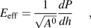
where A 0 is the contact area at the beginning of unloading. For an isotropic, elastic solid, the effective elastic modulus is related to specimen and indenter properties by

where E s and E d are Young’s moduli and ν s and ν d are Poisson’s ratios of specimen and indenter, respectively. β is a numerical factor first introduced by KingReference King23 that is often taken as  ≈ 1.13, but its value is debated.Reference Bolshakov, Pharr, Gerberich, Gao, Sundgren and Baker24–Reference Strader, Shim, Bei, Oliver and Pharr26 In previous studies,Reference Jakes, Frihart, Beecher, Moon and Stone27 we have found that β = 1.23 fits our data, and for consistency, use this value here. By varying the unloading rate, we anticipate being able to assess viscoelastic moduli in terms of
 over a wide range of time scale.
Interpretation of time-dependent load or unload data in the context of viscoelasticity is rendered difficult by the fact that analytical solutions for cone or pyramid indenters are not amenable to transform methods and are quite complicated.Reference Lee and Radok5–Reference Graham10 Approximations are therefore in order. Insight into one possible avenue is gained from Cheng and ChengReference Cheng and Cheng2 who studied two systems, a standard linear solid and the more general, linear viscoelastic solid with constant Poisson’s ratio. They showed that although dP/dh depends on history of loading, it becomes unique in the limit of high unloading rate:
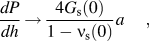
where a is the contact radius and G s(0) and ν s(0) are the shear relaxation modulus and Poisson’s ratio evaluated at zero time. This result is identical to the purely elastic case with β = 2/(π)2. For a glassy polymer, the quantity G s(0) is poorly defined because stiffness increases slowly across decades of time scale as t → 0. However, because Eq. (3) is taken as a limit, one may reasonably suppose that it remains valid if t = 0 is replaced with t = t ul (unloading time) provided t ul is much shorter than the hold time immediately prior to unloading. Such conditions would provide a way to measure G(t ul)/[1−ν(t ul)].
Previous researchers using Eqs. (1) and (2) as a basis for testing viscoelastic materials have identified experimental issues that we address in this paper. One issue is the accurate assessment of A 0. The most common method for determining A 0 is to use the contact depth,  , following the Oliver–Pharr approachReference Oliver and Pharr28 in which it is assumed that
 . However, numerous studies (e.g., Refs. Reference Cheng and Cheng29–Reference Tang and Ngan35) have shown that in viscoelastic solids,
 lacks uniqueness because unloading slope depends on unloading rate. We will overcome this difficulty by relying on images of residual indent impressions to measure A 0. Another issue is that
 assessed from a viscoelastic material depends on the load profile including times allowed for loading, hold, and unloading.Reference Fujisawa and Swain33, Reference Tang and Ngan35–Reference Tong, Sun, Chen and Zhang38 We will investigate the effects of hold and unloading times by systematically varying both. A final issue is the commonly observed phenomenon of a “nose,” or bulge, seen at the beginning of the unloading segment in load–depth traces.Reference Ngan, Wang, Tang and Sze34, Reference Chien-Kuo, Sanboh, Li-Piin and Nguyen39–Reference Briscoe, Fiori and Pelillo43 A nose appears when the depth continues to increase (rather than decrease) at the beginning of unloading before finally rebounding at lower loads. Systematic studyReference Ngan and Tang42 reveals that for a given hold time prior to unloading, the nose disappears if the unloading rate is made sufficiently rapid and that for a given unloading rate, the nose disappears if the hold time is made sufficiently long. When a nose is present, the usual method of measuring dP/dh from the unloading trace, which includes the assumption of a power law relation between load and depth during unloading,Reference Oliver and Pharr28 is no longer valid. Ngan and coworkersReference Ngan, Wang, Tang and Sze34, Reference Feng and Ngan41 developed a method for correcting dP/dh when a nose is present based on a Maxwell model (spring and dashpot in series), in which the nose is caused by the continued forward viscous deformation in the dashpot element during unloading. Their method and variations of it have been used to analyze a variety of materials including selenium,Reference Ngan, Wang, Tang and Sze34, Reference Tang and Ngan35 other metals,Reference Feng and Ngan41 structural polymers,Reference Fujisawa and Swain33, Reference Tang and Ngan35–Reference Fujisawa and Swain37, Reference Ngan and Tang42 and bone.Reference Tang, Ngan and Lu44 The nose effect is not unique to indentation. A nose also occurs in one-dimensional linear viscoelastic models if unloading occurs soon after loading (see example 2.8 in Ref. Reference Lakes1); however, inverse calculation based on linear viscoelasticity does not account for effects observed in the presence of viscoplastic indentation. We will show that for the materials studied, when a nose is present during unloading in nanoindentation, it is forward viscoplastic and not forward viscoelastic deformation that has occurred during the unloading.
The method proposed by Ngan and coworkersReference Ngan, Wang, Tang and Sze34, Reference Feng and Ngan41 to correct dP/dh when a nose is present relies on being able to measure the exact slope at the beginning of unloading. We have generally found this approach to be unsatisfactory. The slope obtained from a fit is highly sensitive to the form of the trial function used to generate the fit. This sensitivity is likely related to the fact that the slope at the beginning of unloading is ill-defined from a theoretical perspective. The immediate response of a viscoelastic solid to an abrupt discontinuity in the slope of the load-time curve (i.e., beginning of unloading) is dominated by the creep compliance evaluated at zero time, J(0). As discussed above, unlike the Maxwell model used by Ngan and coworkers, G(0) and therefore J(0) are ill-defined for glassy polymers. A much more robust method of fitting the data is to exclude the top portion the unloading curve to avoid the ambiguity there (such as advocated by Oliver and PharrReference Oliver and Pharr28) and rely, instead, on the unloading time itself as a basis for setting the time scale of the experiment. Although we disagree with Ngan and coworkers’ method for correcting dP/dh in the presence of a nose, we do agree with their assertion that forward creep can affect the unloading slope even if an obvious nose is not present. Therefore, below we develop an experimentally based criterion to remove from consideration indents with viscoplastic deformation detected during unloading.
In the present work, we characterize viscoelasticity across four decades of time scale. Unloading time is varied between 0.01 and 100 s. Hold time preceding unloading is varied between 0.05 and 100 s to help assess the viability of measuring G(t ul)/[1−ν(t ul)] when t ul << t hold. Indents which have detectable viscoplastic deformation during unloading are discarded. In the accompanying paper,Reference Jakes, Lakes and Stone45 we investigate the constant load creep hold segment of the nanoindentation experiments. During that segment, the areas of indents grow with time in a manner that unambiguously correlates with the viscoplastic properties of the polymers. Some of the viscoplasticity results are incorporated into this paper because they help us to interpret the viscoelasticity measurements. In addition, the nanoindentation viscoelastic moduli are compared with viscoelastic moduli measured using dynamic mechanical analysis (DMA) and broadband viscoelastic spectroscopy (BVS).
II. EXPERIMENTAL WORK
Materials studied include poly(methyl methacrylate) (PMMA), polycarbonate (PC), polystyrene (PS), and fused silica. The first three of these are all glassy polymers whose differences in viscoelastic and viscoplastic properties suffice to test the generality of methods developed in this work. Fused silica, comparatively low damping, helps to calibrate the measurements.
A. Nanoindentation specimens
The PMMA specimen was taken from a 3.33-mm-diameter extruded rod (density 1.15 g/cm3) obtained from Cope Plastics Inc. (Godfrey, IL). A 3-mm-thick cylinder was cut from the rod, and a surface was prepared for nanoindentation on the cross section perpendicular to the extrusion direction. For PC, specimens for nanoindentation and DMA were taken from a single, 1.59-mm-thick sheet of polycarbonate obtained from McMaster-Carr Supply Company (Aurora, OH). The extrusion direction of the sheet is unknown. The nanoindentation specimen was tested on a cross section perpendicular to the plane of the sheet. For PS, all specimens were made from a batch of polystyrene pellets (typical molecular weight of 280,000; glass transition temperature of 100 °C) obtained from Sigma-Aldrich Inc. (St. Louis, MO). The pellets were cylindrical shape with a length of about 3 mm and a diameter of about 2 mm. For nanoindentation, one of the pellets was first annealed at 110 °C for 2 h and then tested.
The surfaces for PMMA, PS, and PC specimens were all prepared for nanoindentation using a diamond knife fit in an ultramicrotome.
The fused silica was a Hysitron (Minneapolis, MN) calibration standard and was tested as-received.
B. Nanoindentation procedure
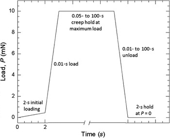
A Hysitron TI 900 TriboIndenter (Hysitron, Minneapolis, MN) equipped with Berkovich probe was used. The TriboIndenter was upgraded with a performech controller. The performech controller has faster electronics and increased data acquisition rates compared to the standard TI 900 TriboIndenter controller. The maximum data acquisition rate allowed by the TriboIndenter software is 38,000 points per second; however, the maximum number of data points the software will record for a given experiment is only approximately 209,000. Therefore, for each experiment the data acquisition rate was set as high as possible: either 38,000 points per second or the maximum rate possible to result in 209,000 total points. Figure 1 shows the basic load function used in this work. All indents were performed with open loop control to maximum loads of 10 mN. To generate the data for this paper, a load time of 0.01 s was used followed by hold and unload times that were systematically varied between 0.01 and 100 s. The 0.01 s time was chosen because it is the smallest time allowed by the TriboIndenter software. The longest time, 100 s, was chosen to minimize thermal drift effects. Thermal drift was measured before each experiment by holding the tip of the indenter probe in contact with a small force (2 μN) and monitoring the changes in displacement for times ranging from 10 to 300 s. The length of the thermal drift measurement segment was chosen to scale in proportion to the total time of the experiment. The final third of the thermal drift segment was fit to a straight line, and the displacement during the experiment was corrected using this drift rate. To minimize thermal drift, all experiments were run overnight. The average magnitude of thermal drift for all experiments was 0.04 nm/s, with 95% of the experiments less than 0.06 nm/s. The machine compliance for the indenter configuration used in this work was evaluated using data from a series of indents with different loads placed in the center of a fused silica standard and the SYS correlation.Reference Jakes, Frihart, Beecher, Moon and Stone27, Reference Stone, Yoder and Sproul46 Relative humidity in the nanoindenter enclosure was maintained between 33 and 35% using a glycerin–water bath. Temperature was not actively controlled but remained within one degree of 24 °C.
Basic load function used in this work. The 2-s hold at P = 0 ensured that load was accurately zeroed.

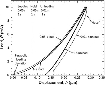
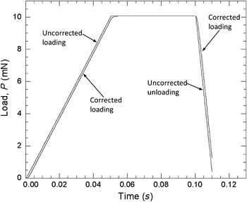
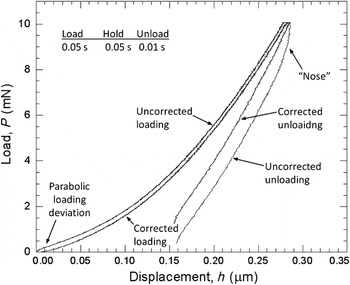
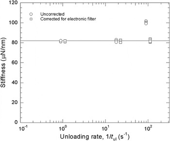
For experiments in which the load varies sufficiently rapidly, it is necessary to account for low-pass filter acting on the load transducer.Reference Asif, Wahl, Colton and Warren13 For the performech controller used in the present work, two of the three filters described in Ref. Reference Asif, Wahl, Colton and Warren13 are still present: a first-order filter acting on the load signal, and a first-order filter acting on the displacement signal; but the latter has a high cut-off frequency and does not appreciably affect the experiment even at the highest rates. Also, the component of mechanical filtering arising from the spring–mass-damping system is relatively minor because the indenter is in contact with the specimen. Most of the distortion of the load–depth signal comes from the load filter, but this distortion becomes significant only for load segments shorter than about 0.1 s. The effect is shown in load–depth traces from indents in fused silica in Fig. 2, where a deviation from the expected parabolic loading is present at the beginning of the load ramp lasting 0.05 s. In the unloading segment, which lasts 0.01 s, a “nose” is present. This “nose” is an instrumental effect and is unrelated to the “nose” caused by time-dependent deformation in the polymers as described in detail below. To correct the data, the first-order filter acting on the load can be modeled as a simple RC circuit with a 1-ms time constant, which allows the load–time curve like the fused silica load–time trace in Fig. 3 to be corrected using a simple convolution integral. The corrected load–depth trace for the 0.05-s load–0.05-s hold–0.01-s unload indent in Fig. 4 is similar to the 1-s load–1-s hold–1-s unload trace in Fig. 2. To check the validity of this approach, we show the measured stiffness of fused silica in Fig. 5 as a function of unloading rate (≡1/t ul, where t ul is unload time) for both uncorrected and filter-corrected data. Hysteresis in the fused silica is caused by viscoplasticity; otherwise fused silica is low-damping compared to the glassy polymers, so its elastic modulus should be relatively independent of unloading rate. For 1-s unloads, the filter has no effect; for 0.05-s unloads, the effect is barely detectable; and for the 0.01-s unload, the effect is large. However, the filter correction is able to remove this effect.
Indents placed in fused silica showing the effects of electronic filters on the high strain rate data. The effect of the filter is observed in the parabolic loading deviation in the 0.05-s load and in the “nose” of the 0.01-s unload.

Uncorrected and filter-corrected load–time traces for the 0.05-s load–0.05-s hold–0.01-s unload indent in fused silica in Fig. 2. The effect of the filter correction is to round off the corners and shift the loads to higher times.

Uncorrected and filter-corrected load–displacement traces for the 0.05-s load–0.05-s hold–0.01-s unload indent in fused silica in Fig. 2. In the corrected trace, parabolic loading deviation and nose are not present.

Effect of unloading rate (≡1/t ul) on the measured stiffness for 10-mN indents in fused silica with 0.01-, 0.05-, and 1-s unloads. The stiffness was measured in the usual way using a power law function to fit to 30–95% of the maximum load of the unloading trace. The data are offset slightly for clarity.

To calculate E s using Eqs. (1) and (2), values of E d and ν d for the diamond indenter are assumed to be 1137 GPa and 0.07, respectively. Values of ν s are assumed to be constants for each material and approximated as 0.37, 0.34, and 0.37 for PMMA,Reference Yee and Takemori47 PS,Reference Afifi48 and PC,Reference Fukuhara and Sampei49 respectively. The unloading portion of the load–depth trace is fit from 30 to 95% of the maximum load to the power law equation P = P′(h 0 − h)m in which P′, h 0, and m are used as fitting parameters.Reference Oliver and Pharr28dP/dh is then obtained from an extrapolation of the fitted curve up to the maximum load.
C. Atomic force microscopy
A Quesant (Agoura Hills, CA) atomic force microscope (AFM) incorporated in the Triboindenter was used to image all residual indents. Although most images were acquired 8–24 h after the indenter was removed, a select number of indents were repeatedly imaged at regular intervals on a log scale starting at 200 s and ending 4.9 days after unloading to determine whether the indent area changed with time. The AFM was operated in contact mode and calibrated using an Advanced Surface Microscopy Inc. (www.asmicro.com) calibration standard with a pitch of 292 ± 0.5 nm. Successive scans and calibration routines reveal the reproducibility of the AFM calibration to be ±1%. ImageJ (http://rsb.info.nih.gov/ij/) image analysis software was used to manually measure the contact areas, A 0, used in the analyses from 15-μm field-of-view images for the polymers.
D. Alternative assessment of viscoelastic properties
Capodagli and LakesReference Capodagli and Lakes50 previously reported BVS viscoelastic shear moduli measurements of PMMA taken from the same stock material studied here, so their results are available to compare with the present nanoindentation measurements. No such data existed for the PC and PS stock materials, so we used DMA to measure the viscoelastic Young’s moduli in these materials. A TA Instruments Q800 DMA (TA Instruments, New Castle, DE) fitted with a three-point bending fixture (50-mm span) generated storage Young’s modulus data of PS and PC from 10−2 to 10 Hz. For each of these two materials, three 60-mm-long beams with different cross sections were fabricated and tested. For PC, the beams were machined from the sheet from which nanoindentation specimens were taken. The three beams were all nominally 60-mm long and 1.59-mm thick. The three nominal beam widths were 3, 6, and 11 mm. For PS, stock bars were made by injection molding using a DSM Xplore (Geleen, The Netherlands) 15-ml microcompounder injection molder equipped with a bending bar mold (127 × 12.7 × 3.2 mm). Pellets from the same stock used for nanoindentation were first melted at 265 °C and then injection-molded by applying a pressure of 6 bar for 2 s followed by 7 bar for 6 s. From the injection-molded stock bars, three different size beams were machined. All beams were 60-mm long. Two beams were nominally 3-mm thick with one having an 11-mm width and the other 6 mm. The third beam had a nominal thickness of 1.5 mm and nominal width of 11 mm.
The cross-section dimensions of each beam were measured with an electronic caliper to the nearest 0.01 mm. The width and thickness were found to not vary more than ±0.01 mm along the length of the beam.
III. EXPERIMENTAL RESULTS
A. Assessment of contact area
Reliable nanoindentation measurements require an accurate assessment of contact area, A 0. As stated in the Introduction, A 0 calculated following the Oliver–Pharr approachReference Oliver and Pharr28 lacks uniqueness. We therefore rely on AFM images to measure A 0.
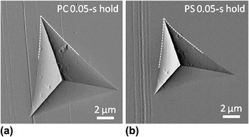
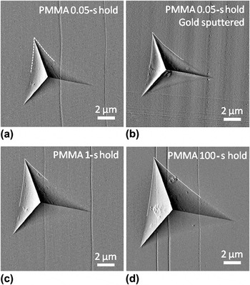
Contact areas are assessed from AFM images by using the contact edges to outline the indent. Contact edges can be identified by keying off of changes in surface texture in z-height images with slope shading. The method works well in PC and PS as well as PMMA with creep hold times greater than about 4 s [Figs. 6 and 7(d)], where the contact edges are sharp and easy to identify. For indents in PMMA with hold times less than about 4 s [Figs. 7(a) and 7(c)], the contact edges are more gradual and therefore more difficult to identify. To help with this problem, we sputtered the surface of a PMMA specimen with a thin layer of goldReference Strader, Shim, Bei, Oliver and Pharr26 and then placed a series of indents with different hold times into the sputtered surface. It was straightforward to identify the contact edges in the sputtered surface [Fig. 7(b)]; the knowledge gained helped us to identify the contact edges of indents in PMMA without sputtering [Figs. 7(a) and 7(c)].
AFM images of 10-mN indents in (a) PC and (b) PS. The dashed lines show the contact edges used for the assessment of contact area.

AFM images of 10-mN indents placed in PMMA. The dashed lines show the contact edges used for the assessment of contact area. To aid in identifying the contact edge, indents were also performed on PMMA sputtered with gold, as seen in b. The indent increases in size as the hold time at maximum load increases.

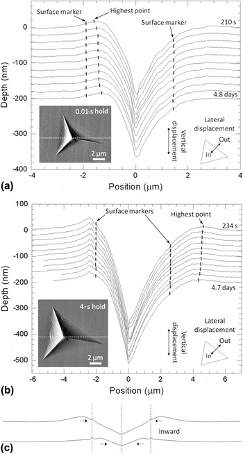
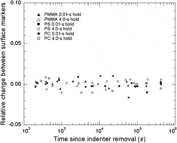
Some authors have claimed that areas of indents in polymers shrink over time following removal of the indenter.Reference Tweedie and Van Vliet51, Reference Low, Paglia and Shi52 To investigate how residual indents recover after unloading, we performed time-lapsed microscopy of indents placed in PMMA, PS, and PC. Representative depth profiles for indents in PMMA are shown in Fig. 8. At first glance, it might appear that the contact edges move laterally inward with time because the highest points in the depth profiles displace laterally inward. However, no lateral displacements are observed in the surface markers (scratches, asperities) of Fig. 8. Indents in PS and PC behave the same way. Data that quantify the lack of lateral movement of markers located near the edges of indents are presented in Fig. 9. To better than 0.5% uncertainty, the lateral separations between markers on opposite sides of the indents remained unchanged between 200 s and 4.9 days following removal of the indenter. By contrast, the depths of the same indents became 5–20% shallower over the times tested. We conclude that (i) depth recovery is at least one to two orders of magnitude larger than lateral recovery; (ii) lateral displacements of the highest points surrounding indents are caused not by lateral, inward displacements of material points on the surface, but instead by vertical displacements of the surface inside the indent [Fig. 8(c)]; and (iii) it is better to rely on changes in surface texture than on the highest points along ridges surrounding indents to specify the areas of indents because, unlike the highest points, the asperities that produce surface roughness do not move inward over time following removal of the indenter.
Depth profiles from time-lapse microscopy of 10-mN indent impressions in PMMA with (a) 0.01-s and (b) 4-s creep holds. Each profile is offset by 20 nm for clarity. The depth profiles were taken from AFM images of the indents collected at times from about 200 s to 4.8 days after the indenter was removed. Times were measured from the removal of the indenter to the time when the AFM scan reached the center of the indent. Surface markers were located visually at discontinuities in the profiles that arose from imperfections of the surface. The highest point markers were placed based on a third-order polynomial fit to the surface profile over a short segment. (c) Schematic showing the inward motion of the highest point, while surface markers maintain their separation.

Relative change in lateral separation between surface markers in PMMA, PS, and PC for both 0.01- and 4-s creep holds. There was no appreciable change in lateral separation detected in these experiments, which spanned times of about 200 s to 4.9 days after the removal of the indenter from the surface.

Researchers have reported using finite element models that lateral outward motions take place during unloading.Reference Chudoba and Jennett25, Reference Strader, Shim, Bei, Oliver and Pharr26 In the finite element models, surface nodes displace both laterally inward and vertically downward during loading and then laterally outward and vertically upward during unloading. Relative to its initial position before loading, a surface node at the contact edge immediately prior to unloading ends up displaced farther out laterally after unloading.Reference Chudoba and Jennett25 The lateral displacements of surface nodes observed in these finite element models arise from reversible, elastic deformations. Our experiments are unable to detect reversible changes in indent area that take place during unloading. However, as described in the next section, our experiments are able to detect irreversible increases in area during unloading.
Although we did not rely on Oliver–Pharr areas for our detailed calculations, we did evaluate them for comparison purposes. On average, the Oliver–Pharr areas for PMMA were about 7% larger than the AFM measurements, and the Oliver–Pharr areas for PS and PC were about 10% smaller than the AFM measurements.
B. Analysis of the unloading curves
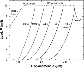
Figure 10 shows a series of load–depth traces from indents in PMMA, typical also of the traces for PC and PS. For these indents, the load times are 0.01 s and the hold times are all 0.25 s, but the unloading times, t ul, vary between 0.01 and 10 s. There is nothing unusual about the shapes of the load–depth traces for short unloading time, but as unloading time increases a visible nose begins to appear near the top of the unloading trace, similar to what has been reported elsewhere in the literature.Reference Ngan, Wang, Tang and Sze34, Reference Chien-Kuo, Sanboh, Li-Piin and Nguyen39–Reference Briscoe, Fiori and Pelillo43 The shape of this nose resembles the artifact caused by the electronic filters (Fig. 2), but the data of Fig. 10 have been corrected to remove that artifact. Also, the filter artifact only manifests for short t ul (<0.1 s), whereas the noses in the data of Fig. 10 only appear for longer t ul.
Load–depth traces of indents placed in PMMA. Each indent had a 0.01-s load and 0.25-s hold. The unload times ranged from 0.01 to 10 s. For clarity, unloading traces are offset horizontally in 0.2-μm increments.

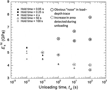
Preliminary viscoelastic moduli results for PMMA are shown in Fig. 11 for different combinations of hold and unloading times. Fitting unloading traces that exhibit noses to a power law obviously miscalculates dP/dh. For reasons described below, we will discard these data in the final analysis, but they are nevertheless included here. It is seen in Fig. 11 that for a given hold time, the elastic modulus first decreases then increases as unloading time increases from 0.01 to 100 s. The complete trend is most obvious in the data with 0.25-s hold time. A rise in elastic modulus for slower experiments is nonphysical for materials with positive damping.
Elastic modulus, E s, calculated for 10-mN indents in PMMA with various hold and unload times. The circled data indicate indents in which the contact area increased during unloading as will be seen in the apparent hardness in Fig. 13.

In every case where a nose or a rise in elastic modulus is seen from an indent with a long unloading time, the area of that indent is found from subsequent examination to have grown irreversibly during unloading. This effect is easy to detect because when indents are examined with AFM, those with short unloading times all have the same areas (depending only on loading and hold time), whereas those with long unloading times have comparatively larger areas. If the area of an indent grows during unloading, then the entire basis for measuring E s is violated, so the corresponding elastic modulus data must be discarded.
We prefer to work with hardness rather than area to demonstrate how to identify indents whose area grows during unloading. The Meyer hardness at the end of the constant load hold segment is defined in the usual manner as

where P 0 is the load and A 0 the area immediately prior to unloading. H 0 depends on loading time and hold time, but for obvious reasons, H 0 should not depend on unloading time. We therefore distinguish between H 0 and apparent hardness  =
 , where
 is the measured (or apparent) area assessed from an AFM image. In Figs. 12–14, the values of
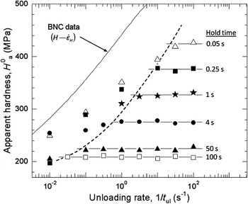
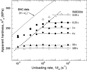
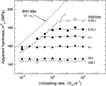
 for the indents with different hold times are plotted against unloading rate (≡1/t ul), for PMMA, PS, and PC. It is seen that for each hold time,
 is constant at sufficiently high unloading rate. These plateau values of
 are H 0 for each hold time.
 begins to drop once the unloading rate goes below a threshold value, which depends on hold time. Indents with
 lower than H 0 for a given hold time have areas that must have grown irreversibly during unloading. It is notable that sometimes
 indicates that the area has grown during unloading, even though no visible nose can be detected in the unloading trace. The indent with a 0.25-creep hold and 1-s unload in PMMA is an example of this effect. Although no nose is seen in the corresponding unloading trace (Fig. 10), the elastic modulus value from this indent is anomalously high (Fig. 11).
 therefore serves as a useful indicator to help eliminate from consideration elastic modulus data for which the indent areas have grown during unloading, even when the effect is not strong enough to produce a visible nose.
Apparent hardness,  , for PMMA indents. All indents have 0.01-s load times. The solid curve is a BNC hardness–indentation strain rate (H–
 ) curve from the accompanying paper.Reference Jakes, Lakes and Stone45 The dashed line shows the lower bound in 1/t ul for meaningful viscoelastic moduli data. It has the same shape as the BNC hardness–indentation strain rate (H–
 ) curve from the accompanying paper.Reference Jakes, Lakes and Stone45

Apparent hardness,  , for PS indents. See the caption for Fig. 12.

Apparent hardness,  , for PC indents. See the caption for Fig. 12.

Working with hardness also allows us to better understand the unloading nose (Fig. 10) and anomalous trends in viscoelastic moduli (Fig. 11). We see in Figs. 12–14 that H 0 depends on creep hold time, and in the accompanying paper, we analyze the change in hardness during the creep hold time to generate hardness–indentation strain rate (H– ) data using broadband nanoindentation creep experiments.Reference Jakes, Lakes and Stone45 In that paper, it is shown that the H–
 curves reflect the viscoplastic responses of the polymers to indentation. The solid curves in Figs. 12–14 are H–
 curves, and they have the same general shapes as the dashed curves, which show the threshold unloading rates in which
 begins to deviate from H 0 for each hold time. We therefore conclude that the root cause of the unloading nose and anomalous trend in elastic modulus is viscoplastic deformation during unloading. The separation between solid and dashed curves in Figs. 12–14 suggests that when the viscoplastic strain rate immediately prior to unloading approaches an appreciable fraction of unloading rate (8–20%, depending on material), the elastic modulus value becomes unreliable because, under these conditions, the unloading rate is sufficiently slow that the indent area has time to grow by viscoplasticity during unloading.
Last, we note the m values obtained from the unloading curves. Only those curves whose areas remained constant during unloading are included. The average fitted values of m are 1.7 for PMMA, 1.6 for PS, and 1.9 for PC. These are all high compared to the value of 1.3 for fused silica. The increased m in polymers has been reported by others.Reference VanLandingham, Villarrubia, Guthrie and Meyers53, Reference Briscoe and Sebastian54
C. Dependence of elastic modulus on hold time (hardness) and unloading time in PMMA, PS, and PC
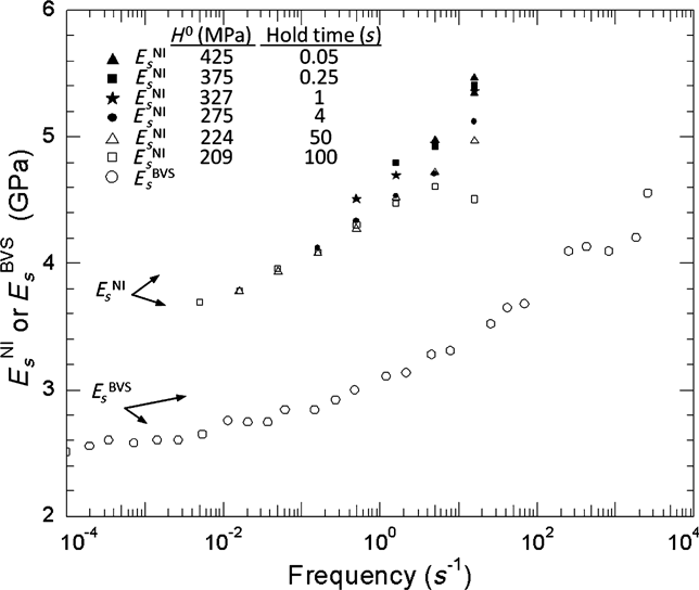
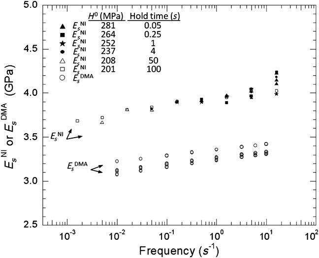
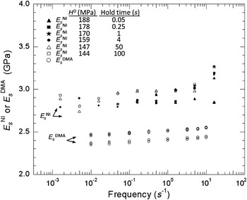
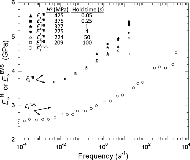
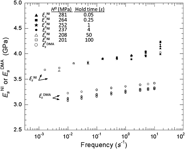
Viscoelastic moduli obtained from unloading traces are shown in Figs. 15–17. Only those indents for which the contact area does not change irreversibly during unloading are included. Viscoelastic properties measured using conventional BVS (PMMAReference Capodagli and Lakes50) and DMA (PS and PC) are compared with the nanoindentation data. The BVS experiments measure storage shear modulus and shear creep compliance, so to compare them with the nanoindentation data, we have converted them to E s assuming ν s = 0.37.Reference Yee and Takemori47 The values of viscoelastic moduli calculated using nanoindentation measurements are designated  , while those measured from DMA and calculated from BVS experiments are designated
 and
 , respectively.
 data for PMMA compared to
 data from Ref. Reference Capodagli and Lakes50.
 data for PS compared to
 data from DMA.
 data for PC compared to
 data from DMA.

Over the range tested with DMA and BVS, all the polymers have viscoelastic moduli that can be approximated as power law functions of frequency with power law exponents less than 0.1. This means that storage Young’s modulus, relaxation modulus, and 1/creep compliance should all agree to within better than 2%.Reference Lakes1 To compare the nanoindentation data with storage Young’s modulus, the usual transformation to frequency, ν = 1/2πt ul, is used.Reference Lakes1 It is seen in Figs. 15–17 that the nanoindentation viscoelastic moduli have the same trends with frequency as the viscoelastic moduli generated from DMA and BVS. However, the nanoindentation results are systematically higher than the DMA and BVS viscoelastic moduli. For PMMA,  is higher by about 37–50% than
 , depending on hardness (or hold time prior to unloading), but independent of frequency; in both PC and PS,
 is higher by about 18% than
 .
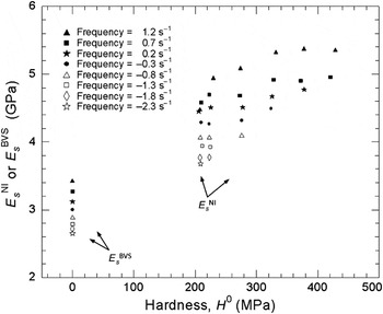
In PMMA, an increase in  can be observed with increasing hardness (Fig. 18). The effect is not as obvious in PC and PS; however, in these two materials the range of hardness is smaller than in PMMA, so the effect might be more difficult to detect. Also, the PC specimen appears not to have been entirely homogeneous, meaning that the properties varied by a small amount from place to place, which tends to obscure any trend that might be present in
 as a function of hardness.
Dependence of  on H 0 for indents in PMMA. Also included are
 values for the corresponding frequencies taken from Ref. Reference Capodagli and Lakes50. The
 data are plotted at H 0= 0.

IV. DISCUSSION
When the unloading time is sufficiently short compared to the hold time so that no irreversible changes in area take place during unloading, the elastic modulus data gained from nanoindentation experiments all follow similar trends (as functions of frequency) as the conventional data. This result lends credence to the idea that Eq. (3) is applicable except with t = 0 replaced by t = t ul. The question remains, however, why the nanoindentation viscoelastic moduli are systematically high. A number of factors could explain the increased elastic modulus, not the least of which is that nanoindentation measurements take place at finite strain, and nonlinearity might increase the elastic modulus,Reference Vanlandingham, Chang, Drzal, White and Chang21, Reference Anand and Ames55 pressure beneath the indenter might influence the measurement (Fig. 18 and Refs. Reference Veprek, Parks, Argon and Veprek56–Reference Wolf and Goken59), and viscoelastic properties can be sensitive to how they are measured. These topics are beyond the scope of the current paper but still need to be addressed to fully understand the meaning of the nanoindentation measurements.
One might reasonably ask whether our measurements depend on load. Measurements of hardness and modulus as functions of load are reported in the accompanying paper.Reference Jakes, Lakes and Stone45 From about 100 μN to 10 mN in PMMA and from 1.5 mN to 10 mN in PC and PS, we did not see an indentation size effect in either hardness or modulus. We do not, therefore, anticipate a change in viscoelastic properties across this range of loads although further verification should be made. At sufficiently low loads, a difference in viscoelastic response might become evident as a consequence of differences in near-surface polymer network topology.
V. CONCLUSIONS
Broadband nanoindentation techniques were developed to help measure viscoelastic properties from indents with unloading times between 0.01 and 100 s. We determine the following:
• The “noses” in unloading traces are associated with a hold time too short in comparison with unload time. They are associated with irreversible growth of the indent area during unloading and can be avoided by extending the hold time. They cannot be removed by inverse calculation of a linear viscoelastic model, owing to the viscoplasticity in the present experiments.
• Compared to viscoelastic moduli measured using BVS and DMA, the viscoelastic moduli measured from nanoindentation unloading traces possess the same trends with time or frequency but are 18–50% higher depending on material and creep hold time (hardness) prior to unloading. Experiments with areas that grow irreversibly during unloading must be discarded.
• The best way to measure time-dependent viscoelastic moduli from nanoindentation unloading slopes is to perform experiments with constant hold time and varying unloading time. A long hold time prior to unloading provides the widest dynamic range in measurement possible, subject to the bounds of electronic filters at short unloading times and viscoplasticity effects at long unloading times.
• We monitor the lateral motion of asperities (“surface markers”) in depth profiles from time-lapse microscopy of indent impressions. We find that the surface markers move neither inward nor outward after the indenter has been removed. In other words, the indents do not shrink or grow (to within 0.5% uncertainty in distance or 1% in area) after the indenter has been removed over the times tested (between 200 s and 4.9 days following removal of indenter).
• To best measure the areas of indents for calculation of hardness and modulus, one should rely on surface asperities rather than the surrounding ridges, or pileup, to define the edges of the indents. Area based on ridges changes with time following removal of the indenter, while area based on surface asperities remains constant.
ACKNOWLEDGMENTS
We thank Oden Warren, Syed Asif, Jason Oh, and Yuxin Feng at Hysitron Inc. for helping us to quantify the effects of the electronic filters in the nanoindentation measurements. Research was supported by CRADA 10-RD-111111129-027 between Hysitron Inc. and Forest Products Laboratory (J.E. Jakes) and by the National Science Foundation, Award CMMI-0824719 (D.S. Stone).