I. INTRODUCTION
The primary objective of the TanDEM-X (TDX) mission is the generation of a worldwide, consistent, timely, and high precision digital elevation model (DEM) aligned with the High Resolution Terrain Information-Level 3 (HRTI-3) specification as the basis for a wide range of scientific research, as well as for commercial DEM production [Reference Krieger, Moreira, Hounam, Werner, Riegger and Settelmeyer1]. This goal will be achieved by means of a second, TerraSAR-X (TSX) like satellite flying in close orbit configuration with TSX. Both satellites will then act as a large single-pass Synthetic Aperture Radar (SAR) interferometer with the opportunity for flexible baseline selection. This enables the acquisition of highly accurate cross-track and along track interferograms without the inherent accuracy limitations imposed by repeat-pass interferometry due to temporal decorrelation and atmospheric disturbances. Besides the primary goal of the mission, several secondary mission objectives based on along-track interferometry as well as new techniques with bistatic SAR have been defined which represent an important and innovative asset of the mission. TDX will be implemented in the framework of a public–private partnership between the German Aerospace Center Deutsches Zentrum für Luft- und Raumfahrt (DLR) and European Aeronautic Defence and Space Company (EADS) Astrium GmbH, as for TSX. The launch of TDX is planned for June 2010.
II. MISSION CONCEPT
The TDX mission is an extension of the TSX mission, co-flying a second satellite of nearly identical capability in a close formation. Among several options investigated, the Helix formation [Reference Krieger2] finally has been selected for operational DEM generation. The TSX satellite, as basis for TDX, is not only a high-performance SAR system with respect to SAR image and operational features, but it has already built in all necessary features required for the implementation of the TDX mission. Examples are additional X-band horn antennas for inter-satellite phase synchronization, the availability of a dual-frequency Global Positioning System (GPS) receiver for precise orbit determination, excellent Radio Frequency (RF) phase stability of the SAR instrument, and pulse repetition frequency (PRF) synchronization based on GPS as a common time reference. The second satellite (TDX) will be as much as possible a rebuild of TSX with only minor modifications like an additional cold gas propulsion system for formation fine tuning and an additional S-band receiver to enable the reception of status and GPS position information broadcasted by TSX. This guarantees a low development risk and it offers the possibility for a flexible share of operational functions among the two satellites. The TDX satellite will be designed for a nominal lifetime of five and half years and has a nominal overlap with TSX of three years. Note in this context that TSX holds consumables and resources for up to seven years of operation, allowing for a potential prolongation of the overlap and the TDX mission duration. The instruments on both satellites are advanced high-resolution X-band synthetic aperture radars based on active phased array technology, which can be operated in Spotlight, Stripmap, and ScanSAR mode with full polarization capability [Reference Stangl3]. The center frequency of the instruments is 9.65 GHz with a selectable SAR chirp bandwidth of up to 300 MHz. The active phased array antenna, which has an overall aperture size of 4.8 m × 0.7 m, is fixed mounted to the spacecraft body and incorporates 12 panels with 32 dual-pol slotted waveguide subarrays each. This enables agile beam pointing and flexible beam shaping.
A) Interferometric data acquisition
Interferometric data acquisition with the TDX satellite formation can be achieved in different operational modes: examples are bistatic, monostatic, and alternating bistatic operation. The three interferometric configurations may further be combined with different TSX and TDX SAR imaging modes like Stripmap, ScanSAR, Spotlight, and Sliding Spotlight. Operational DEM generation is planned to be performed using the bistatic InSAR Stripmap mode. This mode uses either TSX or TDX as a transmitter to illuminate a common radar footprint on the Earth's surface. The scattered signal is then recorded by both satellites simultaneously. This simultaneous data acquisition makes dual use of the available transmit power and is mandatory to avoid possible errors from temporal decorrelation and atmospheric disturbances.
B) Relative phase referencing
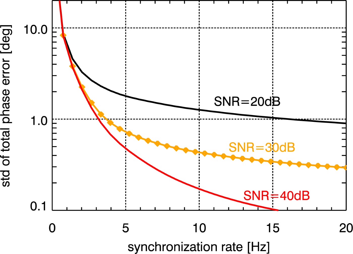
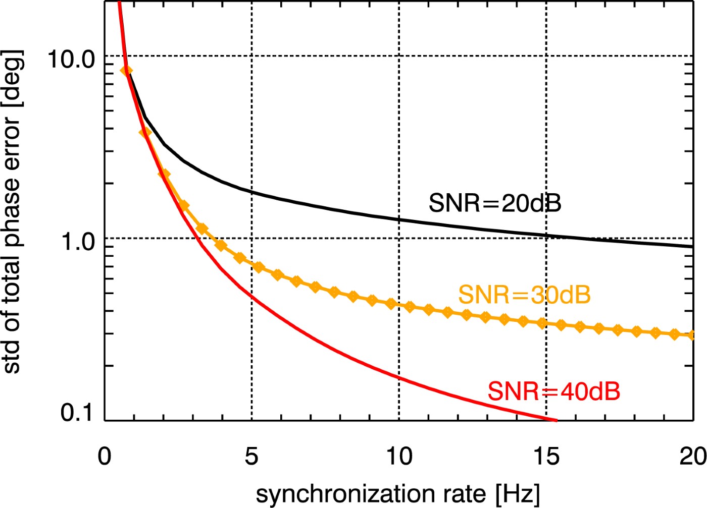
A peculiarity of the bistatic data acquisition is the use of independent oscillators for modulation and demodulation of the radar pulses. Any deviation between the two oscillators will hence cause a residual modulation of the recorded azimuth signal. The impact of oscillator phase noise in bistatic SAR has been analyzed in [Reference Krieger and Younis4] where it is shown that oscillator noise may cause significant errors in both the interferometric phase and SAR focusing. The stringent requirements for interferometric phase stability in the bistatic mode will hence require an appropriate relative phase referencing between the two SAR instruments or an operation in the alternating bistatic mode. For TDX, a dedicated inter-satellite X-band synchronization link will be established by a mutual exchange of radar pulses between the two satellites. For this, the nominal bistatic SAR data acquisition is shortly interrupted, and a radar pulse is redirected from the main SAR antenna to one of six dedicated synchronization horn antennas mounted on each spacecraft. The pulse is then recorded by the other satellite which in turn transmits a short synchronization pulse. By this, a bidirectional link between the two radar instruments will be established, which allows for mutual phase referencing without exact knowledge of the actual distance between the satellites. On ground, a correction signal can then be derived from the recorded synchronization pulses which compensates the oscillator-induced phase errors in the bistatic SAR signal. The performance of such a synchronization link has been investigated in [Reference Younis, Metzig and Krieger5]. Figure 1 shows the predicted standard deviation of the residual phase errors after synchronization as a function of the update frequency of the synchronization signals for different signal-to-noise ratios (SNR) of the bidirectional link. The actual SNR varies with the distance between the satellites as well as their relative attitude. For the typical DEM data acquisition mode with baselines below 1 km, the SNR will be in the order of 30–40 dB, and it becomes clear that a phase error below 1° can be achieved for synchronization frequencies of 5 Hz.
Standard deviation of the total synchronization link phase error as a function of the synchronization frequency. The standard deviation of the total phase error should be lower than 1° to meet the TDX requirements.
III. INTERFEROMETRIC PERFORMANCE
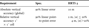
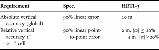
The main goal of the TDX mission is the generation of a global DEM consistent with the HRTI-3 specifications as listed in Table 1. The performance investigation in this paper concentrates on the impact of random errors expressed with the relative height accuracy, which is 2 m for terrain slopes |α| smaller than 20% and 4 m for terrain slopes greater than 20%.
HRTI-3 DEM specifications.
The key quantity in estimating the interferometric performance is the correlation coefficient γ, also called coherence, between two interferometric SAR images y 1 and y 2 [Reference Zebker and Villasenor6]:
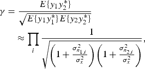
where E{·} is the expectation value operator and σx2 and σn1, 2i2 are the signal and noise source variances, respectively. It should be emphasized that this formula is valid for independent noise sources. Also the interferometric phase term has been neglected, since here only the magnitude of the coherence matters.
The total coherence γ is composed according to

where the right-hand side describes, the different error contributions due to the limited SNR (γSNR) (cf. the Appendix), quantization (γquant), ambiguities (γamb), limited coregistration accuracy (γcoreg), baseline decorrelation (γgeo), relative shift of Doppler spectra (γaz), volume decorrelation (γvol), and temporal decorrelation (γtemp). In non-vegetated areas the main driver of the coherence is the contribution due to the SNR.
The interferometer measures phase differences ϕ proportional to path length differences. This interferometric phase consists of the true interferometric phase ϕ0, related to the topography, and an interferometric phase error Δϕ introduced by the afore mentioned error sources. The distribution of the phase errors is described by Lee et al. [Reference Lee, Hoppel, Mango and Miller7] as a function of the number of looks N and the total coherence γ as
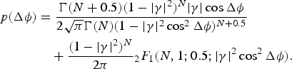
Here Γ denotes the gamma function and 2F 1 is the Gauss hypergeometric function. The relative 90% point-to-point height error Δϕ90% is defined via the integral over the difference probability density function (pdf) of two phase errors in a 1° × 1° cell, which corresponds in equatorial regions approximately to a 100 × 100 km2. Therefore, the joint pdf, which is given by the convolution of the single phase error pdf's

where * denotes convolution, has to be solved for Δϕ90%. Finally the 90% phase error transforms into the 90% height error Δh 90% proportional to the height of ambiguity h amb:
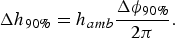
The height of ambiguity can be understood as phase to height scaling. A phase cycle of 2π corresponds to one height of ambiguity. This parameter depends only on the imaging geometry and the transmitted wavelength λ:

where r is the slant range, θi is the incidence angle and b ⊥ denotes the perpendicular baseline. For TDX, where the incidence angles vary between 30 and 48°, the perpendicular baselines are chosen between 200 and 600 m corresponding roughly to heights of ambiguities between 30 and 40 m.
In the next subsection the performance shall be estimated on a global scale by means of a so-called reference scenario.
A) Performance reference scenario
The reference scenario serves as basis for the judgment of the acquisition strategy. The current acquisition plan foresees at least two mappings of the global land mass. The generation of the final DEM requires therefore the combination of multiple interferograms, which is detailed in Section IV.C. The second acquisition is shifted with respect to the first one by half a swath width, which is approximately 15 km. For every acquisition and every swath a unique beam has been designed, such that the resulting height accuracy is well balanced.
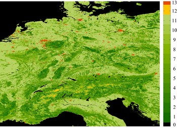
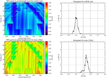
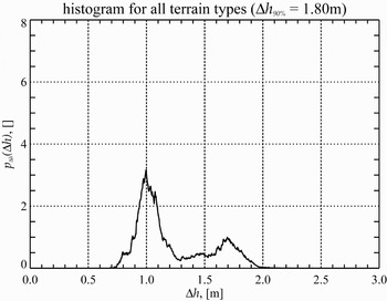
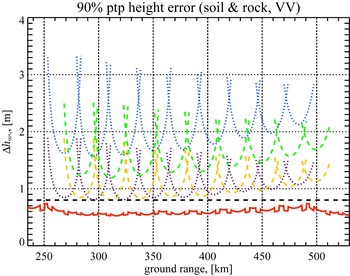
A fundamental input is the so-called global land cover classification map [Reference Hansen, DeFries, Townshend and Sohlberg8]. This map distinguishes the global landmass into 13 classes, like for example bare ground or mixed forest. Figure 2 shows the central part of Europe, consisting mainly of vegetated areas (1–12) whereas urban areas (13) and bare grounds (12) are less frequent. These classes can be associated with corresponding scattering classes, like trees or soil and rock. Additionally, vegetated areas are allocated a specific height in order to account for volumetric decorrelation effects. Figure 3 shows examples of the results for two scattering classes – soil and rock and trees. In the left column, the 90% point-to-point height error as function of the geographical latitude and ground range is depicted. On the right side, the corresponding histograms are plotted. As expected, the influence of volume decorrelation shifts the height errors towards higher values. These histograms form the basis for the global height error estimate. The histograms for the individual scattering classes are weighted with their global occurrence, as given in the global land cover classification map, and summed up. This results in a global height error distribution as presented in Fig. 4. The derived 90% height of 1.8 m is compliant to the HRTI-3 requirement.
Land cover classification map for central Europe.

Ninety percent height error after optimum combination (left column); histograms (right column).

Global height error distribution.

IV. PERFORMANCE IN HIGH DYNAMIC BACKSCATTER TERRAIN
In the afore presented performance prediction, a homogeneous backscatter distribution was assumed. This is an assumption that holds for example for large vegetated areas like rain forest or for deserts. But in densely populated areas, a high dynamic range in backscatter can be expected. Especially man made structures like urban areas will reflect back more energy than natural scenes. Of special importance are land city transitions, where low and high scatterers are in close neighborhood. Generally, a quantized signal is degraded by two error sources – granular noise and overload distortion or clipping errors. The effect considered here is called low scatterer suppression and is caused by inhomogeneous backscatter distributions. In the following the impact of quantization of signal returns from heterogeneous backscatter scenes on the height accuracy shall be analyzed.
A) The quantization effect
The quantizer used in the TDX and TSX satellite, respectively, is an 8-bit analog-to-digital converter (ADC) followed by a block adaptive quantizer (BAQ). The BAQ quantizes blocks of 128 samples of the input raw data stream u separately for the inphase- and quadrature-channel (u I and u Q). Based on the signal statistics, BAQ-specific parameters are calculated, which can vary from block to block. The compression levels are 8:2, 8:3, 8:4, 8:6, and 8:8, the last corresponds to BAQ bypass.
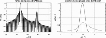
Figure 5 shows on the left side two different magnitude point targets in close vicinity after range processing as function of slant range r. In the raw data domain both targets will overlap significantly due to the large time bandwidth product of the transmitted waveform. For a given number of bits, the clipping voltage is calculated based upon the raw data signal power. This means that the quantization levels match best the strong signal, while the low magnitude signal is quantized very roughly. The effect of the quantization on the phase can be seen in the right plot of Fig. 5, where the interferometric phase error for a 2-bit quantization is evaluated at the mainlobe maxima of the strong signal (blue curve) and the low magnitude signal (orange curve). Consequently, regions with strong scatterers, which are quantized adequately will show low phase errors, while low backscatter regions are formidably more distorted. The amount of granular noise depends on the dynamic range of the backscatter.
Two point targets after focussing (left) and corresponding interferometric phase error distributions (right).

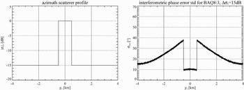
To demonstrate the quantization effect, an artificial scene with a rectangular scatterer profile in azimuth direction was simulated. The backscatter step height Δσ0 is 15 dB, which can be regarded as typical mean dynamic range in urban areas for X-band. Figure 6 shows the azimuth scatterer profile and the corresponding standard deviation of the interferometric phase error for a BAQ compression ratio of 8:3. The increase of the phase errors towards the region with high scatterer power between ±500 m can be clearly observed. The extension of the zone with increased errors is proportional to the azimuth beam width, which is in the order of 4 km for an incidence angle of 30°. In range direction the errors are spread proportional to the transmitted pulse length.
Azimuth scatterer profile (left) and standard deviation of the interferometric phase error (right).

B) Height error simulator
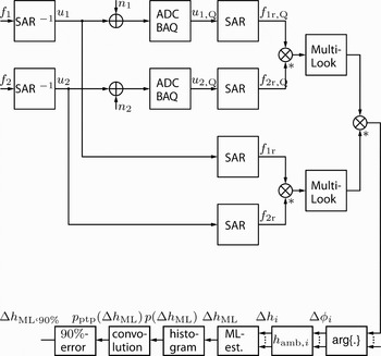
In order to estimate the impact of the quantization on the final interferogram, a simulation environment has been implemented. The simulation flow chart is illustrated in Fig. 7. Starting with an interferometric image pair f 1 and f 2 the corresponding SAR raw data u 1 and u 2 are generated by convolving the scene with the inverse focusing kernel. The raw data are superimposed by thermal receiver noise n 1 and n 2 and quantized by means of the ADC followed by the BAQ, resulting in the quantized raw data u 1,Q and u 2,Q. After focusing, the interferogram is formed from f 1r,Q and f 2r,Q. To reduce the speckle effect multilook processing is used, which is implemented as spatial low pass filter. The resulting interferometric phase is compared to the case where no thermal receiver noise and no quantization errors are present (lower path). The result is a phase error image Δϕi, where the index i, i ∈ [1, I], accounts for the ith realization. I does not necessarily coincide with the number of interferometric acquisitions. For instance, in overlap regions of adjacent swaths the number of interferogram pixels I to be fused at a single location is usually lager.
System model representing the interferometric chain with post processing.

The height error is calculated according to
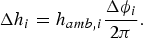
The height error is given as the difference between the measured height h and the true terrain height h 0

The step of combining multiple measurements is discussed in more detail in the next subsection. The 90% point-to-point height error Δh 90% is finally derived from the point-to-point height error distribution p ptp(Δh) = p(Δg) * p(Δh) (see equation (4)).
C) Interferogram fusion
A common method of combining measurements with unknown a priori density is by means of a maximum likelihood (ML) estimate. The task is to find the maximum of the conditioned density p(h|h 0) (likelihood function) of the measurement vector h = [h 1, h 2,…, h I]⊤

Assuming I independent height measurements h i the likelihood function is simply the product of the single measurement probability densities

The height error distribution can be derived from (3) with substitution as

The normalization is required to ensure
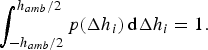
Taking the natural logarithm of the likelihood function and differentiating with respect to the true height h 0 yields a sum expression

Distribution (3) is based on the assumption that the backscatter coefficient can be modeled as circular complex Gaussian variate. Other popular backscatter models are for example the Weibull distribution or the K-distribution. Consequently, the final height estimate strongly depends on the underlying scatterer model. Moreover, pdf (3) requires the knowledge of the coherence γ, which also has to be estimated. And finally, the multilook processing, which is basically an averaging process, might allow to apply the central limit theorem for a sufficient large number of looks. Considering all these issues it might be justified to apply the Gaussian assumption directly to the height error Δh i. In this case, the ML estimator can be written in closed form, after substituting the Gaussian pdf's into (13) and solving for h 0, as

Since the estimator (14) is efficient the Cramer–Rao-Bound is given as
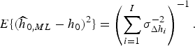
For equal height error variances σΔh i2 = σΔh2 the variance of the estimator according to (15) would be Δh2/I. The advantage of estimator (14) is that it only depends on the height error variances, which can be estimated from the interferograms. It should be mentioned that an initial digital elevation model is required [Reference Eineder and Adam9] in order to find the absolute terrain height h 0, since every height measurement is ambiguous with a period of h amb,i.
For the purpose of simulation the true terrain height h 0 is set to zero.
D) Simulation results
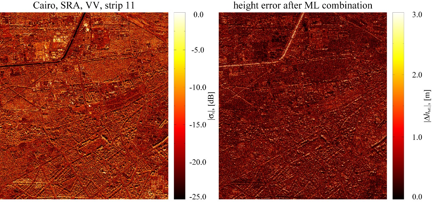
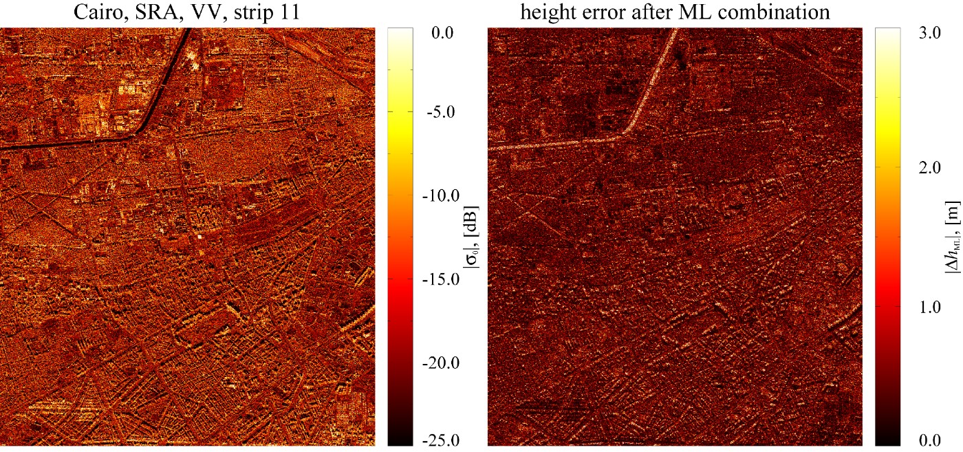
The following simulations are based on TSX measurement data utilizing the flowchart in Fig. 7. The first simulation is performed over urban area, as depicted in the left image of Fig. 8, which is a part of the Cairo city center. This scene offers a high dynamic range in backscatter power with a dynamic range in the order of 15 – 20 dB. On the right-hand side of Fig. 8 the corresponding height error after ML combination is presented. Here a mean SNR of 10 dB for both interferometric acquisitions is assumed and a BAQ of 8:3 was used. The heights of ambiguities are 30 and 40 m, respectively. Both images are multilook processed with 16 looks. As expected, the strong scatterers are less distorted than the low scatterer regions, like the roads. The histogram in the upper left image of Fig. 9 shows the distribution of the height errors for 16 looks, BAQ8:3 and a height of ambiguity of 30 m for a single acquisition. The 90% height error of 2.13 m does not meet the requirement. With a second acquisition, again with a height of ambiguity of 30 m, the height error decreases with a factor of  to 1.51 m, as predicted by formula (15). This example shows that at least two interferometric acquisitions are required in order to fulfill the HRTI-3 standards. The lower left and the lower right pictures of Fig. 9 demonstrate the improvement in height accuracy by increasing the number of BAQ bits from 3 to 4. In this case, the improvement is 0.23 m. If the data rate does not put a constraint a finer quantization allows to reduce height errors, especially in difficult terrain.
SAR intensity image of Cairo (left) and corresponding interferometric height error for BAQ8:3 (right).
Histogram for the point-to-point height error for a single acquisition over Cairo (upper left) and after optimum combination of two interferometric acquisitions (upper right); histogram for BAQ8:3 with nominal heights of ambiguities of 30 and 40 m (lower left) and for BAQ8:4 (lower right).

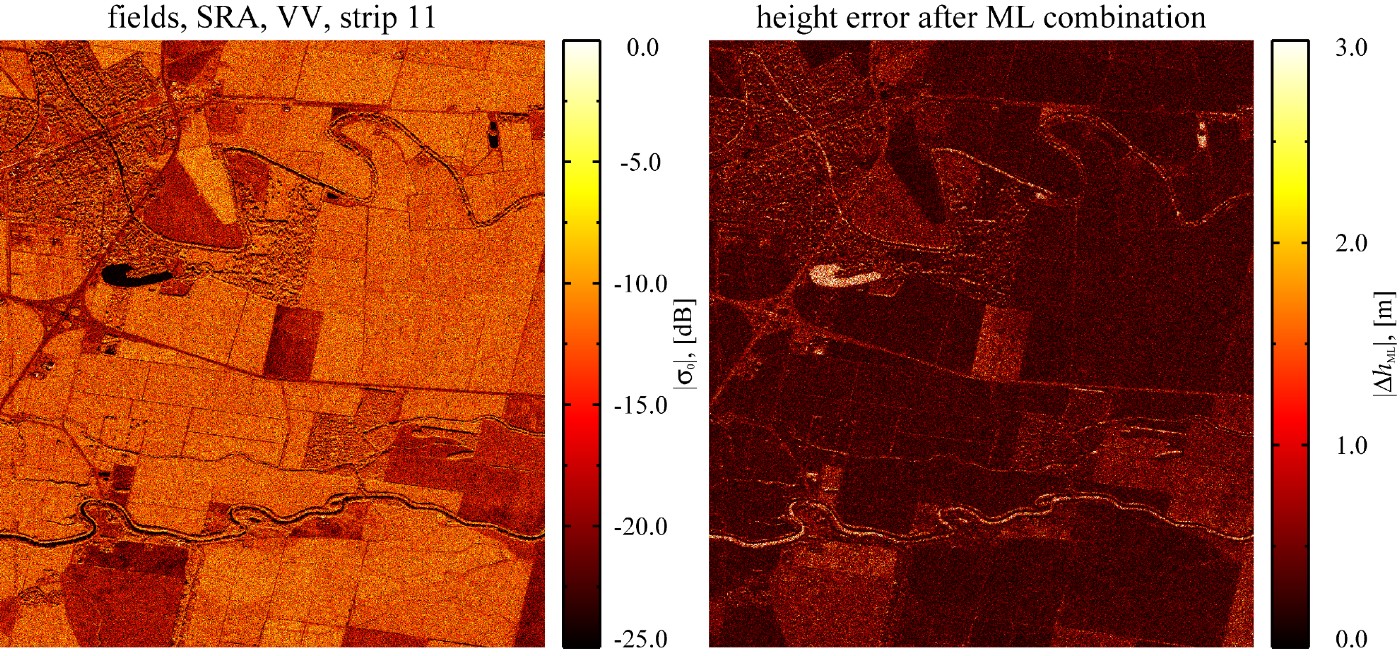
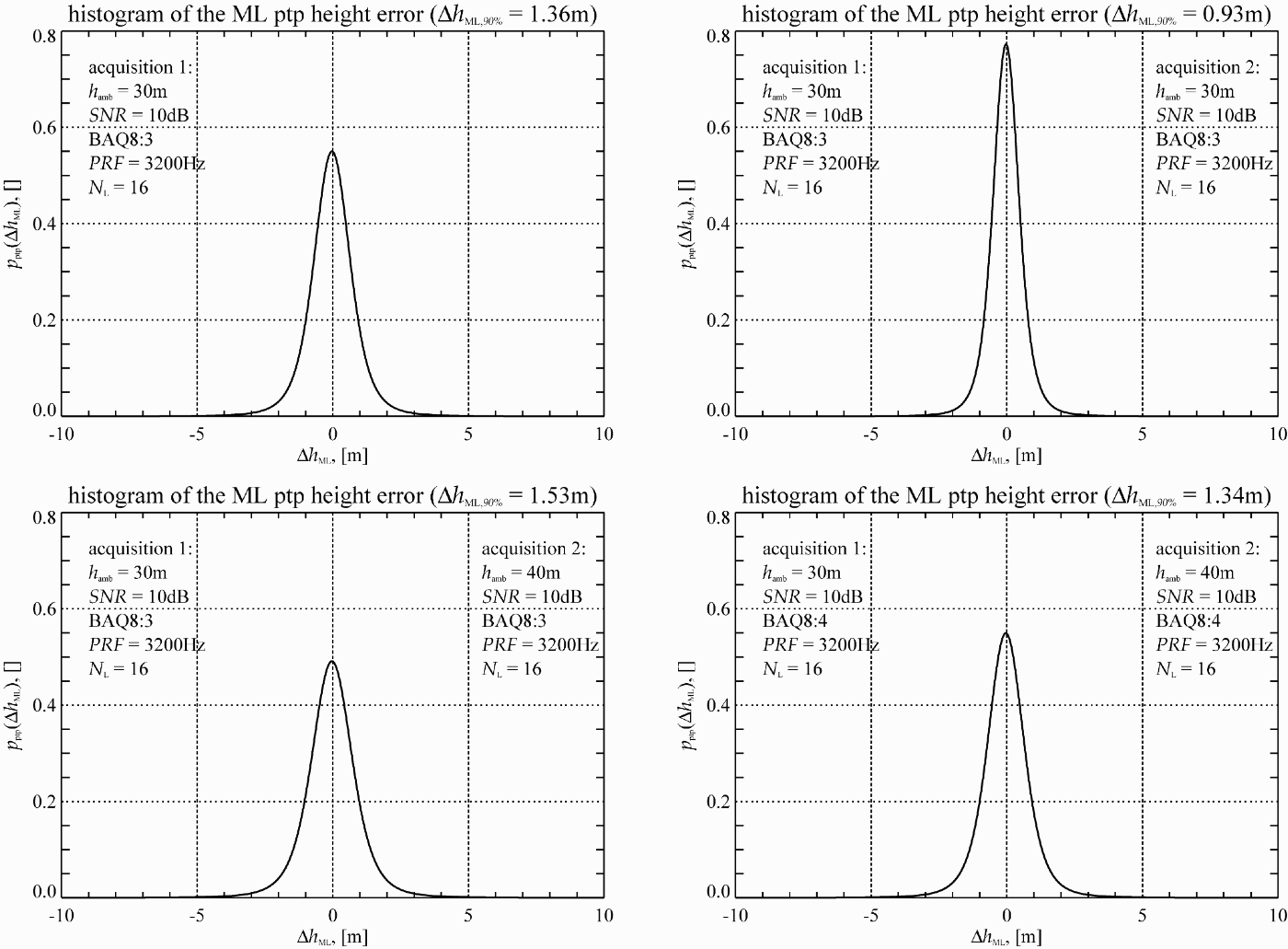
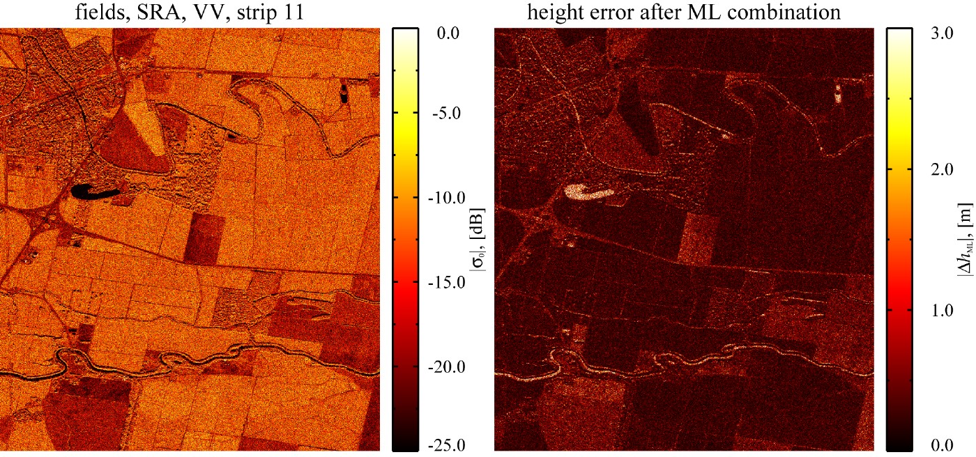
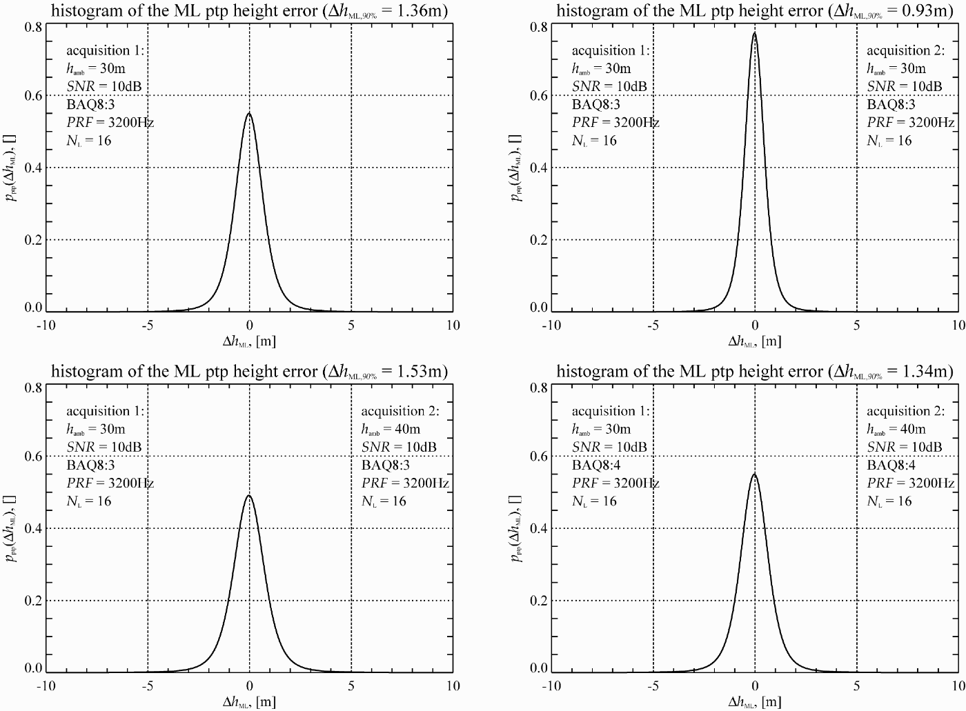
Another example is shown in Fig. 10 on the left. Here the SAR intensity image of an agricultural area is presented. These regions reflect microwave energy quite differently, even in X-band. The height error map on the right shows large height errors in low backscatter regions, using the same simulation parameters as before. The histograms in Fig. 11 show the analog simulation results to Fig. 9. Here the height errors are lower compared to the height errors over Cairo.
SAR intensity image of agricultural sizes (left) and corresponding interferometric height error for BAQ8:3 (right).
Histogram for the point-to-point height error for a single acquisition over fields (upper left) and after optimum combination of two interferometric acquisitions (upper right); Histogram for BAQ8:3 with nominal heights of ambiguities of 30 and 40 m (lower left) and for BAQ8:4 (lower right).
V. NEW IMAGING TECHNIQUES
The TDX mission will provide the remote sensing scientific community with a unique data set to exploit the capability of new bistatic radar techniques and to apply these innovative techniques for enhanced geo- and biophysical parameter retrieval. TDX is predestined for along-track interferometry (ATI), which compares the phase of two complex SAR images acquired in identical geometries but separated by a short time interval. Digital beamforming combines the RF signals from a set of small non-directional antennas to simulate a large directional antenna. Due to the split antennas and dual receiver channels of TSX and TDX, four phase centers can be obtained in a tandem mode.
A) Very large baseline cross-track interferometry
Very large baseline interferometry takes advantage of the high RF bandwidth of the TSX and TDX satellites, which allows for coherent data acquisitions with baselines of up to 5 km and more. Note that less than 5% of the maximum possible (critical) baseline length is used during nominal DEM data acquisition. Large baseline interferograms can hence significantly improve the height accuracy, but the associated low height of ambiguity requires a combination of multiple interferograms with different baseline lengths to resolve phase ambiguities. By this, it becomes possible to derive DEMs with HRTI-4 like accuracy on a local or even regional scale. Figure 12 shows a height accuracy example using the combination of four interferometric acquisitions with two additional orthogonal baselines in the order of 1.4 km. From this example, it becomes clear that in vegetation free and temporal stable areas DEMs with accuracies fulfilling the HRTI-4 requirements can be generated. Further opportunities arise from a comparison of multiple large baseline TDX interferograms acquired during different passes of the satellite formation. This provides a very sensitive measure for vertical scene and structure changes. TDX enables hence the entry into a new era of interferometric (and tomographic) processing techniques as it was ERS-1/2 for the development of classical repeat-pass SAR interferometry.
Height accuracy prediction for four interferometric acquisitions with heights of ambiguities of 30 and 40 m and two times 9 m. The posting is 6 m.

VI. CONCLUSION
TDX is a highly innovative bistatic single-pass SAR interferometer which allows for the acquisition of unique remote sensing data products. The achievable height accuracy for global DEM generation with TDX is mainly limited by the height of ambiguity that can finally be processed during phase unwrapping. The standard HRTI-3 DEM is a reasonable compromise between performance, processing, and data acquisition effort. A mission scenario has been developed which enables the acquisition of a global HRTI-3 DEM within less than three years. This concept includes several data takes with different baselines, different incident angles, and data takes from ascending and descending orbits to deal with difficult terrain like mountains, valleys, tall vegetation, etc. The TDX mission concept allocates also sufficient acquisition time and satellite resources to secondary mission goals like along-track interferometry or the demonstration of new bistatic radar techniques.
ACKNOWLEDGEMENT
The TanDEM-X project is partly funded by the German Federal Ministry of Economics and Technology (Förderkennzeichen 50 EE 0601).
APPENDIX A
Let the SAR raw signal, received by the mth channel of an array antenna be represented by its power spectral density as function of frequency f and Doppler frequency f D
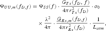
where ΨSS(f) is the power spectrum of the transmitted waveform, σ0 denotes the radar cross section per resolution cell  and L atm accounts for atmospheric losses. G Tx is the transmit gain pattern and
 is the mth complex element gain pattern with respect to a reference point, which is typically the geometrical center of an array antenna aperture

where  is the element space factor and the factor of two in the exponential accounts for power. k = 2π/λ is the wavenumber and r m is the distance of the mth element to the reference point. The signal is combined coherently in the power combiner network (PCN). In the following, the frequency variables are skipped for notational simplicity. Then the combined SAR raw data power spectrum ΨUU can be written as
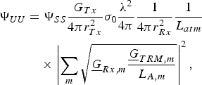
with the complex TR module amplification  and the antenna element losses L A,m. Note that usually the antenna losses are already contained in the gain defined at the ports of an antenna. The final SAR image power spectrum ΨYY is obtained by processing. It should be mentioned that the above expression is part of the SAR imaging equation. The exact solution is the inversion of an integral equation. A good approximation, especially for the space borne case, is to express the SAR focusing operation by a multiplication of the SAR raw data power spectrum with a filter power spectrum ΨHH

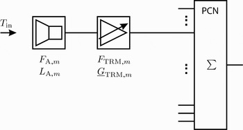
For the thermal receiver noise the noise figure concept can be exploited. A simplified block diagram of the receive path is depicted in Fig. 13. Generally, the output noise power spectral density for a series connection of N 2p, N 2p ≥ 2, linear two ports can be written as
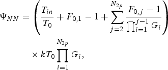
assuming white Gaussian noise. F 0 is the noise figure given at a reference temperature T 0, G is the corresponding gain and T in is the input noise temperature which corresponds in X-band approximately to the earth surface temperature. Substituting





into equation (A.3) yields
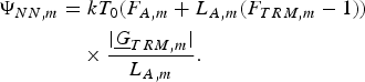
Block diagram of the receive chain.

If the assumption, that the antenna noise figure F A,m is equal to its loss L A,m [Reference Lee10] is valid, then the above equation reduces to

The noise power is combined incoherently in the PCN and filtered according to
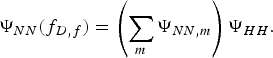
Then the SNR of the SAR raw data can be written
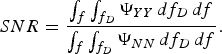
The frequency domain representation of equation (A.14) reveals a problem, since here only the average signal power can be calculated. This means, that the compression gain in the focused SAR image SNR is lost. To circumvent this problem the SNR can be estimated by combining the total available signal- and noise-power according to
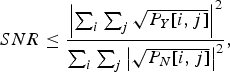
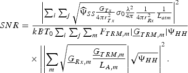
where i = 1, … , N r and j = 1, … , N a account for the samples to be combined. N r = τpB is the number of samples in range, with τp the pulse duration and B the signal bandwidth. N a = τintPRF is the number of samples in azimuth, with τint the integration time in azimuth:
Here the normalized signal power spectrum is defined as
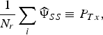
where P Tx is the transmitted peak power. Assuming equal antenna losses L A for every channel and with the definition of the gain for array antennas
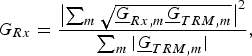
and the equivalent noise figure
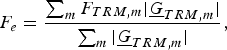
the expression for the SNR can be simplified yielding
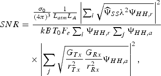
with the filter power spectrum separated in range and azimuth ΨHH[i, j] = ΨHH,r [i] · ΨHH,a[j]. This derivation can be easily expanded to lossy power combiner networks.
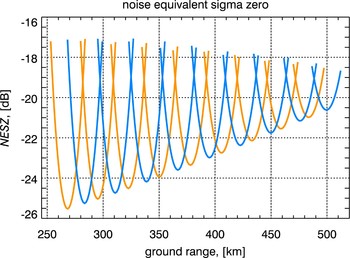
A performance measure for a SAR instrument is the noise equivalent sigma zero, which is defined  . Figure 14 shows the NESZ for the TDX spacecrafts for the two interferometric acquisitions.
Noise equivalent sigma zero for the TanDEM-X satellites.

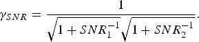
Finally, for an interferometer with unequal SNRs the resulting coherence would be
 Sigurd Huber received the Dipl.-Ing. (M.S.) degree in electrical and communication engineering from the Technical University of Munich, Germany, in 2005. Since 2005, he works as a scientist at the Microwaves and Radar Institute (HR) of the German Aerospace Center (DLR), Oberpfaffenhofen, Germany. He is involved in the conception of future SAR systems, utilizing advanced hardware architectures, as well as digital beam forming techniques. His research interests include digital signal processing, electromagnetic field theory, and inverse problems.
 Marwan Younis (S'1995, M'2005, SM'2008) was born in Las Cruces, USA, in 1970. He received his B.Sc. in electrical engineering from the University of Baghdad, Iraq in 1992 and the Dipl.-Ing. (M.Sc.) and Dr.-Ing. (Ph.D.) degree in electrical engineering from the Universität Karlsruhe (TH), Germany, in 1997 and 2004, respectively. From 1998 to 2004, he was a research scientist with the Institut für Höchstfrequenztechnik und Elektronik, Universität Karlsruhe (TH). Since 2005 he has been with the Microwaves and Radar Institute of the German Aerospace Center (DLR), Oberpfaffenhofen, Germany. He is the author and co-author of over 40 conference papers and more than 15 reviewed publications. His research fields include synthetic aperture radar (SAR) systems, digital beamforming for radar, synchronization of bistatic SAR, forward looking radar, and antennas. Dr. Younis is an active member of the IEEE and the German Association for Location and Navigation (DGON). He is working group leader within the IEEE instruments and future technologies technical committee. He is a lecturer with the Universität Karlsruhe (TH). He received the Hermann-Billing award for his Ph.D. thesis in 2005.
 Gerhard Krieger received the Dipl.-Ing. (M.S.) and Dr.-Ing. (Ph.D.) degrees (with honors) in electrical and communication engineering from the Technical University of Munich, Germany, in 1992 and 1999, respectively. From 1992 to 1999, he was with the Ludwig-Maximilians University, Munich, where he conducted multidisciplinary research on neuronal modeling and nonlinear information processing in biological and technical vision systems. In 1999, he joined the Microwaves and Radar Institute (HR) of the German Aerospace Center (DLR), Oberpfaffenhofen, Germany, where he developed signal and image processing algorithms for a novel forward looking radar system employing digital beamforming on receive. From 2001 to 2007, he led the New SAR Missions Group which pioneered the development of advanced bistatic and multistatic radar systems as exemplified by the forthcoming TanDEM-X mission as well as innovative multi-channel SAR techniques and algorithms for high-resolution wide-swath SAR imaging. Since 2008, he has been Head of the new Radar Concepts Department of the Microwaves and Radar Institute, DLR, Oberpfaffenhofen, Germany. Dr. Krieger received several national and international awards, including the IEEE Transactions Prize Paper Award of the Geoscience and Remote Sensing Society and the Otto Lilienthal Sabbatical of the German Aerospace Center, DLR. He is author of 30 peer reviewed journal papers, 4 invited book chapters, more than 100 conference papers, and 4 patents. His current research interests focus on the development of multi-channel radar techniques and algorithms for innovative MIMO SAR systems, the demonstration of novel interferometric and tomographic Earth observation applications, and the conceptual design of advanced bi- and multi-static radar missions.