1 Introduction
The study on the flow around an obstacle moving vertically in a stratified fluid would be traced back to a paper by Mowbray & Rarity (Reference Mowbray and Rarity1967), which showed how the far-field internal wave patterns generated by a sphere vary with the Froude number. After that work however, there have been only a small number of studies on this problem for nearly thirty years, with almost no observations on the near-wake structure. One of the exceptions would be the shadowgraph experiments by Ochoa & Van Woert (Reference Ochoa and Van Woert1977) which observed the vertical ‘filament’ at the rear of the sphere.
The problem began to be investigated more intensively at the end of the 1990s. The descent of a small particle in a two-layer fluid with a sharp density interface was investigated by Srdić-Mitrović, Mohamed & Fernando (Reference Srdić-Mitrović, Mohamed and Fernando1999), and the flow around a sphere in a linearly stratified fluid at moderate Reynolds numbers was investigated numerically by Torres et al. (Reference Torres, Hanazaki, Castillo and Van Woert2000). Significant increase in the drag coefficient
 $C_{D}$
was observed in these studies, up to nearly twenty times of that in the homogeneous fluid. In Srdić-Mitrović et al. (Reference Srdić-Mitrović, Mohamed and Fernando1999) the increase of drag was mainly explained by the buoyancy force on the caudal fluid dragged from the upper layer into the interfacial stratified fluid. On the other hand, Torres et al. (Reference Torres, Hanazaki, Castillo and Van Woert2000) found a strong vertical ‘jet’ at moderate Reynolds numbers which would correspond to the filament observed in Ochoa & Van Woert (Reference Ochoa and Van Woert1977). The jet significantly reduces the pressure at the rear of the sphere, and it would explain the huge increase of drag coefficient in stratified fluids. In an experiment for moderate Reynolds numbers, Abaid et al. (Reference Abaid, Adalsteinsson, Agyapong and McLaughlin2004) observed an oscillatory motion of a freely descending sphere and considered a mathematical model to describe the phenomenon.
At low Reynolds numbers, the problem is closely related to the vertical settling of the planktons and the ‘marine snow’ of small organic particles, both of which play a key role in the oceanic carbon cycle (e.g. Shanks & Trent Reference Shanks and Trent1980). Yick et al. (Reference Yick, Torres, Peacock and Stocker2009) performed experiments and numerical simulations at low Reynolds numbers (
 $Re\lesssim 1$
), and reported a drag coefficient several times larger than that in the homogeneous fluid. They found that the magnification of the drag coefficient
 $C_{D}$
by stratification is
 $Re^{1/2}/Fr$
. Multiplying the Stokes drag in homogeneous fluid (
 $\propto 1/Re$
), the drag coefficient in stratified fluids becomes
 $C_{D}\propto 1/(Re^{1/2}Fr)$
. This result is consistent with Torres et al. (Reference Torres, Hanazaki, Castillo and Van Woert2000), which showed that the drag increases like
 $\propto 1/Fr$
at fixed moderate Reynolds numbers (cf. D’Asaro Reference D’Asaro2003). Camassa et al. (Reference Camassa, Falcon, Lin, McLaughlin and Mykins2010) investigated how the descending velocity of a sphere decreases when the sphere deforms a sharp density interface of a two-layer fluid. They used the Stokes approximation at very low Reynolds numbers (
 $O(10^{-5})<Re<O(10^{-2})$
) assuming no density diffusion and no internal waves, and found that the predicted sphere velocity agrees with their experiments.
While all the other simulations have been performed for the steady movement of a sphere, the unsteady settlement of the sphere was simulated by Doostmohammadi, Dabiri & Ardekani (Reference Doostmohammadi, Dabiri and Ardekani2014), which gave good comparison of the transient sphere velocity with the previous experiments at low Reynolds numbers (
 $Re\lesssim 1$
).
At moderate Reynolds numbers, the problem would be applied to larger obstacles, e.g. to the control of the vertical motion of a Lagrangian float such as an Argo float, which is released into the deep ocean to observe the ocean current, temperature and salinity which constitute the fundamental data set of the ocean circulation. The increase of drag in proportion to
 $1/Fr$
at low speed (Torres et al.
Reference Torres, Hanazaki, Castillo and Van Woert2000) has been actually used for the development of a Lagrangian float (D’Asaro Reference D’Asaro2003).
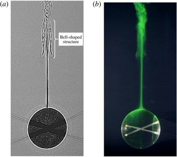
Visualisation of the flows around a sphere descending in a strongly stratified fluid at moderate Reynolds numbers (reproduced from figures 5a and 7 of Hanazaki, Kashimoto & Okamura Reference Hanazaki, Kashimoto and Okamura2009a
). (a) Shadowgraph image at
 $(Fr,Re)=(0.32,199)$
; (b) dye visualisation at
 $(Fr,Re)=(0.30,245)$
. The vertical jet and the bell-shaped structure observed at
 $z^{\ast }/(2a^{\ast })=1.5\sim 2$
(
 $z^{\ast }=0$
is the height of the sphere centre) are the unique structures of the flow.

In experiments for a sphere moving at constant speed, Hanazaki et al. (Reference Hanazaki, Kashimoto and Okamura2009a
) found at moderate Reynolds numbers that there are seven types of wake/jet in the parameter range of
 $0.2\lesssim Fr\lesssim 70$
and
 $30\lesssim Re\lesssim 4000$
. They confirmed the existence of ‘jets’ predicted by the previous numerical simulation (Torres et al.
Reference Torres, Hanazaki, Castillo and Van Woert2000) and found a peculiar ‘bell-shaped’ structure which is generated by the downward flow pertinent to the internal waves (figure 1).
In a numerical simulation, Hanazaki, Konishi & Okamura (Reference Hanazaki, Konishi and Okamura2009b
) investigated the effects of the Schmidt number, and found that the jet becomes broader and weaker for smaller Schmidt numbers, suggesting a strong relationship between the density diffusion and the rear jet. More recently, the initial process of jet formation was investigated by Hanazaki, Nakamura & Yoshikawa (Reference Hanazaki, Nakamura and Yoshikawa2015), and they confirmed that the generation of a jet actually has its origin in the density diffusion. Initially, the descending obstacle simply pulls down the originally horizontal isopycnic surface, deforming its shape. However, as time proceeds, density diffusion becomes effective, especially in the density boundary layer around the sphere, and the fluid of non-conserved density is detached from the isopycnic surface and moves upward to return approximately to its original height, generating a buoyant jet. They investigated at the same time how the radius of the jet and the thickness of the velocity boundary layer around the sphere depend on the Froude number and the Reynolds number, and found that they are approximately given by the primitive length scale of the stratified fluid, i.e.
 $l_{\unicode[STIX]{x1D708}}^{\ast }=\sqrt{\unicode[STIX]{x1D708}^{\ast }/N^{\ast }}$
(Gibson Reference Gibson and Nihoul1980) (
 $\unicode[STIX]{x1D708}^{\ast }$
: kinematic viscosity of the fluid,
 $N^{\ast }$
: Brunt–Väisälä frequency), or by
 $l_{\unicode[STIX]{x1D708}}^{\ast }/2a^{\ast }=(Fr/2Re)^{1/2}$
(
 $a^{\ast }$
: radius of the sphere) in its non-dimensional form.
Besides its significance in application, measurement of the fluid velocity at moderate Reynolds numbers would be important since the investigations at low Reynolds numbers have been performed using inevitably very small particles, making it difficult to observe the details of the flow, especially the fluid velocity around the obstacle and in the wake/jet region. Indeed, almost all the recent experiments observe only the descending speed of a freely falling sphere/particle, and do not measure the fluid velocity around it. An exception is the paper by Hanazaki et al. (Reference Hanazaki, Kashimoto and Okamura2009a ) which reported the fluid velocity observed by particle image velocimetry (PIV), but it was only for two sets of Froude and Reynolds numbers.
Therefore, more systematic velocity measurement is necessary to verify the parameter dependence of the flow as predicted by the numerical simulations. In this study, we measure the velocity distributions around a sphere descending at constant speed, and investigate the Froude number and the Reynolds number dependence of the velocity distributions to examine the recent predictions by numerical simulations of the buoyant jet and the boundary layer of the sphere (Hanazaki et al. Reference Hanazaki, Nakamura and Yoshikawa2015).
We should note here that it is usually difficult in experiments to vary only one of the two parameters
 $Fr$
and
 $Re$
, while it is easy in numerical simulations. The experiments on one day are usually performed using the same stratified fluid (
 $N^{\ast }=\text{const.}$
) since it takes a long time to generate a stratified fluid. In addition, a sphere of constant and large radius
 $a^{\ast }(=2~\text{cm})$
is used throughout the present experiment, so that the boundary layer and the jet become broader and the observation becomes easier. Then, if we increase the sphere velocity
 $W^{\ast }$
,
 $Fr(=W^{\ast }/N^{\ast }a^{\ast })$
and
 $Re(=W^{\ast }(2a^{\ast })/\unicode[STIX]{x1D708}^{\ast })$
increase simultaneously. To realise the flow of same
 $Re$
but different
 $Fr$
, we must use the same
 $W^{\ast }$
but different
 $N^{\ast }$
, meaning that experiments on different days are necessary. To realise the flow of same
 $Fr$
but different
 $Re$
, we must change
 $N^{\ast }$
proportional to
 $W^{\ast }$
, meaning again that experiments on different days are necessary.
2 Methods for the experiments and numerical simulations
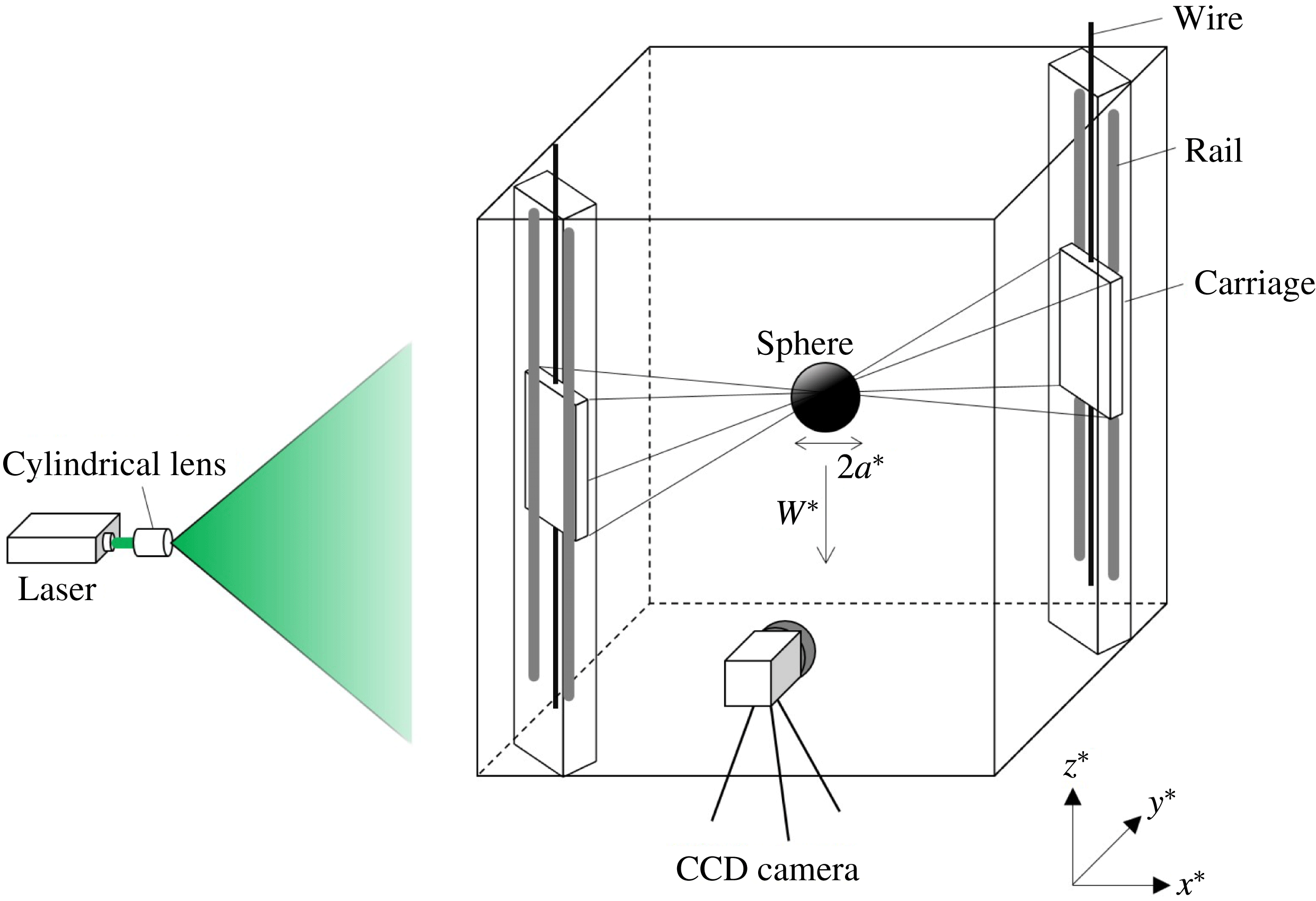
A schematic figure of the experimental facilities is presented in figure 2. The test tank, which has been used in the previous experiment (Hanazaki et al.
Reference Hanazaki, Kashimoto and Okamura2009a
), has a horizontal dimension of
 $80~\text{cm}\times 80~\text{cm}$
and a height of 94 cm. Linearly stratified salt water is filled up to the height of 88 cm using a two-tank method (Fortuin Reference Fortuin1960). To minimise the velocity disturbance generated when the fluid is pumped into the tank, a non-pulsating metering pump (Smoothflow Pump BPL-10-VTCF-FWS, TACMINA) is newly installed for the present experiment. Constant vertical gradient of the mean density
 $\bar{\unicode[STIX]{x1D70C}}^{\ast }(z^{\ast })$
is confirmed by a density meter (DMA 4500M, Anton Paar) whose accuracy is
 $5\times 10^{-5}~\text{g}~\text{cm}^{-3}$
.
An acrylic sphere of radius
 $a^{\ast }=2~\text{cm}$
is used, and it is sustained by eight stainless steel wires which span obliquely across the tank. The ends of the wires are connected to the four corners of the two rectangle carriage plates which move vertically along the rail. Two vertical rails are at the opposite corners of the tank, and a carriage on each rail is driven at a constant speed (
 $=$
sphere speed
 $W^{\ast }$
) by a high torque DC motor (Oriental motor BLHM450K-GFS) or by a brushless DC motor with a speed control system (Oriental motor BXS460A-50S-3). The latter motor was used for the measurement at low Reynolds numbers (
 $Re\leqslant 160$
) which requires the sphere speed less than
 $0.4~\text{cm}~\text{s}^{-1}$
. The effect of the sustaining wires on the flow would be negligible since the diameter of the wire (
 $=0.1~\text{mm}$
) is very thin as in the previous experiments (Hanazaki et al.
Reference Hanazaki, Kashimoto and Okamura2009a
).
The vertical light sheet for a planar PIV is generated using a double-pulsed Nd:YAG laser (Dual Power 65-15, Dantec Dynamics; Nano S PIV, Litron Lasers; 532 nm, 65 mJ, 15 Hz). Images of the seeding particles are photographed by a charge-coupled device (CCD) camera which has the resolution of 2048 pixel
 $\times$
2048 pixel (HiSense 4MC, Dantec Dynamics; C9300-024, Hamamatsu Photonics; 12 bits, 11 Hz). Two objective lenses with different focal lengths (AI Micro-Nikkor 105 mm f/2.8S and Nikkor 50 mm f/1.2) are used, depending on the area to be observed. Namely, when we observe the boundary layer along the sphere surface or the narrow cross-section of the jet, we have used the micro-lens of long focal length (
 $=$
105 mm) with a small angle of view, while when we observe a larger area in the lee of the sphere to identify the lee waves, we have used the lens of shorter focal length (
 $=$
50 mm) with a larger angle of view.
The coordinates used in this study are shown in figure 2. The
 $x^{\ast }$
-axis is in the horizontal direction of laser light and the
 $z^{\ast }$
-axis is in the vertical direction. The origin is located at the centre of the sphere and the coordinate frame goes down with the sphere at a constant speed (
 $=W^{\ast }$
). In this study,
 $w^{\ast }$
represents the vertical velocity relative to the sphere and
 $w^{\ast }-W^{\ast }$
(or
 $w-1$
in non-dimensional form) represents the vertical velocity in laboratory (stationary) frame.
A schematic figure of the experimental facilities. The origin of the coordinates is located at the centre of the sphere and moves downward with the sphere.

The flow is determined by the Froude number, Reynolds number and the Schmidt number, but the Schmidt number
 $Sc(=\unicode[STIX]{x1D708}^{\ast }/\unicode[STIX]{x1D705}^{\ast })$
(
 $\unicode[STIX]{x1D705}^{\ast }$
: diffusion coefficient of salinity) is constant throughout the experiments since we use salinity (
 $Sc\sim 700$
) to generate a stratified fluid. The Froude number and the Reynolds number are changed in the range of
 $0.4\leqslant Fr\leqslant 3.3$
and
 $110\leqslant Re\leqslant 550$
. All the physical quantities are hereafter non-dimensionalised by the length scale
 $2a^{\ast }(=4~\text{cm})$
, the velocity scale
 $W^{\ast }$
and the density scale
 $-2a^{\ast }\text{d}\bar{\unicode[STIX]{x1D70C}}^{\ast }/\text{d}z^{\ast }$
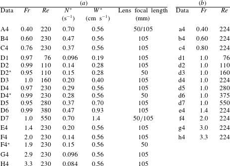
, and the variables without an asterisk denote non-dimensional quantities. The parameters are summarised in table 1(a). Since the generated stratified fluid often has a density gradient slightly different from the intended value, the realised values of
 $Fr$
and
 $Re$
are also slightly different from their intended values. This is the reason why the value of
 $Fr$
fluctuates around
 $Fr=1$
in table 1(a).
(a) The list of parameters used for the PIV experiments. For naming the data, we use letters (A–H) to represent the Froude numbers and numbers (1–7) to represent the Reynolds numbers, both in ascending order. The names with and without an asterisk (e.g. D2 and D2
 $^{\ast }$
) represent approximately the same but slightly different parameters. (b) The list of parameters used for the numerical simulations. The lower case letter (a–h) represent the Froude numbers and the numbers (1–7) represent the Reynolds numbers.

We observed the velocities on the
 $z$
axis, on the horizontal cross-section of the jet (
 $z=\text{const.}$
and
 $y=0$
) and on the
 $x$
axis in the boundary layer of the sphere. They were observed after the velocity field had become approximately stationary, i.e. for
 $W^{\ast }t^{\ast }/2a^{\ast }\gtrsim 10$
(cf. last paragraph of this section). Since the descending length of the sphere
 $(W^{\ast }t^{\ast })_{max}$
is less than the total fluid depth (
 $=$
88 cm) and is typically
 $(W^{\ast }t^{\ast })_{max}\sim 65~\text{cm}$
, the maximum non-dimensional time attainable in our test tank is
 $(W^{\ast }t^{\ast }/2a^{\ast })_{max}\sim 16$
when
 $2a^{\ast }=4$
cm. Therefore, PIV data observed in the period of
 $10\leqslant (W^{\ast }t^{\ast }/2a^{\ast })_{max}\leqslant 13$
are used in this study.
Since the camera remains stationary and the sphere moves downward, we need to know the position of each measurement point relative to the sphere. For this purpose, an accurate position of the centre of the sphere is necessary in every photograph. We measure the radius of the sphere in pixel unit when the sphere is stationary (within the error of two pixels), and use it to determine the centre of the sphere in each photograph. In general the measurement points of PIV do not coincide with the points which we intend to observe (e.g. points on the
 $z$
axis). Therefore, we obtain the velocity at the observation point by linear interpolation, using the velocity measured by PIV on the nearest four surrounding points. While the lens with a short focal length (
 $=$
50 mm) gives a non-dimensional spatial resolution of
 $\unicode[STIX]{x0394}x=\unicode[STIX]{x0394}z\simeq 9\times 10^{-2}$
, the lens with a long focal length (
 $=$
105 mm) gives a much higher resolution of
 $8\times 10^{-3}$
. Therefore, knowing that the radius of the jet and the boundary layer on the sphere surface both have a thickness of
 $O(0.1)$
(cf. figures 11 and 13 of § 3), use of the 105 mm lens would give sufficient resolution to observe these small areas and the errors due to interpolation would be negligible.
To reduce the effect of the experimental noise in the observed data, we averaged the velocities observed at the same point but at several successive times, knowing the steadiness of the actual flow in a short period. For example, when we observe the jet along the
 $z$
axis, the average is taken over every three to five frames (figures 7–9) while when we observe the horizontal cross-section of the jet (figures 10 and 11) or the boundary layer of the sphere (figures 12 and 13), we have averaged the velocity data from ten successive frames.
We have examined the reproducibility of the flow for a typical parameter
 $Re=230$
,
 $Fr=0.97$
(D4), and found that the vertical velocity in the jet (e.g. figure 10) observed on the same day but in another trial had differences of only less than a few per cent. This means that, after the random noises are eliminated by time averaging, the obtained data are highly reproducible.
In this study, numerical simulations have also been performed to simulate the flow at the Froude numbers and the Reynolds numbers nearly equal to those in the experiments. The list of parameters used for the numerical simulations are given in table 1(b). The non-dimensional parameters are the Froude number (
 $0.4\leqslant Fr\leqslant 3.3$
), Reynolds number (
 $76\leqslant Re\leqslant 550$
) and the Schmidt number which is fixed at
 $Sc=700$
. These simulations will allow a direct comparison with the experiments and will lead to a more complete discussion of the mechanisms of the flow.
The numerical method is exactly the same as Hanazaki et al. (Reference Hanazaki, Nakamura and Yoshikawa2015) in which a finite difference method combined with the body-fitting curvilinear coordinates was used. The governing equations are the Navier–Stokes equations with a buoyancy term under the Boussinesq approximation, transport equation of density and the divergence-free condition for the velocity. The convection terms of the Navier–Stokes equations and the density transport equations are approximated by a third-order upwind scheme and all the other spatial derivatives are approximated by central finite differences of second-order accuracy. The number of grid points is
 $360\times 1000$
, with 360 points in the direction along the sphere surface and 1000 points in the direction normal to the sphere surface. The grid spacing is small enough near the sphere surface where there is a thin density boundary layer whose thickness is estimated by
 $1/\sqrt{Re\,Sc}=1/\sqrt{550\times 700}=1.6\times 10^{-3}$
. In the present numerical grid, at least six grid points exist in this estimated thickness, although the actual density boundary layer is much thicker than this passive scalar limit (
 $Fr\rightarrow \infty$
, cf. Torres et al.
Reference Torres, Hanazaki, Castillo and Van Woert2000). In this study, an even finer mesh is used near the
 $z$
-axis, on which a thin vertical jet is generated and a large but local horizontal density variation is expected (cf. figure 2 of Hanazaki et al.
Reference Hanazaki, Nakamura and Yoshikawa2015).
Axisymmetry of the flow is assumed in all the simulated cases. In reality, the flow of a homogeneous fluid becomes asymmetric and has a circumferential flow around the vertical axis at Reynolds numbers above 200. Then, the results for
 $200<Re\leqslant 550$
might show some differences between the experiments and numerical simulations. However, the flows for the parameters investigated in this study preserve approximate axisymmetry in the experiments since the generation of the rear vortex is suppressed in stratified flows. This would justify the assumption of axisymmetry in numerical simulations. We should note that the jet in strongly stratified fluids begins to meander at some height above the sphere (cf. figure 1), but the flow remains axisymmetric just above the sphere until the meandering occurs. For example, in the case of
 $Re=200$
and
 $Fr=0.3$
, the meandering begins at a height of
 $z\sim 2.5$
. The beginning height of meandering changes with the parameters, but the height is usually proportional to the Froude number. Therefore, for the parameters investigated in this study (
 $Fr\geqslant 0.4$
), the flow would be nearly axisymmetric near the rear stagnation point (
 $z\lesssim 3$
). Possible effects of the asymmetry of the flow will be discussed later where appropriate (e.g. figures 7 and 8).
Throughout this study, the numerical results at time
 $t=10$
are used for comparison with the experiments so that the simulated time approximately agrees with the experiments. In our experiments the velocity distribution was essentially steady during the observation time (
 $10\leqslant t\leqslant 13$
), except for the effect of the noise. On the other hand, previous numerical simulations show that the unsteadiness remains for a longer time (
 $t>10$
) near the rear stagnation point and in the jet, but only for relatively large Froude numbers (
 $Fr\gtrsim 1$
, cf. figure 11 of Hanazaki et al.
Reference Hanazaki, Nakamura and Yoshikawa2015). In other regions, the velocity becomes steady much earlier, and the velocity boundary layer near the equator of the sphere (
 $z=0$
) is fully developed in a short time (typically
 $t\ll 5$
) and there is no unsteadiness for
 $t>10$
even for large Froude numbers (e.g.
 $Fr\geqslant 2$
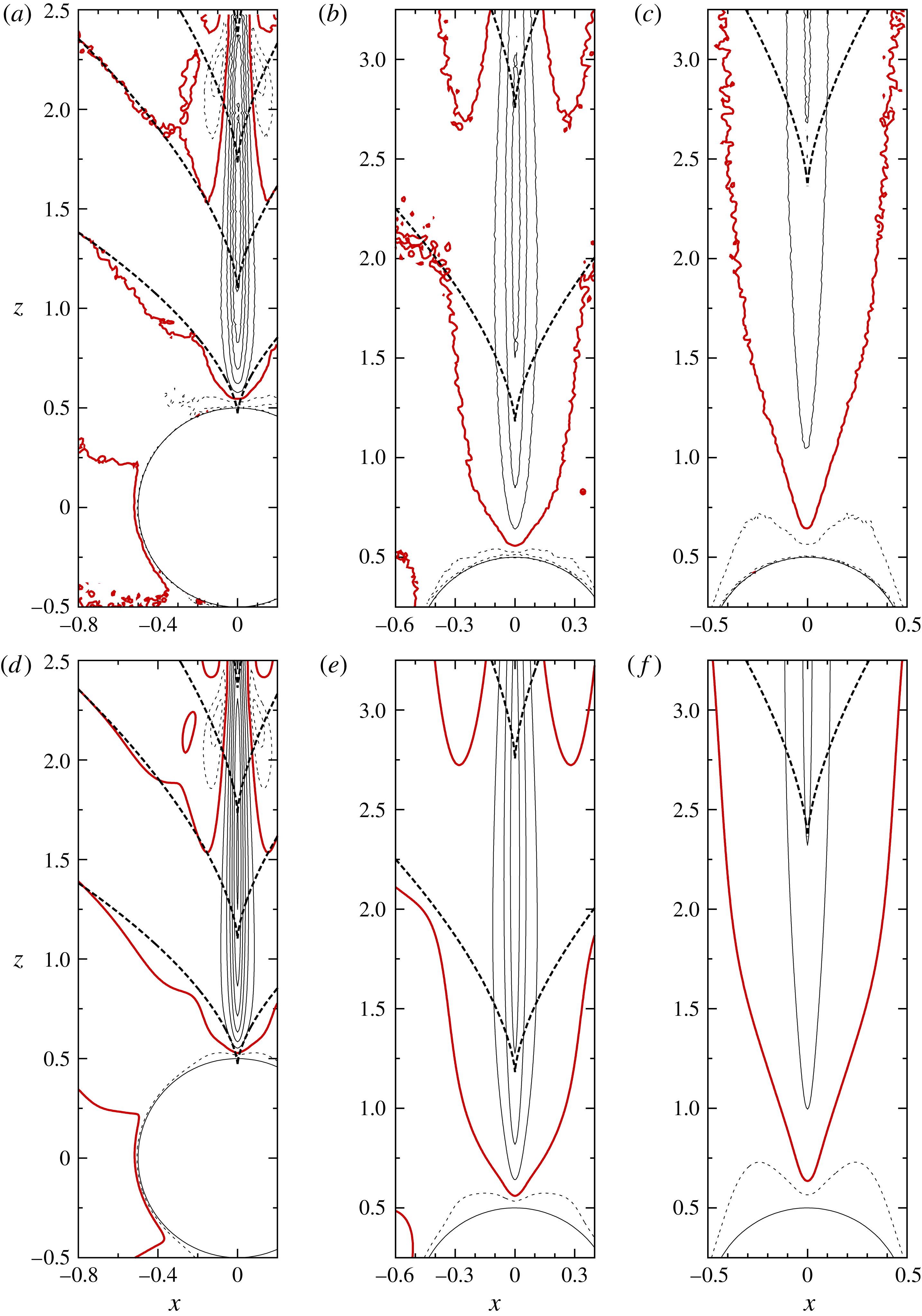
in figures 12 and 13). Then, the difference between the experiments and numerical simulations due to the time development of the flow may appear only in figures 3(c,f), 4(c,f), 7(a), 8, 10(a) and 11(a), where the numerical data in the jet are presented for
 $Fr>1$
. We will mention the effect of unsteadiness where it becomes appropriate, but the difference of the maximum velocity in the jet between
 $t=10$
and
 $t=13$
is approximately 3 % for
 $Fr=2$
and approximately 5 % for
 $Fr=3$
, and the effect of unsteadiness is generally small.
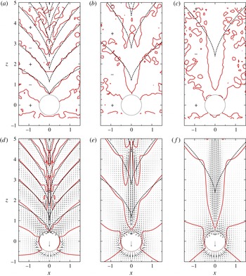
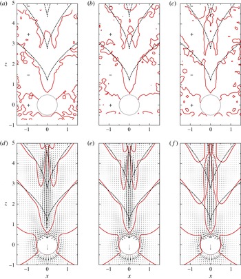
Froude number dependence of the distribution of vertical velocity in the vertical (
 $x{-}z$
) plane across the centre of the sphere. (a–c) Show the experimental results and (d–f) show the corresponding numerical results. The thick solid lines are the contours of zero vertical velocity (
 $w-1=0$
) and the dashed lines denote the same contours but obtained by linear theory using the method of stationary phase. In the experiments (a)
 $Fr=0.4$
(A4), (b)
 $Fr\sim 1.0$
(D4
 $^{\ast }$
) and (c)
 $Fr\sim 2.0$
(F4
 $^{\ast }$
), while the Reynolds number is fixed at
 $Re\sim 220$
and the lens of shorter focal length (
 $=$
50 mm) is used to obtain the overall images. Since the laser light comes from the left, measurement is impossible in the shadow region on the right of the sphere. Then, the contours in the shadow region are drawn using the data on the left side of the sphere, assuming axisymmetry of the flow. In numerical simulations, (d)
 $Fr=0.4$
(a4), (e)
 $Fr=1.0$
(d4) and (f)
 $Fr=2.0$
(f4), while the Reynolds number is fixed at
 $Re=224$
. The velocity vectors are also depicted and the downward arrow in the sphere shows the constant velocity of the sphere.

Close-up image of figure 3. (a–c) Show the experimental results for (a)
 $Fr=0.4$
(A4), (b)
 $Fr\sim 1.0$
(D4) and (c)
 $Fr\sim 2.0$
(F4), when the Reynolds number is fixed at
 $Re\sim 220$
. The lens of longer focal length (
 $=$
105 mm) is used here to obtain the close-up view. The contours of positive vertical velocity (
 $w-1=1,\ldots ,5$
) are shown by thin solid lines and the contours of negative vertical velocity (
 $w-1=-0.5,-1$
) near the rear stagnation point of the sphere are shown by thin dashed lines. (d–f) Show the numerical results for (d)
 $Fr=0.4$
(a4), (e)
 $Fr=1.0$
(d4) and (f)
 $Fr=2.0$
(f4), when the Reynolds number is fixed at
 $Re=224$
.

3 Results
We first show in figure 3(a–c) the Froude number dependence of the distribution of vertical velocity measured in the vertical (
 $x{-}z$
) plane across the centre of the sphere. The Froude number increases from left to right (
 $Fr=0.4$
, 1.0 and 2.0), while the Reynolds number is fixed at
 $Re\sim 220$
. The internal wave patterns are identified by the thick solid lines which show the contours of zero vertical velocity (
 $w-1=0$
) in the laboratory frame. The contours agree well between the experiments (a–c) and the numerical simulations (d–f) and show that the vertical velocity changes sign periodically in the vertical direction.
The dashed lines in figure 3 are the lines of
 $w-1=0$
obtained from the linear theory of internal waves using the method of stationary phase which is applicable to the far field. The lines of constant phase of the internal wave are given by Mowbray & Rarity (Reference Mowbray and Rarity1967) and Torres et al. (Reference Torres, Hanazaki, Castillo and Van Woert2000)
 $$\begin{eqnarray}\displaystyle & \displaystyle r^{\ast }/2a^{\ast }=\frac{1}{2}Fr\unicode[STIX]{x1D6F7}\left(\frac{(\unicode[STIX]{x1D70E}^{-4}+\unicode[STIX]{x1D70E}^{-2}-1)(1-\unicode[STIX]{x1D70E}^{2})^{3}}{(1-\unicode[STIX]{x1D70E}^{2})^{3}+\unicode[STIX]{x1D70E}^{2}(2-\unicode[STIX]{x1D70E}^{2})^{2}}\right)^{1/2}, & \displaystyle\end{eqnarray}$$
 $$\begin{eqnarray}\displaystyle & \displaystyle z^{\ast }/2a^{\ast }=\frac{1}{2}Fr\unicode[STIX]{x1D6F7}\unicode[STIX]{x1D70E}(2-\unicode[STIX]{x1D70E}^{2})\left(\frac{\unicode[STIX]{x1D70E}^{-4}+\unicode[STIX]{x1D70E}^{-2}-1}{(1-\unicode[STIX]{x1D70E}^{2})^{3}+\unicode[STIX]{x1D70E}^{2}(2-\unicode[STIX]{x1D70E}^{2})^{2}}\right)^{1/2}, & \displaystyle\end{eqnarray}$$
where
 $r^{\ast }$
is the horizontal distance from the
 $z$
-axis,
 $\unicode[STIX]{x1D70E}$
(
 $0<\unicode[STIX]{x1D70E}<1$
) is a variable parameter,
 $\unicode[STIX]{x1D6F7}$
is the phase of the internal wave and
 $\unicode[STIX]{x1D6F7}=(n-1/4)\unicode[STIX]{x03C0}$
(
 $n=1,2,\ldots$
) corresponds to
 $w-1=0$
. The lee wave patterns of
 $w-1=0$
obtained by (3.1) and (3.2) agree well with the experiments and numerical simulations, especially for the far field.
In figure 3(d–f), a region of large vertical velocity, i.e. a ‘jet’, is identified along the symmetry axis (
 $z$
axis) of the flow. The vertical distance between the contours of zero vertical velocity (
 $w-1=0$
) shows that the jet length is shortest at the lowest Froude number (
 $Fr=0.4$
), i.e. under the strongest stratification. The relation between the length of the jet and the wavelength of the internal waves has been discussed in previous numerical simulations (Hanazaki et al.
Reference Hanazaki, Nakamura and Yoshikawa2015, figures 8 and 9), but the velocity distributions have yet to be measured in the experiments, particularly to identify the Froude number dependence. Present results show the increase of wavelength/jet length with the Froude number clearly.
Figure 4 shows the close-up image of the velocity distribution. Figure 4(a–c) shows the contours of vertical velocity obtained by experiments using the lens of long focal length (
 $=$
105 mm). The experiments and the numerical simulations (figure 4
d–f) are in good agreement, and the largest velocity appears between the first and the second line of
 $w-1=0$
encountered when we go upward from the upper stagnation point of the sphere (
 $(x,z)=(0,0.5)$
). We note also that the maximum vertical velocity in the jet is larger for smaller
 $Fr$
(cf. figure 7).
We note some differences in the thick solid lines near the
 $z$
axis between figures 3(a) and 4(a). While the time interval between the laser pulses is set to be large in figure 3(a–c) in order to observe the slow motion due to the internal gravity waves, the long time interval is not suitable for the observation of the fast flow in the jet. Then, the velocity data in figure 3(a–c) are significantly less accurate in the jet region.
It should be noted that the above theoretical results (3.1) and (3.2) are derived for the inviscid and non-diffusive fluid and do not include viscous or diffusive effects. On the other hand, the buoyant jet has its origin in the molecular diffusion of density which violates the conservation of density (Hanazaki et al.
Reference Hanazaki, Nakamura and Yoshikawa2015), and it will appear regardless of the existence of the internal waves. Therefore, the flow just above the sphere, where a strong jet exists, might not be well described by (3.1) and (3.2). Only if the vertical position becomes higher (
 $z^{\ast }/(2a^{\ast })\gg 1$
) and the effect of the jet becomes weaker will the theory become accurate. However, we can still say that the jet would be strongly affected by the lee waves even near the sphere (
 $z^{\ast }/(2a^{\ast })\lesssim 1$
), since the flow just outside the jet is determined by the internal waves. Indeed, the unique bell-shaped structure appears (figure 1) where the downward velocity due to the internal wave becomes maximum (Hanazaki et al.
Reference Hanazaki, Nakamura and Yoshikawa2015). Then, the vertical length of the jet might also be significantly affected by the points of zero vertical velocity (
 $w-1=0$
) on the
 $z$
axis, which are predicted by (3.1) and (3.2).
It is clear in numerical simulations (figures 3 d–f and 4 d–f) that the radius of the round jet becomes larger for larger Froude numbers, while the same tendency can be observed also in the experiments (in figure 4 a–c). The downward flow around the jet in figures 3(d,e) and 4(d) corresponds to the bell-shaped structure observed by the shadowgraph method (figure 1).
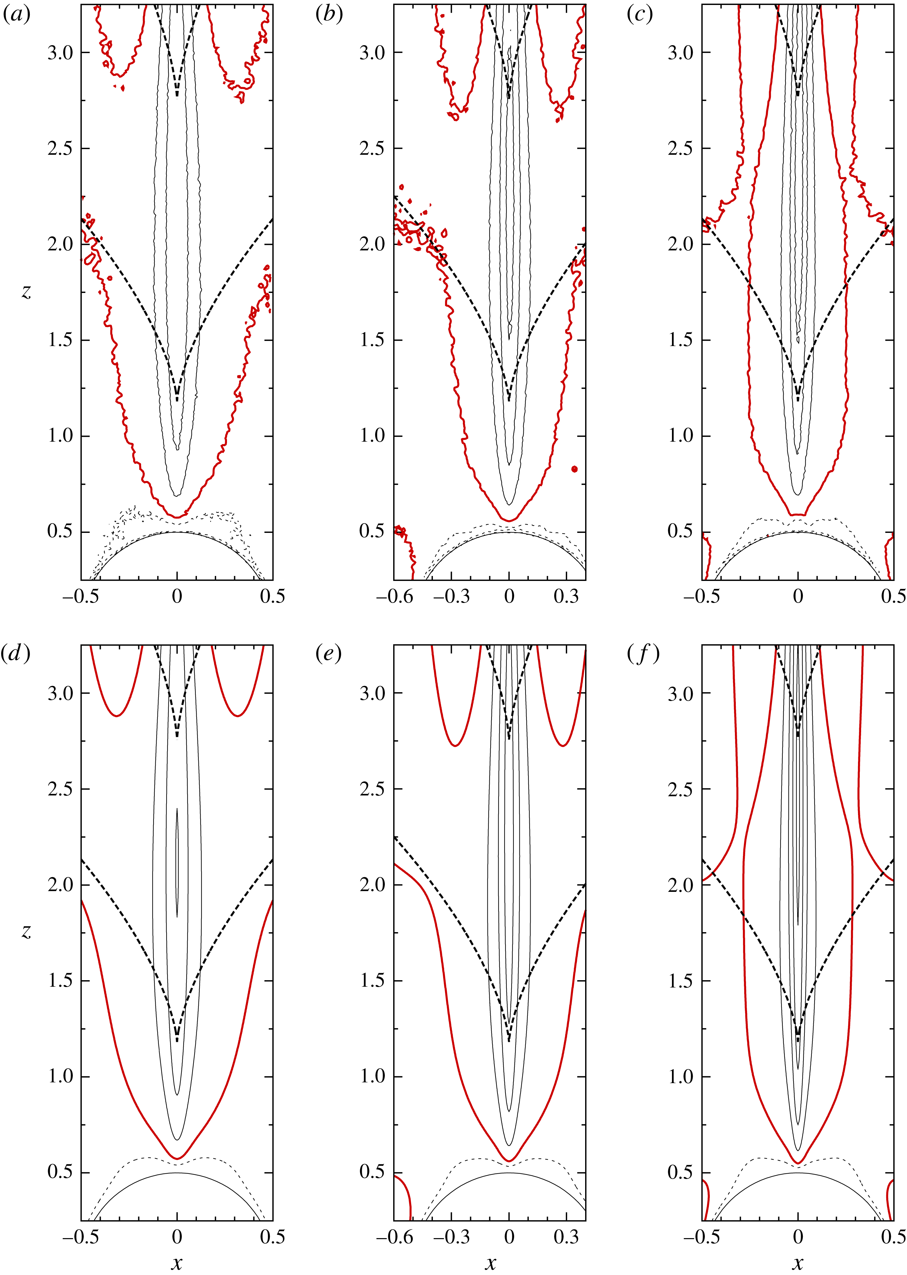
We next investigate in figures 5 and 6 the Reynolds number dependence of the flow at a fixed Froude number (
 $Fr\sim 1.0$
). The contours of zero vertical velocity change only slightly as the Reynolds number increases from 110 to 550. The wavelength of an internal wave does not depend on viscosity and is independent of the Reynolds number. On the other hand, the radius of the jet becomes narrower for larger Reynolds numbers since it is comparable to the boundary-layer thickness which becomes thinner for larger Reynolds numbers. This has been predicted by numerical simulations (Hanazaki et al.
Reference Hanazaki, Nakamura and Yoshikawa2015), but the present experiment confirms it in the real fluid.
Reynolds number dependence of the distribution of vertical velocity in the vertical (
 $x{-}z$
) plane across the centre of the sphere. (a–c) Show the experimental results for (a)
 $Re=110$
(D2
 $^{\ast }$
), (b)
 $Re=230$
(D4
 $^{\ast }$
) and (c)
 $Re=550$
(D7), when the Froude number is fixed at
 $Fr\sim 1$
. The lens of shorter focal length (
 $=$
50 mm) is used to obtain the overall images. (d–f) Show the numerical results for (d)
 $Re=110$
(d2), (e)
 $Re=224$
(d4) and (f)
 $Re=550$
(d7), when the Froude number is fixed at
 $Fr=1$
. Captions for the lines and arrows are the same as figure 3.

Close-up image of figure 5. (a–c) Show the experimental results for (a)
 $Re=110$
(D2), (b)
 $Re=230$
(D4) and (c)
 $Re=550$
(D7), when the Froude number is fixed at
 $Fr\sim 1$
. The lens of longer focal length (
 $=105$
mm) is used here to obtain the close-up view. (d–f) Show the numerical results for (d)
 $Re=110$
(d2), (e)
 $Re=224$
(d4) and (f)
 $Re=550$
(d7), when the Froude number is fixed at
 $Fr=1$
. Captions for the lines are the same as in figure 4.

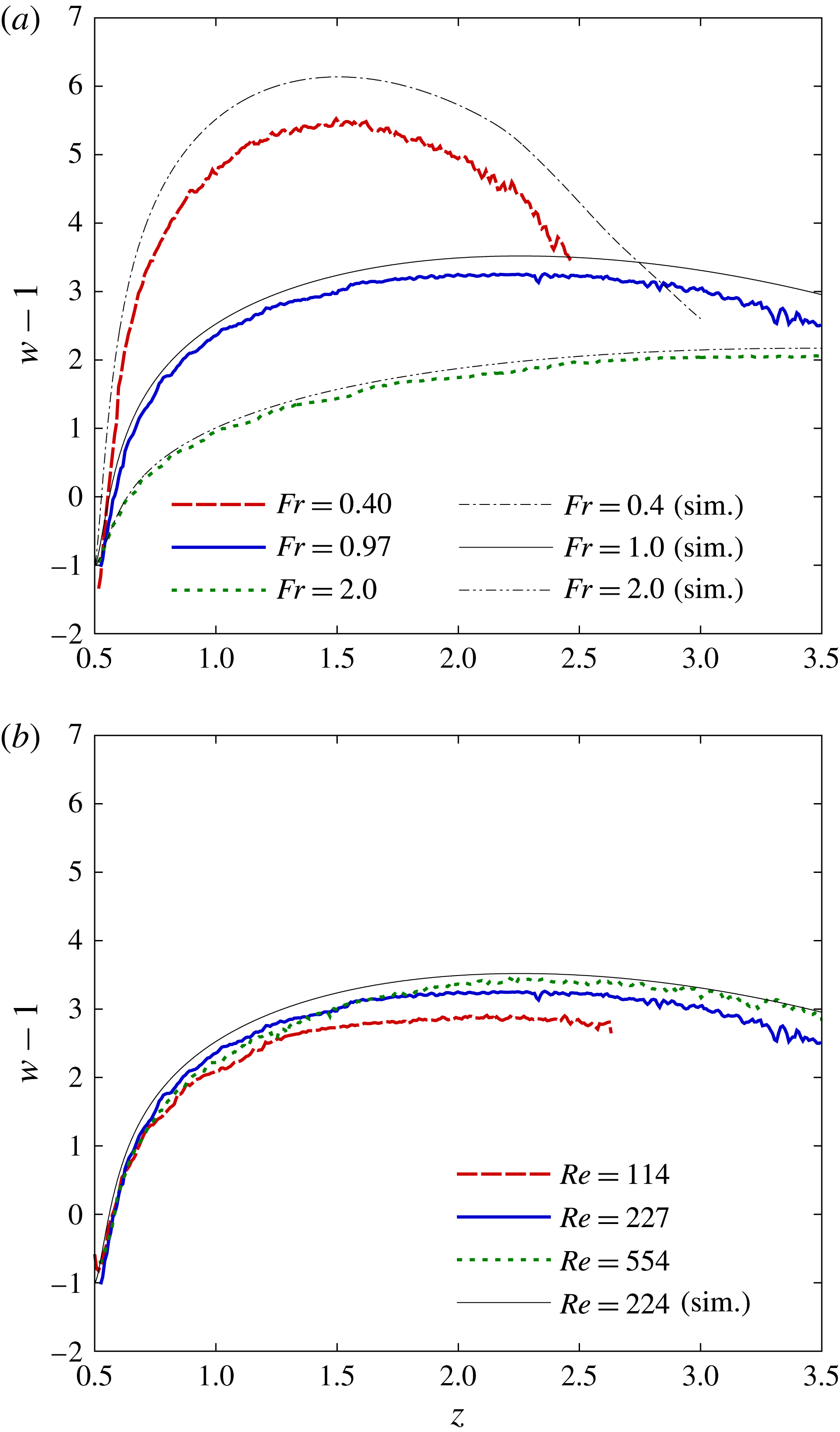
Figure 7 shows the distributions of vertical velocity on the symmetry axis (
 $z$
axis) of the flow. In figure 7(a) the Froude number is changed from 0.4 to 2.0 while the Reynolds number is fixed at
 $Re\sim 220$
. The maximum velocity (
 $(w-1)_{max}\sim 5.4$
) is observed at the lowest Froude number (
 $Fr=0.4$
) and it decreases with increasing Froude number, corresponding to the increase of the jet radius. Results of PIV and numerical simulations show a qualitative agreement. At
 $Re\sim 220$
, the whole flow field is axisymmetric in experiments for weak stratifications (
 $Fr\gtrsim 1$
), while an asymmetric meandering of the jet appears far above the sphere for low Froude numbers (
 $Fr\lesssim 1$
, cf. figure 1). In the present study, meandering of the jet appears for
 $z\gtrsim 3$
in the case of
 $Fr=0.4$
, and those fluctuations, although small below
 $z\sim 3$
, would partly explain the smaller vertical velocity in the experiment than that in the numerical simulation, since the axisymmetry is assumed only in the numerical simulation. Another possible explanation is that the laser light sheet has a finite thickness in the horizontal direction, and the area observed by PIV includes the region around the
 $z$
axis where the vertical velocity is smaller than the velocity exactly on the
 $z$
axis. In figure 7(a) we note also that the maximum velocity occurs at a higher position for a larger Froude number, corresponding to the larger vertical wavelength of the internal wave.
In figure 7(b), the Reynolds number is changed from 110 to 550 while the Froude number is fixed at
 $Fr\sim 1.0$
. The dependence of the vertical velocity on the Reynolds number is relatively weak, but the maximum velocity is larger for a larger Reynolds number. This is consistent with figure 6, since the narrower radius of the jet will lead to a faster vertical velocity if the total flow rate in the jet is the same. The larger velocity at larger Reynolds number can be explained also by the smaller viscous dissipation.
Distributions of the vertical velocity in laboratory frame (i.e.
 $w-1$
) on the
 $z$
-axis, where
 $z=0.5$
is the upper/downstream stagnation point of the sphere. (a) Froude number is changed from
 $Fr=0.4$
to 2.0, while the Reynolds number is fixed at
 $Re\sim 220$
. The results of PIV (A4, D4, F4) and numerical simulations (a4, d4, f4). (b) Reynolds number is changed from
 $Re=110$
to 550, while the Froude number is fixed at
 $Fr\sim 1.0$
. The results of PIV (D2, D4, D7) and a numerical simulation (d4).

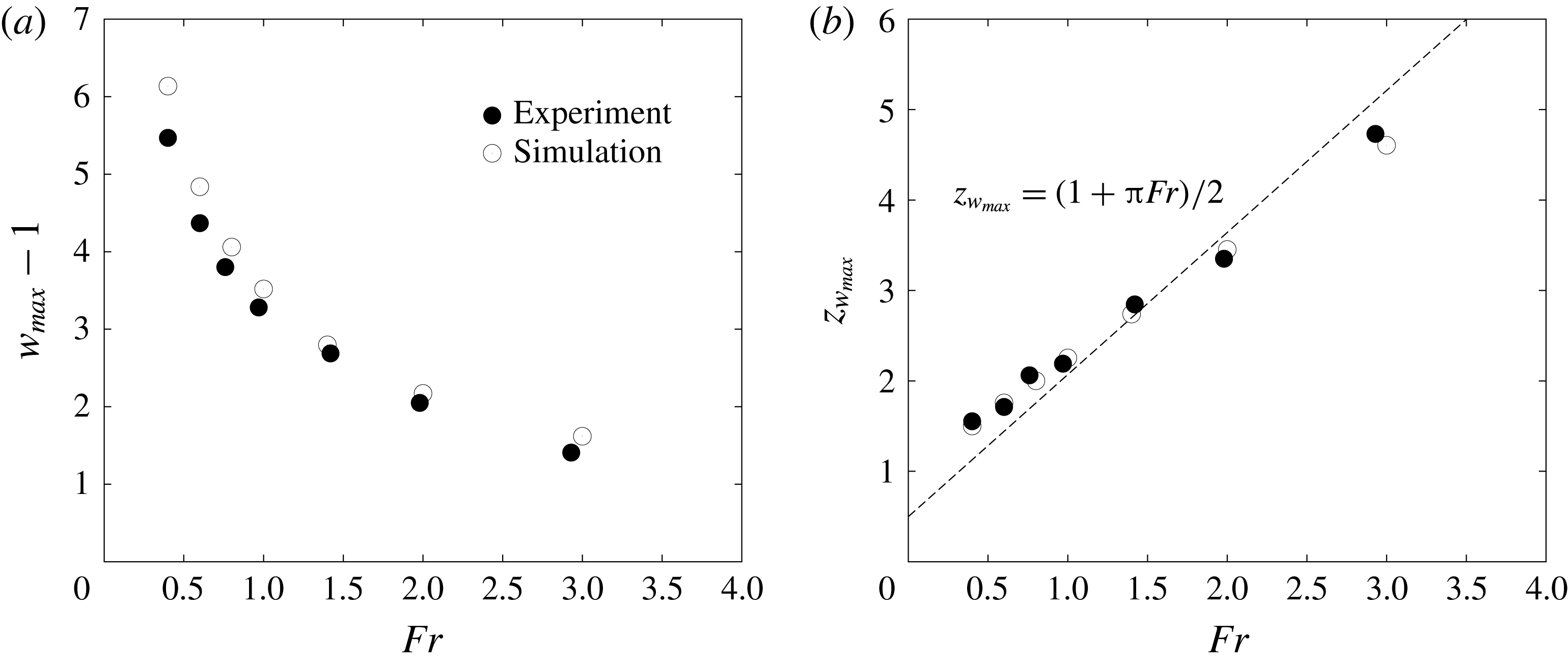
The maximum vertical velocity
 $w_{max}$
and the height at which it appears (
 $z_{w_{max}}$
) are shown in figure 8 against seven values of
 $Fr$
, but for a fixed Reynolds number (
 $Re\sim 220$
). In figure 8(a), the maximum velocity decreases with
 $Fr$
as observed in figure 7(a), and satisfies roughly
 $(w_{max}-1)\propto Fr^{-1/2}$
for small Froude numbers (
 $Fr\lesssim 1$
). This becomes clear when we plot in a double logarithmic chart, although the result is not provided here. We note also that the numerical simulations give maximum velocities larger than the experiments at low Froude numbers. This would be explained possibly by the weak three-dimensionality of the jet at low Froude numbers (
 $Fr\lesssim 1$
) and by the thickness of the laser light sheet, as in figure 7(a). Since the jet becomes narrower for smaller Froude numbers while the thickness of the laser light sheet is constant, the difference between the measured maximum velocity and the real maximum velocity exactly on the
 $z$
axis would become larger as the Froude number decreases. This tendency is actually observed in figure 8(a). We should mention that the difference between the experiments and numerical simulations cannot be explained by the time development of the flow between
 $t=10$
and
 $t=13$
, since the simulated velocity would slightly increase between
 $t=10$
and
 $t=13$
for large Froude numbers (
 $Fr\gtrsim 2$
) and the difference would become even larger.
Froude number dependence of (a) the maximum vertical velocity
 $w_{max}-1$
and (b) the vertical coordinate
 $z_{w_{max}}$
at which the vertical velocity becomes maximum. The Reynolds number is fixed at
 $Re\sim 220$
. The results of PIV (A4–G4) and numerical simulations (a4–g4) are presented.

In figure 8(b), the height at which the vertical velocity becomes maximum (
 $z_{w_{max}}$
) increases in proportion to
 $Fr$
. In a numerical study (Hanazaki et al.
Reference Hanazaki, Nakamura and Yoshikawa2015), the vertically dragged length of the fluid by the sphere has been found to be
 $$\begin{eqnarray}L^{\ast }=2\unicode[STIX]{x03C0}W^{\ast }/N^{\ast }=2\unicode[STIX]{x03C0}Fra^{\ast }\quad (\text{for}\;Fr\gtrsim 1),\end{eqnarray}$$
which agrees with the vertical wavelength of the internal wave. Since the estimation
 $2\unicode[STIX]{x03C0}W^{\ast }/N^{\ast }$
does not contain the sphere radius
 $a^{\ast }$
, we can expect that the dimensional dragged length of the fluid is determined only by the stratification and the vertical velocity of the obstacle, and not by the obstacle size. Equation (3.3) can be rewritten in non-dimensional form as
 $$\begin{eqnarray}L^{\ast }/2a^{\ast }=\unicode[STIX]{x03C0}Fr\quad (Fr\gtrsim 1).\end{eqnarray}$$
If we assume that the fluid in the jet has a small vertical velocity when it returns to its original height, the maximum velocity would occur approximately midway between the rear (i.e. upper) stagnation point of the sphere and the original height of the fluid. Then, the maximum velocity would appear at the non-dimensional vertical coordinate of
 $$\begin{eqnarray}z_{w_{max}}^{\ast }/2a^{\ast }\simeq (1+\unicode[STIX]{x03C0}Fr)/2\quad (Fr\gtrsim 1),\end{eqnarray}$$
where
 $1/2$
on the right-hand side is the height of the rear stagnation point of the sphere. This is a bold estimation, but it agrees fairly well with the experiments and numerical simulations. While the formation of a jet cannot be explained directly by the internal wave, its wavelength determines one of the important aspects of the jet. We note that the dimensional distance between the point of maximum velocity and the rear stagnation point, i.e.
 $z_{w_{max}}^{\ast }-a^{\ast }=\unicode[STIX]{x03C0}W^{\ast }/N^{\ast }$
, does not depend on
 $a^{\ast }$
, showing that it is also independent of the size of the obstacle.
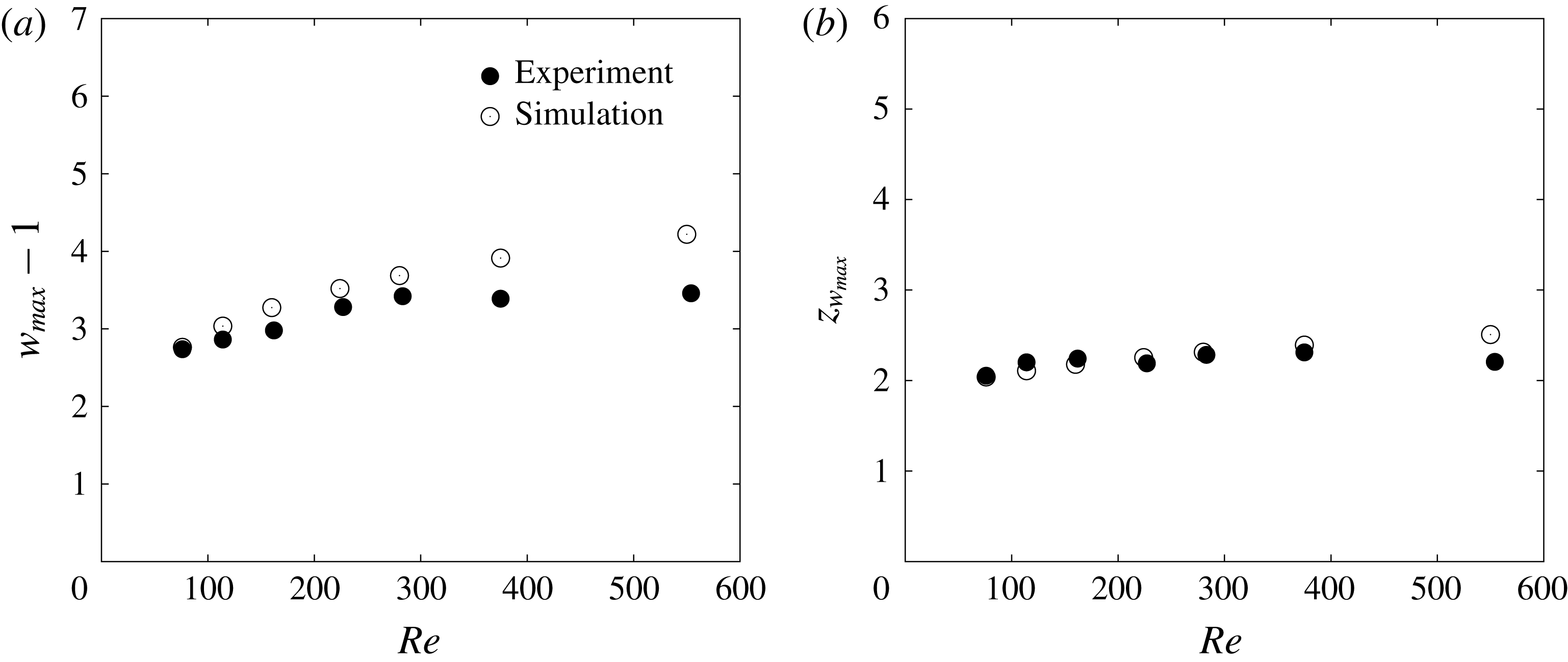
Reynolds number dependence of (a) the maximum vertical velocity
 $w_{max}-1$
and (b) the vertical coordinate at which the maximum vertical velocity is observed (
 $z_{w_{max}}$
). The Froude number is fixed at
 $Fr\sim 1.0$
. The results of PIV (D1–D7) and numerical simulations (d1–d7) are presented.

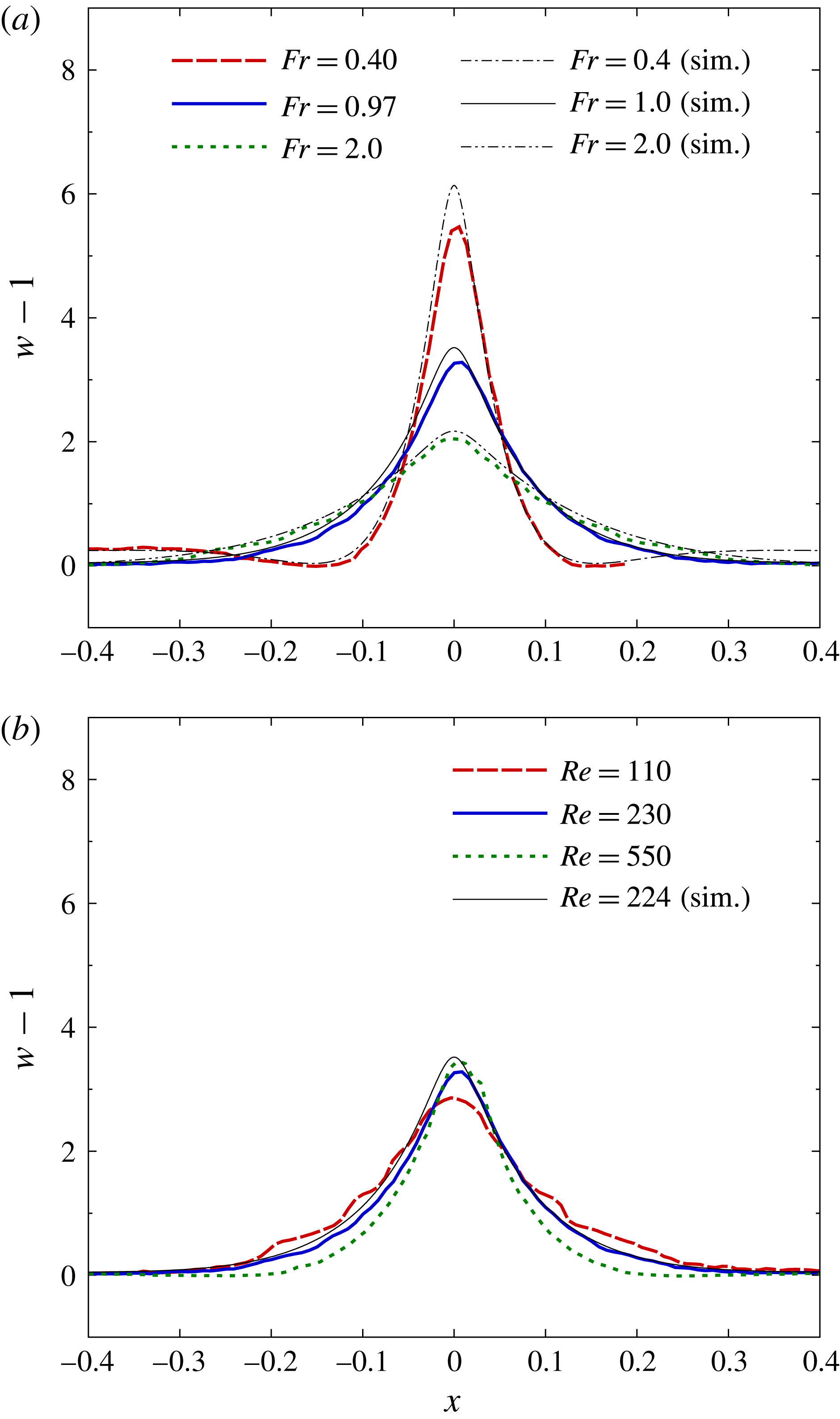
Distributions of the vertical velocity on the horizontal plane at
 $z=z_{w_{max}}$
. (a) Froude number dependence at a fixed Reynolds number (
 $Re\sim 220$
), obtained from PIV (A4, D4, F4) and numerical simulations (a4, d4, f4). (b) Reynolds number dependence at a fixed Froude number (
 $Fr\sim 1.0$
), obtained from PIV (D2, D4, D7) and numerical simulations (d4).

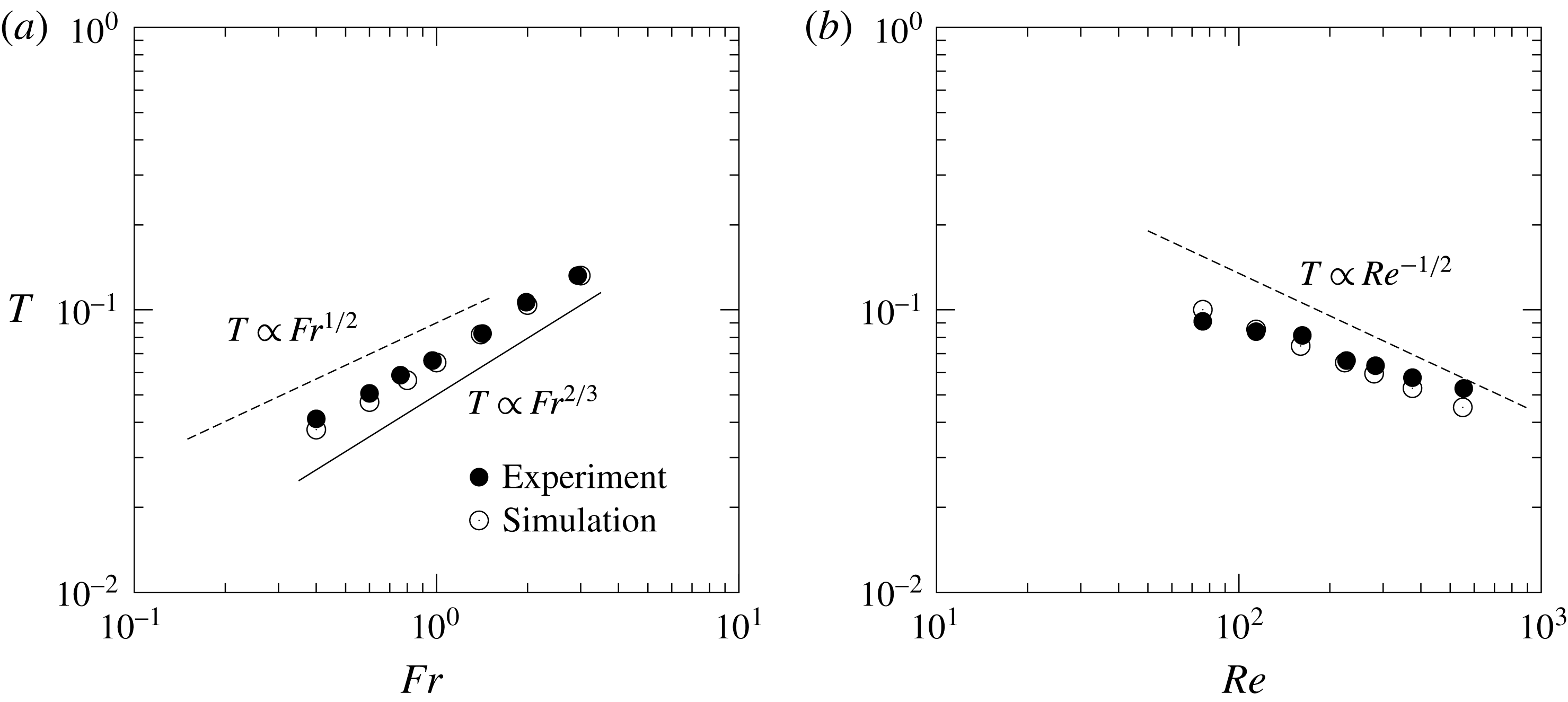
(a) Froude number dependence of the jet radius
 $T$
at
 $Re\sim 220$
, obtained from PIV (A4–G4) and numerical simulations (a4–g4). (b) Reynolds number dependence of the jet radius
 $T$
at
 $Fr\sim 1.0$
, obtained from PIV (D1–D7) and numerical simulations (d1–d7). Dashed lines show the estimation given by (3.8), which is proportional to
 $Fr^{1/2}$
(
 $Fr\lesssim 1$
) for a constant
 $Re$
(a) and proportional to
 $Re^{-1/2}$
for a constant
 $Fr$
(b). Solid line in (a) shows the proportionality of the wake width to
 $Fr^{2/3}$
, which could be inferred from the numerical results by Yick et al. (Reference Yick, Torres, Peacock and Stocker2009) at low
 $Re({\leqslant}0.5)$
.

The variation of the maximum vertical velocity
 $w_{max}$
and the height at which it appears (
 $z_{w_{max}}$
) are shown in figure 9 against seven Reynolds numbers (
 $80\leqslant Re\leqslant 550$
), while the Froude number is fixed at
 $Fr\sim 1$
. In figure 9(a) the maximum vertical velocity slightly increases with the Reynolds number, probably due to the narrower jet and the weaker viscosity effect at higher Reynolds numbers. The experiments and the numerical simulations show good agreement at low Reynolds numbers (
 $80\leqslant Re\lesssim 200$
), i.e. when the flow is nearly axisymmetric. Overestimation by the numerical simulations at higher Reynolds numbers (
 $Re>200$
) may be due to the assumption of axisymmetry, since the generation of circumferential velocity around the
 $z$
axis in a real three-dimensional flow would reduce the vertical component of the flow, although the circumferential component is not measured in this study. The height for which the maximum velocity appears (figure 9
b) is almost independent of the Reynolds number, since
 $z_{w_{max}}$
would be determined essentially by the vertical wavelength of the internal wave, which is proportional to the Froude number. In figure 9(b) the experiments show better agreement with the numerical simulations than in figure 9(a), since the weak three-dimensionality of the flow would not affect the vertical wavelength of the internal wave.
Figure 10 shows the distribution of vertical velocity on the horizontal line located at the height of the maximum vertical velocity (
 $z=z_{w_{max}}$
and
 $y=0$
). In figure 10(a), dependence on the Froude number (
 $0.4\leqslant Fr\leqslant 2$
) is shown when the Reynolds number is fixed at
 $Re\sim 220$
. We observe that the jet becomes slower with increasing
 $Fr$
, in agreement with figures 7(a) and 8(a). In figure 10(b), the Reynolds number is changed (
 $110\leqslant Re\leqslant 550$
) while the Froude number is fixed at
 $Fr\sim 1$
. This figure shows that the velocity distribution is not strongly affected by
 $Re$
, but the peak velocity slightly increases and the jet becomes thinner as the Reynolds number increases (cf. figures 7
b, 9
a).
We next discuss the radius of the jet, which is defined by the half-width at half maximum in the distribution of
 $w-1$
on the horizontal plane of
 $z=z_{w_{max}}$
. In figure 11(a), the jet radius non-dimensionalised by
 $2a^{\ast }$
is denoted by
 $T$
and is plotted against seven values of
 $Fr$
for a fixed
 $Re({\sim}220)$
. In figure 11(b), it is plotted against seven values of
 $Re$
for a fixed
 $Fr({\sim}1)$
. In a previous paper on numerical simulations (Hanazaki et al.
Reference Hanazaki, Nakamura and Yoshikawa2015), it has been found that the primitive length scale in stratified fluid (Gibson Reference Gibson and Nihoul1980; Yick et al.
Reference Yick, Torres, Peacock and Stocker2009)
 $$\begin{eqnarray}l_{\unicode[STIX]{x1D708}}^{\ast }=\sqrt{\unicode[STIX]{x1D708}^{\ast }/N^{\ast }}=\left(\frac{2a^{\ast 2}Fr}{Re}\right)^{1/2},\end{eqnarray}$$
which can be non-dimensionalised by the sphere diameter
 $2a^{\ast }$
as
 $$\begin{eqnarray}\frac{l_{\unicode[STIX]{x1D708}}^{\ast }}{2a^{\ast }}=\left(\frac{Fr}{2Re}\right)^{1/2},\end{eqnarray}$$
becomes the typical length scale for the velocity boundary-layer thickness on the sphere surface. Since the thickness of the velocity boundary layer should asymptote to
 $\sqrt{1/Re}$
in a homogeneous fluid (
 $Fr\rightarrow \infty$
), equation (3.7) would hold only for sufficiently small
 $Fr({\lesssim}1)$
. We would expect the agreement between the boundary-layer thickness and the jet radius since the jet is a continuation of the boundary layer on the sphere. Then, the jet radius would be estimated similarly by
 $$\begin{eqnarray}T\sim \frac{l_{\unicode[STIX]{x1D708}}^{\ast }}{2a^{\ast }}=\left(\frac{Fr}{2Re}\right)^{1/2},\end{eqnarray}$$
again for small
 $Fr({\lesssim}1)$
. This expression includes two proportionality relations, i.e.
 $$\begin{eqnarray}T\propto Fr^{1/2},\end{eqnarray}$$
for a constant
 $Re$
, and
 $$\begin{eqnarray}T\propto Re^{-1/2},\end{eqnarray}$$
for a constant
 $Fr$
, both under the condition of
 $Fr\lesssim 1$
. The former relation (3.9) is approximately observed in figure 11(a), and the latter relation (3.10) is observed in figure 11(b), with a good agreement between experiments and numerical simulations. In figure 11(a) the proportionality in the log–log plot should be expected only for low Froude numbers (
 $Fr\lesssim 1$
), but the experimental results show that it would actually be extended to higher Froude numbers (
 $Fr\gtrsim 1$
). It should be noted that figure 11(b) shows the case of
 $Fr\sim 1$
for which the relation (3.10) would hold only marginally, so the proportionality in the log–log plot might become better for lower
 $Fr$
.
We may consider how the width of the jet changes when the Reynolds number is reduced from
 $Re=O(10^{2})$
. According to Yick et al. (Reference Yick, Torres, Peacock and Stocker2009), the buoyant jet behind the sphere is not generated at low Reynolds numbers (
 $Re\lesssim 1$
), although a weak vertical flow is discernible in their figure 8(c), and only the vertical deflection of isopycnals is observed in the wake of the sphere. The width of the wake determined by the deflection of isopycnals is typically larger than the radius of the sphere, and they argued that it is proportional to
 $Ri^{-1/3}$
where
 $Ri=Re/Fr^{2}$
is the viscous Richardson number. In their figure 12(a) the width looks proportional to
 $Ri^{-1/3}$
, but the proportionality constant is different for different
 $Re$
, meaning that the width would be actually described by
 $C(Re)Ri^{-1/3}(=C(Re)Re^{-1/3}Fr^{2/3})$
, where
 $C(Re)$
is a function of
 $Re$
. Then, the width is proportional to
 $Fr^{2/3}$
for a constant
 $Re$
, but its dependence on
 $Re$
and
 $Ri$
is uncertain in their figures. It might be of some interest, however, to note that the jet radius
 $T$
in our figure 11(a) is proportional to
 $Fr$
raised to the power of
 $1/2$
or
 $2/3$
, and
 $Fr^{2/3}$
seems to be a good approximation, although the jet and wake have different flow structures with a significantly different width, and the Reynolds number is much higher in the present study.
Distributions of the vertical velocity
 $w-1$
on the
 $x$
axis outside the sphere (i.e.
 $x=-0.5-d$
(
 $d\geqslant 0$
)), where
 $d$
is the distance from the sphere surface. (a) Froude number dependence at
 $Re\sim 220$
, obtained from PIV (A4, D4, F4) and numerical simulations (a4, d4, f4). The boundary-layer thickness
 $\unicode[STIX]{x1D6FF}$
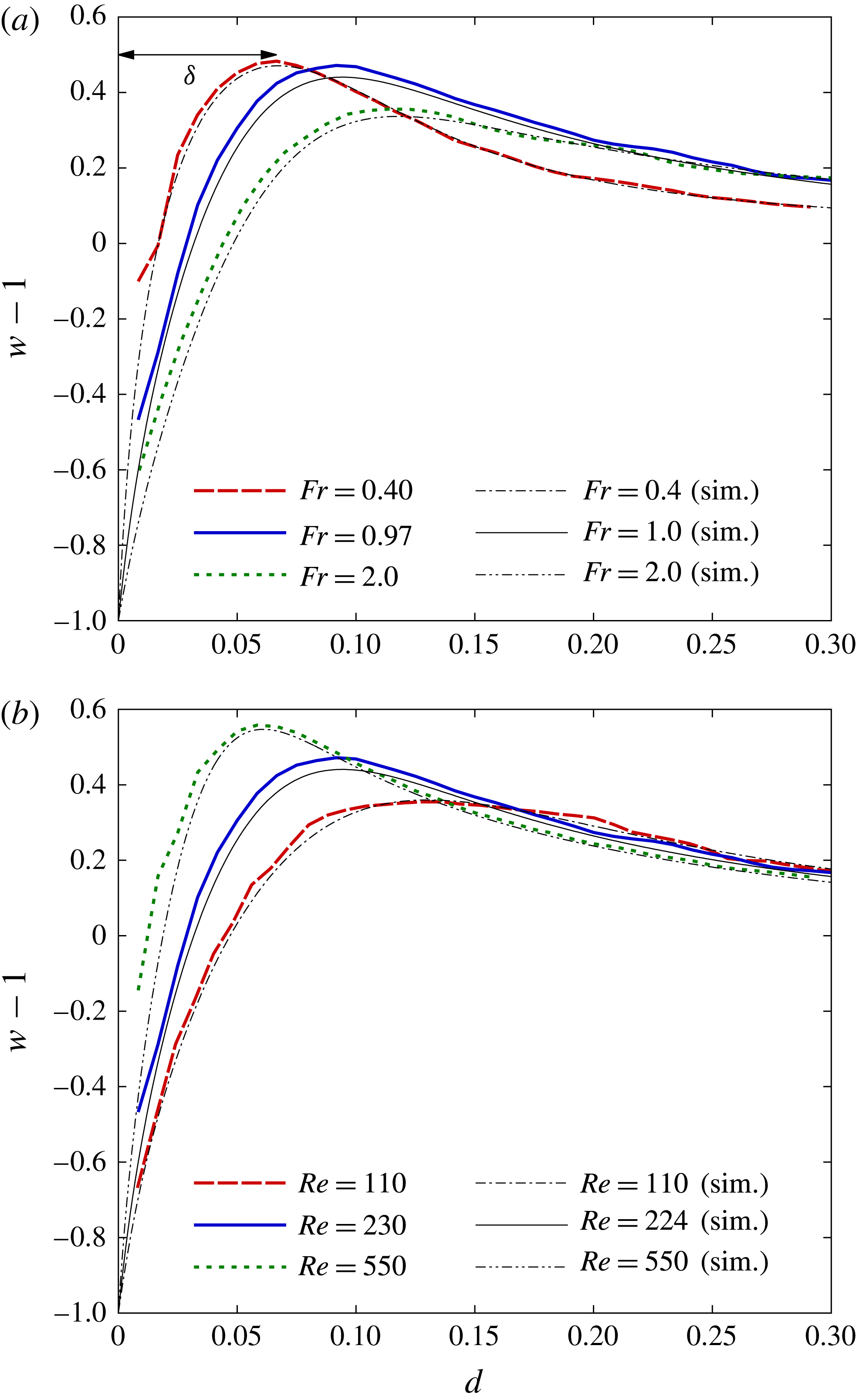
is determined by the distance of the peak position of vertical velocity from the sphere surface, as indicated in figure 12(a). (b) Reynolds number dependence at
 $Fr\sim 1.0$
, obtained from PIV (D2, D4, D7) and numerical simulations (d2, d4, d7).

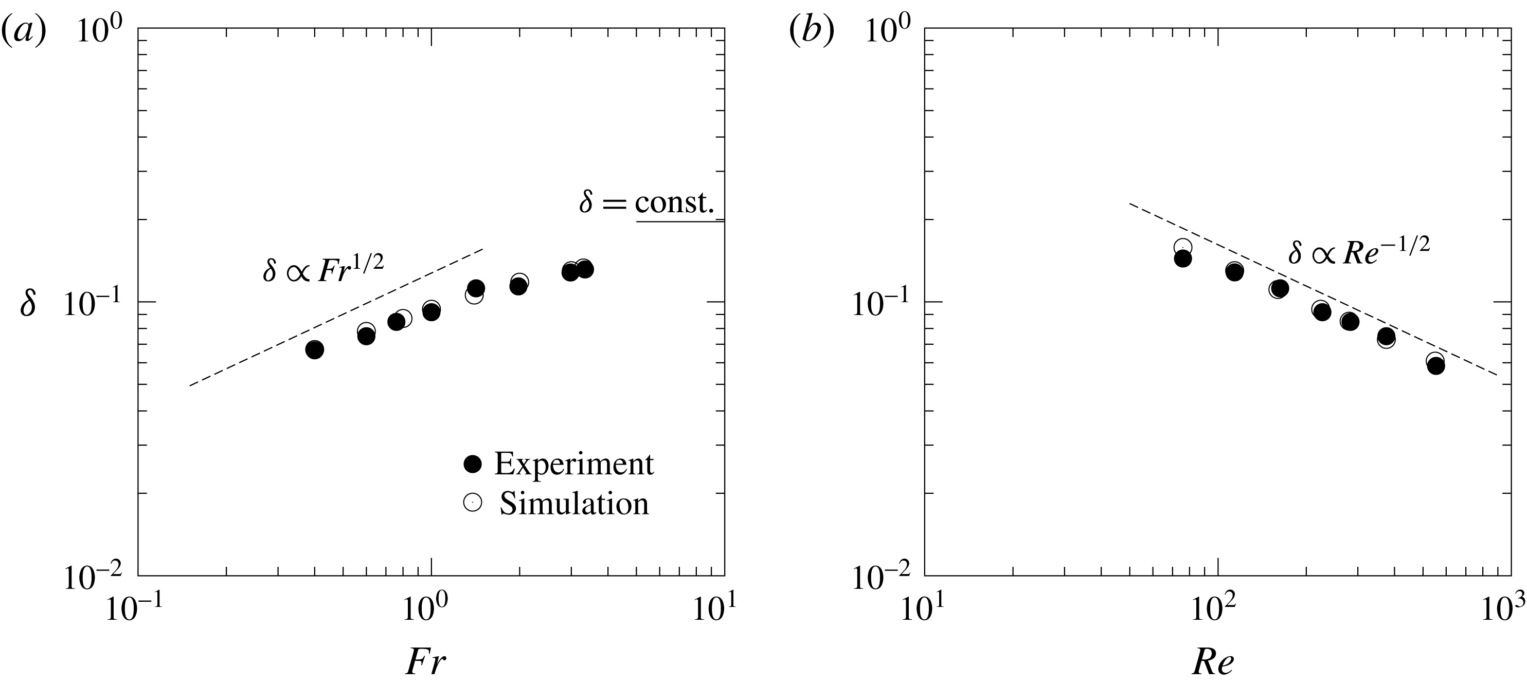
Boundary-layer thickness at the equator of the sphere (
 $y=z=0$
,
 $x=-0.5$
). (a) Froude number dependence at
 $Re\sim 220$
, obtained from PIV (A4–H4) and numerical simulations (a4–h4). (b) Reynolds number dependence at
 $Fr\sim 1$
, obtained from PIV (D1–D7) and numerical simulations (d1–d7). Dashed lines show the estimation given by (3.11), which is proportional to
 $Fr^{1/2}$
(
 $Fr\lesssim 1$
) for a constant
 $Re$
(a) and proportional to
 $Re^{-1/2}$
for a constant
 $Fr$
(b). The experimental result for an unstratified flow (
 $Fr=\infty$
) is shown in (a) by the line of
 $\unicode[STIX]{x1D6FF}=\text{const.}$

Since the jet originates from the velocity boundary layer on the sphere surface, it would be important to examine the approximate equality between the boundary-layer thickness and the jet radius. For this purpose, we next consider the velocity distribution in the boundary layer. Figure 12 shows the distribution of vertical velocity near the equator of the sphere (i.e. on the
 $x$
axis but outside the sphere (
 $x\leqslant -0.5$
)). This region has been selected since the boundary-layer thickness would be most clearly observed. The vertical velocity in the laboratory frame, i.e.
 $w-1$
, should be
 $-1$
on the sphere surface and it should approach zero far from the sphere. Since the spatial resolution of the lens with long focal length (
 $=$
105 mm) is
 $8\times 10^{-3}$
as noted in § 1, approximately ten data points exist in the boundary layer, whose thickness
 $\unicode[STIX]{x1D6FF}$
is estimated by the distance of the point of maximum vertical velocity from the surface of the sphere. In figure 12(a) the distance of the velocity peak from the sphere surface increases monotonically with
 $Fr$
, while the peak velocity decreases with
 $Fr$
. This shows that the boundary-layer thickness increases with the Froude number, consistent with the broader and slower jet observed at larger Froude numbers (figure 10
a). The numerical simulations and the experiments show good agreement. Figure 12(b) shows the Reynolds number dependence, and we find that the position of the velocity peak moves nearer to the sphere surface and the peak velocity increases as the Reynolds number increases. These effects of the Reynolds number on the velocity boundary layer are similar to those for a homogeneous fluid.
Finally in figure 13, we show the thickness of the velocity boundary layer
 $\unicode[STIX]{x1D6FF}$
, which is non-dimensionalised by
 $2a^{\ast }$
. In figure 13(a), the boundary-layer thickness increases with the Froude number in agreement with figure 12(a), while in figure 13(b), the thickness decreases with the Reynolds number corresponding to figure 12(b). If we expect that the boundary layer deforms into the jet, the thickness of the boundary layer should be approximately equal to the jet radius. We can confirm this (
 $\unicode[STIX]{x1D6FF}\sim T$
) by comparing figures 11 and 13, and the estimation
 $$\begin{eqnarray}\unicode[STIX]{x1D6FF}\sim T\sim \frac{l_{\unicode[STIX]{x1D708}}^{\ast }}{2a^{\ast }}=\left(\frac{Fr}{2Re}\right)^{1/2}\quad (Fr\lesssim 1)\end{eqnarray}$$
can be assured. This estimation gives two relations
 $$\begin{eqnarray}\unicode[STIX]{x1D6FF}\propto Fr^{1/2}\end{eqnarray}$$
for a constant
 $Re$
, and
 $$\begin{eqnarray}\unicode[STIX]{x1D6FF}\propto Re^{-1/2}\end{eqnarray}$$
for a constant
 $Fr$
, under the condition of sufficiently small
 $Fr({\lesssim}1)$
. Similarly to figure 11, the former relation (3.12) is observed in figure 13(a), and the latter relation (3.13) in figure 13(b), with good agreements between experiments and numerical simulations. Considering again that the thickness of the velocity boundary layer should asymptote to the value
 $\unicode[STIX]{x1D6FF}\sim \sqrt{1/Re}$
in a homogeneous fluid (
 $Fr\rightarrow \infty$
), we expect that the proportionality holds only for low
 $Fr({\lesssim}1)$
in figure 13(a), and
 $\unicode[STIX]{x1D6FF}$
should approach a constant value at large
 $Fr(\gg 1)$
. The experimentally observed boundary-layer thickness in an unstratified flow (
 $Fr=\infty$
) is also presented in figure 13(a), and
 $\unicode[STIX]{x1D6FF}$
asymptotes to that unstratified value as
 $Fr$
increases.
In a previous numerical simulation, Yick et al. (Reference Yick, Torres, Peacock and Stocker2009) considered that the spherical shell dragged by the sphere is the origin of the added drag, and the shell thickness is proportional to
 $\sqrt{\unicode[STIX]{x1D708}^{\ast }/N^{\ast }}=(Fr/Re)^{1/2}$
(cf. their figure 12b). In their paper the shell was defined by the region of large density perturbation from its background value (
 $\unicode[STIX]{x0394}\unicode[STIX]{x1D70C}>5\,\%$
), i.e. it was defined by the density difference rather than the velocity difference usually used for the definition of the velocity boundary layer. Then, the agreement with our result for the velocity boundary layer (3.11) may seem only accidental. However, since the density boundary-layer thickness is estimated by
 $\sqrt{\unicode[STIX]{x1D705}^{\ast }/N^{\ast }}=(Fr/(2Re\,Sc))^{1/2}$
(Hanazaki et al.
Reference Hanazaki, Nakamura and Yoshikawa2015), the proportionality to
 $(Fr/Re)^{1/2}$
should be observed also for the density boundary layer at a fixed Schmidt number. Therefore, the proportionality of the shell thickness to
 $(Fr/Re)^{1/2}$
would be consistent with our results.
4 Conclusions
We have observed the velocity around a sphere descending at a constant speed in a salt-stratified fluid, with particular attention to its dependence on the Froude number and the Reynolds number. The velocity distributions measured by PIV clarified many aspects of the predictions by numerical simulations and by the linear theory of internal waves which have not been identified experimentally.
The length of a jet, or similarly the height at which the vertical velocity becomes maximum, is determined by the vertical wavelength of the internal wave
 $\unicode[STIX]{x03C0}W^{\ast }/N^{\ast }$
(or
 $\unicode[STIX]{x03C0}Fr/2$
when non-dimensionalised by the sphere diameter
 $2a^{\ast }$
) which is predicted by linear wave theory. Then, the dimensional length of the jet would be determined by the stratification and the vertical velocity of the obstacle and not by the obstacle size.
The measured velocity distributions around the sphere generally agree with the numerical simulation and the thickness of the velocity boundary layer
 $\unicode[STIX]{x1D6FF}$
is proportional to
 $Fr^{1/2}$
and
 $Re^{-1/2}$
at low Froude numbers (
 $Fr\lesssim 1$
). This is in agreement with the simple dimensional analysis which predicts
 $\unicode[STIX]{x1D6FF}\sim l_{\unicode[STIX]{x1D708}}^{\ast }/2a^{\ast }=(Fr/2Re)^{1/2}$
, with
 $l_{\unicode[STIX]{x1D708}}^{\ast }=\sqrt{\unicode[STIX]{x1D708}^{\ast }/N^{\ast }}$
being the primitive length scale which has sometimes been used in stratified turbulence.
Since the vertical jet would be the continuation of the boundary layer on the sphere surface through the upper stagnation point of the sphere, the jet radius
 $T$
would be approximately equal to
 $\unicode[STIX]{x1D6FF}$
. The measured value of
 $T$
indeed agrees well with
 $\unicode[STIX]{x1D6FF}$
and
 $T$
is proportional to
 $Fr^{1/2}$
and
 $Re^{-1/2}$
at low Froude numbers (
 $Fr\lesssim 1$
), again in agreement with the dimensional analysis which predicts
 $T\sim \unicode[STIX]{x1D6FF}\sim l_{\unicode[STIX]{x1D708}}^{\ast }/2a^{\ast }=(Fr/2Re)^{1/2}$
.
Acknowledgements
This study was supported by JSPS KAKENHI grant nos 24656124, 15K17972.