2.1 Position–velocity space

We introduce a filtered phase-space distribution function $\bar{f}$ through the convolution

(2.1) $$\begin{eqnarray}\bar{f}(x,v,t)=\unicode[STIX]{x1D6F7}\ast f\equiv \int _{-\infty }^{\infty }\,\text{d}v^{\prime }\unicode[STIX]{x1D6F7}(v-v^{\prime })f(x,v^{\prime },t)\end{eqnarray}$$

using the filter function

(2.2) $$\begin{eqnarray}\unicode[STIX]{x1D6F7}(v)=\frac{1}{v_{0}\sqrt{2\unicode[STIX]{x03C0}}}\exp \left(-\frac{1}{2}\left(\frac{v}{v_{0}}\right)^{2}\right)\end{eqnarray}$$

in which $v_{0}$ is a parameter of choice and $f(x,v,t)$ is a solution of the Vlasov–Maxwell system

(2.3) $$\begin{eqnarray}\left.\begin{array}{@{}c@{}}{\displaystyle \frac{\unicode[STIX]{x2202}f}{\unicode[STIX]{x2202}t}}+v{\displaystyle \frac{\unicode[STIX]{x2202}f}{\unicode[STIX]{x2202}x}}-E(x,t){\displaystyle \frac{\unicode[STIX]{x2202}f}{\unicode[STIX]{x2202}v}}=0\\ {\displaystyle \frac{\unicode[STIX]{x2202}E}{\unicode[STIX]{x2202}x}}=1-\displaystyle \int _{-\infty }^{\infty }\,\text{d}vf(x,v,t)\end{array}\right\}\end{eqnarray}$$

incorporating a stationary background ion distribution. Application of the convolution defined in (2.1) to this entire system results in the filtered Vlasov–Poisson system

(2.4) $$\begin{eqnarray}\left.\begin{array}{@{}c@{}}{\displaystyle \frac{\unicode[STIX]{x2202}\bar{f}}{\unicode[STIX]{x2202}t}}+v{\displaystyle \frac{\unicode[STIX]{x2202}\bar{f}}{\unicode[STIX]{x2202}x}}-E(x,t){\displaystyle \frac{\unicode[STIX]{x2202}\bar{f}}{\unicode[STIX]{x2202}v}}=-v_{0}^{2}{\displaystyle \frac{\unicode[STIX]{x2202}^{2}\bar{f}}{\unicode[STIX]{x2202}x\unicode[STIX]{x2202}v}}\\ {\displaystyle \frac{\unicode[STIX]{x2202}E}{\unicode[STIX]{x2202}x}}=1-\displaystyle \int _{-\infty }^{\infty }\,\text{d}v\bar{f}(x,v,t).\end{array}\right\}\end{eqnarray}$$

The Vlasov–Poisson system is abandoned and replaced by the filtered Vlasov–Poisson system, which governs the evolution of $\bar{f}(x,v,t)$ while maintaining the relationship (2.1). The evolution of $f(x,v,t)$ is unaffected while the resolution in velocity contained in $\bar{f}(x,v,t)$ is limited by the choice of $v_{0}$ . Since $v_{0}$ is a parameter of choice, the resolution in velocity that is sought in any application is also a matter of choice. The filtered Vlasov equation can be thought of as an equation governing the evolution of an observed distribution, observed with an idealized detector with perfect Gaussian response. The act of observing the Vlasov distribution does not affect its evolution. The method introduces no intrinsic error into the evolution of the Vlasov–Poisson system.

The density and flux moments are invariant under filtering; i.e.

(2.5) $$\begin{eqnarray}\int _{-\infty }^{\infty }\,\text{d}v\bar{f}(x,v,t)=\int _{-\infty }^{\infty }\,\text{d}vf(x,v,t)\end{eqnarray}$$

and

(2.6) $$\begin{eqnarray}\int _{-\infty }^{\infty }\,\text{d}vv\bar{f}(x,v,t)=\int _{-\infty }^{\infty }\,\text{d}vvf(x,v,t).\end{eqnarray}$$

Thus, at any instant the charge and current distributions are unaltered and, consequently, the evolution of the electromagnetic field remains unchanged. Finally, with an appropriate choice of $v_{0}$ filamentation is prevented from evolving down to the discretized velocity grid while information that might normally be hidden below the filamentation can be revealed (Klimas et al. Reference Klimas, Vinas and Araneda2017).

To our knowledge, a systematic study of the regularity of the filtered Vlasov–Poisson system solutions has not been done at this time. However, Klimas (Reference Klimas1987) has shown that the first derivative with respect to velocity of the filtered Vlasov–Poisson solutions can be uniformly bounded from above. This is a direct consequence of the convolution filter (2.1) and filter choice (2.2). Further, Klimas & Fitzenreiter (Reference Klimas and Fitzenreiter1988) have shown that the velocity dependence of the filtered distribution can be analytically continued off the real axis to find that the distribution is entire on the complex velocity plane as long as the zeroth and first moments of the distribution on the real axis are bounded.

The filtered Vlasov–Poisson system (2.4) is the basis for the flux-balance simulation code. For all flux-balance simulation results discussed below, periodic simulations are carried out on a spatial interval $(-L_{k}\leqslant x\leqslant L_{k})$ . Time is measured in units of $\unicode[STIX]{x1D714}_{pe}^{-1}$ with $\unicode[STIX]{x1D714}_{pe}$ the electron plasma frequency, length is measured in units of $L_{k}$ , speed is measured in units of $v_{th}(L_{k}/\unicode[STIX]{x1D706}_{D})$ in which $v_{th}$ is the thermal speed and $\unicode[STIX]{x1D706}_{D}=(v_{th}/\unicode[STIX]{x1D714}_{pe})$ is the Debye length. With these choices, the dimensionless distribution function $\bar{f}$ is measured in units of $(L_{k}^{2}\unicode[STIX]{x1D714}_{pe})^{-1}$ and the dimensionless electric field is measured in units of $4\unicode[STIX]{x03C0}n_{0}L_{k}$ , in which $n_{0}$ is the density of the stationary background ion distribution; the dimensionless density of the background ion distribution is 1.

2.2 Fourier–Fourier transformed space

It has been shown that the filtered Vlasov–Poisson system (2.4) can be efficiently integrated numerically in a transformed space (Klimas & Farrell Reference Klimas and Farrell1994). With this approach, the entire system (2.4) is Fourier transformed with respect to both position, $x$ , and velocity, $v$ , and in addition the splitting scheme due to Cheng & Knorr (Reference Cheng and Knorr1976) is employed.

Early attempts to solve the filamentation problem in a discretized ( $x,v$ ) phase space using the filtered Vlasov–Poisson approach found that the filtered system is numerically unstable. In fact, Figua et al. (Reference Figua, Bouchut, Feix and Fijalkow2000) later argued that the filtered Vlasov–Poisson system is unconditionally unstable in the discretized ( $x,v$ ) phase space. This was the motivation for turning to the Fourier–Fourier transformed system, which was found stable, flexible and fast. Although no longer true (Vinas & Klimas Reference Vinas and Klimas2018), the choice of doubly Fourier transformed solutions was a matter of necessity at the time. Now, with the recurrence problem solution that we present in this paper, these solutions are of further interest.

It should be remembered that the Vlasov equation provides the evolution of the one-body probability distribution. The Vlasov equation is the result of an ensemble average in which all spatial dependence below the Debye length has been relegated to two-body and higher-order distributions whose effects are then neglected (Krall & Trivelpiece Reference Krall, Trivelpiece and Harnwell1986). We take the position that any solution of the Vlasov–Poisson system that exhibits spatial dependence below the Debye length invalidates the foundation of the Vlasov equation itself and must be rejected. Thus, we use a truncated discrete Fourier series expansion of the spatial dependence under the assumption that the expansion will be sufficient to resolve the larger spatial scales of a valid Vlasov distribution.

Using the Fourier transformation definitions

(2.7) $$\begin{eqnarray}\bar{K}_{m}(\unicode[STIX]{x1D707},t)=\frac{1}{2}\int _{-1}^{1}\,\text{d}x\text{e}^{-\text{i}m\unicode[STIX]{x03C0}x}\int _{-\infty }^{\infty }\,\text{d}v\text{e}^{\text{i}\unicode[STIX]{x03C0}\unicode[STIX]{x1D707}v}\bar{f}(x,v,t)\end{eqnarray}$$

and

(2.8) $$\begin{eqnarray}\bar{f}(x,v,t)=\mathop{\sum }_{m=-\infty }^{\infty }\text{e}^{\text{i}m\unicode[STIX]{x03C0}x}\frac{1}{2}\int _{-\infty }^{\infty }\,\text{d}\unicode[STIX]{x1D707}\text{e}^{-\text{i}\unicode[STIX]{x03C0}\unicode[STIX]{x1D707}v}\bar{K}_{m}(\unicode[STIX]{x1D707},t)\end{eqnarray}$$

with the electric field given by

(2.9) $$\begin{eqnarray}E(x,t)=\mathop{\sum }_{m=-\infty }^{\infty }\text{e}^{\text{i}m\unicode[STIX]{x03C0}x}E_{m}(t)\end{eqnarray}$$

the filtered Vlasov–Poisson system (2.4) can be doubly Fourier transformed to obtain

(2.10) $$\begin{eqnarray}\frac{\unicode[STIX]{x2202}\bar{K}_{m}}{\unicode[STIX]{x2202}t}+m\frac{\unicode[STIX]{x2202}\bar{K}_{m}}{\unicode[STIX]{x2202}\unicode[STIX]{x1D707}}+\text{i}\unicode[STIX]{x03C0}\unicode[STIX]{x1D707}\mathop{\sum }_{n=-\infty }^{\infty }E_{m-n}\bar{K}_{n}=\unicode[STIX]{x1D700}m\unicode[STIX]{x1D707}\bar{K}_{m}\end{eqnarray}$$

in which

(2.11) $$\begin{eqnarray}\unicode[STIX]{x1D700}=(\unicode[STIX]{x03C0}v_{0})^{2}\equiv \frac{1}{\unicode[STIX]{x1D707}_{0}^{2}}\end{eqnarray}$$

and the electric field Fourier components are given by

(2.12) $$\begin{eqnarray}\text{i}\unicode[STIX]{x03C0}E_{m-n}(t)=\left\{\begin{array}{@{}ll@{}}{\displaystyle \frac{\bar{K}_{m-n}(\unicode[STIX]{x1D707}=0,t)}{m-n}}\quad & m\neq n\\ 0\quad & m=n.\end{array}\right.\end{eqnarray}$$

In the doubly Fourier transformed space

(2.13) $$\begin{eqnarray}\bar{K}_{m}(\unicode[STIX]{x1D707},t)=\unicode[STIX]{x1D6F7}(\unicode[STIX]{x1D707})K_{m}(\unicode[STIX]{x1D707},t)\end{eqnarray}$$

in which $K_{m}(\unicode[STIX]{x1D707},t)$ is the Fourier transform defined by (2.7) of the unfiltered $f(x,v,t)$ and the Fourier transformed filter function is given by

(2.14) $$\begin{eqnarray}\unicode[STIX]{x1D6F7}(\unicode[STIX]{x1D707})=\exp \left(-\frac{1}{2}\left(\frac{\unicode[STIX]{x1D707}}{\unicode[STIX]{x1D707}_{0}}\right)^{2}\right).\end{eqnarray}$$

The analogue to the $x$ -shift in the Cheng and Knorr splitting scheme is

(2.15) $$\begin{eqnarray}\frac{\unicode[STIX]{x2202}\bar{K}_{m}}{\unicode[STIX]{x2202}t}+m\frac{\unicode[STIX]{x2202}\bar{K}_{m}}{\unicode[STIX]{x2202}\unicode[STIX]{x1D707}}=\unicode[STIX]{x1D700}m\unicode[STIX]{x1D707}\bar{K}_{m}.\end{eqnarray}$$

Updating forward by one time step $\unicode[STIX]{x0394}t$ yields

(2.16) $$\begin{eqnarray}\bar{K}_{m}(\unicode[STIX]{x1D707},t_{n}+\unicode[STIX]{x0394}t)=\bar{K}_{m}(\unicode[STIX]{x1D707}-m\unicode[STIX]{x0394}t,t_{n})\exp \left[\unicode[STIX]{x1D700}\left(\unicode[STIX]{x1D707}m\unicode[STIX]{x0394}t-{\textstyle \frac{1}{2}}\left(m\unicode[STIX]{x0394}t\right)^{2}\right)\right]\!.\end{eqnarray}$$

Notice the important feature: if, in a numerical application $\unicode[STIX]{x1D707}$ appears on a discrete grid $\unicode[STIX]{x1D707}_{j}=j\unicode[STIX]{x0394}\unicode[STIX]{x1D707}\;(j=0,1,2,\ldots )$ , then no interpolation is necessary if $\unicode[STIX]{x0394}\unicode[STIX]{x1D707}=\unicode[STIX]{x0394}t$ . Data are simply moved from one grid point to another while being modified by the exponential factor in (2.16). The Cheng and Knorr $v$ -shift is

(2.17) $$\begin{eqnarray}\frac{\unicode[STIX]{x2202}\bar{K}_{m}}{\unicode[STIX]{x2202}t}=-\text{i}\unicode[STIX]{x03C0}\unicode[STIX]{x1D707}\mathop{\sum }_{n=-\infty }^{\infty }E_{m-n}\bar{K}_{n},\end{eqnarray}$$

which can be backward Fourier transformed in the $x$ -variable to obtain

(2.18) $$\begin{eqnarray}\frac{\unicode[STIX]{x2202}\bar{K}(x,\unicode[STIX]{x1D707},t)}{\unicode[STIX]{x2202}t}=-\text{i}\unicode[STIX]{x03C0}\unicode[STIX]{x1D707}E(x,t)\bar{K}(x,\unicode[STIX]{x1D707},t)\end{eqnarray}$$

or

(2.19) $$\begin{eqnarray}\bar{K}(x,\unicode[STIX]{x1D707},t_{n}+\unicode[STIX]{x0394}t)=\bar{K}(x,\unicode[STIX]{x1D707},t_{n})\exp [-\text{i}\unicode[STIX]{x03C0}\unicode[STIX]{x1D707}E(x,t_{n})\unicode[STIX]{x0394}t]\end{eqnarray}$$

since the electric field is held fixed during the $v$ -shift. This result is then Fourier transformed back to the doubly transformed space; fast Fourier transforms (FFTs) are used for the transformations. Again, no interpolation is necessary.

The overall marching scheme is quite fast; the lack of interpolation plus the use of FFTs contribute. Usually, $\unicode[STIX]{x0394}\unicode[STIX]{x1D707}=\unicode[STIX]{x0394}t=0.1$ is sufficient. Simulations are carried out on a $(m,\unicode[STIX]{x1D707})$ grid with $-m_{\max }\leqslant m\leqslant m_{\max }$ and $0\leqslant \unicode[STIX]{x1D707}\leqslant \unicode[STIX]{x1D707}_{\max }$ . For weak Landau damping simulations, $m_{\max }$ can be quite small since, often, very few spatial modes besides the fundamental mode are excited.

3.1 Flux-balance simulation, freestreaming

With the coupling between electrons and electric field disabled in the flux-balance code by setting $E(x,t)=0$ in (2.4), a freestreaming simulation results. Due to the lack of mode–mode coupling in such a simulation, only the three spatial Fourier modes $m=0,\pm 1$ contained in the initial state (3.1) are found in the simulated phase-space distribution at any later time. The perturbation on the thermal background is at wavelength $\unicode[STIX]{x1D706}_{\pm 1}=2$ . Thus, from (1.1) we expect the first recurrence of this wavelength at $t_{\text{rec}}(m=1)=180$ .

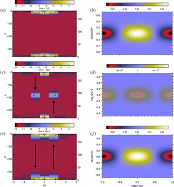
Figure 1 provides a comparison of the ‘standard’ representation of the phase-space distribution in $(x,v)$ with its Fourier transformed ‘spectral’ representation in $(m,\unicode[STIX]{x1D707})$ at three times, $t=0$ , $t=t_{\text{rec}}(1)/2$ , and $t=t_{\text{rec}}(1)$ . The space-averaged component of the distribution has been removed from the standard representation in the figure but not from the spectral representation. Filamentation filtration has been enabled with filter half-width $v_{0}=2\unicode[STIX]{x0394}v=0.0222$ and, therefore from (2.11), $\unicode[STIX]{x1D707}_{0}\simeq 14.3$ . The intensities of the spectral representations are plotted as $\log _{10}(\text{abs}(\text{FFT}(\,\bar{f})))$ with any point falling under the minimum, $-14$ , being replaced by the minimum.

Figure 1.

At $t=0$ (a,b), half the mode-1 recurrence time, $t=90$ (c,d), and at the recurrence time, $t=180$ (e,f). (b,d,f) Standard ( $x,v$ ) representation of filtered phase-space distribution with space-averaged component removed. (a,c,e) Fourier transformed spectral representation of filtered phase-space distribution. Red stars show positions of peak values in the individual modes.

At $t=0$ (a,b), the spatial $\cos \unicode[STIX]{x03C0}x$ perturbation introduced by the initial state (3.1) is evident in the standard phase-space representation to the right. The thermal velocity distributions of the three $m=0,\pm 1$ modes are transformed into the Gaussian distributions centred at $\unicode[STIX]{x1D707}=0$ shown in the spectral phase-space representation to the left. In this representation, the modes are periodic in $\unicode[STIX]{x1D707}$ and therefore the intensities of the modes for negative $\unicode[STIX]{x1D707}$ -values appear at the top of the panel. (Each of the panels in this figure showing a spectral distribution shows the distribution at both positive and negative $\unicode[STIX]{x1D707}$ -values in this manner.)

At $t=t_{\text{rec}}(1)/2$ (c,d), in agreement with (2.16) the centroids of the $m=0,\pm 1$ modes in the spectral space have propagated to $\unicode[STIX]{x1D707}(t)=\unicode[STIX]{x1D707}(t=0)+mt$ , leaving the $m=0$ mode unmoved and the $m=\pm 1$ modes at the midpoint of the $\unicode[STIX]{x1D707}$ grid. In the spectral space, the filtered phase-space distribution $\bar{K}_{m}$ is obtained through a simple multiplication of the unfiltered distribution $K_{m}$ by the Fourier transformed filamentation filter, which is a Gaussian centred at $\unicode[STIX]{x1D707}=0$ with, in this case, half-width $\unicode[STIX]{x1D707}_{0}\simeq 14.3$ . At this time, the centroids of the $m=\pm 1$ modes are at approximately 6 filter half-widths away from the peak in the filter and are consequently greatly reduced in amplitude. The standard phase-space representation, shown on the right, is dominated at this time by filamentation but it is, similarly, greatly reduced in amplitude.

At $t=t_{\text{rec}}(1)$ (e,f), the centroids of the $m=\pm 1$ modes have moved in the $\unicode[STIX]{x1D707}$ -variable to exactly one period away from their initial positions. Due to the periodicity of the spectral phase-space distribution, the initial distribution is reproduced at this time in both the spectral and the standard representations. In this freestreaming example recurrence is due to the periodicity in $\unicode[STIX]{x1D707}$ of the individual spatial Fourier modes combined with their propagation in $\unicode[STIX]{x1D707}$ according to $\unicode[STIX]{x1D707}(t)=\unicode[STIX]{x1D707}(t=0)+mt$ .

It is important to note that in the spectral space the transformed filamentation filter is also periodic in $\unicode[STIX]{x1D707}$ . In addition to the Gaussian centred at $\unicode[STIX]{x1D707}=0$ , the filter has Gaussian peaks at $\unicode[STIX]{x1D707}=\pm t_{\text{rec}}(1)=\pm 180$ as well. Minima in filter strength are at $\unicode[STIX]{x1D707}=\pm t_{\text{rec}}(1)/2$ . As the centroids of the $m=\pm 1$ modes start to move away from their initial positions, the filamentation that they carry is reduced in amplitude due to the decreasing amplitude of the local filamentation filter. Once the modes propagate past the minima, however, the filamentation begins to increase and eventually coalesce back to the initial state. The periodicity of the filter allows this reversal of the filtering process at $t=t_{\text{rec}}(1)/2$ and the consequent reformation of the initial state. This is the manifestation of recurrence in this Fourier–Fourier transformed space.

3.2 Flux-balance simulation, Landau damping

With the coupling between electrons and electric field replaced in the flux-balance code – i.e. with $E(x,t)\neq 0$ in (2.4) – a Landau damping simulation follows from the initial state (3.1). Here we use the same simulation set-up as in the preceding section, with one exception. For clarity in the figures, the filamentation filter has been disabled. This choice does not affect the conclusions that are drawn. A weak initial perturbation and a coarse velocity grid spacing have been chosen to enhance the recurrence effects in the simulation. In this section we compare the recurrence effects seen in the electric field evolution with those seen in the spectral representation of the phase-space distribution.

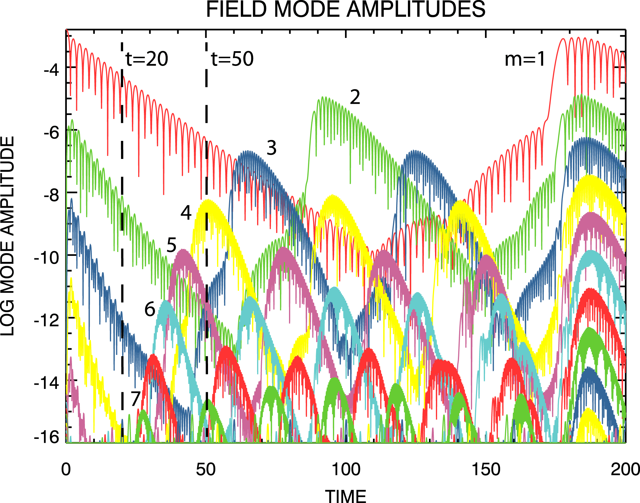
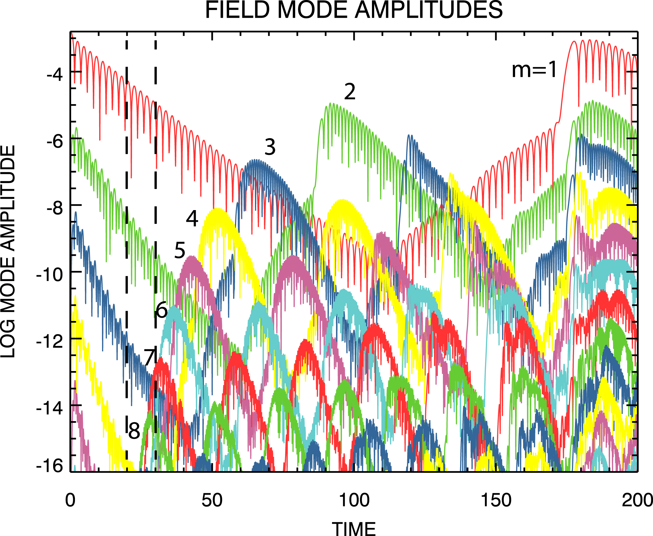
Figure 2 shows the evolution with time of the dominant field mode amplitudes for the unfiltered Landau damping simulation. The curve labelled $m=1$ corresponds to the longest wavelength in the field, $\unicode[STIX]{x1D706}_{1}=2$ ( $2L_{k}$ ); the wavelengths of higher-order modes follow from $\unicode[STIX]{x1D706}_{m}=\unicode[STIX]{x1D706}_{1}/m$ . The bursts that can be seen in the field mode amplitudes are due to the recurrence effect, which occurs at approximately $t_{\text{rec}}(m)$ given by (1.1). Only the first recurrence of the $\unicode[STIX]{x1D706}_{1}$ mode is shown but higher-order modes exhibit multiple recurrences at $n=1,2,3,\ldots$ in (1.1).

Figure 2.

Time evolution of the longer wavelength electric field mode amplitudes for the unfiltered flux-balance Landau damping simulation. Amplitudes of shorter wavelength modes lie below the $10^{-16}$ cutoff of the figure. Labels refer to mode numbers. Vertical dashed lines are at $t=20$ and $t=50$ .

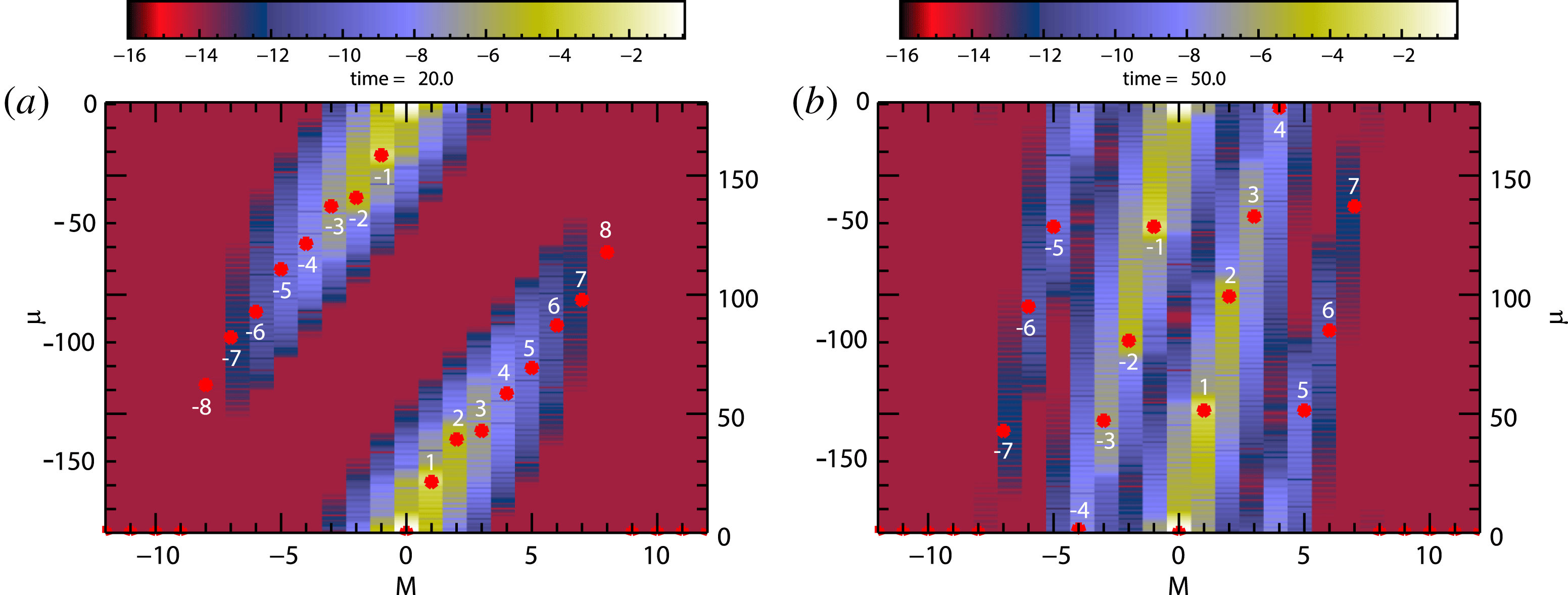
Figure 3 shows the spectral representation of the phase-space distribution for this simulation at $t=20$ (a) and $t=50$ (b). These times correspond to the dashed lines drawn at $t=20$ and $t=50$ on figure 2. It can be seen that at $t=20$ all of the $m\neq 0$ mode centroids have propagated away from their initial positions $\unicode[STIX]{x1D707}=0$ . Interestingly, the $m=\pm 1,2$ modes appear to be moving in approximate agreement with $\unicode[STIX]{x1D707}(t)=\unicode[STIX]{x1D707}(0)+mt$ but the rest are moving much slower than that relation would predict. None of the centroids have propagated an entire period in $\unicode[STIX]{x1D707}$ at this time. Notice, from figure 2, that there is also no evidence in the field of recurrence at this time. At $t=50$ , the centroids of modes $m=\pm (5{-}7)$ have progressed more than one period in $\unicode[STIX]{x1D707}$ and are on their way to a second period while those of modes $m=\pm (1{-}4)$ are still traversing their first period. Based on the positions of the peaks in the field mode magnitudes shown in figure 2, we can say that at $t=50$ wavelengths $m=1{-}3$ have not yet recurred and the $m=4$ wavelength is at recurrence. The $m=5$ wavelength has recently recurred and the $m=6$ and $m=7$ wavelengths have recurred earlier. All of these observations are in complete agreement with the positions of the mode centroids shown in the right panel at $t=50$ .

Figure 3.

Fourier transformed spectral representations of phase-space distribution at $t=20$ (a) and $t=50$ (b). Red stars show positions of peak values in the individual modes. Numbers indicate mode numbers.

We therefore conclude that in the Fourier transformed spectral space recurrence is exhibited as periodic traversals of the space in the $\unicode[STIX]{x1D707}$ -direction of the spatial Fourier modes contained in the phase-space distribution. A period in the $\unicode[STIX]{x1D707}$ -direction is given by $\unicode[STIX]{x1D707}=0-\unicode[STIX]{x1D707}=\pm \unicode[STIX]{x1D707}_{\text{rec}}$ in which $\unicode[STIX]{x1D707}_{\text{rec}}=2/\unicode[STIX]{x0394}v$ . Periodic behaviour in $\unicode[STIX]{x1D707}$ is due to the finite size of the $\unicode[STIX]{x1D707}$ -grid which is directly related to the finite resolution $\unicode[STIX]{x0394}v$ in velocity in the $(x.v)$ space.

4.1 Spectral boundary conditions

Spectral code simulations are carried out on a computational $(m,\unicode[STIX]{x1D707})$ -grid with $-m_{\max }\leqslant m\leqslant m_{\max }$ and $0\leqslant \unicode[STIX]{x1D707}\leqslant \unicode[STIX]{x1D707}_{\max }$ . Setting the maximum number of spatial Fourier modes is a matter of setting $m_{\max }$ sufficiently large to find that the simulation results are independent of $m_{\max }$ . The boundary conditions on the $\unicode[STIX]{x1D707}$ -boundaries are relatively simple but also central to the recurrence issue in the spectral code.

For this discussion of the $\unicode[STIX]{x1D707}$ -boundaries we will assume that $\unicode[STIX]{x0394}\unicode[STIX]{x1D707}=\unicode[STIX]{x0394}t$ (see (2.16) and related discussion). Then, for the $x$ -shift (2.16) a step forward in time involves a simple transfer of data from grid point to grid point. For $m>0$ the transfer is in the direction toward larger $\unicode[STIX]{x1D707}$ and for $m<0$ it is in the opposite direction. In either case, information approaching an outflow boundary ( $\unicode[STIX]{x1D707}=0$ for $m<0$ or $\unicode[STIX]{x1D707}=\unicode[STIX]{x1D707}_{\max }$ for $m>0$ ) is completely unaffected by the presence of the boundary. No boundary conditions at all are required at the outflow boundaries. However, buffers filled with appropriate data must be placed just outside the inflow boundaries. At $\unicode[STIX]{x1D707}=0$ for $m>0$ the relationship $\bar{K}_{m}(-\unicode[STIX]{x1D707},t)=\bar{K}_{-m}^{\ast }(\unicode[STIX]{x1D707},t)$ , which follows from the reality of $f$ and $\bar{f}$ , is used to fill the inflow buffer with data that are available just inside of the $(\unicode[STIX]{x1D707}=0,m<0)$ outflow boundary. In this way, outflowing data at $(\unicode[STIX]{x1D707}=0,m<0)$ are recycled to inflowing data at $(\unicode[STIX]{x1D707}=0,m>0)$ . Taken as a whole, the boundary at $\unicode[STIX]{x1D707}=0$ is a closed system; external boundary conditions are not imposed at $\unicode[STIX]{x1D707}=0$ . However, a buffer filled with inflow data is necessary just outside of the inflow boundary $(\unicode[STIX]{x1D707}=\unicode[STIX]{x1D707}_{\max },m<0)$ . This is, in fact, the only boundary condition that is imposed on the entire simulation domain. We will show that the presence or absence of recurrence in the spectral code can depend on the choice of data for this buffer.

4.2 Spectral simulation, recycled buffer input, recurrent, $\unicode[STIX]{x1D707}_{\max }=90$

We first choose buffer data for the $(\unicode[STIX]{x1D707}=\unicode[STIX]{x1D707}_{\max },m<0)$ inflow boundary to produce recurrence in the spectral code. Our goal here is to impose on the spectral code set-up the periodicity in $\unicode[STIX]{x1D707}$ exhibited by the doubly Fourier transformed flux-balance phase-space distribution discussed above in § 3. Initially, we will discuss unfiltered spectral code simulations.

Let $\unicode[STIX]{x1D707}_{\max }=\unicode[STIX]{x1D707}_{\text{rec}}/2=90$ and use the relationship $K_{-m}(\unicode[STIX]{x1D707}_{\max }+\unicode[STIX]{x1D6FF}\unicode[STIX]{x1D707},t)=K_{m}^{\ast }(\unicode[STIX]{x1D707}_{\max }-\unicode[STIX]{x1D6FF}\unicode[STIX]{x1D707},t)$ to fill the buffer at the inflowing boundary $(\unicode[STIX]{x1D707}=\unicode[STIX]{x1D707}_{\max },m<0)$ at each time step. 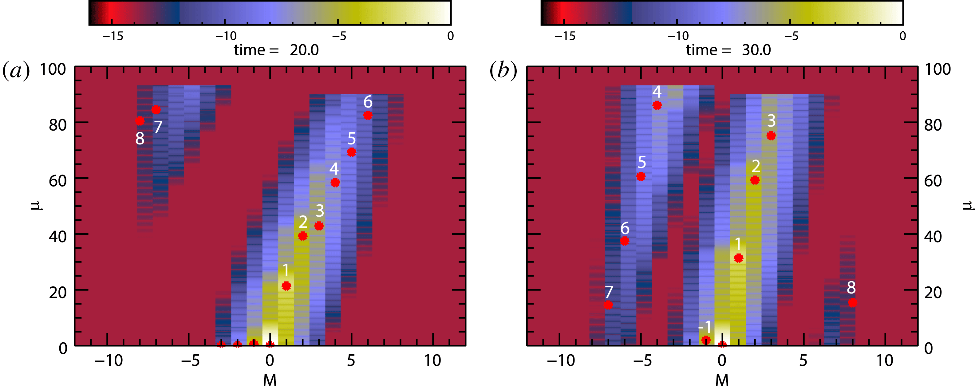Then, the periodic circulation in $\unicode[STIX]{x1D707}$ that leads to recurrence in the flux-balance code is imposed on the spectral code evolution. Figure 4 provides snapshots of the spectral phase-space distribution obtained in this manner. A comparison with figure 3 (the right panels are at different times) shows that the periodic circulation of the Fourier transformed flux-balance phase-space distribution shown there is reproduced by the spectral code in the $0\leqslant \unicode[STIX]{x1D707}\leqslant \unicode[STIX]{x1D707}_{\max }$ half of the full phase space. Since it is this periodicity that leads to recurrence, we expect this spectral Landau damping simulation to exhibit the same recurrence effects as the flux-balance simulation.

Figure 4.

Spectral representations of phase-space distribution at $t=20$ (a) and $t=30$ (b) taken directly from spectral code. Red stars show positions of peak values in the individual modes. Numbers indicate mode numbers.

Figure 5.

Time evolution of the electric field mode amplitudes from the unfiltered spectral Landau damping simulation using $\unicode[STIX]{x1D707}_{\max }=90$ and recirculating inflow boundary data. Labels refer to mode numbers. Vertical dashed lines are at $t=20$ and $t=30$ .

Figure 5 shows the evolution of the electric field mode magnitudes obtained from this spectral Landau damping simulation. A comparison with figure 2 shows a striking resemblance with the flux-balance results. The vertical dashed-lines are at $t=20$ (left) and $t=30$ (right). From the figure, at $t=20$ there is no sign of recurrence but at $t=30$ mode $m=8$ has already recurred and mode $m=7$ is about to. Although difficult to see, the positions of the mode amplitude peaks in figure 4 are in good agreement with the evolution shown in figure 5.

We conclude, therefore, that with particular $(\unicode[STIX]{x1D707}=\unicode[STIX]{x1D707}_{\max },m<0)$ inflow boundary data, spectral code simulations can exhibit the same recurrence effects shown by the $(x,v)$ -based flux-balance simulations.

4.3 Spectral simulation, recycled buffer input, non-recurrent, $\unicode[STIX]{x1D707}_{\max }=1900$

Figure 6.

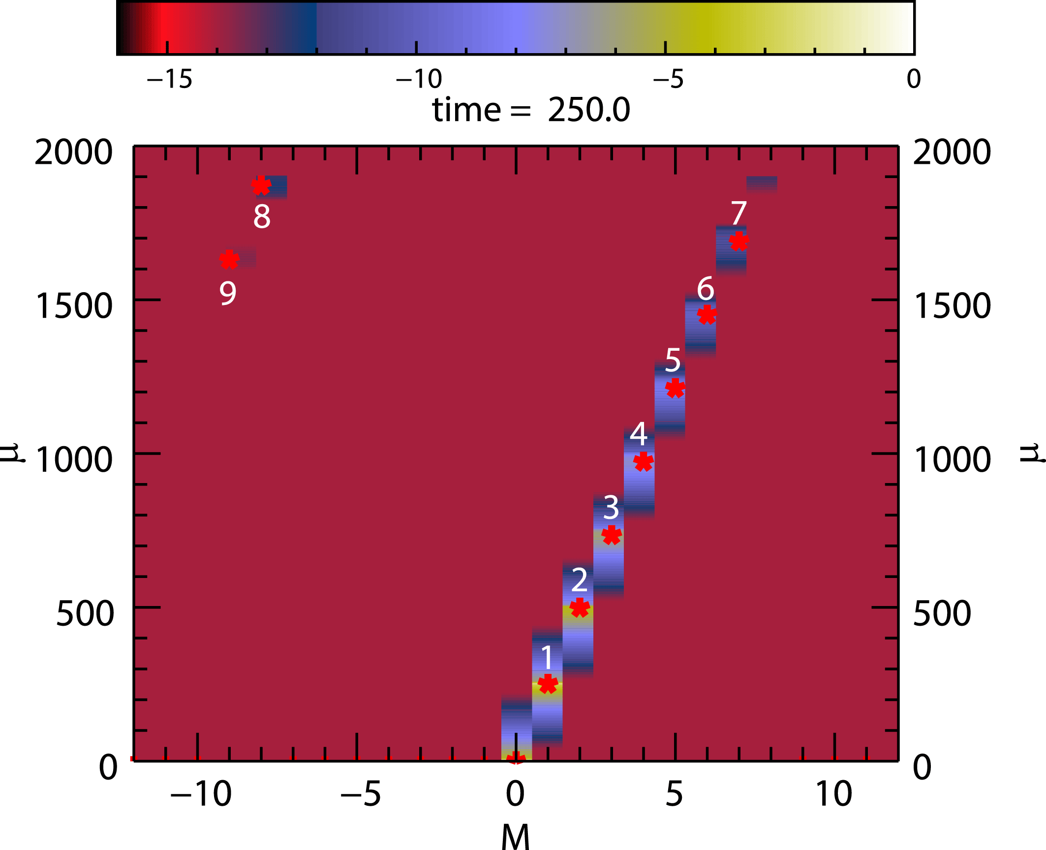
Spectral representation of phase-space distribution at $t=250$ taken directly from spectral code. Red stars show positions of peak values in the individual modes. Numbers indicate mode numbers.

In this section we continue with the spectral code, the same initial state (3.1), and the same recirculating inflow boundary data as in the preceding section, but we move the $\unicode[STIX]{x1D707}_{\max }$ boundary to the much larger value $\unicode[STIX]{x1D707}_{\max }=1900$ . For the $m=1$ mode we then expect $t_{\text{rec}}(1)\simeq 3800$ , the first recurrence time for the $m=8$ mode at $t_{\text{rec}}(8)\simeq 475$ , and the time for the $m=8$ mode to first reach $\unicode[STIX]{x1D707}_{\max }$ given by $t_{\max }(8)=t_{\text{rec}}(8)/2\simeq 237.5$ . Figure 6 shows the spectral phase-space distribution obtained at the end of this Landau damping simulation at $t=250$ . In agreement with this estimate of $t_{\max }(8)$ , we see that the $m=8$ mode peak has just been recycled from the positive to the negative side of the $m$ -distribution as a consequence of having reached the $\unicode[STIX]{x1D707}_{\max }$ -boundary.

Figure 7.

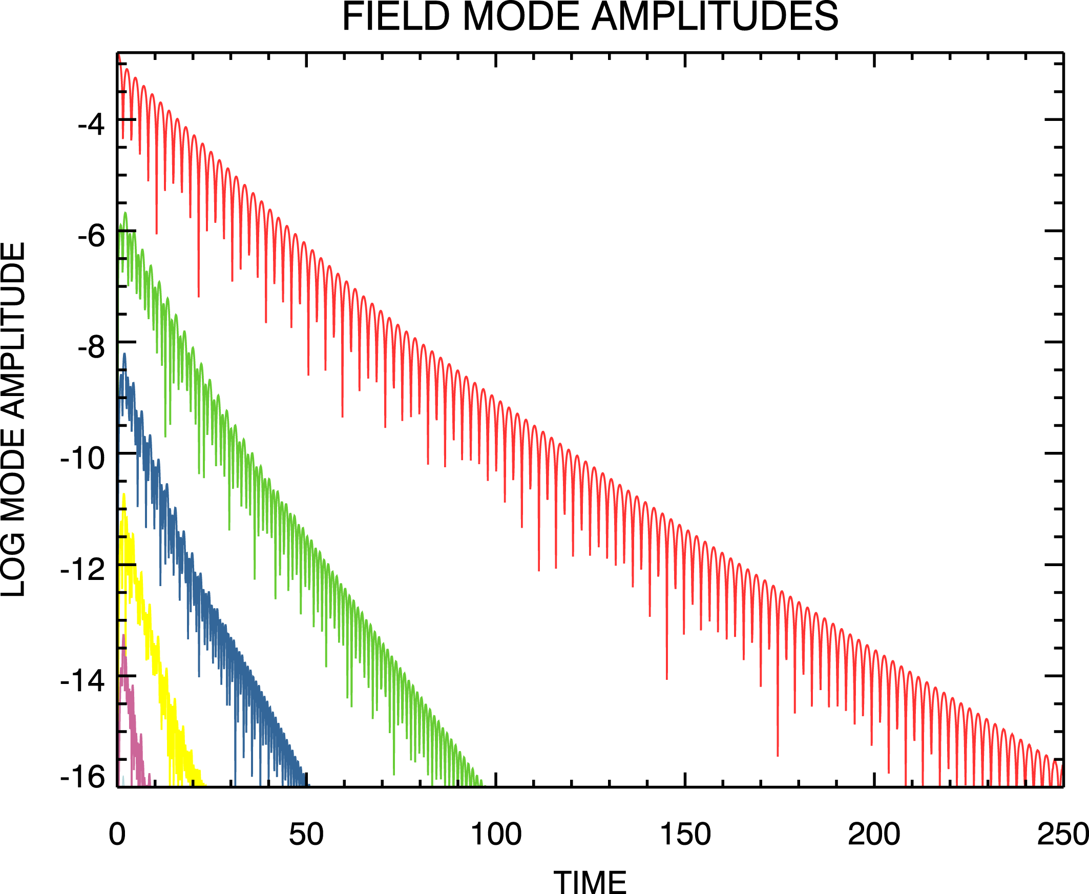
Time evolution of the electric field mode amplitudes from the unfiltered spectral Landau damping simulation using $\unicode[STIX]{x1D707}_{\max }=1900$ and recirculating inflow boundary data. Modes are ordered with decreasing amplitude with $m=1$ the dominant one.

Figure 7 shows the evolution in time of the field mode magnitudes that results as a consequence of moving the $\unicode[STIX]{x1D707}$ -boundary to $\unicode[STIX]{x1D707}_{\max }=1900$ . The recurrence effects shown in figure 5 for the case $\unicode[STIX]{x1D707}_{\max }=90$ have been removed. A straightforward persisting Landau damping simulation results.

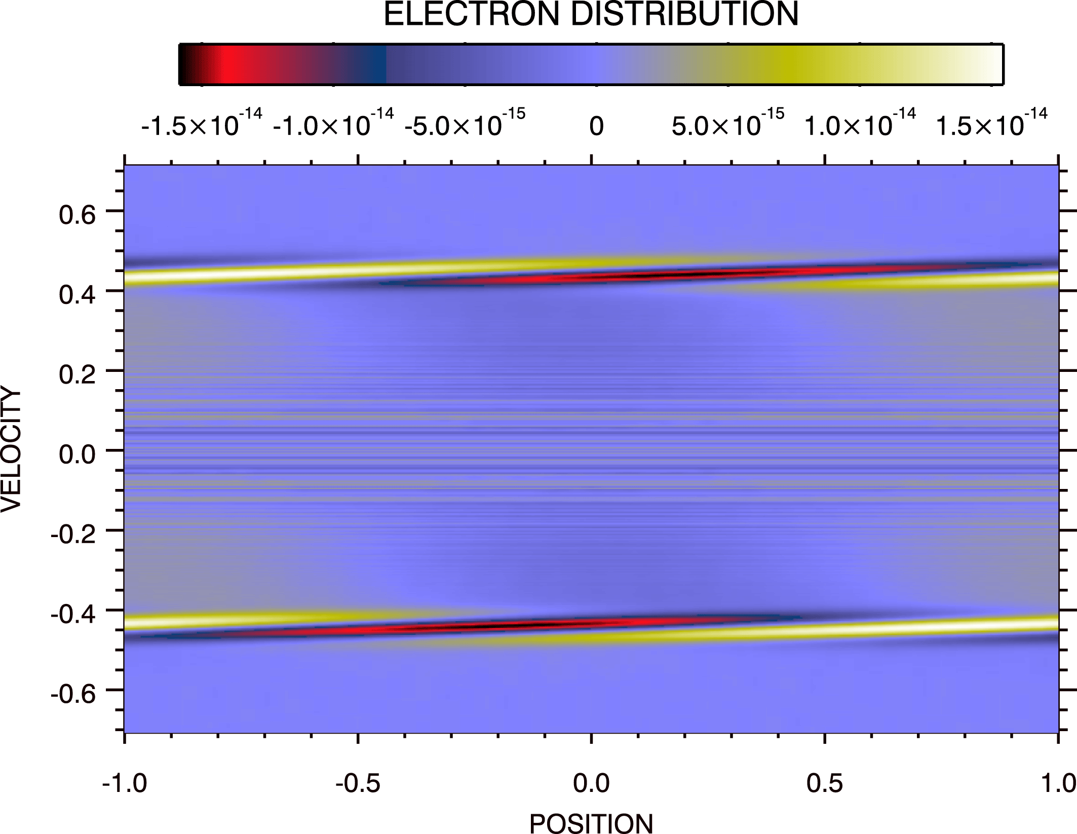
By the end of this Landau damping simulation at $t=250$ , the $(x,v)$ phase-space perturbation distribution is highly filamented (not shown). In the next section, we will use the results of this simulation as a standard to measure the accuracy of simulations in which recurrence has been removed. Those simulations will be filtered and will not exhibit filamentation at $t=250$ . The relationship between filtered and unfiltered phase-space distributions given by (2.1) applies. If we have been able to compute the unfiltered distribution $f(x,v,t)$ , then the filtered distribution $\bar{f}(x,v,t)$ can be obtained through (2.1). To enable comparison with the filtered results of the next section, we have applied (2.1) to the unfiltered $f(x,v,t=250)$ obtained from this simulation. The result is shown in figure 8. Notice, the magnitude of this perturbation between the disturbances at the resonance velocities $v_{\text{res}}\simeq \pm 0.4$ is at the limit of computer accuracy; the noise that is seen there results from subtracting the space-averaged component of the distribution to obtain the perturbation. The waveforms at the resonance velocities have been discussed in detail in Klimas et al. (Reference Klimas, Vinas and Araneda2017).

By increasing $\unicode[STIX]{x1D707}_{\max }$ as we have for this simulation, we have pushed the recurrence times to large values beyond the range of the simulation $(t=250)$ . This approach is equivalent to the familiar reduction of $\unicode[STIX]{x0394}v$ in position–velocity based simulations that is used for the same purpose. As in that scenario, we do not consider this approach a viable answer to the recurrence problem. The computational cost prohibits extensions to ion time-scales, higher dimensions, etc. In the next section we propose an alternate method for removing recurrence that is not limited in this way.

Figure 8.

Phase-space distribution with space-averaged component removed from the unfiltered spectral Landau damping simulation at $t=250$ using $\unicode[STIX]{x1D707}_{\max }=1900$ and recirculating inflow boundary data.

4.4 Spectral simulation, buffer input zeros, non-recurrent, $\unicode[STIX]{x1D707}_{\max }=90$

No extraordinary techniques were applied to obtain the field mode evolution shown in figure 7 and the phase-space perturbation shown in figure 8. The filamentation filter remained deactivated. The only boundary conditions available to the simulation did not have time to have any effect by the end of the simulation; the boundary conditions were actually irrelevant. Only the size of the computational domain was increased. Thus, we choose the results from this extended $\unicode[STIX]{x1D707}$ -grid simulation to test the accuracy of the method we propose in this section for removing all recurrence effects.

By increasing $\unicode[STIX]{x1D707}_{\max }$ to obtain the recurrence-free results shown in figure 7, we have increased the time interval during which the inflow data at the $(\unicode[STIX]{x1D707}=\unicode[STIX]{x1D707}_{\max },m<0)$ boundary are effectively set to zero. In principle, this time interval could be increased arbitrarily by further increasing $\unicode[STIX]{x1D707}_{\max }$ . Instead, we simply set the inflow data to zeros for the duration of any simulation while not increasing $\unicode[STIX]{x1D707}_{\max }$ . For the remainder of this paper, we investigate the consequences of this choice.

Figure 9.

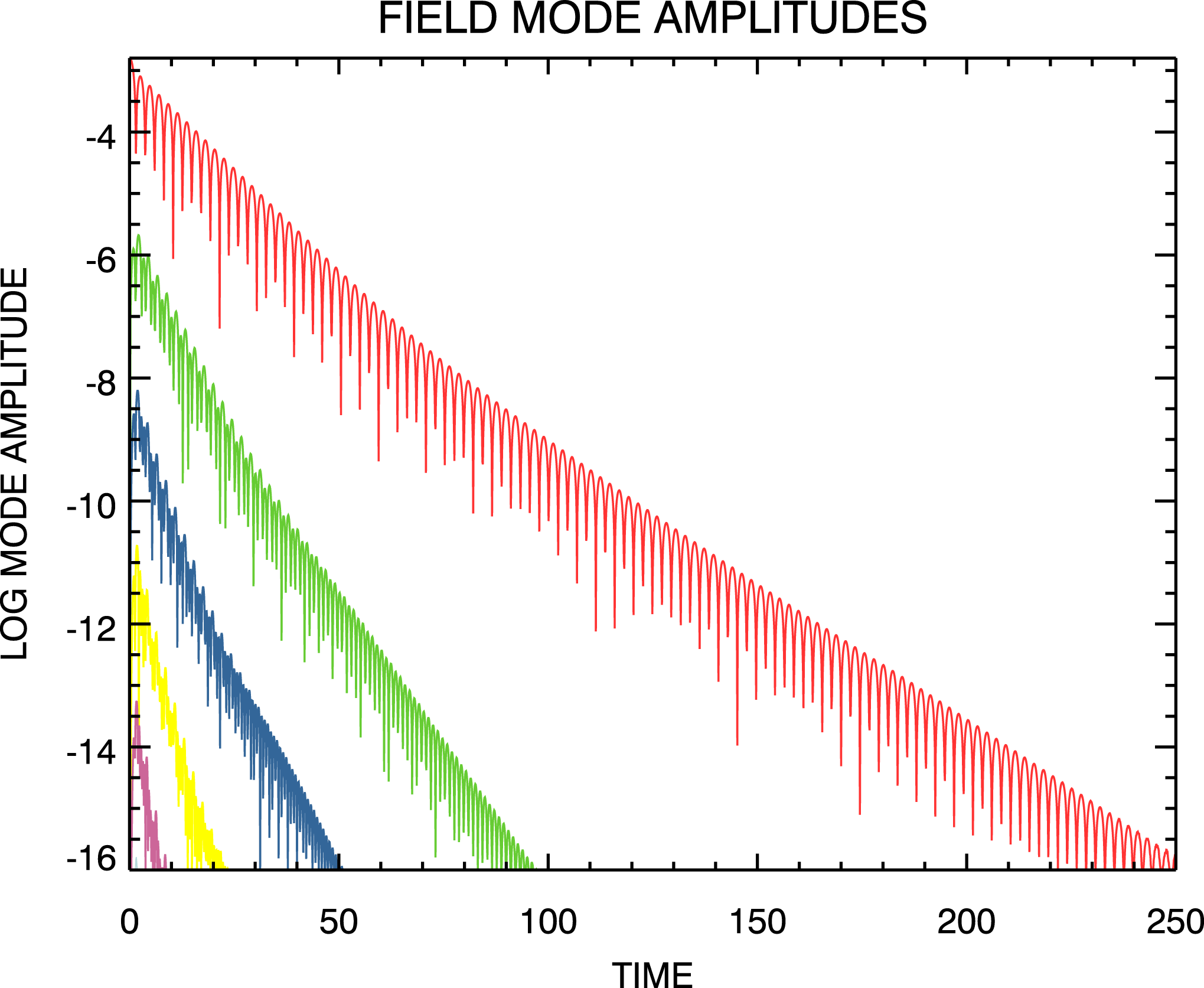
Time evolution of the electric field mode amplitudes from the filtered spectral Landau damping simulation using $\unicode[STIX]{x1D707}_{\max }=90$ and zeros inflow boundary data. Modes are ordered with decreasing amplitude with $m=1$ the dominant one.

Figure 9 shows the electric field mode amplitude evolution from a filtered spectral Landau damping simulation using the same initial state (3.1), $\unicode[STIX]{x1D707}_{\max }=90$ , $\unicode[STIX]{x1D707}_{0}=14.32$ and zeros for the inflow data at the $(\unicode[STIX]{x1D707}=\unicode[STIX]{x1D707}_{\max },m<0)$ boundary. It is important to note that, except for the change to inflow data filled with zeros at the $(\unicode[STIX]{x1D707}=\unicode[STIX]{x1D707}_{\max },m<0)$ boundary, the set-up for this simulation is identical to that that led to the recurrence dominated field mode evolution shown in figure 5. It appears that all of the recurrence effects have been removed. However, a comparison of this figure with the results shown in figure 7 from the extended $\unicode[STIX]{x1D707}$ -grid simulation shows a small reduction in the strength of the $m=1$ field mode at the end of the simulation.

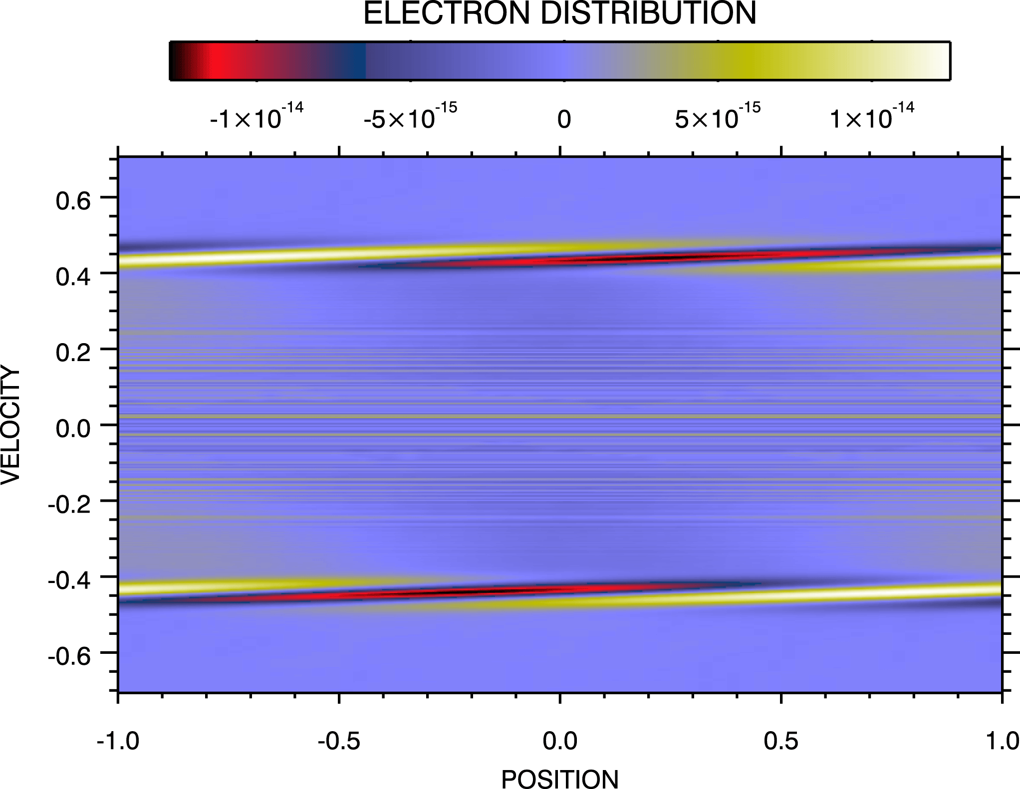
Figure 10 provides a comparison at $t=250$ of the perturbation on the phase-space distribution obtained from this simulation $(\unicode[STIX]{x1D707}_{\max }=90)$ with the perturbation obtained from the simulation carried out on the extended $\unicode[STIX]{x1D707}$ -grid $(\unicode[STIX]{x1D707}_{\max }=1900)$ shown in figure 8. Overall, the two distributions are in excellent agreement, with the $\unicode[STIX]{x1D707}_{\max }=90$ result showing a slight reduction in the strengths of the resonance disturbances, commensurate with the reduction in field strength at this time shown in figure 9. The ranges of the respective colour bars can be checked to confirm this reduction.

Figure 10.

Phase-space distribution with space-averaged component removed from the filtered spectral Landau damping simulation at $t=250$ using $\unicode[STIX]{x1D707}_{\max }=90$ and zeros inflow boundary data.

4.5 Spectral simulation, buffer input zeros, non-recurrent, $\unicode[STIX]{x1D707}_{\max }=200$

Figure 11.

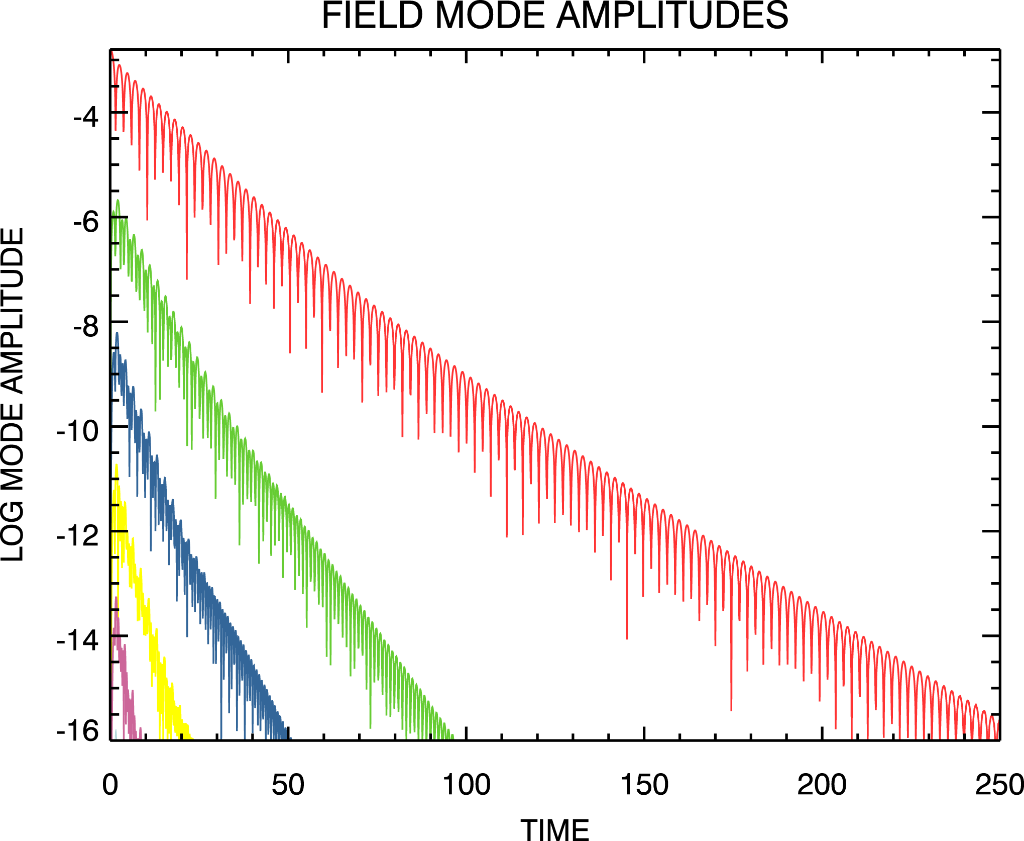
Time evolution of the electric field mode amplitudes from the filtered spectral Landau damping simulation using $\unicode[STIX]{x1D707}_{\max }=200$ and zeros inflow boundary data. Modes are ordered with decreasing amplitude with $m=1$ the dominant one.

Figure 11 shows the electric field mode amplitude evolution that results from increasing $\unicode[STIX]{x1D707}_{\max }$ to $\unicode[STIX]{x1D707}_{\max }=200$ while otherwise leaving the simulation set-up unchanged. Again, zeros for the inflow data at the $(\unicode[STIX]{x1D707}=\unicode[STIX]{x1D707}_{\max },m<0)$ boundary are used. With $\unicode[STIX]{x1D707}_{\max }=200$ , we find that even the small difference in the magnitude of the $m=1$ field mode at the end of the simulation has been removed.

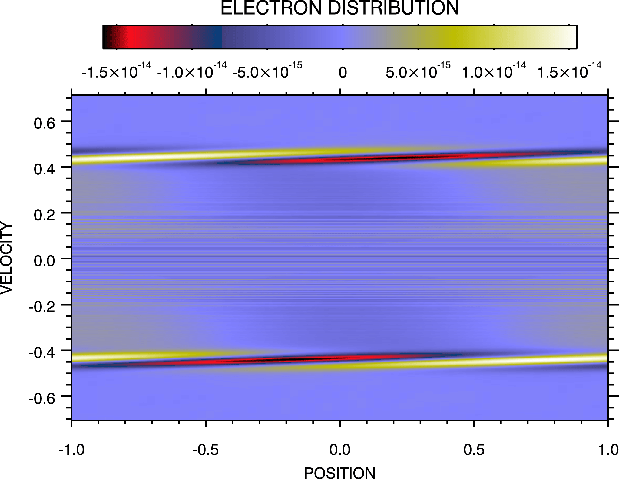
Figure 12 shows that with $\unicode[STIX]{x1D707}_{\max }=200$ the perturbation on the phase-space distribution at $t=250$ is now in excellent agreement with that of the extended $\unicode[STIX]{x1D707}$ -grid simulation. There appears to be no discernible differences between the results of these two simulations.

Figure 12.

Phase-space distribution with space-averaged component removed from the filtered spectral Landau damping simulation at $t=250$ using $\unicode[STIX]{x1D707}_{\max }=200$ and zeros inflow boundary data.

In summary:

1. (i) In this section, we have begun with a discussion of a spectral simulation in which the outflow of information at $(\unicode[STIX]{x1D707}=\unicode[STIX]{x1D707}_{\max },m>0)$ was recirculated to inflow at $(\unicode[STIX]{x1D707}=\unicode[STIX]{x1D707}_{\max },m<0)$ (§ 4.2). This was done to reproduce the periodic recirculation of information in the finite phase space of the flux-balance Landau damping simulation. It was necessary to choose $\unicode[STIX]{x1D707}_{\max }=90$ to reproduce the recurrence time $t_{\text{rec}}(1)=180$ of the flux-balance simulation. The strong recurrence effects obtained from these two distinct types of simulations, shown in figures 2 and 5 are in excellent agreement.

2. (ii) An extended $\unicode[STIX]{x1D707}$ -grid simulation was then discussed in which the recirculation of information at $\unicode[STIX]{x1D707}_{\max }$ was retained but the boundary was extended to $\unicode[STIX]{x1D707}_{\max }=1900$ (§ 4.3). This change is in exact analogy to the familiar reduction of $\unicode[STIX]{x0394}v$ , the velocity grid spacing, in an Eulerian simulation on a discretized $(x,v)$ -grid that is often employed to push all relevant recurrence times to beyond the range of the simulation. We then used the results of this simulation as a trusted basis for testing the accuracy two more spectral simulations in which a new method for removing recurrence was used.

3. (iii) In two spectral simulations, the recirculated inflow data at the $(\unicode[STIX]{x1D707}=\unicode[STIX]{x1D707}_{\max },m<0)$ boundary were replaced with zeros. For the first of these simulations we retained $\unicode[STIX]{x1D707}_{\max }=90$ (§ 4.4). All of the recurrence effects appeared removed and, except for small differences at the very end of the simulation in the $m=1$ field mode magnitude and the phase-space perturbation, the results appeared in excellent agreement with the results of the trusted extended $\unicode[STIX]{x1D707}$ -grid simulation.

4. (iv) For the second of these two spectral simulations with zeros for inflow data at the $(\unicode[STIX]{x1D707}=\unicode[STIX]{x1D707}_{\max },m<0)$ boundary, the $\unicode[STIX]{x1D707}$ -grid was extended to $\unicode[STIX]{x1D707}_{\max }=200$ (§ 4.5). In this case, excellent agreement with the trusted simulation was attained in all respects; there were no discrepancies at the end of the simulation.

Although not shown, we can confirm that several conservation rules were equally well satisfied by the three simulations discussed above in this § 4. It is a property of the spectral simulation code that the space-averaged electron density is exactly conserved and, so, this is true for the three simulations. All three simulations were initialized with zero space-averaged momentum and all three maintained zero space-averaged momentum to within machine precision. The total energies of all three simulations evolved in a similar manner while maintaining the initial value to within seven-digit accuracy. Higher-order quantities such as entropy or the L2 norm are not conserved by the filtered Vlasov equation. The conservation properties of these simulations indicate that the recurrence removal method that we propose does not introduce error in the simulations.

Thus, we will proceed in the next section to an application of these concepts to a published, very high velocity resolution, long-time, spectral Landau damping simulation.

Figure 13.

Time evolution of the electric field mode amplitudes from the spectral Landau damping transition simulation using $\unicode[STIX]{x1D707}_{\max }=3276.8$ and zeros inflow boundary data. Taken from Klimas et al. (Reference Klimas, Vinas and Araneda2017). Modes are ordered with decreasing amplitude with $m=1$ the dominant one.

4.6 Spectral transition simulation, buffer input zeros, non-recurrent, $\unicode[STIX]{x1D707}_{\max }=3276.8$

Figure 13 (taken from Klimas et al. (Reference Klimas, Vinas and Araneda2017)) shows the time evolution of the field mode magnitudes from a spectral simulation of a Landau damping ‘transition’ simulation. In terms of the dimensionless variables defined in § 2.2, following Rupp, Lopez & Araneda (Reference Rupp, Lopez and Araneda2015) the simulation was initialized with

(4.1) $$\begin{eqnarray}f(x,v,t=0)=\left(\unicode[STIX]{x03C0}\frac{c}{v_{th}}\right)\frac{1}{\sqrt{2\unicode[STIX]{x03C0}}}\text{e}^{-1/2(\unicode[STIX]{x03C0}(c/v_{th}))^{2}v^{2}}[1+\unicode[STIX]{x1D700}\cos \unicode[STIX]{x03C0}x]\end{eqnarray}$$

using $v_{th}/c=0.4$ . The neighbourhood of the transition from persisting to arrested Landau damping was explored by varying the value of $\unicode[STIX]{x1D700}$ . The results shown in figure 13 are for $\unicode[STIX]{x1D700}$ very near to its transition value, in which case the fundamental $m=1$ field mode asymptotes to a constant average value with increasing time. Slightly higher values for $\unicode[STIX]{x1D700}$ lead to an ‘arrest’ of the initial damping, a shift to Landau growth, and finally to a saturated state in which the field mode magnitudes fluctuate substantially about respective asymptotic values. Slightly lower values for $\unicode[STIX]{x1D700}$ lead to continuing Landau damping, as in, e.g. figure 11. Rupp et al. (Reference Rupp, Lopez and Araneda2015) examined the $\unicode[STIX]{x1D700}$ -neighbourhood just above the transition value $\unicode[STIX]{x1D700}_{\text{tran}}$ and showed that the arrest and saturation times are particular power-law functions of $\unicode[STIX]{x1D700}-\unicode[STIX]{x1D700}_{\text{tran}}$ that indicate the transition from arrested to persisting Landau damping is a second-order phase transition.

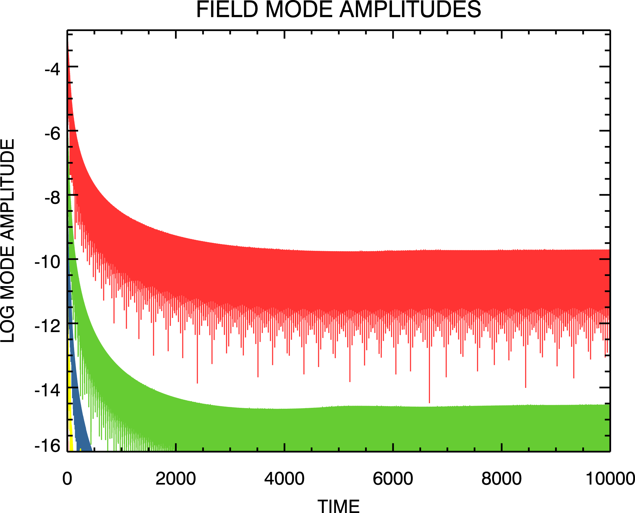
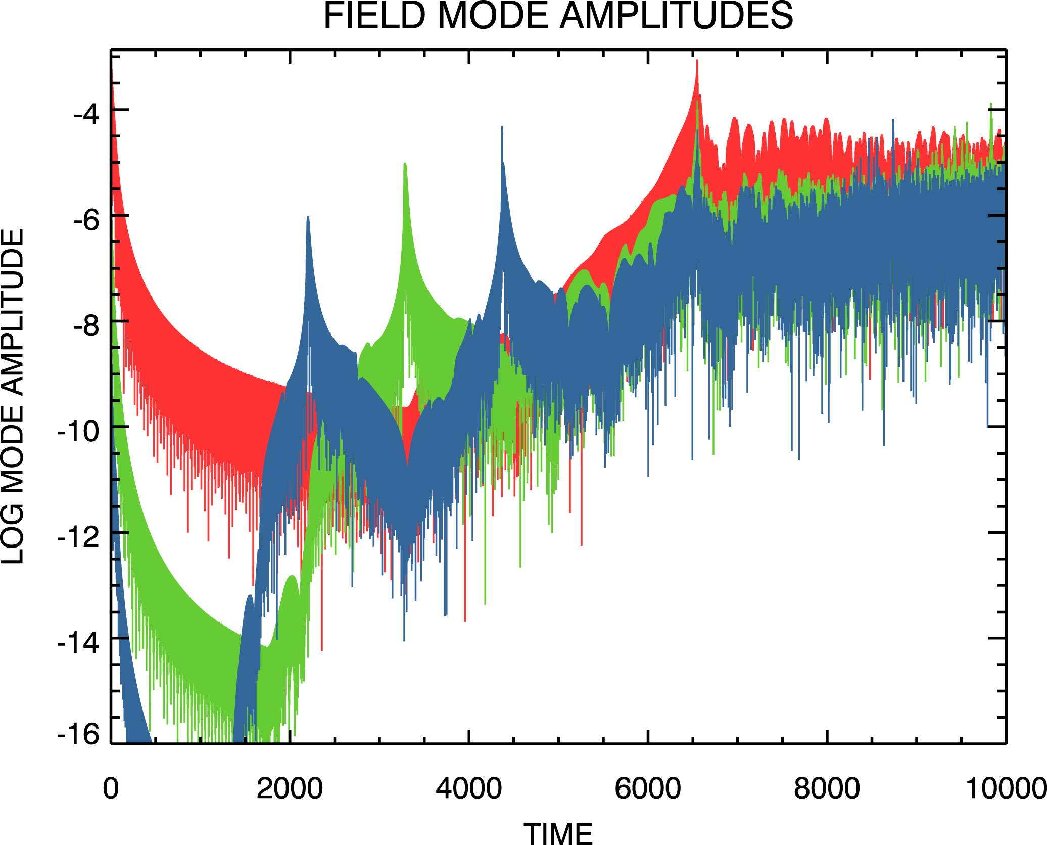
For the purposes of the transition study, very high velocity resolution was required. Accordingly, an extended $\unicode[STIX]{x1D707}$ -grid was used with $\unicode[STIX]{x1D707}_{\max }=3276.8$ . Of relevance to this discussion, however, is the implied $t_{\text{rec}}(1)\simeq 6600$ , which is less than the maximum time $t_{\max }=10\,000$ reached by the simulation. To obtain the field mode magnitude evolution shown in figure 14 we have reproduced the transition simulation due to Klimas et al. (Reference Klimas, Vinas and Araneda2017) but with recirculated inflow data at the $(\unicode[STIX]{x1D707}=\unicode[STIX]{x1D707}_{\max },m<0)$ boundary, thus leading to the recurrence effects that are shown in the figure. It can be seen that the recurrence effects invalidate most of the simulation and that we have confirmed $t_{\text{rec}}(1)\simeq 6600$ .

Figure 14.

Time evolution of the three longest wavelength electric field mode amplitudes from the spectral Landau damping transition simulation using $\unicode[STIX]{x1D707}_{\max }=3276.8$ and recirculated inflow boundary data. Modes are ordered with decreasing amplitude with $m=1$ the one shown in red.

We would argue that figure 13, from the transition study of Klimas et al. (Reference Klimas, Vinas and Araneda2017), does not exhibit any effects of recurrence. This, while $\unicode[STIX]{x1D707}_{\max }$ is not so large that all relevant recurrence times have been pushed beyond the range of the simulation. We can conclude that unmanageable increases in $\unicode[STIX]{x1D707}_{\max }$ , analogous to unmanageable decreases in $\unicode[STIX]{x0394}v$ in discretized $(x,v)$ -based simulations, are not required to remove recurrence effects from arbitrarily long Vlasov–Poisson spectral simulations.

The transition simulation was carried out using the recurrence-free set-up, zeros filling the inflow data at the $(\unicode[STIX]{x1D707}=\unicode[STIX]{x1D707}_{\max },m<0)$ boundary and steady outflow at the $(\unicode[STIX]{x1D707}=\unicode[STIX]{x1D707}_{\max },m>0)$ boundary. We have examined the evolution of the spectral phase-space distribution that follows with these boundary conditions in place.

Figure 15.

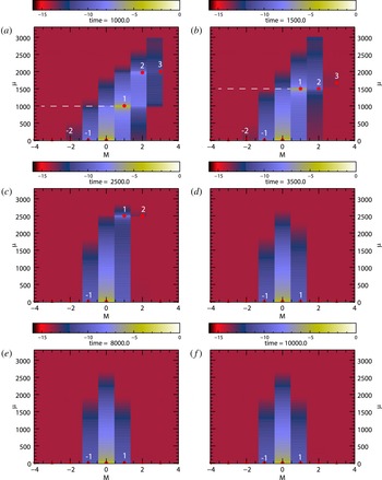
Spectral representations of phase-space distribution at selected times from transition simulation taken directly from spectral code. Red stars show positions of peak values in the individual modes. Numbers indicate mode numbers.

Figure 15 shows spectral phase-space distributions at selected times obtained from the recurrence-free transition simulation of Klimas et al. (Reference Klimas, Vinas and Araneda2017), the simulation whose field mode amplitudes are displayed in figure 13. At the earliest time shown (a, $t=1000$ ) all of the higher Fourier modes on the $m>0$ side of the distribution have already propagated beyond $\unicode[STIX]{x1D707}_{\max }$ and off the grid, leaving only the $m=1{-}3$ modes. Comparing (a,b), it can be seen that as the peak in the $m=1$ mode propagates to higher $\unicode[STIX]{x1D707}$ -values, the $m=-1$ mode distribution also expands in the same direction; this, despite the downward information flow in the $m=-1$ mode. We believe that this behaviour indicates a transfer of information from the $m=1$ mode to the $m=-1$ mode, perhaps through mode–mode coupling involving the $m=0,\pm 1$ modes. At $t=2500$ (c), the peak in the $m=1$ mode approaches $\unicode[STIX]{x1D707}_{\max }$ and the $m=-1$ distribution continues to expand upward. At $t=3500$ (d), following the passage of the $m=1$ peak off the grid, the $m=1$ distribution shrinks back as the $m=-1$ continues expanding slightly. By $t=8000$ (e), the two $m=\pm 1$ modes have come into equilibrium and there is no further evolution up to the end of the simulation at $t=10\,000$ (f). We speculate that this steady state is maintained through a continuous cycling of information; upward in the $m>0$ region, downward in the $m<0$ region and across the $m=0$ axis through mode–mode coupling (recycling of information at $\unicode[STIX]{x1D707}=0$ from $m<0$ to $m>0$ using the reality condition is always in effect). The inflow of zeros at the $(\unicode[STIX]{x1D707}=\unicode[STIX]{x1D707}_{\max },m<0)$ boundary is matched by an outflow of zeros at the $(\unicode[STIX]{x1D707}=\unicode[STIX]{x1D707}_{\max },m>0)$ boundary, the zeros at this boundary being due to the depression of the outflow data enforced by the Gaussian tail of the filamentation filter. Recycling governed by the plasma physics of mode–mode coupling up and down the $m=0$ axis has replaced the periodic recycling of information at the $(\unicode[STIX]{x1D707}=\unicode[STIX]{x1D707}_{\max },m<0)$ boundary that leads to recurrence. A recurrence-free, long-time simulation results.