1. Introduction
There exist numerous geological scenarios where a dense or light source fluid is injected into a saturated, sedimentary porous medium that is, in lateral extent, either confined or effectively unconfined. In the former case, lateral boundaries may be associated with an anticlinal concave-down geometry or with sealing faults. Such boundaries are expected to exert a non-trivial influence on the evolution of the injectate be this associated with geothermal storage (MacKay Reference MacKay2009; Paksoy & Beyhan Reference Paksoy and Beyhan2014), hydrogen storage (Feldmann et al. Reference Feldmann, Hagemann, Ganzer and Panfilov2016; Sainz-Garcia Reference Sainz-Garcia2017; Tarkowski Reference Tarkowski2019), the sequestration of acid-gas in abandoned oil wells (Bachu & Gunter Reference Bachu and Gunter2004; Wu & Carroll Reference Wu and Carroll2011) or the sequestration of supercritical  $\textrm {CO}_2$ in deep saline aquifers (Torp & Gale Reference Torp and Gale2004; Ajayi, Gomes & Bera Reference Ajayi, Gomes and Bera2019; Michael et al. Reference Michael, Golab, Shulakova, Ennis-King, Allinson, Sharma and Aiken2010).
For each of the above examples, a critical consideration is that of storage security, which requires, in turn, an assessment of the likelihood of injectate leakage. Such leakage may arise from inadequate seals (i.e. a geological boundary that is semipermeable), filling a formation to capacity or leakage faults along the spreading boundary (Flett, Gurton & Taggart Reference Flett, Gurton and Taggart2005). Our present focus is on the former instance, i.e. we consider that the bounding layer along which the injectate spreads does not altogether arrest vertical migration. Such a scenario, arises, for example, with the (albeit thin) layers of mudstone that are present within the Utsira Sand, the otherwise sandstone layer of thickness 200 m to 300 m into which supercritical  $\textrm {CO}_2$ from the Sleipner project is injected (Mouche, Hayek & Mügler Reference Mouche, Hayek and Mügler2010; Boait et al. Reference Boait, White, Bickle, Chadwick, Neufeld and Huppert2012). The scenario in question is relevant to other examples of heterogeneous porous media e.g. the sandstone layers separated by tight interlayers of comparable thickness considered in figure 5 of the hydrogen storage study of Feldmann et al. (Reference Feldmann, Hagemann, Ganzer and Panfilov2016). To predict the long-term fate of the injectate, it is important to predict the flow behaviour along such leaky boundaries. Previous work (cited below) has emphasized the prediction of early-time dynamics such that the depth of the low-permeable bounding layer is immaterial. Here, we relax this limitation and consider longer time horizons assuming bounding layers of intermediate thickness. In so doing, we demonstrate that the bounding layer depth (plus additional details such as the source conditions and inclination angle of the permeability jump) dictate the manner in which the (multilayer) porous medium fills with injected fluid.
Common also to most of the examples cited above is that they combine the end-member states of buoyancy-driven flow, i.e. a vertical plume that, upon striking an impermeable or semi-impermeable boundary, feeds a horizontal (or nearly horizontal) gravity current. Although the plume may traverse only a modest vertical length compared with the long horizontal distances travelled by the gravity current, significant entrainment of external ambient fluid may nonetheless occur. This is especially true when the injectate and ambient fluid are miscible, e.g. a plume of  $\textrm {H}_2$ rising through a cushion gas layer of
 $\textrm {CH}_4$ or
 $\textrm {N}_2$ (Feldmann et al. Reference Feldmann, Hagemann, Ganzer and Panfilov2016) or when the plume is deflected e.g. as a result of a background mean flow (Weaver & Wilson Reference Weaver and Wilson2000; Van Stempvoort et al. Reference Van Stempvoort, Roy, Grabuski, Brown, Bickerton and Sverko2013) and/or stratigraphic steering (Morgan et al. Reference Morgan, Kent, Seitz and Novak2008; Kamath et al. Reference Kamath, Connor, McHugh, Nemir, Le and Ryan2012). In the idealized case where viscosity contrasts are small, the equations describing entrainment into a vertical plume are derived by Wooding (Reference Wooding1963), this for the scenario of a deep, uniform porous medium and a diffusion-dominated Darcy flow characterized by low Péclét number, i.e.
 ${Pe} \lesssim O(1)$. Sahu & Flynn (Reference Sahu and Flynn2015) present equations analogous to Wooding's but for the case
 $Pe\gg O(1)$ in which circumstance dispersion dominates over diffusion.
In contrast to porous media plumes, more attention has been devoted to porous media gravity currents, whether these flow along boundaries are categorized as impermeable (Huppert & Woods Reference Huppert and Woods1995; Vella & Huppert Reference Vella and Huppert2006), semi-impermeable (Vella et al. Reference Vella, Neufeld, Huppert and Lister2011; Farcas & Woods Reference Farcas and Woods2013) or permeable (Pritchard, Woods & Hogg Reference Pritchard, Woods and Hogg2001; Farcas & Woods Reference Farcas and Woods2009; Goda & Sato Reference Goda and Sato2011). As regards the latter two scenarios, and assuming a gravity current of dense fluid, studies have sought to characterize the dynamical impact of basal draining be this owing to a point sink or fissure (Neufeld, Vella & Huppert Reference Neufeld, Vella and Huppert2009; Neufeld et al. Reference Neufeld, Vella, Huppert and Lister2011; Vella et al. Reference Vella, Neufeld, Huppert and Lister2011; Farcas & Woods Reference Farcas and Woods2013), edge drainage (Hesse & Woods Reference Hesse and Woods2010; Rayward-Smith & Woods Reference Rayward-Smith and Woods2011; Zheng et al. Reference Zheng, Soh, Huppert and Stone2013; Hagemann, Panfilov & Ganzer Reference Hagemann, Panfilov and Ganzer2016) or distributed leakage (Pritchard et al. Reference Pritchard, Woods and Hogg2001; Neufeld & Huppert Reference Neufeld and Huppert2009; Farcas & Woods Reference Farcas and Woods2009; Woods & Farcas Reference Woods and Farcas2009; Yu, Zheng & Stone Reference Yu, Zheng and Stone2017). Consistent with the preceding discussion, detailed characterizations should consider the depth of the lower layer, i.e. the layer into which fluid discharged by the gravity current drains. Arguably the simplest configuration assumes a lower layer that is infinitely deep, a case studied in precise analytical detail by Goda & Sato (Reference Goda and Sato2011). They examined a sharp permeability jump separating layers of comparatively large versus small permeability. In adapting the analysis of Huppert & Woods (Reference Huppert and Woods1995) and Pritchard et al. (Reference Pritchard, Woods and Hogg2001), Goda & Sato (Reference Goda and Sato2011) derived coupled nonlinear advection equations describing the gravity current and draining flows. By solving these equations numerically, they demonstrated that gravity currents propagating along a permeability jump will eventually reach a terminal, or runout, length. Runout occurs when the influx to the gravity current matches the rate of basal draining into the lower layer. (Consistent with the orientation relevant to geological sequestration, Goda & Sato (Reference Goda and Sato2011) assumed a buoyant gravity current travelling along the underside of a permeability jump. As such, fluid drained from the gravity current into the upper, not the lower, layer. We prefer to consider a dense gravity current so as to be consistent with numerous other studies e.g. Pritchard et al. (Reference Pritchard, Woods and Hogg2001), Lyle et al. (Reference Lyle, Huppert, Hallworth, Bicle and Chadwick2005), Vella & Huppert (Reference Vella and Huppert2006), De Loubens & Ramakrishnan (Reference De Loubens and Ramakrishnan2011), Sahu & Flynn (Reference Sahu and Flynn2015, Reference Sahu and Flynn2016, Reference Sahu and Flynn2017) and also the experiments to be reported upon in §§ 2 to 4. The experiments performed in this study consider small density differences between the source and ambient fluids and, therefore, the flow remains Boussinesq everywhere in the domain. In such cases, the flow orientation, i.e. upward vs downward, is immaterial.) The theoretical study of Goda & Sato (Reference Goda and Sato2011) was broadened by later theoretical and experimental work conducted by Sahu & Flynn (Reference Sahu and Flynn2017). Sahu & Flynn (Reference Sahu and Flynn2017) made their upper and lower layers finite in horizontal and vertical extent and thereby additionally studied the time scales for layer filling by contaminated fluid. In this respect, the study of Sahu & Flynn (Reference Sahu and Flynn2017) was motivated by a desire to characterize the geological utility of ‘filling box’ models. Originally studied in the non-porous media context (i.e. ‘a plume in a room’), filling box models describe the spatio-temporal evolution of buoyancy within a closed (Baines & Turner Reference Baines and Turner1969) or ventilated (Caulfield & Woods Reference Caulfield and Woods2002) control volume subject to localized heating or cooling. Although filling box models have been applied to problems of ocean circulation (Manins Reference Manins1979; Speer & Tziperman Reference Speer and Tziperman1990; Hughes & Griffiths Reference Hughes and Griffiths2006), they have received less attention in the context of porous media flows in general and sequestration/storage flows in particular. This lack of attention is surprising given the natural ability of filling box models to describe the dynamical importance of boundaries in the context of reservoirs/aquifers.
Expanding on the study by Sahu & Flynn (Reference Sahu and Flynn2017) on porous media filling box models, we herein extend the analysis to situations of greater geological realism. For instance, a key characteristic of the experiments of Sahu & Flynn (Reference Sahu and Flynn2017) is that the permeability jump is horizontal. On the other hand, there are many instances where, in modelling real geological flows, it would be more appropriate to consider a permeability jump that is either sloping (Bachu et al. Reference Bachu, Buschkuehle, Haug and Michael2008a,Reference Bachu, Buschkuehle, Haug and Michaelb; MacMinn, Szulczewski & Juanes Reference MacMinn, Szulczewski and Juanes2010) or curved (Ajayi et al. Reference Ajayi, Gomes and Bera2019). The former complication was incorporated into the recent theoretical study of Bharath, Sahu & Flynn (Reference Bharath, Sahu and Flynn2020). They consider up- and downdip gravity currents fed by a descending plume rather than by a source located along the permeability jump. In turn, their model captures the early-time spreading dynamics by predicting the flow evolution up to the point of runout. On the other hand, the theory and laboratory experiments reported by Bharath et al. (Reference Bharath, Sahu and Flynn2020) do not provide meaningful insights into the longer term dynamics and how these are influenced by (i) the depth of the lower layer, and (ii) the presence of sidewall boundaries. To this end, the experiments described in this study provide an especially interesting vantage point from which to study filling box dynamics because of the appearance of primary and secondary gravity currents. These arise, respectively, along the permeability jump and along the bottom (impermeable) boundary. The relative motion of the primary versus secondary gravity currents was ignored by Sahu & Flynn (Reference Sahu and Flynn2017) but has, as we shall see, a crucial influence on the manner in which the heterogeneous porous medium becomes filled with contaminated fluid. Because medium filling is closely related to medium storage efficiencies and the long-term fate of the injectate, it is important to be able to characterize the manner and speed with which the lower versus upper layers are filled. Addressing such topics is a further objective of this study.
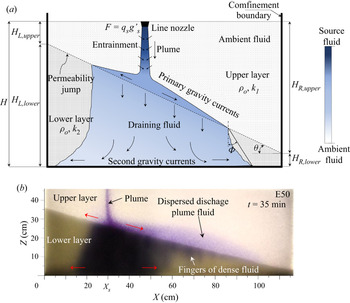
Throughout, we pursue an experimental approach and examine the evolution of the flow, exhibited schematically in figure 1(a). Dense fluid, dyed for ease of visualization, is discharged by a line source and then propagates downward through the upper layer until it strikes the permeability jump. There follows drainage of discharged plume fluid into the lower layer and the formation and propagation of the primary and secondary gravity currents. Because the box in which experiments are performed is relatively thin in the spanwise direction, the flow is largely two-dimensional (2-D), i.e. there is limited opportunity for spanwise flow instabilities to develop. In addition, the dynamic viscosities of the injected and ambient fluids are considered identical. These fluids being additionally fully miscible, we neglect surface tension effects and assume infinitely large values for the Bond number, which characterizes the ratio of buoyancy to capillarity. In this respect, our approach is consistent with numerous previous studies (Huppert & Woods Reference Huppert and Woods1995; Rayward-Smith & Woods Reference Rayward-Smith and Woods2011; Szulczewski & Juanes Reference Szulczewski and Juanes2013; Pegler, Huppert & Neufeld Reference Pegler, Huppert and Neufeld2016).
(a) Schematic showing discharged plume fluid propagating as a pair of primary and secondary currents in the upper and lower layers, respectively. The colour bar indicates the variation of fluid density as the source fluid propagates through the heterogeneous porous medium. (b) Analogue snapshot image from our laboratory experiments. Here,  $X_s$ on the horizontal axis indicates the position of the nozzle.

The rest of our manuscript is outlined as follows: in § 2, the experimental procedure is outlined as is our method for post-processing experimental images and analysing the resulting measured data. In § 3, qualitative and quantitative analyses of the primarily horizontal flows in the upper and lower layers are made. The counterpart vertical and filling box flows are examined in § 4. The mutual dependence of horizontal and vertical flows during the filling process is discussed in § 5. Finally, in § 6 we summarize and discuss the key findings and applications of this study.
2. Experimental procedure
2.1. Experimental set-up
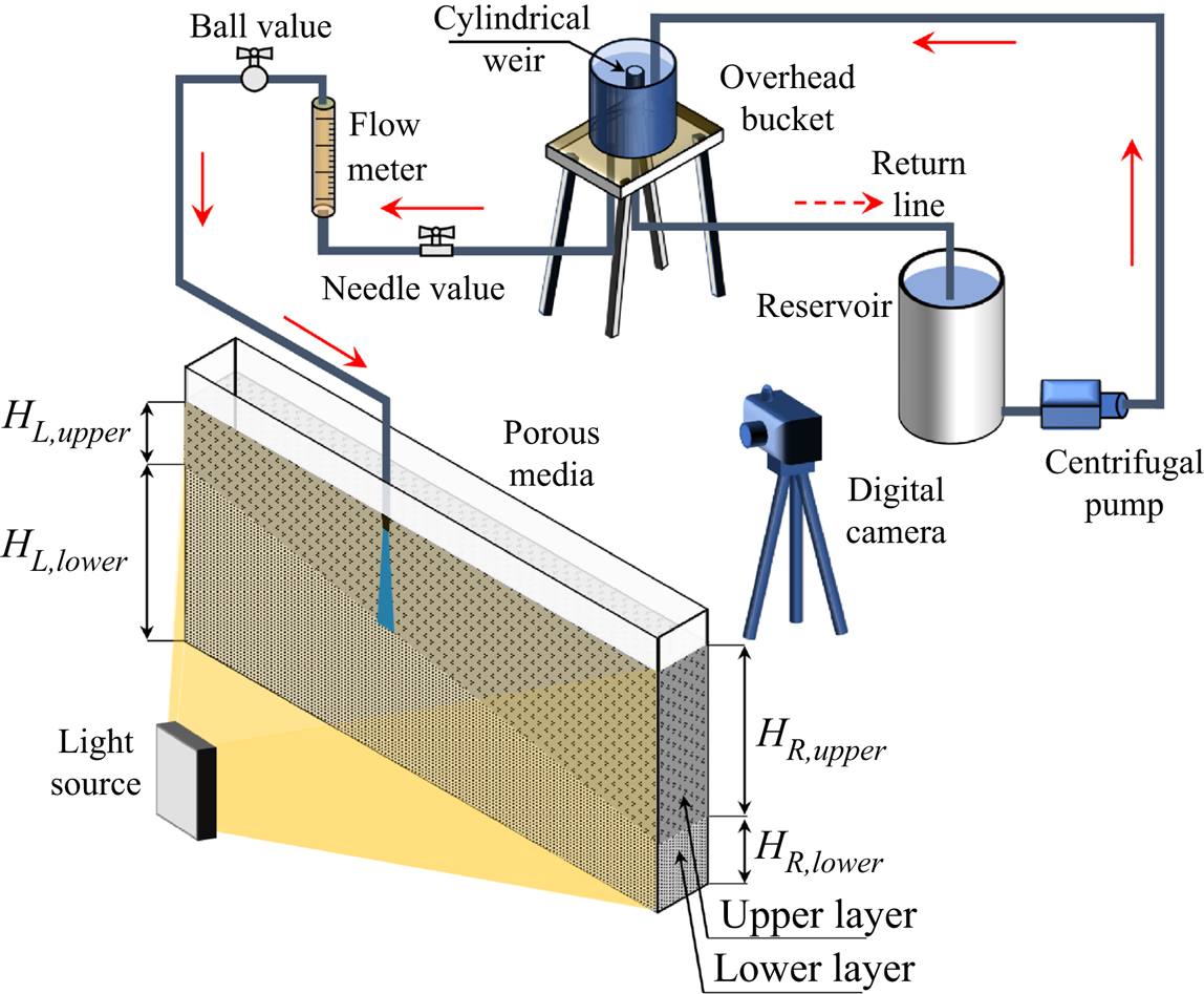
Experiments were performed using a transparent rectangular box of dimensions  $118\ \textrm {cm}\ \textrm {long} \times 7.6\ \textrm {cm}\ \textrm {wide} \times 60\ \textrm {cm}$ deep filled with spherical beads (Potters Industries A Series Premium) as shown in figure 2. The beads in the upper layer were
 $d_1=3.0\pm 0.2\ \textrm {mm}$ in diameter and those in the lower layer were
 $d_2=1.0\pm 0.2\ \textrm {mm}$ in diameter. The bead density, as specified by the manufacturer, was
 $1.54\ \textrm {g}\ \textrm {cm}^{-3}$. The entire porous medium was saturated with tap water having a density of approximately
 $\rho _o = 0.998\ \textrm {g}\ \textrm {cm}^{-3}$. The layers were separated by a distinct interface, which we refer to as the permeability jump. Upper and lower layer permeabilities were determined based on the empirical relationship proposed by Kozeny and Carman, and discussed by Dullien (Reference Dullien1979), i.e.
 \begin{equation} k_i= \frac {d_i^2 \phi^{3}}{180(1-\phi)^2} \end{equation}
where  $i=1$, 2 corresponds to the upper and lower layer, respectively. For all experiments conducted here, the value of the permeability ratio,
 $K=k_2/k_1 \propto d_2^2/d_1^2$ was kept fixed at 0.11. The heterogeneous medium was varied by changing the angle,
 $\theta$, of the permeability jump, which, in turn, had the effect of changing the vertical distances
 $H_{L,{upper}}$,
 $H_{L,{lower}}$,
 $H_{R,{upper}}$,
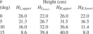
 $H_{R,{lower}}$ defined schematically in figure 1(a) and quantitatively in table 1. In all cases,
 $H_{L,{lower}} + H_{L,{upper}} = H_{R,{lower}} + H_{R,{upper}} = H = 47\ \textrm {cm}$ where
 $H$ represents the combined depth of the upper and lower layers.
Schematic of the experimental set-up.

Porous media dimensions. Heights are considered accurate to within  $\pm 0.5\ \textrm {cm}$ and angles are considered accurate to within
 $\pm 0.2^{\circ }$.

As depicted in figure 2, dense source fluid was supplied at the top of the upper layer using a line source nozzle that spanned the tank width of 6.45 cm. The nozzle was designed in such a manner that it produced a uniform flow along its length even at small flow rates (Roes Reference Roes2014). For each of the permeability jump angles prescribed in table 1, experiments were performed by positioning the nozzle (source) at various horizontal locations. Using non-dimensional variables, the source location was characterized by  $X_s^*=X_s/L$, where
 $L = 118\ \textrm {cm}$ is the inside box length and
 $X_s$ is the corresponding horizontal position of the nozzle midplane measured relative to the updip end wall. Adjusting the nozzle location allowed us to perform experiments for various effective lower layer depths and to study the influence of sidewall boundaries on the flow behaviour.
Dense source fluid was prepared by mixing a precalculated mass of salt into tap water in a 100 L reservoir. The density of the resulting solution,  $\rho _s$, was measured to an accuracy of
 $0.00005\ \textrm {g}\ \textrm {cm}^{-3}$ using an Anton Paar DMA 4500 densitometer. Moreover, and for purposes of flow visualization, a small amount of cold-water dye (Procion MX) was added to the saltwater solution. The dye concentration (determined with reference to the calibration curves of Appendix B) was small enough that it did not significantly alter the plume source density. The dyed, saltwater was then pumped into an overhead bucket using a centrifugal pump (Little Gaint Pump Co., Model 3-MD). Inside of the bucket was placed a cylindrical weir whose purpose was to maintain a constant elevation of fluid inside the bucket. Fluid flowing over the weir was returned to the reservoir thereby assuring well-mixed conditions over the 3 to 5 h duration of each experiment. Fluid not flowing over the weir was discharged through 12.7 mm inner diameter tubing to the plume nozzle after first passing through a flow-control needle valve (0.5 inch, Swagelok SS-8GUF8), a flow meter (Gilmont GV-2119-S-P) and an on/off ball valve (0.5 inch, Kebechem). The flow parameters of interest were the source volume flux,
 $Q_s$, and the source reduced gravity,
 $g'_s= g (\rho _s-\rho _o)/\rho _o\ll g$, where
 $g$ is gravitational acceleration. A detailed list of experimental parameters for different source conditions and porous media configurations is described in table 2 of Appendix A.
2.2. Image capture
Experimental snapshots were captured using a Canon Rebel EOS T2i 18.0 PM with an 18–55 mm IS II zoom lens, which collected images every 30 s. Uniform intensity backlighting was achieved using a 3M 1880 overhead projector, whose head was situated at the box centre, i.e. at respective horizontal and vertical distances of 60 cm and 25 cm from the box lower left hand corner. The projector was located 150 cm behind the box. The backside of the box was covered with tracing paper, which served to diffuse the incoming light. Images captured using the Canon Rebel camera were standard RGB,  $720\times 400$ pixels in size and had a resolution of 72 dpi. They were post-processed in Matlab where all of the images corresponding to a particular experimental set were first cropped to remove unwanted regions outside of the flow domain. The images were then corrected by subtracting away a reference image (collected before the initiation of flow). This step removed any systematic spatial variations in the light intensity e.g. arising from some localized ‘dark spot’ within the bead pack. Finally, images were converted to false-colour and the pixel intensities were normalized so that they ranged from 0 to 1.
2.3. Analysis of snapshot and time series images
A true-colour snapshot of an experiment with  $\theta =15^\circ$ is shown in figure 1(b). The source conditions measure
 $Q_s = 1.01 \pm 0.02\ \textrm {cm}^{3}\ \textrm {s}^{-1}$ and
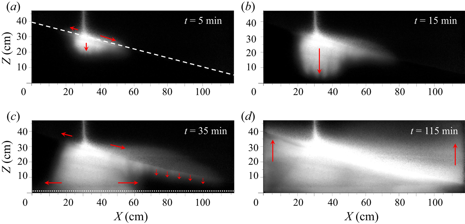
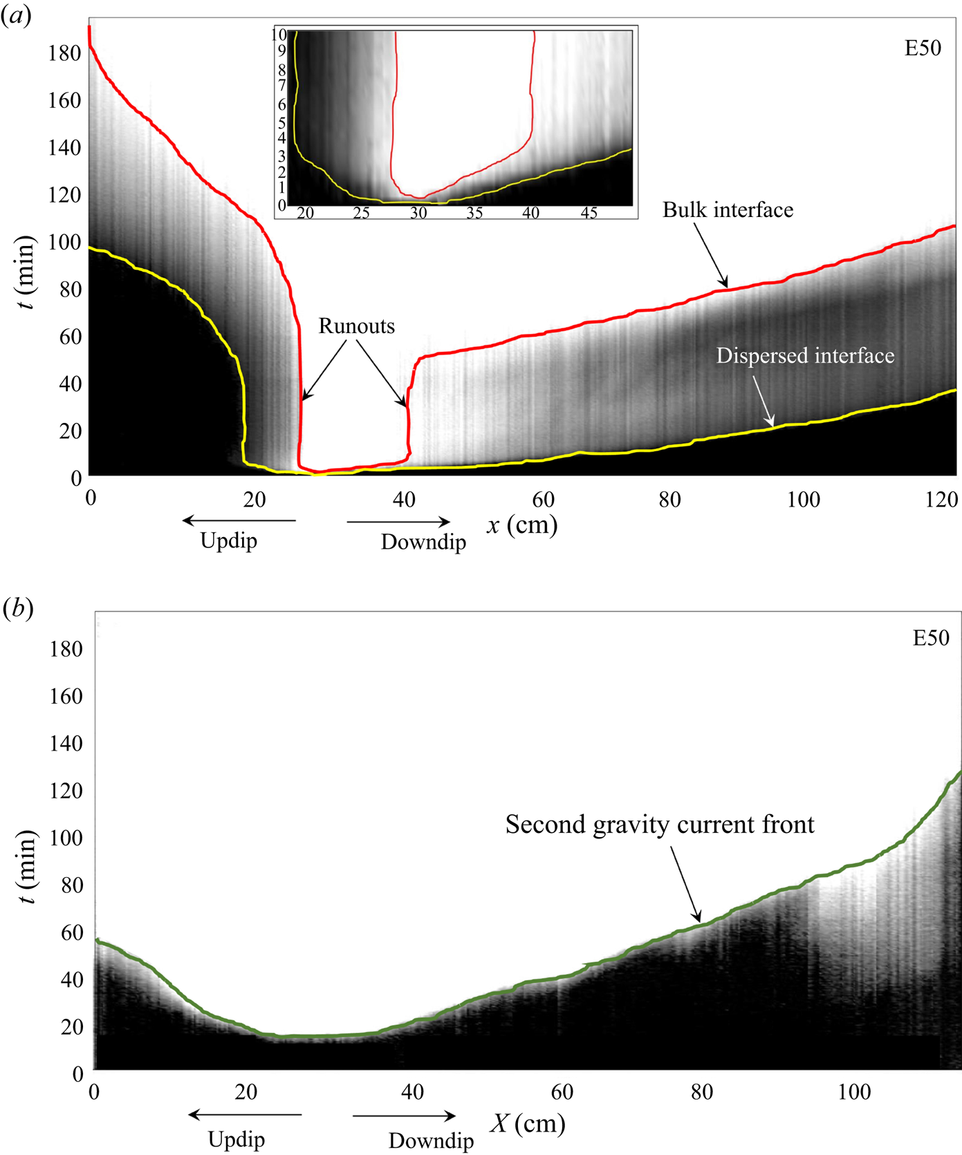
 $g'_s = 20.1\pm 0.9\ \textrm {cm}\ \textrm {s}^{-2}$ – see E50 in table 2. Figure 3 shows a sequence of false-colour snapshot images for this case. The source fluid from the nozzle descends as a negatively buoyant plume from the nozzle. The plume fluid, upon striking the permeability jump, propagates either up- or downdip as a leaky gravity current or else drains directly into the lower layer, as shown in figure 3(a). The along-slope flow dynamics of the primary gravity currents are studied by plotting the nose positions, both up- and downdip, as functions of time. Facilitating this process, we construct ITS images using the methodology summarized by Bharath et al. (Reference Bharath, Sahu and Flynn2020). In brief, a diagonal line of slope
 $\tan \theta$ is drawn two or three pixels above the permeability jump. From the sequence of snapshot images, we then track the change of pixel intensity along this diagonal line, a process that results in ITS images such as that of figure 4(a). In contrast to the snapshot images of figure 3, which make reference to horizontal (
 $X$) and vertical (
 $Z$) coordinates, ITS images measure the flow evolution with reference to an along-slope coordinate,
 $x=X/\cos \theta$. Note that, in figure 4(a),
 $x_s=25.9\ \textrm {cm}$ is defined to coincide with the location of the nozzle (located at
 $X_s=25.0\ \textrm {cm}$) so that
 $x_s<25.9\ \textrm {cm}$ and
 $x_s>25.9\ \textrm {cm}$ correspond, respectively, to the up- and downdip directions.
Snapshot images (false-colour) for  $\theta =15^\circ$ with source conditions
 $Q_s = 1.01 \pm 0.02\ \textrm {cm}^{3}\ \textrm {s}^{-1}$ and
 $g'_s = 20.1\pm 0.9\ \textrm {cm}\ \textrm {s}^{-2}$ illustrating the time evolution of a canonical experiment. (a) Fluid discharged by the plume propagates as a pair of up- and downdip primary gravity currents and also drains into the lower layer. (b) A greater fraction of the discharged plume fluid drains into the lower layer as the primary gravity currents approach their respective runout lengths. (c) Formation of secondary gravity currents following contact by the draining fluid with the bottom (impermeable) boundary. The remobilization of the primary gravity currents occurs thereafter. (d) Vertical advection of discharged plume fluid towards the source, which occurs after the primary and secondary gravity currents reach the box sidewalls. The filling process is characterized by a ‘first front’ that separates contaminated fluid (below) from uncontaminated ambient fluid (above). In all panels, arrows show the dominant flow directions. The dashed line of (a) and the dotted line of (c) respectively indicate the lines along which inclined time series (ITS, e.g. figure 4a) and horizontal time series (HTS; e.g. figure 4b) images are collected.

(a) ITS image and (b) HTS image, constructed from 390 snapshot images corresponding to the experiment of figure 3 and used to analyse the up- and downdip propagation of the primary and secondary gravity currents. The meaning of the red and yellow contours in (a) and of the green contour in (b) is explained in the text. The inset figure in (a) illustrates the flow behaviour at early times.

Figure 4(a) is derived from figure 3 and includes two contour lines. The red contour corresponds to the primary gravity current ‘bulk interface’, and indicates the boundary above which the pixel intensity is both large and nearly uniform in space and time. As described in quantitative detail in Appendix B, we consider the solute concentration to be a direct function of the dye concentration. Because the solute concentration is a surrogate for the fluid density, we surmise that the density (or reduced gravity) of the fluid above the red contour is approximately uniform. We refer to the fluid appearing above the red contour as the bulk fluid. Conversely, the yellow contour of figure 4(a) is referred to as the ‘dispersed interface’; it separates uncontaminated ambient fluid (having a pixel intensity at or near zero), from contaminated fluid consisting of discharged plume fluid that has been substantially diluted through the process of dispersion – cf. Sahu & Neufeld (Reference Sahu and Neufeld2020). The red and yellow contours of figure 4(a) were defined by considering pixel intensity thresholds of 0.85 and 0.005, respectively. These threshold values give consistent results when considering the entirety of our experimental data set. The region between the red and yellow contours shows a non-trivial variation of pixel intensity, which suggests that the density variation is non-monotone in both space and time. The associated mixing arises from the fact that the interface is not, as is often assumed in theory (Goda & Sato Reference Goda and Sato2011), sharp but rather miscible. As such, molecular diffusion and, more importantly, hydrodynamic dispersion causes a ‘smearing’ of the solute concentration in the vicinity of the interface. In particular, longitudinal dispersion is especially important as the (downdip) gravity current speed increases. We refer to the fluid impacted by dispersion, i.e. the fluid located between the red and yellow contours, as dispersed fluid.
For sufficiently large lower layer depths, the noses of the up- and downdip primary gravity currents reach their respective runout lengths, as indicated by the snapshot image of figure 3(b). In the interest of quantifying the runout lengths corresponding to each of the interfaces identified above we refer to the ITS image in figure 4(a). The red contour becomes vertical at the point where the bulk interface reaches runout. A similar trend is observed for the dispersed interface except that here, runout is achieved only on the updip side. Not surprisingly, the gravity current nose corresponding to the bulk interface on the downdip side travels a greater distance than does its updip counterpart as illustrated in the inset of figure 4(a). By contrast, the updip flow achieves runout in less time.
The phenomenon of runout, whereby the volume of fluid supplied to the (primary) gravity current(s) is balanced by basal draining, has been previously reported by numerous other researchers (Pritchard et al. Reference Pritchard, Woods and Hogg2001; Goda & Sato Reference Goda and Sato2011; Sahu & Flynn Reference Sahu and Flynn2017; Bharath et al. Reference Bharath, Sahu and Flynn2020). Notable in this study is that the draining fluid does not fall indefinitely. Rather, and as illustrated in figure 3(c), it eventually strikes the lower (impermeable) boundary leading to the formation of a pair of secondary gravity currents. To analyse the flow dynamics of these secondary gravity currents, we construct HTS images, as shown in figure 4(b). HTS images are constructed by considering the temporal variation of pixel intensity along a horizontal line located two or three pixels above the bottom boundary (see the dotted lines in figure 3c). In contrast to the (dispersive) primary gravity currents, the noses of the secondary gravity currents are tracked using a single interface, considering a pixel intensity threshold of 0.85, which is indicated as the green contour in figure 4(b).
Also apparent in figure 4(b) is evidence of basal draining, which presents as the patch of relatively bright pixels below the green contour for  $X \gtrsim 90\ \textrm {cm}$. The relative importance to lower layer filling of basal draining versus secondary gravity current advection depends on the experimental parameters, most especially
 $\theta$,
 $g'_s$ and
 $X_s$. To this end, note that basal draining is often slow but the vertical distances involved may be relatively short. The horizontal advection speed may be larger by comparison but secondary gravity currents often travel long distances depending on the horizontal location of the plume source. When, as in figure 3,
 $\theta$ is relatively large and
 $g'_s$ is small, the (downdip) primary gravity current experiences non-trivial dispersion. The resulting dispersed fluid likewise flows downdip and reaches the (right) sidewall well ahead of the secondary gravity current leading to the draining pattern evident in figure 4(b). The dispersed fluid in question can also move upwards, i.e. from figure 3(d) we note the formation in the upper layer of a vertically ascending ‘first front’. The formation of this first front represents the beginning of the filling process for the upper layer. Because upper layer filling initiates before the filling of the lower layer is complete, we categorize the experiment of figures 3 and 4 as an example of simultaneous filling. By contrast, sequential filling arises when the nose of the secondary gravity current reaches the sidewall boundary well before the nose of the primary gravity current. A precise method for distinguishing between cases of simultaneous versus sequential filling is discussed in Appendix D.
2.4. Length and time scales
Whereas the discussion thus far has emphasized dimensional variables, it is advantageous to define characteristic spatial and temporal scales to non-dimensionalize the parameters of interest. For the primary and secondary gravity currents, characteristic length and time scales are respectively defined as
 \begin{equation} S_X = L \quad \mbox{and} \quad T_X=\frac{q_c}{\phi \beta^2}, \end{equation}
where  $L$ is the box length. In (2.2a,b), the plume volume flux,
 $q_c$, evaluated at the permeability jump is given by (2.24) in the paper of Sahu & Flynn (Reference Sahu and Flynn2015), i.e.
 \begin{equation} {q}_{c}= \left[\left( \frac{16 F_{s} k_{1}}{{\rm \pi} \nu}\right)^{2}\phi \alpha (\hat{H}+Z_s)\right]^{1/4} \end{equation}
and for along-slope flows, the velocity factor is given by  $\beta = (k_{1} g'_c)/\nu$ (Huppert & Woods Reference Huppert and Woods1995). The reduced gravity,
 $g'_c$, evaluated at the permeability jump is given by (2.25) in the paper of Sahu & Flynn (Reference Sahu and Flynn2015). More formally, therefore,
 $\beta$ is given by
 \begin{equation} \beta= \frac{k_{1}}{\phi \nu}\left[\left(\frac{{\rm \pi} F_{s} \nu}{16 k_{1}}\right)^{2} \frac{1}{\phi \alpha (\hat{H}+Z_{s})}\right]^{1/4} . \end{equation}
In the above equations,  $\hat {H}=H_{L,{upper}} + X_s \tan \theta$ is the vertical distance between the plume source and the permeability jump. Also, the source buoyancy flux per unit width is
 $F_s=q_s g'_s$, where
 $q_s$ is the source volume flux per unit nozzle width. Moreover, the finite source correction term,
 \begin{equation} {Z}_{s}= \frac{1}{\phi \alpha} \left(\frac{{\rm \pi} \nu}{16 F_{s} k_{1}}\right)^2 q_{s}^{4} \end{equation}
is evaluated with reference to  $q_s$ and the kinematic viscosity,
 $\nu$. From (4b) in the paper by Delgado (Reference Delgado2007), and accounting for the fact that the plume is dispersion-dominant for all the experiments in this study, we take the transverse dispersivity to be
 $\alpha \approx 0.025 d_1$ in which
 $d_1$ is the mean diameter of the beads in the upper layer. Finally, a porosity of
 $\phi =0.38$ is assumed corresponding to beads that are randomly distributed (Happel & Brenner Reference Happel and Brenner1983).
For the filling box analysis, a different pair of characteristic length and time scales must be considered. These are
 \begin{equation} S_Z=H \quad \mbox{and} \quad T_Z=\frac{\phi L H}{q_s} \end{equation}
respectively, where  $H$ is the total height of the porous media. Note that,
 $T_Z$ corresponds to the residence time based on the plume source volume flux and the porous medium void volume.
In the discussion to follow, a separate notation will be employed when non-dimensionalizing time ( $t$) with
 $T_X$ versus
 $T_Z$. More specifically, we shall write
 $t^* = t/T_X$ and
 $\hat {t} = t/T_Z$.
3. Gravity current analysis
3.1. Primary versus secondary gravity currents, qualitative comparison
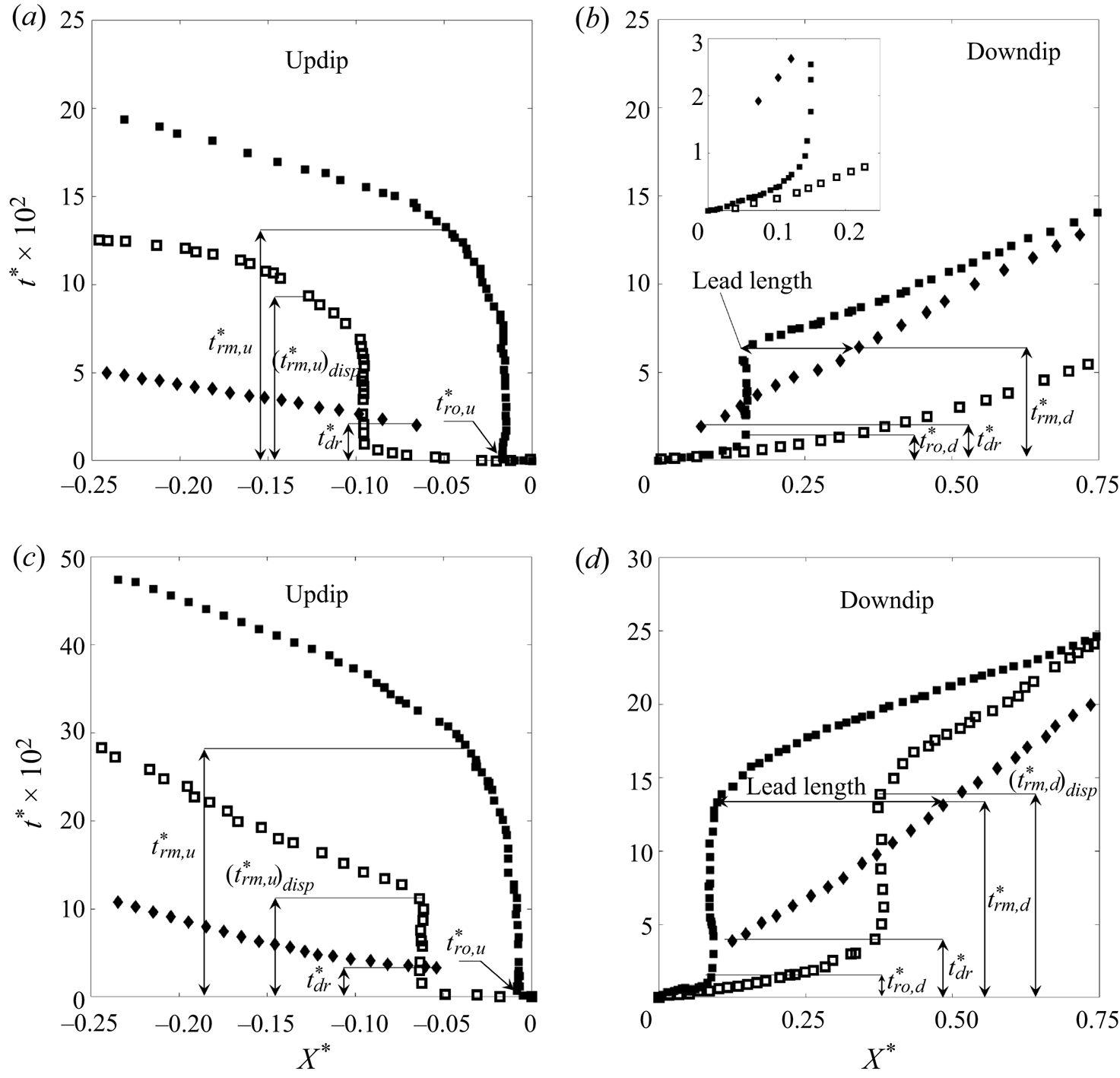
To characterize the behaviour of the gravity currents in the upper and lower layers, it is helpful to contrast the evolution of nose position, as shown in figure 5. Figure 5(a,b) correspond to  $g'_s = 20.1\pm 0.9\ \textrm {cm}\ \textrm {s}^{-2}$ (the same experiment shown in figure 3) and figure 5(c,d) correspond to
 $g'_s = 80.1\pm 0.9\ \textrm {cm}\ \textrm {s}^{-2}$. In both cases,
 $\theta =15^\circ$ and
 $Q_s = 1.01 \pm 0.02\ \textrm {cm}^{3}\ \textrm {s}^{-1}$ – see E50 and E58 of table 2. Although the primary gravity currents propagate along the sloping permeability jump, for the purposes of drawing an even dynamical comparison figure 5 resolves the flow of the primary (and secondary) gravity currents relative to the horizontal coordinate,
 $X$. In turn, the horizontal and vertical axes of figure 5 are respectively non-dimensionalized using the characteristic length and time scales defined in (2.2a,b). In the former case, we set
 $X^*= (X-X_s)/L$, such that
 $X^* = 0$ indicates the plume source location. Thus
 $X^*<0$ corresponds to the updip side (figure 5a,c) and
 $X^*>0$ corresponds to the downdip side (figure 5c,d). In all cases,
 $t^*=0$ indicates the time instant when the plume first strikes the permeability jump.
Time variation of the nose positions of the primary (squares) and secondary (diamonds) gravity currents for  $\theta =15^\circ$ and
 $Q_s = 1.01 \pm 0.02\ \textrm {cm}^{3}\ \textrm {s}^{-1}$. Closed and open squares correspond, respectively, to the bulk and dispersed interfaces: (a) Updip,
 $g'_s = 20.1\pm 0.9\ \textrm {cm}\ \textrm {s}^{-2}$; (b) downdip,
 $g'_s = 20.1\pm 0.9\ \textrm {cm}\ \textrm {s}^{-2}$; (c) updip,
 $g'_s = 80.1\pm 0.9\ \textrm {cm}\ \textrm {s}^{-2}$; and (d) downdip,
 $g'_s = 80.1\pm 0.9\ \textrm {cm}\ \textrm {s}^{-2}$. The variables
 $t_{ro,u}^*$,
 $t_{ro,d}^*$,
 $t_{rm,u}^*$,
 $t_{rm,d}^*$ and
 $t_{dr}^*$ are defined in text. The inset figure in panel (b) shows a close-up view of the early-time dynamics.

In addition to differentiating between the primary (squares) and secondary (diamonds) gravity currents, figure 5 also distinguishes between the noses associated with interfaces classified as bulk (solid squares) versus dispersed (open squares). The bulk interface noses of the primary gravity current reach their runout lengths at non-dimensional times  $t_{ro}^*$. Consistent with the above remarks,
 $t_{ro,d}^* > t_{ro,u}^*$, where ‘
 $u$’ and ‘
 $d$’ correspond, respectively, to updip and downdip. Along the downdip side, and for
 $t^* > t_{ro,d}^*$, the bulk interface nose of the primary gravity current remains fixed until such time as it gets remobilized by the secondary gravity current, a process described in more detail below. In contrast, and as observed for
 $g'_s = 20.1\pm 0.9\ \textrm {cm}\ \textrm {s}^{-2}$, the nose corresponding to the downdip dispersed interface continues to propagate with only a moderate deceleration until it reaches the sidewall boundary (figure 5b). Indeed, runout is realized with the dispersed interface only when (i) we examine the counterpart updip flow (figure 5a) or (ii) we increase the source reduced gravity e.g. from
 $g'_s = 20.1\pm 0.9\ \textrm {cm}\ \textrm {s}^{-2}$ (figure 5a,b) to
 $g'_s = 80.1\pm 0.9\ \textrm {cm}\ \textrm {s}^{-2}$ (figure 5c,d).
In the lower layer meanwhile, the draining fluid makes contact with the bottom boundary at  $t^*= t_{dr}^*$ and thereafter, propagates as a pair of oppositely-directed secondary gravity currents. At
 $t_{rm,d}^*$ (
 ${>}t_{dr}^*$), the secondary gravity current arising on the downdip side remobilizes the previously arrested primary gravity current. At the point of remobilization, figures 5(b) and 5(d) indicate that the secondary gravity current leads the primary gravity current by a horizontal distance that we shall refer to as the lead length. Corresponding to this lead length, we define a lead angle,
 $\varPhi$, in the manner suggested by figure 1(a). (Note that
 $\varPhi$ does not, in general, correspond to the angle made by the fluid draining into the lower layer.) On the updip side, and owing to the horizontal position of the nozzle, the secondary gravity current travels a shorter distance in
 $X^*$. Consequently, remobilization is delayed and arises only after the secondary gravity current has collided with the sidewall boundary leading to a steady accumulation of draining fluid and the vertical ascent of the first front through the lower layer. Note finally that the methodology for determining precisely the runout and remobilization times is summarized in Appendix C.
3.2. Primary versus secondary gravity currents, quantitative comparison
The lower layer depth,  $H_{lower}^*$, as characterized by its value measured directly below the nozzle and further non-dimensionalized by the total height,
 $H$, has a significant influence on the early-time flow dynamics of the primary gravity current, i.e. for
 $t^* \leqslant t_{{ro,d}}^*$. Consider, for example, figure 6(a), which considers five different values for the lower layer depth spanning the range
 $0.45 \leqslant H_{lower}^* \leqslant 0.70$. Runout is achieved for sufficiently large
 $H_{lower}^*$. Moreover, the time required for remobilization,
 $t_{rm,d}^*$, increases with the lower layer depth. When
 $H_{lower}^*$ is small, however, runout is bypassed, a process we refer to as runout override. Thus when
 $H_{lower}^* = 0.51$ or 0.45, the nose of the primary gravity current propagates, albeit unsteadily, without ever becoming arrested. In assessing whether runout will or will not occur, a comparison must be made between
 $t_{{ro,d}}^*$ and
 $t_{{dr}}^*$, only the latter of which depends (approximately linearly) on
 $H_{lower}^*$. The comparison in question appears in figure 6(b) where, for those experiments experiencing runout override, we suppose a value for
 $t^*_{ro,d}$ that is consistent with the companion data sets of figure 6(a). When
 $t_{{dr}}^* / t_{{ro,d}}^* \lesssim 1$ runout override is expected as indicated by the grey-shaded region in figure 6(b).
(a) Nose positions for the bulk interface of the primary gravity current. Time series corresponding to various lower layer depths,  $H^*_{lower}$, are compared. (b) The
 $t_{{dr}}^*/t_{{ro,d}}^*$ versus
 $H^*_{lower}$. The shaded region indicates the parametric range where we expect runout to be bypassed. The experiments correspond to
 $\theta =15^\circ$ and cases E49–E53 from table 2.

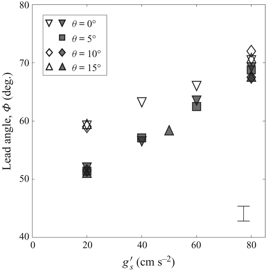
The lead angle,  $\varPhi$, is plotted versus
 $g^\prime _s$ for various permeability jump angles,
 $\theta$, in figure 7. The trend of the data is roughly linear with larger values of the lead angle occurring for smaller values of
 $Q_s$. Figure 7 suggests that the lead angle varies most strongly with
 $g^\prime _s$ followed by
 $Q_s$ and followed finally by
 $\theta$, the permeability jump angle exerting only a minor influence. Note also that the importance of the source volume flux is modulated by the source reduced gravity: whereas there is a significant disparity between the small versus large
 $Q_s$ data when
 $g'_s = 20.1 \pm 0.9\ \textrm {cm}\ \textrm {s}^{-2}$, this difference largely disappears for larger
 $g'_s$.
Variation of  $\varPhi$, as defined in figure 1(a), with
 $g'_s$ for different
 $\theta$. Open and closed symbols correspond to
 $Q_s = 0.51 \pm 0.02\ \textrm {cm}^{3}\ s ^{-1}$ and
 $1.01 \pm 0.02\ \textrm {cm}^3\ \textrm {s}^{-1}$, respectively. A representative error bar is shown in the lower right-hand corner.

For  $t^* > t_{rm,d}^*$, the front speed of the bulk fluid from the downdip primary gravity current is compared against the speed of the secondary gravity current in figure 8. The velocities of the primary and secondary gravity currents are both measured with respect to the horizontal and are both non-dimensionalized by the velocity factor
 $\beta$ defined in (2.4). When the lead angle is relatively small, e.g. when
 $Q_s = 1.01 \pm 0.02\ \textrm {cm}^3\ \textrm {s}^{-1}$ and
 $g'_s = 20.1\pm 0.9\ \textrm {cm}\ \textrm {s}^{-2}$, the primary and secondary gravity currents coexist and therefore exhibit approximately equal propagation speeds. When the lead angle is large, by contrast, the primary gravity current will, in general, only remobilize when the nose of the secondary gravity current is very close to, or has already collided with, the sidewall boundary. In such instances of non-coexistence, figure 8 exhibits a comparatively large range of primary gravity current speeds even as the (normalized) speeds of the secondary gravity currents remain nearly constant. In particular, there are situations (inset, downward-facing triangles) where the speeds of the primary and secondary gravity currents are approximately equal even though the gravity current pair is classified as being of non-coexistence type. Note also that the primary gravity current speed increases roughly linearly with
 $\theta$, an obvious reflection of the fact that larger permeability jump angles admit a more ready conversion of potential to kinetic energy. Additionally, and because the total height of our porous medium is fixed, large
 $\theta$ is associated with small
 $H_{R,{lower}}$ – see table 1. Correspondingly, fluid from the secondary gravity current has a relatively small vertical distance over which to advect before striking the permeability jump. As the fluid in question nears the permeability jump, it has a correspondingly larger influence on the bulk fluid of the primary gravity current for two reasons. First, the streamlines describing draining from the primary gravity current become deflected downdip. Second, with relatively less ambient fluid to displace from the lower layer, a greater fraction of the discharged plume fluid flows into the primary gravity current rather than into the lower layer. By both of these effects, we expect (and observe) the speed of the primary gravity current to increase with
 $\theta$.
Non-dimensional downdip front velocity,  $v^*$, versus
 $\theta$ for different source conditions. The closed symbols denote the primary gravity current and the open symbols denote the secondary gravity current. When the two gravity currents do not coexist, the marker symbols of both the primary and secondary gravity currents include a superimposed red cross. A representative error bar is shown in the bottom right-hand side corner.

4. Draining phenomenon and filling box flow
4.1. Characterization of the draining flow
To predict the speed of descent of the fluid draining through the lower layer, it is necessary to define an average draining length as
 \begin{equation} \bar{l}(t) = \frac{1}{x_{N_d}(t)-x_{N_u}(t)} \int_{{-}x_{N_u}(t)}^{x_{N_d}(t)} l(\tilde{x},t)\,\mathrm{d}\tilde{x}, \end{equation}
where  $x_{N_u}$ and
 $x_{N_d}$ are, respectively, the up- and downdip nose positions of the bulk interface and
 $l$ is the vertical distance traversed by the draining fluid as measured relative to the permeability jump. The time variation of the non-dimensional average drain length,
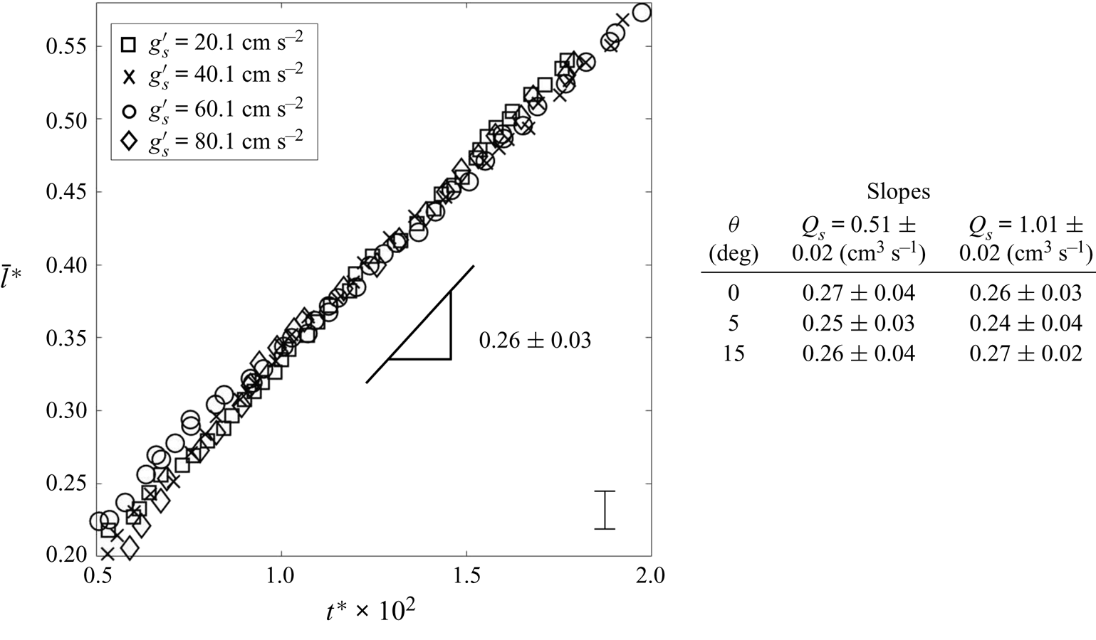
 $\bar {l}^*\equiv \bar {l}/H$, is shown in figure 9 for a variety of source conditions. Consistent with figure 6(b) and the study by Acton, Huppert & Worster (Reference Acton, Huppert and Worster2001),
 $\bar {l}^*$ shows a linear increase with time, except at very early times (not shown in figure 9).
Evolution of the average draining length,  $\bar {l}^*$, with
 ${t^*}$ for various
 $g'_s$ with
 $\theta = 0^\circ$ and
 $Q_s = 1.01 \pm 0.02\ \textrm {cm}^{3}\ \textrm {s}^{-1}$. The average slope of the data (as measured over the interval
 $0.5 \leqslant t^* (\times 10^2) \leqslant 2$) is reported. The adjoining table indicates the slope values measured for other combinations of
 $\theta$ and
 $Q_s$.

4.2. Simultaneous versus sequential filling
In § 2.3, we suggested that the filling of the two-layer porous medium could be classified as simultaneous or sequential depending on whether or not the upper and lower layers fill concurrently. Drawing such a distinction is important for the following reason: our analysis has assumed buoyancy and viscosity as the dominant dynamical balance; however, there are other scenarios (Golding et al. Reference Golding, Neufeld, Hesse and Huppert2011; Burnside & Naylor Reference Burnside and Naylor2014; Krevor et al. Reference Krevor, Blunt, Benson, Pentland, Reynolds, Al-Menhali and Niu2015) where capillarity is expected to play a non-subordinate role. In such cases, residual trapping of the injectate is expected to be important. The amount of trapping is found to vary according to whether the intruding flow is primarily horizontal versus vertical (Adebayo, Barri & Kamal Reference Adebayo, Barri and Kamal2017). Because sequential and simultaneous filling are associated with different proportions of horizontal versus vertical flow, the details of the filling mode will, for this more general case of intermediate Bond number, influence the degree of residual trapping.
A rigorous way of distinguishing sequential versus simultaneous filling is discussed in Appendix D. On this basis, an assessment can be made of the filling mode for each of the experiments performed. A summary of results, pertinent to  $Q_s = 1.01\pm 0.02\ \textrm {cm}^3\ \textrm {s}^{-1}$, is presented in figure 10 (see also table 2 of Appendix A). The horizontal axes of figure 10 indicate the nozzle position and source reduced gravity, whereas the vertical axis indicates the permeability jump angle. The red and blue symbols respectively indicate cases of simultaneous and sequential filling. The grey region indicates a transition region from one filling mode to the other.
Downdip filling mode as a function of nozzle position, source reduced gravity and permeability jump angle. The red symbols indicate simultaneous filling, while the blue symbols indicate sequential filling. The grey region separating the red and blue symbols signifies a transition region.

When the source reduced gravity is low or moderate, such as for  $g^\prime _s = 20.1\pm 0.9\ \textrm {cm}\ \textrm {s}^{-2}$, the primary gravity current experiences significant dispersion and the nose of the dispersed fluid collides with the sidewall boundary well before the nose of the secondary gravity current – cf. figure 5(b). Thus the upper layer begins to fill well before the secondary layer is filled with contaminated fluid. Generalizing, simultaneous filling is anticipated for small
 $g'_s$ irrespective of the nozzle position or permeability jump angle. By contrast, the tendency for sequential filling is greater when the source reduced gravity is comparatively large implying (i) shorter runout lengths for the bulk fluid, and, (ii) the possibility of runout for the dispersed fluid – see figure 5(d). Note, however, that sequential filing is realized in actual fact only when the nozzle is shifted updip. Regarding the influence of
 $\theta$, figure 10 indicates that the filling mode changes as a result of adjusting
 $\theta$ only in the following instance:
 $\theta = 0^\circ$ to
 $\theta = 5^\circ$ for
 $g'_s = 80\ \textrm {cm}\ \textrm {s}^{-2}$ and the nozzle located at the centre of the tank. Figure 10 makes clear the fact that simultaneous filling occurs for small
 $g'_s$, large
 $\theta$ and downdip-shifted nozzles. By contrast, sequential filling is favoured for large
 $g'_s$, small
 $\theta$ and a nozzle shifted updip.
The surface plots of figure 11 show the normalized filling box time,  $\hat {t}_{{fb}}$, as a function of
 $\theta$ and
 $X_s^*$ where both large and small values of
 $g'_s$ are considered. We define the filling box time as the time taken for the first front propagating through the upper layer to reach a vertical height corresponding to the approximate upper boundary of the porous medium, i.e.
 $Z^* = 0.99$. Complications arise because the first front is not always horizontal; rather, the upper layer may fill faster in the vicinity of the sidewall boundaries and more slowly in the neighbourhood of the plume. This phenomenon is more prevalent for small
 $g'_s$ and persists even in the limit of large first front elevations – see figure 16(a,c). For these reasons, we define in figure 11 the two following filling box times: (i)
 $\hat {t}_{{fb}\downarrow }$ from figure 11(a) represents a lower-bound estimate to the filling box time that is defined as the time when any portion of the first front (whether to the left or right of the descending plume) first reaches the elevation
 $Z^* = 0.99$; (ii)
 $\hat {t}_{{fb}\uparrow }$ from figure 11(b) represents an upper-bound estimate to the filling box time that is defined as the time when the entirety of the first front first has reached
 $Z^* = 0.99$. The filling box times exhibited in figure 11(a,b) exhibit minor variations with
 $\theta$ and
 $X^*_s$; however, a more interesting variety appears when considering the influence of the source reduced gravity. To wit,
 $\hat {t}_{{fb}\downarrow } (g'_s = 20.1\pm 0.9\ \mbox {cm}\ \textrm {s}^{-2}) < \hat {t}_{{fb}\downarrow } (g'_s = 80.1\pm 0.9\ \mbox {cm}\ \textrm {s}^{-2})$ but
 $\hat {t}_{{fb}\uparrow } (g'_s = 20.1\pm 0.9\ \mbox {cm}\ \textrm {s}^{-2}) > \hat {t}_{{fb}\uparrow } (g'_s = 80.1\pm 0.9\ \mbox {cm}\ \textrm {s}^{-2})$. When
 $g'_s = 20.1\pm 0.9\ \textrm {cm}\ \textrm {s}^{-2}$, the filling mode is always simultaneous and flows, particularly of the primary gravity currents, are characterized by ample dispersion. As a result, and although the upper layer fills relatively quickly with contaminated fluid, it does so non-uniformly. In other words, an abundance of contaminated fluid accumulates along the right sidewall boundary because the potential energy penalty associated with a significantly-deflected first front is small. Thus, it takes relatively little time for the first front to first reach
 $Z^* = 0.99$ but appreciably more time for the entirety of the first front to reach this elevation. The situation for
 $g'_s = 80.1\pm 0.9\ \textrm {cm}\ \textrm {s}^{-2}$ is rather different. Here, less dispersion arises and, according to figure 10, the filling mode may be either simultaneous or sequential. In either case, the slope of the first front is smaller than when
 $g'_s = 20.1\pm 0.9\ \textrm {cm}\ \textrm {s}^{-2}$. Correspondingly, the gap between
 $\hat {t}_{{fb}\downarrow }$ and
 $\hat {t}_{{fb}\uparrow }$ is smaller by comparison.
Lower- (a) and upper- (b) bound estimates of the non-dimensional filling box time plotted as a function of the permeability jump angle,  $\theta$, and the source position,
 $X_s^*$. Two values for the source reduced gravity,
 $g'_s$, are considered where, in either case,
 $Q_s = 1.01 \pm 0.02\ \textrm {cm}^3\ \textrm {s}^{-1}$. To show the lower surface more clearly, the upper surface is purposely made semi-transparent in both plots.

4.3. Plume deflection
In § 1, reference was made to plumes that become deflected as a result of a background mean flow (Weaver & Wilson Reference Weaver and Wilson2000; Van Stempvoort et al. Reference Van Stempvoort, Roy, Grabuski, Brown, Bickerton and Sverko2013) and/or stratigraphic steering (Morgan et al. Reference Morgan, Kent, Seitz and Novak2008; Kamath et al. Reference Kamath, Connor, McHugh, Nemir, Le and Ryan2012). Motivated by recent observations of turbulent, non-porous media plumes made by Akhter & Kaye (Reference Akhter and Kaye2020), we now explore a further possibility, namely that a plume becomes deflected as a result of a hydrostatic pressure imbalance associated with fluid discharge from the selfsame plume.
When  $\theta = 0^\circ$ and the nozzle is centrally located, there exists, not surprisingly, a flow symmetry about
 $X_s^* = 0.5$ – cf. figure 5(a–c) of the paper by Sahu & Flynn (Reference Sahu and Flynn2017). This symmetry can be broken by adjusting
 $\theta$ and/or the location of the plume nozzle. Figure 12(a–c) shows experimental snapshot images where
 $\theta = 15^\circ$ and the nozzle is situated at
 $X_s^*=0.25, 0.5$ and 0.75, respectively.
False-colour snapshot images showing the deflection of the plume when the source is located (a) updip at  $X_s^*=0.25$, (b) centrally at
 $X_s^*=0.5$ and (c) downdip at
 $X_s^*=0.75$. The red arrows indicate the magnitude of the plume deflection. The deflection angle,
 $\psi$, is defined in (c). Experimental parameters are as follows:
 $\theta = 15^\circ$;
 $g^\prime _s= 20.1\pm 0.9\ \textrm {cm}\ \textrm {s}^{-2}$; and
 $Q_s = 1.01 \pm 0.02\ \textrm {cm}^{3}\ \textrm {s}^{-1}$.

In figure 12(a–c), the nozzle is respectively shifted up- to downdip, but there is an opposite trend when considering the plume deflection. By contrast with the case of a flat permeability jump, figure 12(b) confirms that an (updip) deflection of the plume is possible even when the nozzle is centrally located. When the plume is not centrally located, figure 12(a,c) confirm that the deflection direction is away from the closer sidewall boundary. Interestingly, precisely the opposite trend was noted in the recent filling box experiments of Akhter & Kaye (Reference Akhter and Kaye2020), who considered turbulent non-porous media plumes and observed that the deflection direction was towards, not away from, this adjacent sidewall boundary. In summarizing the explanation by Akhter & Kaye (Reference Akhter and Kaye2020) of their observations, reference is made to the short and long sides, which respectively indicate the sides of the experimental tank having the shorter versus longer horizontal distances from the descending plume to a sidewall boundary. Regarding the discharged plume fluid that accumulated along the bottom of their box, Akhter & Kaye (Reference Akhter and Kaye2020) noted that the depth of this layer was larger on the short side versus the long side. They surmised that the resulting hydrostatic pressure imbalance led to a net circulation inside their filling box: at depth, dense fluid flowed from the short to the long side resulting in an oppositely-directed return flow of ambient fluid close to the plume source. Because our experiments are characterized by upper and lower layers, they admit a greater variety in terms of return flow pathways. Moreover, any overall circulation that develops within our filling box is expected to be comparatively weaker than in the experiments of Akhter & Kaye (Reference Akhter and Kaye2020) owing to the retarding influence of the porous medium. Correspondingly, and when the plume is shifted off-centre, we observe a deflection only in the direction of the long side. In the process, there arises the interesting scenario illustrated in figure 12(c) (and also figure 12b) whereby the plume bends towards, rather than away from, the (lower) layer of smaller permeability. This observation runs contrary to the pattern of streamline deflection that is associated with flow focusing whereby the flow is attracted to lenses of higher permeability – see e.g. figure 3.11 A of the book by Phillips (Reference Phillips1991).
Seeking to quantify the effects illustrated in figure 12, we define a plume deflection angle,  $\psi$, in the manner suggested by figure 12(c). When the plume deflects updip (downdip),
 $\psi$ assumes a negative (positive) value. The time variation of
 $\psi$ for the experiment illustrated in figure 12(c), is exhibited in figure 13(a). Initially, the plume shows no deflection; at
 $\hat {t}= 0.04$ the plume starts to deflect updip and there is a corresponding increase in the magnitude of
 $\psi$. For
 $\hat {t} \gtrsim 0.2$,
 $\psi$ approaches its asymptotic value corresponding, in magnitude, to a maximum deflection angle,
 $\psi _{max}$. In figure 13(b),
 $\psi _{max}$ values are plotted versus
 $\theta$. In this same plot, comparisons are made against two different source reduced gravities corresponding to
 $g^\prime _s= 20.1\pm 0.9$ (closed symbols) and
 $80.1\pm 0.9\ \textrm {cm}\ \textrm {s}^{-2}$ (open symbols). It is observed that the magnitude of
 $\psi _{max}$ typically increases with
 $\theta$. Additionally, when the nozzle is shifted updip, the plume deflects downdip such that
 $\psi _{max} > 0^\circ$. By contrast,
 $\psi _{max} < 0^\circ$ when the nozzle is located at the centre of the box or is shifted downdip. For fixed source conditions, this latter case is associated with the largest values for
 $|\psi _{max}|$. When the source conditions are not fixed,
 $\psi _{max}$ depends strongly on the source reduced gravity: for
 $g^\prime _s= 80.1\pm 0.9\ \textrm {cm}\ \textrm {s}^{-2}$, the magnitude of plume deflection is significantly less than in the
 $g'_s = 20.1 \pm 0.9\ \textrm {cm}\ \textrm {s}^{-2}$ case. Plumes containing comparatively dense fluid are more difficult to deflect and tend, therefore, to assume more of a vertical trajectory.
(a) Variation of the plume deflection angle,  $\psi$, as a function of time for the experiment illustrated in figure 12(c). (b) The magnitude-maximum deflection angle,
 $\psi _{max}$, plotted as a function of permeability jump angle and nozzle location. Closed and open symbols respectively show
 $g^\prime _s= 20.1\pm 0.9\ \textrm {cm}\ \textrm {s}^{-2}$ and
 $80.1\pm 0.9\ \textrm {cm}\ \textrm {s}^{-2}$. In (b), symbols are connected by lines only for the sake of identifying more clearly trends within the data; the lines do not suggest a curve fit. Representative error bars are shown in the lower right-hand corner of each plot.

The deflection of the plume is expected to have a relatively minor impact on the overall entrainment of ambient fluid. When the plume deflects, (i) the path length increases, but, (ii) the plume centreline velocity decreases. Because the former and latter effects respectively serve to increase and decrease the rate of entrainment, we anticipate, by analogy with angled turbulent plumes (Lee & Chu Reference Lee and Chu2003), the net contribution to be even. On the other hand, once the plume becomes deflected, the balance of discharged plume fluid flowing up- versus downdip must adjust, which may, in turn, impact the subsequent rate of filling of the upper and lower layers. Such considerations are especially relevant in the context of figure 12(a,c). In the former figure, the plume deflects downdip suggesting a more rapid filling of the upper layer in the neighbourhood of the right sidewall boundary and a smaller value for  $\hat {t}_{{fb}\downarrow }$. Precisely the opposite trend is expected in figure 12(c) where the plume deflects updip, which has the effect of (i) directing more dense fluid towards the left sidewall boundary, (ii) reducing the left-to-right difference in the elevation of the first front, and (iii) increasing
 $\hat {t}_{{fb}\downarrow }$.
5. Discussion
To this point, we have discussed three ostensibly distinct aspects of porous media filling box flows namely (i) the runout and subsequent remobilization of the primary gravity currents, (ii) the filling mode, be this simultaneous or sequential, and (iii) the deflection of the descending plume. In fact, (i), (ii) and (iii) are all tightly interconnected. For example, the stasis characterizing runout is interrupted only when sufficient dense fluid has drained into the lower layer and, for example, the lead angle,  $\varPhi$, defined by figure 7, is exceeded. Thus the initial filling of the lower layer has a direct impact on the process of remobilization and, more generally, the gravity current flows observed along the permeability jump. On the other hand, it is the competition between the primary and secondary gravity currents that dictates whether the first contaminated fluid to reach the downdip sidewall boundary does so along the permeability jump or along the bottom of the box. In this way, the motion of the gravity currents (complicated by the process of dispersion in the upper layer) determines whether or not the upper layer begins to fill before the filling process is complete in the lower layer. Finally, and as highlighted most especially by figure 12, plume deflection arises precisely because of left-to-right asymmetries in the manner in which the upper layer fills with contaminated fluid. On the other hand, once the plume is deflected, the proportion of discharged plume fluid directed up- versus downdip will adjust. In turn, such an adjustment increases the volume of dense fluid supplied to the updip gravity current and impacts the subsequent evolution of the filling process.
As the above explanation makes clear, no single aspect of the filling box dynamics can be categorized comprehensively without considering the impact of the other two. Somewhat after-the-fact, this rationalizes why the present analysis is so much more involved than that summarized by Bharath et al. (Reference Bharath, Sahu and Flynn2020). In that study, the lower layer was effectively considered infinitely deep such that the dynamical phenomena of remobilization, layer filling and plume deflection became moot. On the other hand, even the more involved analysis considered in the present work examines only two layers whereas porous media of the type modelled numerically in the hydrogen storage study of Feldmann et al. (Reference Feldmann, Hagemann, Ganzer and Panfilov2016) contain many more strata, each of different permeability and thickness. Generalizing our results and the interconnections summarized above to this more complicated geometrical description remains a challenge to be conquered in future work.
6. Summary and conclusions
We have performed an experimental investigation of buoyancy-driven flows in a two-layered porous medium where the layers are separated by an inclined permeability jump. Throughout, the lower layer had a permeability that was  $\frac {1}{9}\mathrm {th}$ the permeability of the upper layer. Experiments were conducted under ambient conditions and entailed the injection of dense saltwater into the saturated porous medium leading to the formation of a vertically-descending plume plus gravity currents that propagated along the permeability jump and also along the bottom boundary of the experimental domain. Flows were visualized by the addition of a small amount of dye to the source fluid. In turn, we studied the impact of altering the permeability jump angle, the plume source horizontal location, the source volume flow rate and the source reduced gravity.
In contrast to previous studies (Goda & Sato Reference Goda and Sato2011; Bharath et al. Reference Bharath, Sahu and Flynn2020) that have assumed upper and lower layers of great depth, a novel contribution of the present work is to specifically consider the effect of impermeable boundaries, both lateral and basal. As such, we focus on the processes of upper- and lower-layer filling. In the former case, filling follows from the up- and downdip flow of the primary gravity currents followed by the vertical advection of the first front. In the latter case, filling is related to the advection of the secondary gravity currents that propagate along the base of the lower layer. Added to this advection is the contribution of leakage through the permeability jump, which leads to convection over a broad area. In quantifying the dynamics of layer filling, time series images were constructed to analyse the evolution of flow fronts in both the upper and lower layers – see figure 4. An additional benefit of such figures lies in their revelation of primary gravity current dispersion (Sahu & Neufeld Reference Sahu and Neufeld2020). Correspondingly, and when describing the primary gravity current, we differentiate between the bulk versus the dispersed phases. Except when the lower layer was relatively shallow, the former phase achieved runout, a state of (temporary) stasis wherein the plume inflow is balanced by basal draining. By contrast, runout was only observed for the dispersed phase of the primary gravity current when the plume source density was sufficiently large. Predictions of the runout distance have been made in previous studies; they were characterized by a permeability jump that is flat (Goda & Sato Reference Goda and Sato2011; Sahu & Flynn Reference Sahu and Flynn2017) or sloping (Bharath et al. Reference Bharath, Sahu and Flynn2020). A fundamentally new component of our analysis is to characterize the remobilization of the primary gravity currents that arises some time after these primary gravity currents are surpassed by their secondary gravity current counterparts. We characterize, at the time of remobilization, the separation distance between the primary and secondary gravity currents by making reference to a lead angle,  $\varPhi$ – see figure 1(a). From figure 7, we note that
 $\varPhi$ varies approximately linearly with the source reduced gravity but is uninfluenced by the permeability jump angle.
Whatever the particular details of runout and remobilization, comparisons can be drawn between the motion of the primary and secondary gravity currents – see e.g. figures 5 and 6. On the basis of this comparison, we find that when the primary and secondary gravity currents coexist, they travel at nearly equal velocities that are, in turn, nearly independent of the permeability jump angle – see figure 8. The jump angle plays a more important dynamical role for the case of non-coexistence, i.e. it exerts a significant influence on the speed of the remobilized primary gravity current.
In categorizing the nature of the filling in our layered porous medium, we distinguish between modes described as simultaneous versus sequential. The differences between one and the other filling regime are analysed by considering an example of each – see e.g. figure 16. From the analysis of figure 10, it is observed that simultaneous filling is favoured when the source reduced gravity is relatively small and the nozzle is located close to the downdip sidewall boundary. The question of whether sequential versus simultaneous filling occurs is important when considering the dynamics of the lower layer in particular. In sequential filling, most of the filling of the lower layer is by the horizontal advection of the secondary gravity current. By contrast, and for simultaneous filling, proportionally more of the lower layer filling is by basal draining from the overlying primary gravity current. In the abstract, and for real geological flows, drawing a distinction between simultaneous versus sequential filling is important: as highlighted in § 4.2, either should be associated with a different degree of residual trapping, this for the case (not studied here) where capillary effects make a non-trivial contribution to the flow dynamics.
Whichever the filling mode, the experimental domain must at some point become effectively completely filled with contaminated fluid, defined as fluid having a density larger than that of the ambient fluid that fills the box at the initial instant. The time for this complete filling is defined as the filling box time,  $\hat {t}_{fb}$ i.e. the time required for the first front rising through the upper layer to very nearly reach the level of the plume source. In fact, and for the flows examined here, the inclination of the first front makes defining
 $\hat {t}_{fb}$ unambiguously somewhat challenging. Rather, we consider in figure 11 lower (
 $\hat {t}_{{fb}\downarrow }$) and upper (
 $\hat {t}_{{fb}\uparrow }$) bound estimates to the filling box time. Whereas
 $\hat {t}_{{fb}\downarrow }$ and
 $\hat {t}_{{fb}\uparrow }$ vary little with the permeability jump angle and the horizontal position of the plume source, we find that dispersion causes the difference
 $\hat {t}_{{fb}\uparrow }-\hat {t}_{{fb}\downarrow }$ to be much larger when the source reduced gravity is comparatively small.
In the final component of our analysis, we investigated the trajectory of the descending plume and the manner in which this varies with time owing to the filling of the upper layer. The plume may deflect either up- or downdip depending on the source reduced gravity and the nozzle location relative to the sidewall boundary. In turn, the time variation of the plume deflection angle,  $\psi$, and the magnitude-maximum deflection angle,
 $\psi _{max}$, are characterized in figure 13.
The observations made in this experimental study help to address some of the key uncertainties arising from leakage across a permeability jump. In contrast to numerous previous studies for which the layer defined as our lower layer is either thin (Pritchard et al. Reference Pritchard, Woods and Hogg2001; Farcas & Woods Reference Farcas and Woods2009; Woods & Farcas Reference Woods and Farcas2009) or infinite (Goda & Sato Reference Goda and Sato2011; Bharath et al. Reference Bharath, Sahu and Flynn2020), we consider instead a lower layer of intermediate depth. To this end, we find that the depth of the lower layer is important e.g. in dictating whether or not a state of intermediate runout is achieved – see figure 6. The lower layer depth also influences the manner in which the lower layer fills, i.e. whether by the advection of the secondary gravity current or else by the process of basal draining defined above. In studying the intermediate- and late-time dynamics, we find also that the flow propagation is effected by the sidewall boundaries which ultimately impede up- and downdip flow propagation and thereby act as a localized trap (Buschkuehle Reference Buschkuehle2005). The filling modes identified in this study help to predict the time required to fill these traps and, by extension, the adjoining high versus low permeability layers.
Acknowledgements
The authors acknowledge the kind assistance provided by the Alberta Geological Survey, who supplied the authors with several relevant reports. The authors are grateful to Professor B.R. Sutherland who graciously offered the required space and facilities in his Environmental and Industrial Fluids Laboratory to conduct all our experiments. The authors also are thankful to Dr-Ing. B. Hagemann for providing relevant information on his published work.
Funding
The current research is supported by NSERC (Discovery Grant and RTI programmes).
Declaration of interests
The authors report no conflict of interest.
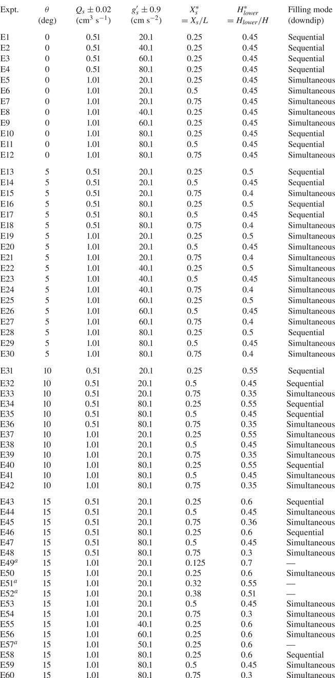
Appendix A. List of experiments
A summary of the laboratory experiments performed as part of this study is given in tabular form below.
List of laboratory experiments.

Appendix B. Dye calibration procedure
The amount of dye to be mixed into the source fluid was determined from the methodology of Dong & Selvadurai (Reference Dong and Selvadurai2006). Accordingly, correlations between the dye concentration and normalized pixel intensity were obtained then plotted as in figure 14. Two separate calibration curves, one corresponding to the upper layer and other to the lower layer, were generated. Such a duplication is necessary because the two layers are composed of glass beads of different diameters. As such, the layers do not transmit the same fraction of (background) light with the lower layer appearing darker than the upper layer, cf. figure 1(b). Calibration curves such as those shown in figure 14 were obtained by completely filling the heterogeneous porous medium with (fresh) water of known dye concentration then capturing images using a Canon Rebel EOS T2i 18.0 PM camera. Multiple images were collected and the dye concentration varied from 0 to  $0.3\ \textrm {g}\ \textrm {l}^{-1}$. Images were then processed using Matlab to obtain the calibration curves. We observe from figure 14 that, owing to the smaller permeability of the lower layer, the pixel intensity saturates comparatively quickly. Therefore, the dye concentration used in all of our experiments was set by the lower layer calibration curve, which demanded, in turn, that we limit the dye concentration to
 $0.15\ \textrm {g}\ \textrm {l}^{-1}$.
Dye calibration curves.

Appendix C. Method for determining  $t_{ro}^*$ and $t_{rm}^*$


To demonstrate the method for identifying the time to runout and the time to remobilization, we consider the downdip propagation of the primary gravity current for the case illustrated in figure 5(a,b). The evolution of the nose is divided into three time periods, which are curve-fitted by polynomial curves C1, C2 and C3 in figure 15. The point of intersection of C1 with C2 specifies the time to runout. Conversely, the point of intersection of C2 and C3 gives the time for remobilization.
Method to determine, for the primary gravity currents, the time to runout,  $t_{ro}^*$, and the time for remobilization,
 $t_{rm}^*$ . Panels (a) and (b) respectively consider the up- and downdip sides. C1, C2 and C3 indicate curve fits for data points corresponding to different stages of motion, i.e. initial propagation, runout and remobilization. C1 is a third-degree polynomial, whereas for C2 and C3 the fitted curve is a first-degree polynomial.

Appendix D. Method for identifying simultaneous versus sequential filling
Consider figure 16, whose panels (a) and (b) show snapshot images of experiments E19 and E28, respectively. In both cases  $\theta = 5^\circ$,
 $Q_s = 1.01 \pm 0.02\ \textrm {cm}^3\ \textrm {s}^{-1}$ and the plume nozzle is located at
 $X_s^*=0.25$. However, in figure 16(a),
 $g^\prime _s=20.1\pm 0.9\ \textrm {cm}\ \textrm {s}^{-2}$ and the filling mode is simultaneous. By contrast, in figure 16(b),
 $g^\prime _s=80.1\pm 0.9\ \textrm {cm}\ \textrm {s}^{-2}$ and the filling mode is sequential. In making these assessments, reference is made to the surface plots of figure 16(c,d). These surface plots are generated by stacking in the vertical coordinate,
 $Z^*= Z/H$, contour lines derived from a horizontal time series analysis that follows from the procedure outlined in § 2.3. The surfaces therefore indicate, for prescribed
 $X^*$ and
 $Z^*$, the moment in time when the pixel intensity first obtains a non-trivial value. This is, of course, the same instant when discharged plume/contaminated fluid is first detected at the location in question. The surfaces span the entire depth of the porous medium i.e. they draw data from the upper and lower layers. However, the surfaces pertain only to the downdip side of the nozzle. Analogue surface plots corresponding to the updip side are straightforward to construct but are not shown here. For illustrative purposes, it is also helpful to consider the shape of some of the contour lines that constitute the surfaces of figure 16(c,d). To this end, figure 16(e,f) correspond to figure 16(c,d), respectively. In both line plots, data points falling on contour lines corresponding to
 $0.005 \leqslant Z^* \leqslant 0.3$ lie completely within the lower layer. Data points falling on the contour line labelled (
 $Z^*=$) 0.4 span both the upper and lower layers. Finally, data points falling on the contour line labelled (
 $Z^*=$) 0.99 lie completely within the upper layer. In either of figure 16(e,f), and except for the curve labelled (
 $Z^*=$) 0.99, the general trend of each curve is increasing. However, and as we explain below, it is the rate of increase between those curves labelled e.g. as (
 $Z^*=$) 0.005 and (
 $Z^*=$) 0.4 that is especially significant when distinguishing between simultaneous versus sequential filling.
False-colour snapshot images in panel (a,b), surface plots in panel (c,d) and line plots in panel (e,f), for simultaneous (left panels,  $g'_s = 20.1 \pm 0.9\ \textrm {cm}\ \textrm {s}^{-2}$) and sequential filling (right panels,
 $g'_s = 80.1 \pm 0.9\ \textrm {cm}\ \textrm {s}^{-2}$). The vertical locations of the curves, i.e.
 $Z^*= 0.005$, 0.25, 0.3, 0.4 and 0.99, exhibited in (e,f) are indicated in the snapshot images (a,b) by the dashed horizontal lines. Additionally, the arrows in (e,f) point in the direction of increasing
 $Z^*$. In (c,d), the position of the permeability jump is indicated by the vertical plane (green). Here
 $\theta = 5^\circ$ and
 $Q_s = 1.01 \pm 0.02\ \textrm {cm}^3\ \textrm {s}^{-1}$.

When  $g^\prime _s= 20.1\pm 0.9\ \textrm {cm}\ \textrm {s}^{-2}$, the snapshot of figure 16(a) confirms that, on the downdip side, the upper layer begins to fill with dispersed fluid before the lower layer. This behaviour is more clearly illustrated in figure 16(c), whose surface exhibits a vertical dip (highlighted by the vertical arrow) just below the permeability jump and for sufficiently large
 $X^*$. The dip reflects the fact that dispersed fluid from the primary gravity current reaches the sidewall boundary at relatively early times. Thereafter, the dispersed fluid in question either drains (slowly) into the lower layer or else accumulates in a steadily thickening layer at the base of the upper layer. By contrast, the secondary gravity current forms later and so the base of the lower layer in the neighbourhood of
 $X^* = 0.75$ begins filling with contaminated fluid only after the upper layer is, in effect, completely filled. This latter conclusion is supported by figure 16(e). Contrasting the curves labelled 0.005 and 0.99 in the limit of large
 $X^*$, we note that contaminated fluid is observed in the neighbourhood of the top of the box at an earlier time than contaminated fluid is noted in the neighbourhood of the bottom of the box. For those pixels along
 $Z^*=0.005$, filling is associated with the horizontal advection of the secondary gravity current, thus the nearly linear increase of the curve labelled 0.005 in figure 16(e). Such linear behaviour disappears when
 $Z^*=0.25$ or
 $0.3$, because at these larger elevations, the intrusion of contaminated fluid stems from the combination of the secondary gravity current and basal draining from the overlying primary gravity current. In contrast to figure 16(a), figure 16(b) considers
 $g^\prime _s= 80.1\pm 0.9\ \textrm {cm}\ \textrm {s}^{-2}$ and shows an example of sequential filling. The right-hand side edge of the surface from figure 16(d) corresponds to
 $X^* = 0.75$ and shows a monotone (and nearly linear) variation as highlighted by the long black arrow. In like fashion, the curves from figure 16(f) show, for sufficiently large
 $X^*$, a progressive increase from small to intermediate to large values of
 $Z^*$.