


Understanding how politics affects the allocation of public resources is central to the study of political institutions. Of particular concern in American politics is whether and how congressional majorities (e.g., Bickers and Stein Reference Bickers and Stein2000; Lazarus and Steigerwalt Reference Lazarus and Steigerwalt2009; Levitt and Snyder Reference Levitt and Snyder1995) and presidents (e.g., Berry, Burden, and Howell Reference Berry, Burden and Howell2010; Reeves Reference Reeves2011) influence the geographic allocation of federal expenditures. One fruitful approach to understanding these influences has been to examine over-time variation in spending for geographic areas as partisan control of the legislature, presidency, and individual seats changes. On the basis of this type of design, previous work finds that states with two senators in the majority receive about 2% more in spending than do other states (Albouy Reference Albouy2009), whereas House districts represented by members of the president's party receive about 4% more in discretionary federal spending than other districts (Berry, Burden, and Howell Reference Berry, Burden and Howell2010).Footnote 1 A key theoretical question is how to interpret these findings. Are presidents and congressional parties rewarding supportive legislators, or are they rewarding supportive voters?
Answering this question has important implications for understanding what is at stake in congressional and presidential elections for both voters and legislators. It also illuminates the role of parties in facilitating interbranch coordination. Does it matter for places that support a Democratic president that they are also represented by a Democratic legislator, or is it the president's partisanship that is far more important? Put differently, are Democratic presidents good for Detroit because of the president's likely strong showing there or because Democrats also tend to hold House seats in the city?
We argue that these goals—to reward either same-party voters or same-party legislators—are not usually in conflict; places with many Democratic (Republican) voters tend to both elect Democratic (Republican) House members and support the Democratic (Republican) presidential candidate. However, because the vast majority of federal spending is programmatic and not readily amenable to geographic targeting to districts represented by particular legislators, it is generally far easier—and therefore more efficient—to pursue policies that benefit like-minded voters than to target individual House districts. Thus, the former pattern will tend to dominate the latter. For presidents, personal ideological and electoral considerations explain preferences for policies that favor same-party voters, as well as those in the swing states necessary to build an Electoral College majority. At the same time, presidents have important reasons to support same-party legislators, but given the difficulty of achieving this goal, they should act on it only in a targeted manner by directing particularistic spending, which makes up a small fraction of overall expenditures, to members of their party who are electorally vulnerable. The House majority operates under similar constraints, but because legislation is subject to majority-party review, the majority is more likely to supplement policies targeted at voters and electorally vulnerable party members with those targeted at majority-party districts.
In distinguishing between accounts based on legislator and voter partisanship, we identify an important research design concern in prior work: variation in the partisanship of locally elected House members is systematically correlated with voter preferences, both of which may cause differences in government spending. Analysts therefore need to take steps to separate the effects of the partisanship of a district's elected officials from the partisan disposition of the mass electorate to avoid misattributing the source of variation in spending.Footnote 2 In light of these concerns, we undertake two new types of analysis. Our first strategy replicates prior pooled cross-sectional studies while also accounting for the partisan composition of a district's electorate. Our second strategy holds fixed the partisan representation of districts by focusing on the same individual members who serve in multiple institutional environments—either in both the House majority and minority or with a same- and opposing-party president.
We use these research designs to investigate three broad categories of important theoretical questions. First, we examine how the strategic incentives and powers of the president affect the allocation of federal funds. We test whether presidents are associated with additional resources for same-party House members (either overall or among vulnerable incumbents), districts with more same-party voters, or the swing states necessary to secure an Electoral College majority. Second, we explore how the majority party in the House uses its influence. We assess whether the House majority is associated with additional spending in districts held by its members (either overall or among vulnerable incumbents), as well as in places with more supportive electorates. Finally we examine the individual-level factors—seniority, electoral vulnerability, and key positions in party and committee leadership— that may explain House members’ relative success in garnering resources. In addition to assessing the importance of these factors in explaining variation in the particularistic spending that has been the focus of prior research, we also examine their influence on overall patterns of federal spending.
Our research yields several novel results. The first is evidence that both the president's and House majority's partisanship are associated with differences in spending for areas with different electorates. Holding all else equal, a district is allocated more federal resources when its electorate shares the party of the president or the House majority. The relationship between district support for the president and spending is apparent both in geographically variable (particularistic) spending and in overall spending (including the programmatic and less geographically variable spending that makes up 91% of expenditures in our data). Electoral support for the House majority party, however, only correlates with overall spending. There is also evidence that more federal funds are directed to states that are more competitive in presidential elections.
Second, we find little evidence that presidents benefit all districts represented by same-party House members. Although there is an association between spending and whether the president's party holds a seat, it appears to be due to the correlation between a district's mass partisanship and the partisanship of locally elected House members. When legislators and voter partisanship are at odds, voter preferences are a better predictor of spending patterns. By contrast, there is mixed evidence that House majorities direct additional spending to all of the districts they hold. This benefit for a district represented by a member of the House majority party is clearest when comparing members who serve in both the House majority and minority.
Finally, electorally vulnerable members of the House appear to benefit from either a president or House majority of the same party. Thus, the motivation to reward co-partisans appears to lead to action when House members are most in need.
These findings have important implications for research on and theories about the operation of U.S. political institutions. In terms of research design, this result—and its contrast with prior work—highlights the key attention that researchers must give to distinguishing the role of formal political representation in the legislature from the independent role of voter preferences in shaping government responsiveness. Empirically, this work provides a clearer answer to the question of how presidential election outcomes and control of the House affect the benefits that flow to legislative districts. The patterns we find are consistent with other recent theoretical (Bertelli and Grose Reference Bertelli and Grose2009; McCarty Reference McCarty2000a) and empirical (e.g., Larcinese, Rizzo, and Testa Reference Larcinese, Rizzo and Testa2006) research in highlighting the role of the president, alongside that of Congress, in shaping patterns of federal spending both through the initial form of legislation and via ex post discretionary authority. In general, what is at stake in control of these institutions appears greatest for those who live in the most partisan places because those areas experience the largest changes in federal spending when partisan control shifts. This result, therefore, provides an important answer to the question of why economic forecasts (Gerber and Huber Reference Gerber and Huber2010) and consumption (Gerber and Huber Reference Gerber and Huber2009) appear to change in reaction to election outcomes in a way associated with partisanship. If who controls these institutions affects where the resources flow, voters may be rationally anticipating a change in their personal welfare that follows from a change in control of governance.
Theoretically, this research informs us about presidents’ role as agents of their party. Although some scholarship on the presidency argues that presidents are most concerned about their party's standing in the mass electorate (e.g., Galvin Reference Galvin2009), other work identifies key instances in which presidents seek to protect members of their party through geographically targeted spending (Gordon Reference Gordon2011) or campaign efforts (Cohen, Krassa, and Hamman Reference Cohen, Krassa and Hamman1991). On balance, our results suggest that, for most House members in the president's party, the former pattern dominates the latter. The notable exception is for electorally vulnerable House incumbents in the president's party. Thus, even in an era of strong unified parties, shared partisanship alone does not appear to be a means for legislators to “call in favors” from a same-party president in a way that offsets the general ideological and electorally driven patterns of federal spending. Moreover, although shared partisanship might hypothetically serve to improve coordination across branches in a separation-of-powers system, such coordination does not appear to shape how most spending is allocated to individual districts.
Finally, we also show how members of the House benefit from majority status. We identify two different pathways. First, the House majority enacts policies that increase programmatic spending in areas that are more supportive of it in the mass electorate, which also tend to be represented by majority-party legislators. Second, there may be additional allocations to districts represented by members of the House majority, particularly when they are electorally vulnerable. Overall, partisan control of the legislature explains important departures from universalism (see Weingast Reference Weingast1994).
PRESIDENTIAL AND CONGRESSIONAL MOTIVATIONS FOR TARGETING SPENDING
Extensive research examines political influences on the geographic allocation of federal spending. Most relevant for this study is work that focuses on the role of congressional parties and the president in shaping the geographic distribution of federal funds (e.g., Berry, Burden, and Howell Reference Berry, Burden and Howell2010).
Scholars argue that presidents are concerned about the electoral fortunes of co-partisans in the legislature (e.g., Hoddie and Routh Reference Hoddie and Routh2004). This concern may arise because of an intrinsic desire to strengthen the party in the legislature or because of the difficulty of enacting policy without partisan allies in the legislature (Bond and Fleisher Reference Bond and Fleisher1990; Edwards Reference Edwards1980). At the extreme, for example, Gordon (Reference Gordon2011) describes a case in which members of President G.W. Bush's leadership team illegally directed civil servants to increase federal spending in certain Republican-held House districts and decrease it in other Democratically held ones. Assuming that additional federal spending improves the future electoral prospects of locally elected members of Congress, presidents will seek to increase spending in districts held by members of their party. Such efforts may extend to all members of the president's party or may be targeted only to those members who are electorally vulnerable (Berry, Burden, and Howell Reference Berry, Burden and Howell2010, 788; Jacobson, Kernell, and Lazarus Reference Jacobson, Kernell and Lazarus2004).
Scholars have also described several motivations that will cause presidents to pursue policies that allocate resources to their supporters among the mass public, regardless of the party affiliation of a voter's House member. The need to secure personal reelection (or perhaps that of a same-party successor) by directing resources to currently supportive voters (Hamman and Cohen Reference Hamman and Cohen1997) may be supplemented by a general desire to increase their party's support in the mass electorate over the long term (Galvin Reference Galvin2009). Empirically, it appears that presidents are rewarded electorally for federal grant (Kriner and Reeves Reference Kriner and Reeves2012) and disaster aid spending (e.g., Chen Reference Chen2013; Healy and Malhotra Reference Healy and Malhotra2009). Simultaneously, a partisan vision of what constitutes “good public policy” (ideology) may also guide the behavior of elected officials (Arnold Reference Arnold1990), and the content of those policies is likely correlated with the partisanship of voters who benefit from them. That is, the types of policies that Democratic presidents prefer, absent any electoral incentives, are likely to benefit Democratic voters.Footnote 3
Finally, because votes for president are allocated in the Electoral College largely by state, presidents also have strategic reasons to direct additional resources to swing states—those that are competitive in the presidential election—at the expense of less competitive ones (e.g., Mayer Reference Mayer1995; but see Larcinese, Rizzo, and Testa Reference Larcinese, Rizzo and Testa2006).
Turning next to Congress, the core set of arguments about the importance of representation for different geographic areas all follow from assumptions about partisan and institutional control of agenda authority in the legislature, with a particular focus on the more partisan operation of the House (Cox and McCubbins Reference Cox and McCubbins2005). These accounts begin by acknowledging the motives for incumbent legislators to use federal resources to improve their electoral fortunes and that the majority party in the U.S. House wields disproportionate authority. This theorizing has led scholars to propose that members of the House majority,Footnote 4 as well as majority-party members with leadership positions on programmatic and key generalist committees, will be able to secure greater resources for their constituencies relative to other members (e.g., Lazarus Reference Lazarus2010).Footnote 5 This majority status may also allow the majority party to provide additional resources to its members when they are perceived as vulnerable electorally (Lazarus Reference Lazarus2009). (We note that, although these latter two hypotheses focus on the benefits that accrue to majority-party members, scholars also propose that all members of key committees, ranking committee members [de Figueiredo and Silverman Reference de Figueiredo and Silverman2006], and vulnerable incumbents [Fiorina Reference Fiorina1981] secure additional resources.)
At the same time, members of the House majority may also pursue policies that reward their supporters in the electorate more generally. These motives, as with those of the president, may arise because of beliefs about good public policy, a desire to build support in districts currently held by the minority party, or a desire to reward supporters even when they do not live in a same-party House district (see also note 3). For these reasons, the majority party is likely to pursue policies that favor areas that are more supportive of it in the mass electorate.
From Motives to Influence
The preceding theoretical discussion presents a series of motivations for different patterns of congressional and presidential resource allocations. It does not, however, clearly specify the mechanism by which that influence takes place or how actors balance different motivations. Broadly, we can think of influence as occurring either ex ante, through the design of legislation (e.g., by specifying a statutory funding formula or restrictive appropriations language), or ex post, by affecting the discretionary decisions of federal bureaucrats. Both the choice of initial legislative form (the degree to which implementation is subject to discretion) and efforts to influence those decisions are affected by conflict between the legislature and the president in the U.S. separation-of-powers system. A full accounting of such complications is beyond the scope of this article, although we note that in anticipation of ex post efforts to manipulate spending, which will be exacerbated by the potential for future changes in control of government, elected officials may be inclined to choose strict control of how resources are distributed through statutory language (de Figueiredo Reference de Figueiredo2002).
Thus, bargaining between Congress and the president is likely to affect how bills that distribute spending are initially crafted, and those compromises are likely to incorporate the preferences of both Congress and the president (e.g., McCarty Reference McCarty2000b). Of course, this also means that even spending programs with highly restrictive funding rules reveal the political conflict surrounding their passage. Confirming the importance of the initial enacting coalition (see also Arnold Reference Arnold1979), one official (Official #1) we interviewed who served in senior staff positions in the House and two administrations described the primacy of decisions made at the time laws are being written:
Many of these decisions [about where funding will go] are made at the proposal level. And policy drives these decisions—build a better border infrastructure, a new fighter jet or aircraft carrier, incentives for hospitals to install electronic records, etc. Once the policy is decided it's hard to direct money because some of the geography is fixed. . .. Some can be directed by an entrepreneurial member, or to one district, but it's on the margins.Footnote 6
We note that this account highlights the important role of political considerations in shaping initial legislation, which implies that even policies that rely on formulas or other nondiscretionary allocation rules will nonetheless reflect the political motives of those who enacted them. Similar considerations are likely to affect annual appropriations decisions, as another senior official (Official #2) we interviewed explained,Footnote 7
[T]he ideology of the respective parties will be reflected in the budget. . .. I think the president's budget alone has a very significant impact on what ultimately is funded by Congress, particularly for. . . funding subject to the annual appropriations process. . .. [T]he president's budget tends to be the starting point for the Appropriations Committee's deliberations.
An additional question is which motives will dominate efforts to shape policy when they are in conflict. For example, for the president, will assisting same-party legislators supersede the need to build support in the electorate more generally (and in swing states in particular)? Our argument here is that those motives are rarely in conflict, but that targeting individual districts is relatively difficult, and so district targeting will be pursued less frequently. In particular, because same-party legislators are most often elected from areas that also support the president, presidents who pursue legislation that favors areas with like-minded voters will, in most cases, also be supporting same-party legislators. But when those motivations are at odds, there are likely to be both technical and practical difficulties in targeting most resources to areas held by a co-partisan in the House. For example, formula grants and broad-based entitlement benefits that are the bulk of federal spending can be written to generally correlate with district partisanship, but will have a harder time distinguishing among swing districts that are held by members of different parties (Levitt and Snyder Reference Levitt and Snyder1995). Additionally, because House seats are up for reelection every two years, many of the “marginal” seats that might readily change hands may be held by either party even in the short term. Finally, regardless of who holds those seats now, presidents may seek to demonstrate to voters in those areas that their party can provide concrete benefits.
Indeed, in weighing these competing considerations, Official #1 gave primacy to other presidential considerations over helping particular same-party House members:
My experience. . . suggests spending follows ideological priorities. For example, when Democrats are in charge, spending rewards programs like. . . urban hospitals. . . Head Start, etc. . . . which in many cases also happen to be in districts and states represented by Democratic House Members . . .. I think if presidents try to steer federal spending it's based more on doing things that are consistent with their electoral coalition's preferences than on geographic distribution. . . . [T]here is obviously a geographic component as well. The White House will work with specific lawmakers of their own party to resolve problems associated with getting the right decision out of the bureaucracy. But in the context of a several trillion dollar federal budget, I’m not sure these activities are really even measurable.
This suggests that efforts to target particular members are rare and will be directed to where they are needed most: among electorally vulnerable legislators. Moreover, this strategy should be manifest in more variable, particularistic spending programs where ex post manipulation is most feasible.Footnote 8
Prior Empirical Research
Moving from theory to data, many studies have sought to test theories about political influences on the allocation of federal spending. Testing theories that posit a relationship between spending and majority status or presidential partisanship is difficult, however, without a comprehensive accounting of spending and variation in partisan control of both institutions. One limitation of studies focusing on particular policies (e.g., Balla et al. Reference Balla, Lawrence, Maltzman and Sigelman2002) is that any differences in spending that emerge in those domains may be offset by spending in others. For this reason, scholars have turned to datasets that measure larger fractions of spending.
Additionally, without variation in which party controls the House or presidency, “it is impossible to infer whether a change in party control would actually alter spending patterns” (Berry, Burden, and Howell Reference Berry, Burden and Howell2010, 784). Although several studies examine spending during relatively brief windows bracketing changes in partisan control of Congress (e.g., Lowry and Potoski Reference Lowry and Potoski2004; Martin Reference Martin2003), only two studies (Albouy Reference Albouy2009; Berry, Burden, and Howell Reference Berry, Burden and Howell2010) study the effects of majority-party status on federal outlays over longer periods of time that encompass at least one change in party control in both chambers of Congress. Albouy (Reference Albouy2009) examines federal domestic outlays at the state level from 1983 to 2004 and finds that states with two senators in the Senate majority receive 2% more spending compared to states with no senators in the majority. He also studies the effect of having legislators in the same party as the president, finding that states with two senators or all representatives in the president's party receive about 2% and 4% more, respectively, in total outlays, although only the latter effect is statistically significant. Because these data are aggregated to the state level, however, it is difficult to distinguish state-level from district-level sources of variation in spending.
By contrast, Berry, Burden, and Howell (Reference Berry, Burden and Howell2010) examine federal outlays at the House district level for the period between 1983 and 2007. They focus on programs that exhibited high amounts of variation in spending across districts and years under the assumption that these programs were more susceptible to political manipulation. This study finds little evidence that districts with representatives in the House majority party receive additional spending—majority status increases spending by about 1%, but this result is not statistically significant. Instead, they find robust evidence that districts with representatives in the president's party garner about 4% to 5% more in spending.
Both of these studies estimate statistical models that included geographic-unit fixed effects to account for static differences across areas that may affect the flow of federal spending. However, the fixed effects do not account for factors that change over time, such as the correlation between the partisan disposition of voters in a district and the president's partisanship. This is a concern if the researcher wants to distinguish the targeting of resources to like-minded voters from the targeting of same-party elected officials. For example, if presidents favor spending to areas populated by like-party voters and if those same-party voters are also more likely to elect representatives of the president's party, this will yield a positive correlation between overall spending and the party alignment of the president and the local House member even if the president gave no consideration to the partisanship of individual House members when allocating spending. This preference for targeting local voters is not captured by a static district fixed effect because the president's party may change during the time interval of the district fixed effects. To distinguish the effect of voter partisanship from legislator partisanship in shaping federal spending, models need to properly account for voters’ partisanship (relative to that of the president).
RESEARCH DESIGN AND ANALYSIS STRATEGY
We assemble the dataset for our analysis by merging information about federal spending in House districts with information about the House members representing those districts and party control of the House and presidency.Footnote 9 For reasons of space, the sources of individual variables and coding rules are noted in the Online Appendix (Table A1). As with prior work on the allocation of resource to districts, we rely on the Federal Assistance Award Data System (FAADS) to measure program-specific spending in individual House districts and extend the original Bickers and Stein (Reference Bickers and Stein1991) datasets to include all fiscal years from 1984 to 2010.Footnote 10 Except for defense-related spending and federal procurement contracts, these data report nearly all federal transfers to domestic beneficiaries. They do not, however, include tax expenditures or other nonspending benefits. The FAADS data report transfers from the federal government to recipients in fiscal year t according to the districts that exist in that year. However, because spending in year t is based on the budget approved by Congress and the president the previous year (t-1), we followed prior work and linked reported outlays to the officials serving in the previous year. We included this lag because if presidential and congressional influence on spending can occur ex ante during the lawmaking and budgeting process, then it is necessary to link spending decisions to the officials who made them.Footnote 11 One consequence of the one-year lag is that we could not match spending to the member serving in the previous year in cases where districts were redrawn.Footnote 12
Additionally, in accordance with previous work (Berry, Burden, and Howell Reference Berry, Burden and Howell2010; Levitt and Snyder Reference Levitt and Snyder1995), we examine separately the distribution of “high-variance” spending and total spending to a given district. High-variance programs are those where spending varies substantially across districts. The motivation for this distinction is that high-variance spending represents the smaller individual programs that are arguably more susceptible to targeting to particular geographic areas.Footnote 13 For reasons of space, our process for distinguishing high- and low-variance programs is described in the Online Appendix. Table A6 lists the 31 programs that are determined to be low variance and are responsible for 91% of federal spending. The 9% of remaining federal spending is distributed across 2,623 programs. We validate this categorization by examining how the Congressional Research Service (Dilger and Boyd Reference Dilger and Boyd2013) codes the degree of administrative discretion in implementation for each type of spending and find that low-variance spending is nearly all low discretion or formula based, whereas about half of high-variance spending is amenable to ex post manipulation (see the Online Appendix for a more complete discussion).
In calculating program variances, as well as in the statistical analysis reported later, we exclude districts that contain a state capital or include part of a county that contains a state capital. The reason is that many programs’ funds ultimately delivered to individual districts are instead reported as going to the state capitals for accounting reasons. Because we were unable to correctly assign those funds to the districts to which they were ultimately allocated, we were unable to ascertain the effects of political factors on their allocation. Additionally, state capitals are often very different politically from other parts of their states, which may bias estimates of the correlation between political factors and spending levels. This is a departure from previous work, which either includes districts with state capitals (e.g., Berry, Burden, and Howell Reference Berry, Burden and Howell2010) or controls for them in the analysis (e.g., Levitt and Snyder Reference Levitt and Snyder1995).Footnote 14
We estimate the sources of variation in government spending using two types of model specifications. The first is a pooled cross-sectional regression of this form:
-
(1) Yit = β0 + αi + δt + β1In House Majorityit + ΨHouse Positionit + β2Republican House Majorityt × District Republican Tendencyit + β3In President's Partyit + β4Republican Presidentt × District Republican Tendencyit + β5State Margin in Presidential Race + ɛit
where Yit is the spending measure of interest in district i in year t (properly lagged). We used the term “district” to refer to geographically constant House districts between decennial censuses (e.g., Michigan's 1st district for elections from 1992 to 2000). All districts receive new fixed effects with the census redistricting and any time they were redistricted between censuses. This specification allows for both geographic area (α) and time (δ) fixed effects. To allow for interdependence among observations in areas over time, we cluster estimated standard errors at the district level.
The first variable that measures congressional influences on federal spending is In House Majority, which equals 1 when a member is in the House majority party. House Position is a vector measuring a member's positions in the House that could theoretically affect spending in her district. These measures are drawn from prior work (Berry, Burden, and Howell Reference Berry, Burden and Howell2010) and indicate whether a representative is (1) a chair of a committee, (2) a ranking minority member of a committee, (3) a majority-party leader, (4) a member of the Appropriations Committee, (5) a member of the Ways and Means Committee, (6) a member of (or caucuses with) the Republican Party, (7) a freshman in her first term, or (8) electorally vulnerable (won her last election by less than 5% points). To examine whether the House majority or president assists its party's vulnerable members, we also interact electoral vulnerability with being in the (9) House majority or (10) president's party.
The first five items measure whether a House member individually holds different leadership positions, each of which may be associated with being able to bargain for greater resources for one's district. The sixth and seventh items address previous findings that Republican legislators secure less spending for their districts than their Democratic colleagues (Alvarez and Saving Reference Alvarez and Saving1997) and that new members are less effective in securing such funding. Finally, the last three items relate to electoral vulnerability, in that members who faced spirited challenges in their last election may have additional motives to seek out additional resources and may be more successful when their party controls the House or presidency.
The interaction term Republican House Majority × District Republican Tendency measures whether the House majority benefits its party in the electorate in its allocation of federal spending. Republican House Majority is 1 when the House is controlled by the Republicans and 0 otherwise. Similar to other work (e.g., Levitt and Snyder Reference Levitt and Snyder1995), District Republican Tendency measures the partisan disposition of a House district's voters based on average presidential election returns. For each election, we calculate the proportion of the two-party vote share for the Republican presidential candidate in a district minus the average proportion of the Republican vote share in the general election across all districts. Measuring Republican performance relative to average performance in all districts accounts for partisan tides and differences in average candidate strength across elections. We then average this figure across all elections between censuses for which a district is geographically fixed.Footnote 15 Positive values indicate places that, on average, cast more votes for the Republican presidential candidate than the average House district did during that same time period. By definition, District Republican Tendency must be between –1 and 1. However, because presidential elections are competitive nationally, its actual range is from –0.52 to 0.31, with a mean of 0.00 and standard deviation of 0.13.Footnote 16 If partisan majorities pursue policies that benefit their supporters in the mass electorate, then β2, the estimated effect of the alignment between party control of the House and a district's electorate, should be positive.
We note that, by design, this specification excludes the components of both interaction terms (i.e., the variables Republican House Majority, District Republican Tendency, and Republican President) because these variables do not vary within the district or year fixed effects. In interpreting the interaction coefficients involving district Republican tendency, we are estimating how much more money a district receives when either the House (β2) or presidency (β4) is controlled by a Republican rather than a Democrat as a function of how Republican the district's electorate is. These differences are relative to any baseline effect of district Republican tendency and all other time-invariant characteristics of the district (e.g., district population), which are subsumed in the district fixed effects. This model is therefore inappropriate for understanding how district constituency directly affects spending; instead, it allows estimating only how a district's electorate interacted with partisan control of the House or presidency shapes spending.
Turning to those effects associated with the president, In President's Party is 1 when a House member's party matches that of the president. Focusing on the party in the electorate, the interaction Republican President × District Republican Tendency allows us to test the argument that presidents pursue policies that will benefit their supporters in the general electorate (i.e. β4 > 0). Republican President is 1 when the president is Republican and 0 otherwise.
We note that in this specification, the effect of District Republican Tendency can take place directly, if elected officials target areas with specific types of voters, or indirectly, if it affects which party holds a particular House seat. This model therefore decomposes the effect of district partisanship into that which can be explained by changes in legislator partisanship and that which is unmediated by legislator partisanship. (In contrast, in the difference design discussed later, we fix party control of seats, thereby holding constant that indirect mechanism.)
Finally, State Margin in Presidential Race is the difference in the proportion of the vote for the winning versus losing candidate in a state in the last presidential race. A margin of 1 means that a candidate won or lost the entire popular vote in a state, whereas a margin of 0 indicates a state in which both parties received the exact same number of votes. If presidents seek to build support in states that were closer in the last election, then β5 should be negative.
POOLED CROSS-SECTIONAL RESULTS
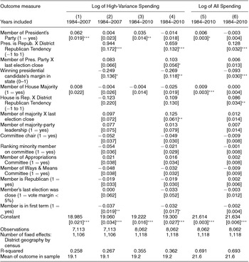
Table 1 presents the results from different specifications of the pooled cross-sectional regression specified in equation (1). (See the Online Appendix for summary statistics of all models.) The dependent variable in columns 1–4 is the log of domestic outlays (in 2010 USD) directed to a House district from the high-variance programs discussed earlier. In columns 5 and 6 it is the log of all outlays.
Predicting District Allocations, Pooled Cross-Sectional Analysis

Notes: Standard errors clustered at district level in brackets. Observations are district-years. Excludes cases dropped by Berry, Burden, and Howell (Reference Berry, Burden and Howell2010), state capitals, and district-year combinations with multiple occupants. See text for details. All models include year and district geography by census fixed effects.
* significant at 10%; ** significant at 5%; *** significant at 1%, two-tailed tests.
For high-variance spending, we present results for two samples. In columns 1 and 2 we include only spending data from fiscal years 1984–2007 (excluding fiscal years 1993 and 2003 due to congressional reapportionment). This is the same period analyzed by Berry, Burden, and Howell (Reference Berry, Burden and Howell2010) and shows that our initial results are similar to prior work. In the remaining columns, we include three additional years of data, ending with fiscal year 2010. These additional data allow us to include one additional change in party control of the presidency. Because the substantive findings are similar across both samples, we discuss the results from this larger sample.
The column 3 specification accounts only for year and district fixed effects and the concordance between a member's partisanship and that of the president and House majority. This is the reduced form of the specification reported in Berry, Burden, and Howell (Reference Berry, Burden and Howell2010: table 1, column 2). Consistent with that research, the estimated effect of having a House member in the president's party is positive (coeff. = .035) and statistically significant (p < 0.05), whereas having a representative in the House majority does not appear to garner more resources for a district (coeff. = −.004; p = .77).
In column 4, we add the covariates discussed earlier, which produces several novel results. Beginning with the House-specific hypotheses, most results are consistent with those of Berry, Burden, and Howell (Reference Berry, Burden and Howell2010). The effect of being in the House majority on high-variance spending remains small, negative, and statistically insignificant. Although the point estimate for the interaction of House Republican × District Republican Tendency is relatively substantial (coeff. = .11), it is estimated imprecisely (p = .40). Finally, members of the House majority whose last elections were close are predicted to receive about 13% more in spending. Given that the average spending is about $221 million in these data, this implies that these vulnerable members of the House majority receive about $29 million more in high-variance spending. The additional control variables provide little evidence that being in a leadership position in the House is associated with receiving additional resources. First-term legislators do worse (about 3% less in spending, p = .06), as do minority-party members whose last election was close, although the latter effect is far from significant.
Turning to the president, the previously significant positive coefficient on In President's Party is eliminated once these covariates are included in the model. The coefficient of –.014 is both substantively and statistically insignificant (p = .43). By contrast, the coefficient on Republican President × District Republican Tendency is positive and statistically significant (p < .01). The .66 coefficient means that, all else equal, areas that are 10 percentage points more Republican on average receive 7% more in discretionary spending under a Republican president than a Democratic one. To illustrate this substantively, the allocations to a core district where the president won 65% of the vote (e.g., Obama's 2012 vote share in Toledo) rather than 35% (e.g., his vote share in Butler County, Ohio just north of Cincinnati) are predicted to be nearly 20% larger, an increase of $44 million.
We also find that allocations are smaller in less contested states in the presidential election (coeff. = −.27, p < .05). This means that districts in a state that the president won or lost by 10% points receive about 2.7% less in funds, or about $6 million, than districts in nearly tied states. Finally, the point estimate for being vulnerable and in the president's party is .10 (p = .07), which is indistinguishable from the estimated effect of being a vulnerable member of the House majority.
The analysis reported in columns 1–4 of Table 1 is for high-variance programs (9% of all spending). This analysis might not yield much evidence of House majority influence if parties focus on shaping the programs that form the bulk of federal spending. For this reason, in column 5 and 6 we replicate our earlier analysis using all spending. In column 5, which includes only the measures of House majority-party status and alignment with the president, we now find evidence that both the House majority and president increase allocations to same-party seats in the House. However, once we account for the other variables in column 6, these effects evaporate. The coefficient on Republican House Majority × District Republican Tendency is .09 (p = .01). If a district's electorate were 30% more favorable to the House majority party than another district, our results predict it would receive 2.6% more in overall federal spending. Because the average level of spending across districts in this sample is $2.5 billion, the more supportive district would receive $63 million more that year than the other district. As expected, the effect of being a vulnerable member of the House majority is much smaller for overall spending (coeff. = .01; p = .38), the bulk of which is difficult to target to districts held by particular legislators, than for more variable spending. None of the remaining House-related variables in the column 6 specification is statistically significant at conventional levels.
As with high-variance spending, the president does not appear to benefit all same-party members in the House (coeff. = –0.003; p = .47). However, the .13 coefficient (p < .01) for Republican President × District Republican Tendency shows a large marginal effect for changes in a district's electoral composition: a district that is 30% more supportive of the president would receive about 3.8% (or $94 million) more in funds each year. Additionally, spending is also lower in less competitive states—a district in a state that is 10% less competitive is predicted to receive about .9% (p < .01), or nearly $23 million, less in spending. Although both of these estimated coefficients are smaller than those found in the high-variance spending sample in column 4, the much larger baseline level of overall spending means that these marginal effects are substantively larger in real dollar terms. Finally, the effect of being a vulnerable member of the president's party is estimated to be modest and not statistically significant (coeff. = .006, p = .61). In sum, the coefficients for the overall spending models reveal strong evidence that both the president and House shape spending in a way that rewards areas with like-minded electorates and that the president appears to reward key presidential election states.Footnote 17
ROBUSTNESS: DIFFERENCE MODELS
The analysis reported in Table 1 exploits, among other factors, variation in who holds particular House seats. One concern with this approach is that which members lose office may be related to unobserved characteristics that shape their ability both to garner federal funds and win reelection. Absent a direct account of why certain seats change hands, any research design relying on observed changes in who holds a given seat is subject to this concern. For example, legislators are more likely to be elected from areas where their party is electorally stronger, and so changes in legislator partisanship over time are more likely in moderate districts than in more partisan ones. This means that we may be estimating the effect of which party controls a seat from the subset of seats that are competitive rather than from nonmarginal seats. Similarly, changes in which party controls a given seat may be correlated with other election outcomes because partisan “tides” are shared across House and presidential elections. For example, when a new Republican president comes into office with new Republican House members (i.e., exhibits coattails), those new Republican members are more likely to be from Republican-leaning districts than from the more Democratic-leaning places where seats are still held by Democrats.Footnote 18 Likewise, changes in which party controls the House are mechanically correlated with which party controls the majority of marginal seats.
In light of these concerns, we also examine changes in spending when control of the legislature or presidency changes, but the individual holding a particular House seat remains constant.Footnote 19 In this way, we can estimate the effect of being in the majority or aligned with the president without concerns that districts that change hands (perhaps held by weak incumbents) are driving the results. For simplicity, we refer to these as difference models. As before, these specifications include year fixed effects, δ. Additionally, we now redefine our district fixed effect to be District × Individual member fixed effect, so that a district gets a new fixed effect, α, when redrawn or when the individual holding the seat changes. These estimates use equations (2) and (3):
-
(2) Yit = β0 + αi + δt + ΨHouse Positionit + β1In House Majorityit + β2Republican House Majorityt × District Republican Tendencyit + ɛit
-
(3) Yit = β0 + αi + δt + ΨHouse Positionit + β1In President's Partyit + β2Republican Presidentt × District Republican Tendencyit + ɛit
In equation (2), which examines the effect of changes in institutional control of the House, our analysis is restricted to members who serve in both the House majority and minority. This analysis therefore relies on members who serve in the House after being elected in both 1992 and 1994 (the switch from Democratic to Republican control) or after being elected in both 2004 and 2006 (the switch from Republican to Democratic control). In equation (3), which examines the effect of change in party control of the presidency, our analysis is restricted to members who serve under both a Democratic and Republican president. This analysis relies on members who are elected in both 1998 and 2000 (a transition from a Democratic president to a Republican one), as well as those who are elected in both 2006 and 2008 (a transition from a Republican president to a Democratic one). Given that districts are redrawn each decade, these specifications discard a great deal of data. (We estimate effects using 529 members for equation [2] and 570 for equation [3].) Additionally, because we fix partisan control of one branch in these specifications, the fixed effects absorb all terms involving partisan control of that branch.
Although the difference models mitigate some concerns associated with a cross-sectional design, certain limitations remain. For example, members in the analysis are becoming more senior over time (changes in leadership are measured using the control variables), but we do not observe the effect of institutional changes for those more marginal members who do not retain office. Additionally, among districts where the same representative remains in office, we assume that there are no unobserved factors (e.g., changes in constituency preferences) that independently shape spending and are correlated with which party controls the presidency or House. These are, in general, weaker assumptions than those made in prior work. However, violations of these assumptions would bias the estimates.
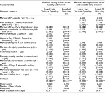
The estimates derived from equations (2) and (3) appear in Table 2. The first two columns examine allocations to districts whose members serve in both the House majority and minority while the presidency remains controlled by one party. In the last two columns, we fix control of the House and examine allocations to districts whose members serve under presidents of different parties. For each analysis, we first examine high-variance spending (columns 1 and 3) and then all spending (columns 2 and 4).
Predicting District Allocations, Difference Design

Notes: See Table 1 for notes. Columns 1 and 2 are restricted to members serving in both House majority and minority. Columns 3 and 4 are restricted to members serving with both same- and opposite-party president. All models include year and district geography x same member x census x change in party control of other institution fixed effects. See text for details.
Focusing first on columns 1 and 2, we now find suggestive evidence that being a member of the House majority is associated with additional overall spending, although measured imprecisely. Per column 2, being in the House majority is associated with about 1% (p = .09) more in federal spending ($28 million). The effect of Republican House Majority × District Republican Tendency is 65% smaller than the corresponding Table 1 estimate and is no longer statistically significant (coeff. = .04; p = .38). We also continue to find evidence that districts in less competitive presidential election states receive less in overall spending, but the magnitude of this effect is now substantially larger. The only other coefficient that is statistically significant in either columns 1 or 2 is the indicator variable in column 1 for being a member of the House leadership. These districts receive 34% more (p < .05) in high-variance outlays than other districts, an effect that seems very large and is not apparent in column 3.Footnote 20
In columns 3 and 4, we focus on members who serve in a House controlled by one party, but experience a change in the party of the president. As in Table 1, we continue to find no evidence that members of the president's party in the legislature receive additional resources—there are borderline significant negative estimates of being in the president's party (p = .06 and .10, respectively). Instead, the positive coefficients for Republican President × District Republican Tendency persist for both high-variance and overall spending, with magnitudes indistinguishable from those in Table 1. That the effect is very similar whether we look at all districts or only those seats that do not change hands is reassuring, because it suggests that both modeling approaches capture the same empirical pattern. Also, as in Table 1, districts in states that were more competitive in the presidential race receive more spending, but the effect is only statistically significant for the overall spending measure. Finally, the coefficient estimates for being a vulnerable member in the president's party are similar to those found in Table 1, but are no longer significant (p = .22 and .13, respectively). There are no other statistically significant results in the column 3 specification. In the column 4 sample, there are two borderline significant results. Being a committee chair is predicted to reduce overall spending by 1.9%, and ranking minority members are predicted to receive 1.2% more in overall spending. Neither effect is robust to the column 2 or Table 1 specifications.
To summarize, the results in Table 2 are similar to those in Table 1 with regard to evidence of the president's influence on resources. Spending is higher in areas where the electorate is more supportive of the president, in more competitive presidential states, and (perhaps) for vulnerable incumbents of his party; but we find no evidence that presidents benefit all same-party members. In terms of the importance of the House majority, we find weaker evidence that the House majority enacts policies that benefit supportive electoral constituencies and its vulnerable members, but novel evidence (with statistically imprecise estimates) that representatives in the House majority party secure more overall spending for their districts.Footnote 21
ADDITIONAL ROBUSTNESS CHECKS
Although our research design allows us to make progress in understanding the degree to which the House majority and president reward districts with co-partisan legislators or supporters in the electorate, it also makes direct observation of patterns in the data difficult. One concern is the source of variation in the key independent variables and, in particular, whether sufficient leverage exists to distinguish legislator partisanship from voter partisanship given the correlation between these variables.Footnote 22
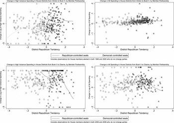
We address this issue in three ways. The first is provided by our difference models presented earlier. Second, we find that the relationship between presidential partisanship and spending holds when analyzing the data graphically. In Figure 1, we plot on the y-axis the change in log spending (log spending at time t minus log spending at time t–1) for individual House members who remain in office when partisan control of the presidency changes, thereby holding most other sources of spending constant. The left panels display the data for high-variance spending, whereas the right panels display it for total spending.Footnote 23 The x-axis is District Republican Tendency. Each point is labeled D or R for which party controls the House seat. The solid line is the lowess (locally smoothed regression line) relationship between District Republican Tendency and the change in spending for Republican-held seats, whereas the dotted line displays that relationship for Democrats. The top two panels plot change in spending for a transition from a Democratic to Republican president (Clinton to Bush II), whereas the bottom two panels display the data for a change from a Republican to a Democrat (Bush II to Obama).
Change in Spending Associated with Change in Party Control of Presidency by District Republican Tendency

For both high-variance and total spending, two results stand out. First, there is a clear relationship between change in control of the presidency and change in average spending. That is, the lowess lines are upward sloping in the top panels, meaning more Republican places experience larger increases in spending when a Republican assumes office, and downward sloping in the bottom panels. Second, there is little evidence that members of the president's party do better than members of the opposition. For example, in the top left panel, the solid line showing the relationship for Republican-held seats is generally below the dotted line for Democratic-held seats in the area of district partisanship for which they overlap.
The third robustness check examines the range of district partisanship for which both Democrats and Republican House members are elected and sees how many members of the legislature fall into this “overlap.”Footnote 24 In light of changes in the range of district partisanship that provide “common support” for both parties, we repeated our regression analyses but eliminated all cases outside of this overlap region. To summarize those results (see Online Appendix Table A10), the only substantive difference is that the coefficient on the interaction House Republican × District Republican Tendency is no longer significant in explaining overall spending. These robustness checks suggest that the correlation between legislator and district partisanship does not explain the lack of evidence that presidents target additional spending to all same-party House members.
DISCUSSION AND CONCLUSION
What consequences do election outcomes have for the distribution of federal resources? In this article we examine the geographic allocation of federal resources in order to understand whether and how the president and members of the House shape federal spending. Our empirical analysis shows that the party of the president has significant implications for where federal resources are directed. Presidents appear to shape policy in such a way as to favor competitive states from the last presidential race and places where they enjoy stronger support in the electorate. For same-party House members, the fact that presidents appear able to direct spending toward places with like-minded voters will tend to reward that party's House members more than the opposition, but there appears to be no additional advantage to shared legislator partisanship except in the targeted case of when a member is electorally vulnerable.
For the House, we show a similar relationship between which party controls the majority and spending in places with different electorates. Places where the majority is stronger in the electorate receive more overall spending than places where it is weaker. Additionally, there is also evidence that members of the House majority receive about 1% more in overall spending than members of the minority, although this result is statistically significant only in our difference design. Finally, vulnerable incumbents in the House majority, as with vulnerable members in the president's party, seem to receive more in high-variance spending than other members.
These results have important implications for our understanding of how Congress and presidents influence federal spending. First, they show that some of the key differences between party control of these institutions and spending manifest in overall federal spending, rather than in the high-variance programs that are the focus of some prior work. Because the bulk of federal spending is not readily subject to ex post influence or discretionary implementation, this implies that political influence also takes place through statutory program rules and control of appropriations, which is consistent with ideological models of policy making in which partisan control of the presidency and House shapes interbranch bargains that alter policy outcomes (e.g., Krehbiel Reference Krehbiel1998).
Second, these results highlight the contingent nature of partisanship as a coordinating device in the American political system. Although both the House majority and the president are associated with policies that generally favor like-minded voters, simply having a same-party president and House member does not appear sufficient to generate additional overall spending. Why not? The best argument is likely one about the difficulty of efficiently targeting districts. Most of the time, presidents who pursue programmatic changes that favor their electorate will also reward their party's House members. When those goals are at odds, however, the bulk of federal spending (the 91% that is low variance) is not readily amenable to geographic targeting to districts represented by particular legislators (including through ex post manipulation) nor subject to annual appropriations review. In light of this, presidents appear far more judicious in taking steps to reward same-party House members, restricting their efforts to targeting more variable spending to vulnerable same-party incumbents. The House majority also appears to shape high-variance spending to reward its vulnerable members, although there is some evidence that overall spending is also increased in all majority-party districts (most clearly in the difference design). Perhaps because legislation is subject to majority-party review, the majority seems apt to supplement policies targeted at voters with those targeted at majority-party districts.
More broadly, our work also highlights some implications for the way in which election outcomes affect the benefits that flow to “swing” and “core” voters. Of course, our analysis concerns aggregate spending in districts—Cox (Reference Cox and Shapiro2009) highlights this distinction—but it reveals that the stakes are far larger for core than swing districts, because the former experience much larger shifts in spending with control of the House and presidency than the latter. Presidents, of course, are largely elected by state, and so policies that reward core areas more than swing ones may be justified as a means to electoral success if, for example, resources are more efficient in mobilizing than persuading (Nichter Reference Nichter2008), subject to the caveat that swing states also appear to be targeted. But for a legislative majority that can maintain its majority only by holding “marginal” seats in less supportive areas, failing to aggressively target marginal areas (rather than just marginal incumbents) may endanger its majority status. One explanation is that majority status is not the only goal of elected officials (see, for example, Snyder Reference Snyder1991), although we note that the effect of voter preferences on spending is weaker for the House than the president and that the House majority also appears to allocate some resources to all of its members.
In closing, we highlight three areas for future research. One is to consider how party representation in and party control of the Senate affect federal spending. However, such an undertaking would likely require different analyses (e.g., Lazarus and Steigerwalt Reference Lazarus and Steigerwalt2009). As we note earlier, our data exclude resources that flow to state capitals for important theoretical reasons. Yet, senators are arguably far less concerned about targeting specific geographic areas in their state than they are in bringing home rewards for their entire state, including those awards that flow through state coffers (Lee and Oppenheimer Reference Lee and Oppenheimer1999). Additionally, malapportionment in the Senate makes forming majorities across chambers subject to concerns about the “costs” of attracting the votes of senators from states that differ widely in their population (Lee Reference Lee2000). Although a full treatment is beyond the scope of this article, we do consider whether Senate-related variables affect the results of our analysis. In Table A11 in the Online Appendix, we repeat our regression analysis with variables indicating the number of senators representing each district who are in the Senate majority party as well as the number in the president's party. Including these variables, however, does not affect the results.
A second area is to examine more fully how geographic targeting occurs and which individual citizens it affects. That is, if Republican presidents are associated with directing resources to Republican-leaning places, are those benefits in general experienced by individual Republicans? Alternatively, is geographic targeting somewhat crude, in that most individuals in those areas do better regardless of their partisanship (and the characteristics associated with partisanship)? Such an analysis is not possible with these data, but as more micro-level data on government spending become available, it may be possible to link individuals to the benefits they receive. Similarly, given that vulnerable incumbents in both the president's party and in the House majority receive additional high-variance spending, it seems likely that ex post influence on policy implementation is an important mechanism. But specifically, how does such influence take place? For example, is it through the implicit threat of changes in appropriations or statutory authority, White House review of bureaucratic decisions, or the appointment process (e.g., Bertelli and Grose Reference Bertelli and Grose2009)? Given issues of observational equivalence in trying to tease out these different pathways, additional data will be needed (along the lines of Gordon Reference Gordon2011) to measure the relative importance of these different mechanisms.
Finally, moving outside of the domestic context, the approach we present here may be fruitful for understanding the relative influence of legislative and executive partisanship in shaping the allocation of resources in different presidential and parliamentary systems. In parliamentary systems with geographically fixed single-member districts, leaders are selected from among the legislative body and therefore have electoral incentives tightly aligned with holding the individual seats necessary for their majority. Thus, it is likely that parliamentary leaders in these systems have stronger incentives than presidents to focus resources on districts their party needs to maintain its majority, whereas presidential candidates can build electoral coalitions independent from those of their legislative allies. By contrast, in proportional representation parliamentary systems, the connection to individual localities is likely less important than ties to groups of voters (Carey and Hix Reference Carey, Hix, Htun and Powell2013). Assessing these sorts of predictions, however, requires similarly rich data from other countries.
Supplementary materials
To view supplementary material for this article, please visit http://dx.doi.org/10.1017/S000305541400063X




Comments
No Comments have been published for this article.