

In the simplest clinical trial we are interested in the difference between a new treatment (T) and a control treatment (C). To try and answer that question, subjects are measured at two different times—before and after treatment (or pre and post)—giving scores of T 1 and T 2 for patients who receive the new treatment, otherwise C 1 and C 2.
One way of expressing the difference between treatments is to ask ‘do the patients differ on their post scores’, that is, does the mean of T 2 differ from the mean of C 2. Another way is ‘do the patients differ on their change scores’, that is, does the mean of T Δ = T 1−T 2 differ from the mean of C Δ = C 1−C 2.
However the question is put, a frequent additional question is whether the pre scores are associated with the post scores or the change scores and if so, whether differences between the two treatments can be attributed to any pre score differences. Such considerations lead to the analysis of covariance, which we will discuss in the next article. Here we will simply look at the association.
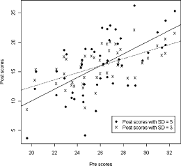
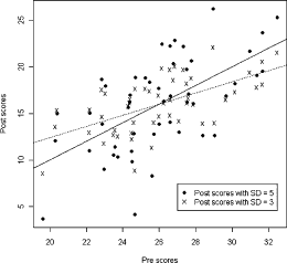
As example, consider a group of patients receiving T whose scores on some measure decrease from a mean of 26 (SD = 3) to a mean of 16 (SD = 5). This is fairly representative as in many clinical trials, patients at entry are fairly similar because of the entry criteria based on severity, whereas at the end of the trial, they are more diverse. The correlation between T 1 and T 2 is 0.6—this is probably higher than usual. We can see these scores plotted in Fig. 1 along with a regression line.
Scatter plot of pre and post (r = 0.60).
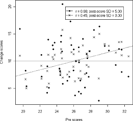
The scatter plot between pre and change (between T 1 and T Δ) is plotted in Fig. 2 along with the regression line. The correlation turns out to be effectively 0—a value (perhaps surprising) that reminds us that pre-post correlations tell us little about pre-change correlations.
Scatter plot of pre with change.
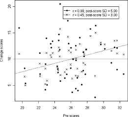
We now change our T 2 scores by reducing their SD such that both SDs are now equal to 3 and these scores are also plotted in Fig. 1 but using a different symbol. The correlation between T 1 and T 2 is unchanged, but although the same in both cases, the regression lines differ because of the different SDs.
The correlation between T 1 and T Δ (see Fig. 2, again with different symbols), however, is now equal to 0.45, a large change induced simply by altering the SD—a result that might again be surprising. The reduced variance of the new T 2 scores, which can be seen in Fig. 1, is paralleled by a reduced variance of the T Δ scores, visible in Fig. 2.
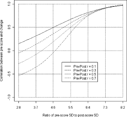
It turns out that the correlation between pre and change depends on the pre-post correlation and the ratio of the pre and post SDs. In Fig. 3 we have plotted how the correlation between T 1 and T Δ changes as the ratio of the two SDs (SD1 and SD2) changes. This has been done for three cases: where the correlation between T 1 and T 2 is 0.3, 0.5 and 0.7. As can be seen, the larger positive correlations occur when the post scores have a smaller SD than the pre scores. When post scores have a larger SD correlations can become negative—potentially substantially so—again an outcome that can be unexpected. Note that these results are not being affected by the means: the mean of the post scores is the same in both cases as is the mean change.
How correlation between pre and change is affected by pre and post SDs.
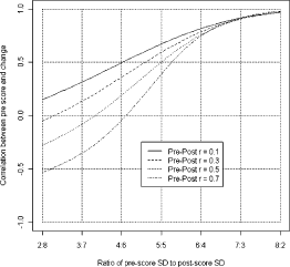
As mentioned, in clinical trials it is not unusual for post scores to be more widely dispersed and so it is not unusual that, if we examine the relationship between pre scores and change, we find that the higher the pre score the smaller the change, the more so indeed, the greater the correlation between pre and post.
This is not a general observation, but peculiar to the correlation of one score with the difference between that score and another. The observed correlations are often not what we would expect and can seem quite counterintuitive.