





1. Introduction
Plasma/laser wakefield acceleration uses high-energy particle/laser beams to generate oscillations in plasma, which in turn creates longitudinal electromagnetic fields that accelerate charged particles (Tajima & Dawson Reference Tajima and Dawson1979; Chen et al. Reference Chen, Dawson, Huff and Katsouleas1985). If the magnitude of the group velocity of the high-energy beam is close to the speed of light, then the phase velocity of the plasma waves would also be close to the speed of light, therefore maintaining acceleration over a relatively long distance (Joshi & Katsouleas Reference Joshi and Katsouleas2003). It has been proved to be a highly feasible and efficient alternative from conventional accelerators, as shown in various experiments (Blumenfield et al. Reference Blumenfield2007; Litos et al. Reference Litos2014; Corde et al. Reference Corde2015; Adli et al. Reference Adli2018).
To predict the effects of plasma acceleration experiments and improve the design of plasma wakefield accelerators, computer simulations are essential. The particle-in-cell (PIC) algorithm (Dawson Reference Dawson1983; Birdsall & Langdon Reference Birdsall and Langdon2018) is a mainstream method for simulating plasma-based acceleration. It discretises electromagnetic fields on grid points and self-consistently tracks the motion of particles between grids, and is known for its robustness and efficiency (Joshi, Corde & Mori Reference Joshi, Corde and Mori2020). In experiments, the particle density in plasmas far exceeds the number of particles that a computer can track (Dawson Reference Dawson1983). Thus, each ‘particle’ in a PIC simulation represents many real particles in the plasma.
Generally, the PIC algorithm involves four steps:
-
(i) Initialise the position and momenta of the particles within the computational domain together with the initial electromagnetic fields.
-
(ii) Calculate the charge and current densities at grid points (or midpoints) according to the particle positions and momenta.
-
(iii) Solve Maxwell’s equations to update electromagnetic fields (usually using spectral (Huang et al. Reference Huang, Decyk, Ren, Zhou, Lu, Mori, Cooley, Antonsen and Katsouleas2006; Decyk Reference Decyk2007), finite-element (Bai et al. Reference Bai, Cao, Chu and Zhang2018) or finite-difference (Fonseca et al. Reference Fonseca2002) methods).
-
(iv) Interpolate electromagnetic fields at particle locations and update particle positions and momenta over a time step.
Steps 2–4 are repeated until the program reaches the desired simulation duration.
Popular PIC codes include OSIRIS (Fonseca et al. Reference Fonseca2002), WarpX (Myers et al. Reference Myers2021), Smilei (Derouillat et al. Reference Derouillat2018), EPOCH (Arber et al. Reference Arber2015), etc. However, these ‘fully explicit’ (traditional) (Joshi et al. Reference Joshi, Corde and Mori2020) PIC codes are considered to have too high a computational load due to the full electromagnetic solver (Huang et al. Reference Huang, Decyk, Ren, Zhou, Lu, Mori, Cooley, Antonsen and Katsouleas2006). Therefore, codes such as WAKE (Mora & Antonsen Reference Mora and Antonsen1997), QuickPIC (An et al. Reference An, Decyk, Mori and Antonsen2013), QPAD (Li et al. Reference Li, An, Decyk, Xu, Hogan and Mori2021), HiPACE++ (Diederichs et al. Reference Diederichs, Benedetti, Huebl, Lehe, Myers, Sinn, Vay, Zhang and Thévenet2022), WAND-PIC (Wang et al. Reference Wang, Khudik, Kim and Shvets2022) and LCODE (Sosedkin & Lotov Reference Sosedkin and Lotov2016) use a method called the quasi-static approximation: since particle beams evolve at a much longer time scale than the plasma wavelength, these codes separate the beam and plasma evolution time scales, and ‘pause’ the beam evolution while calculating multiple steps of plasma response (Huang et al. Reference Huang, Decyk, Ren, Zhou, Lu, Mori, Cooley, Antonsen and Katsouleas2006). This approximation brings a considerable speed up to PIC algorithms. QuickPIC, for example, can be
 $10^2$
to
 $10^4$
times faster than a full PIC code (e.g. OSIRIS) (An et al. Reference An, Decyk, Mori and Antonsen2013), while maintaining accuracy for many problems.
Also, advances in computer hardware can bring further speedup. To adapt to evolving computer architectures, PIC codes have been parallelised on both central processing unit (CPU) (Liewer & Decyk Reference Liewer and Decyk1989) and graphics processing unit (GPU) (Decyk & Singh Reference Decyk and Singh2011) platforms. Parallelised PIC programs typically divide the simulation domain into subregions assigned to different processors. Each processor handles particles and fields within its subregion, and particle and field data are transferred across boundaries when needed. These programs show good scaling when run on multiple processors, and can be further accelerated by moving from CPU to GPU platforms.
Currently, many GPU-based fully explicit PIC codes (PIConGPU (Burau et al. Reference Burau, Widera, Hönig, Juckeland, Debus, Kluge, Schramm, Cowan, Sauerbrey and Bussmann2010); Picador (Bastrakov et al. Reference Bastrakov, Donchenko, Gonoskov, Efimenko, Malyshev, Meyerov and Surmin2012); WarpX (Myers et al. Reference Myers2021), etc.) have been developed, and these codes all support the use of multiple GPUs through message passing interface (MPI) communication. Also, the GPU versions of WarpX and Picador both show considerable speedup compared with their CPU versions. However, to our knowledge, the only quasi-static PIC code with GPU acceleration, before our work, is HiPACE++ (Diederichs et al. Reference Diederichs, Benedetti, Huebl, Lehe, Myers, Sinn, Vay, Zhang and Thévenet2022). It achieves parallelisation via the AMReX framework, in which low-level functions are compiled into either CPU vectorised loops or GPU kernels, depending on the target platform. Also, it only supports one GPU for a two-dimensional (2-D) slice, though multiple GPUs can be used for different longitudinal domains via pipelining. Different from HiPACE++, we used CUDA C to directly write GPU kernel/host functions, for finer control of low-level details; also, we maintained the MPI parallelisation of the CPU program (with each slice assigned to one or more MPI rank(s), and assigned a GPU to each MPI rank, so that multiple GPUs can be used for one 2-D slice (QuickPIC also supports longitudinal parallelisation via pipelining).
QuickPIC is based on the UPIC (UCLA parallel PIC) framework (Decyk Reference Decyk2007). UPIC is an open-source framework developed by V.K. Decyk et al. at University of California, Los Angeles (UCLA) to provide optimised components for large-scale parallel PIC codes. It offers common algorithms (e.g. particle momentum/position updates, charge density calculations, field solvers and MPI-based data transfers) and templates for building customised PIC codes. The framework supports multiple programming paradigms, with Fortran 77 for low-level functions, Fortran 90 for encapsulation and C/Fortran 2003 for high-level logic. UPIC also supports MPI-based distributed memory parallelisation, dividing the simulation domain into subregions with an equal number of particles (or volume) assigned to different ranks; shared-memory parallelisation inside a rank is achieved via OpenMP for CPU and CUDA for GPU platforms.
To adapt QuickPIC for GPU-MPI parallelisation, we referenced the PIC-skeleton code within the UPIC framework (Decyk Reference Decyk2015; Decyk Reference Decyk2023). The PIC-skeleton provides a simplified, modular structure for implementing GPU-accelerated PIC algorithms, focusing on core computational components while omitting complex input/output and analysis features. This framework is designed for educational and debugging purposes, allowing developers to isolate and optimise critical functions such as particle pushing, charge deposition and field solving.
In this article, we first review the basic equations in QuickPIC and the structure of the program. Then, we present the revisions of the 2-D loop in QuickPIC. These revisions realise the complete GPU-MPI hybrid parallelism of the 2-D loop which processes the plasma wakefield, and the storage of all wakefield data on GPUs. After revision methods, we report the correctness and speed of the new program under different conditions. Finally, we summarise the performance of the new code and discuss potential directions for future development.
2. QuickPIC algorithm review
In solving for particle movement and field evolution, QuickPIC adopts a coordinate system
 $(x,y,s=z,\xi =ct-z)$
, where
 $s$
represents the penetration depth of the high-energy particle beam, and
 $\xi$
denotes the distance relative to the beam head;
 $x$
and
 $y$
are 2-D orthogonal coordinates in directions perpendicular to beam propagation
 $z$
;
 $c$
denotes the speed of light and t denotes time. Particle movements in plasma are described by
 $x$
,
 $y$
and
 $\xi$
, while movements of the beam particles are described by
 $x$
,
 $y$
,
 $\xi$
and
 $s$
. Under the quasi-static assumption, we consider beam evolution along
 $s$
to be far slower than the plasma response along
 $\xi$
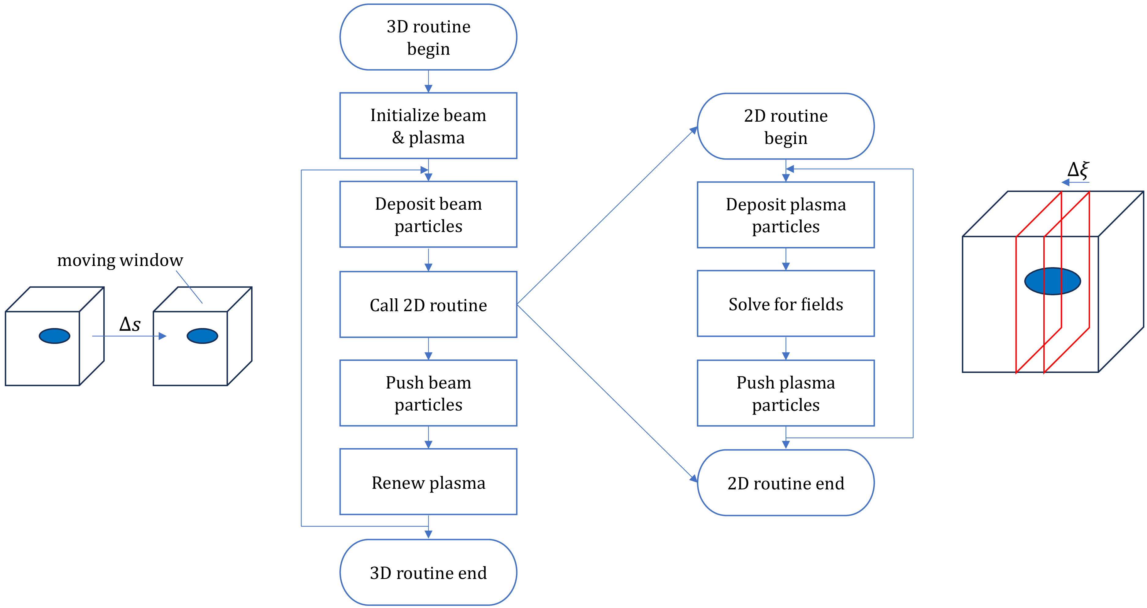
. Therefore, as shown in figure 1, QuickPIC separates beam and plasma computations into 3-D (outer) and 2-D (inner) loops. In each 3-D step, the simulation box is sliced along
 $\xi$
, and a slice of unperturbed plasma is initialised in front of the beam. Then, the slice travels ‘backwards’ in
 $\xi$
, while the evolution in transverse directions is calculated in 2-D steps. In each 2-D step, particles interact via the electromagnetic fields they produce. First, charge and current densities of the particles are deposited onto nearby grid points; then, the fields at grid points are evaluated using a simplified version of Maxwell’s equations, neglecting terms involving
 $\partial / \partial s$
and
 $\partial ^{2}/ \partial s^{2}$
 \begin{equation} \boldsymbol{\nabla} _{\perp } \times \boldsymbol{E}_{\perp } = -\frac {\partial }{\partial \xi } B_z \hat {z} ,\end{equation}
 \begin{equation} \boldsymbol{\nabla} _{\perp } \times ( E_z \hat {z} ) = -\frac {\partial }{\partial \xi } ( \boldsymbol{B}_{\perp } - \hat {z} \times \boldsymbol{E}_{\perp } ) ,\end{equation}
 \begin{equation} \boldsymbol{\nabla} _{\perp } \times \boldsymbol{B}_{\perp } - J_z \hat {z} = \frac {\partial }{\partial \xi } E_z \hat {z} ,\end{equation}
 \begin{equation} \boldsymbol{\nabla} _{\perp } \times ( B_z \hat {z} ) - \boldsymbol{J}_{\perp } = \frac {\partial }{\partial \xi } ( \boldsymbol{E}_{\perp } + \hat {z} \times \boldsymbol{B}_{\perp } ) ,\end{equation}
 \begin{equation} \boldsymbol{\nabla} _{\perp } \boldsymbol{\cdot }\boldsymbol{E}_{\perp } - \rho = \frac {\partial }{\partial \xi } E_z ,\end{equation}
 \begin{equation} \boldsymbol{\nabla} _{\perp } \boldsymbol{\cdot }\boldsymbol{B}_{\perp } = \frac {\partial }{\partial \xi } B_z ,\end{equation}
 \begin{equation} \boldsymbol{\nabla} _{\perp }^2 \left ( \phi - A_z \right ) = - \left ( \rho - J_z \right ) ,\end{equation}
in which
 $\boldsymbol{\nabla} _{\perp }=({\partial }/{\partial x})\hat {x}+({\partial }/{\partial y})\hat {y}$
,
 $\rho$
represents charge density,
 $\phi$
represents electric potential,
 $A$
represents magnetic vector potential,
 $J$
represents electric current density, and
 $\boldsymbol{E}_{\perp }$
and
 $\boldsymbol{B}_{\perp }$
represent the electric field intensity and magnetic induction intensity in the
 $xOy$
plane, respectively. These functions are solved using the spectral method; fields go through fast Fourier transform (FFT) (with sine and cosine as the orthogonal bases) into functions of wavenumbers
 $(k_x,k_y)$
, and are solved as linear equations, then transformed back to functions of
 $(x,y)$
. At last, the solved fields are used to update the positions and momenta of the particles. After each 2-D step, the state of the slice represents the state of the plasma particles in the corresponding
 $\xi$
position after the whole 3-D step. The complete 3-D–2-D loop is shown in figure 1. For parallel computation, each 2-D slice is assigned to one or more MPI ranks. If multiple MPI ranks are used, the slice is separated equally (in area) among them. Parallelisation along the
 $\xi$
direction is also supported via pipelining: the simulation area can be divided along
 $\xi$
into several pipeline stages, each containing an equal number of 2-D slices. One or more MPI ranks can be assigned to a pipeline stage, in which 2-D slices are processed sequentially, and each 2-D slice is dealt with in the aforementioned manner.
Flow chart of 3-D–2-D loops in QuickPIC.

Figure 1. Long description
The flowchart illustrates the 3-D2-D loops in QuickPIC for plasma/laser wakefield acceleration. The process begins with the initialization of the beam and plasma. Beam particles are then deposited, followed by a call to the 2D routine. The 2D routine involves depositing plasma particles, solving for fields, and pushing plasma particles. After the 2D routine ends, the process continues with pushing beam particles and renewing the plasma. This sequence repeats until the 3D routine ends. The moving window concept is depicted with a shift by a distance delta s, and the 2D routine is applied within a slice delta xi.
3. The GPU-MPI parallelisation approach for QuickPIC
3.1. Target analysis
QuickPIC employs a three-layer structure:
-
(i) Bottom layer: Fortran77 functions for basic computations. These functions are based on legacy PIC codes at UCLA, and Fortran77 is chosen for its high performance; it is observed that Fortran77 performs better than any other language (at the time when UPIC and QuickPIC were developed) for it is rather primitive, and compilers can transform and optimise it well. Also, Fortran77 can be called by many other languages. However, it is inflexible and unsafe, and thus these functions need wrappers for more complex operations.
-
(ii) Middle layer: Fortran 2003 classes encapsulating low-level details. These classes include arrays that store particle/field information, and define wrapper functions that call one or more Fortran77 functions, but offer simpler arguments. Also, these wrapper functions can check array sizes (which are hidden at higher layers), check if arrays have been allocated and make use of pointer arrays (which, if used at the Fortran77 layer, would degrade performance).
-
(iii) Top layer: high-level classes combining middle-layer components for convenient calling in the main loop. Both the middle layer and the top layer are object oriented. The procedures in these two layers do not perform any substantial calculations; they merely make decisions and delegate the work to underlying Fortran77 functions (Decyk Reference Decyk2007).
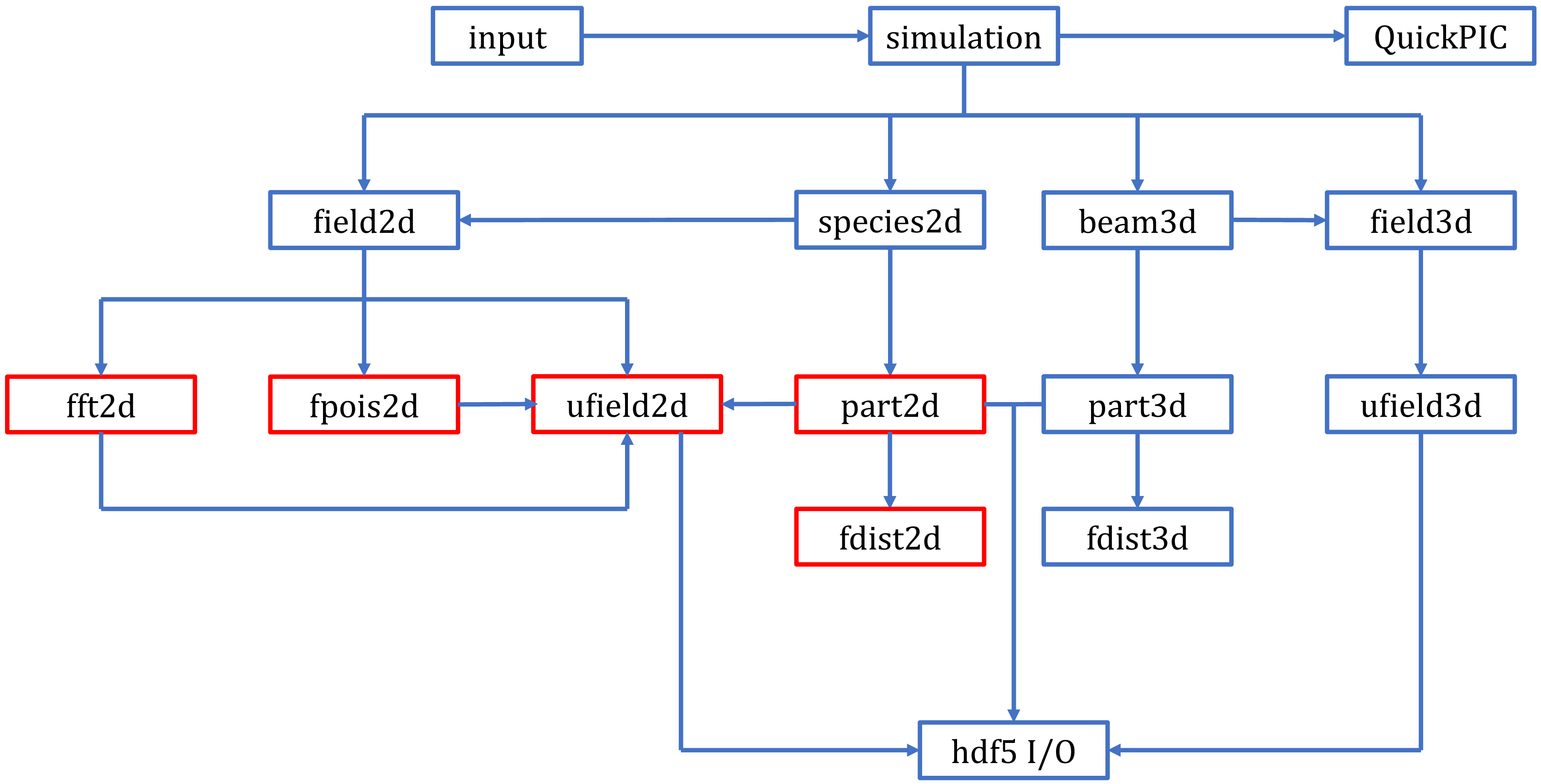
Among all high-level classes, the field2d (electromagnetic fields) and species2d (particles) classes, which are called in the 2-D loop, dominate computational load. The field2d class relies on three mid-layer classes: fft2d (FFTs), fpois2d (Poisson equation solver) and ufield2d (field storage and arithmetic operations). The species2d class depends on the part2d class for particle-related computations, such as charge density calculation, momentum updates and particle migration across MPI boundaries. In addition, the part2d class relies on the fdist2d class for particle array initialisation. The mid-layer classes fft2d, fpois2d and part2d also use the ufield2d class, for they all include read/write operations on 2-D electromagnetic field data. Figure 2 shows the various main classes in QuickPIC, their relationships, and the main GPU revision target classes-fft2d, fpois2d, ufield2d, part2d and fdist2d, in which underlying Fortran 77 functions were replaced with CUDA C functions.
Class diagram of QuickPIC. Classes outlined in red are the main GPU revision targets.

QuickPIC discretises the simulation domain into grids to compute and store field-related information. Grid cells are distributed evenly across non-shared-memory MPI ranks. Particles are inherently discrete, but are grouped by larger subregions called tiles – each containing multiple grid cells. Particles in the same tile are stored next to each other in a particle array, for faster r/w in particle-related operations (Decyk & Singh Reference Decyk and Singh2011).
For a domain with
 $n_x\times n_y$
fine grids, and
 $a$
MPI ranks on one or more physical computing nodes (each rank assigned with
 $b$
CPU cores) assigned to the task,
 $n_x\times n_y/a$
grids are assigned to each rank. The ufield2d class manages electromagnetic field data (e.g.
 $\boldsymbol{E}$
and
 $\boldsymbol{B}$
) at these grid points. Above this, every
 $m_x\times m_y$
grid cells form a tile. The total number of tiles in a rank is
 $m_{x1}\times m_{y1}$
, where
 $m_{x1}=\lfloor (n_x -1)/m_x\rfloor +1$
and
 $m_{y1}=\lfloor (n_y/a -1)/m_y\rfloor +1$
(
 $\lfloor x \rfloor$
denotes the largest integer that is smaller than or equal to
 $x$
). A particle located near the grid cell
 $(n,m)$
belongs to the tile at row
 $\lfloor n/m_x \rfloor$
and column
 $\lfloor m/m_y\rfloor$
. The part2d class managess particle data (e.g. positions and momenta). Both field and particle data are stored in the shared memory of the rank. Each core within a rank processes
 $m_{x1}\times m_{y1}/(a\boldsymbol{\cdot }b)$
tiles; tasks are assigned to these cores via OpenMP. While the number of grid cells per tile is fixed, the particle count per tile varies dynamically during simulation. Thus, the part2d class includes:
-
(i) part: a 2-D array (particle count
 $\times$
attributes per particle) for storing particle positions and momenta.
-
(ii) ppart: a 3-D array (number of tiles
$\times$
maximum particles per tile
$\times$
attributes per particle) for tracking particles within each tile. -
(iii) kpic: an array recording the number of particles in each tile.


These arrays (and other particle-related arrays) are allocated assuming a maximum number (larger than the number of particles initialised) of particles for each MPI rank, to allow for particles moving between MPI ranks, and a rank dealing with more particles than the number at initialisation.
The loops in the underlying Fortran 77 functions (e.g. particle updates, charge density calculations) were replaced with GPU-parallel kernel functions.
3.2. Mapping simulation objects to CUDA architecture
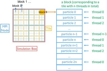
To achieve efficient GPU parallelisation, we established a hierarchical correspondence between QuickPIC’s simulation objects and CUDA’s computational units (threads, blocks, grids). Each MPI rank drives one GPU, which is the common practice of PIC codes with GPU support (Burau et al. Reference Burau, Widera, Hönig, Juckeland, Debus, Kluge, Schramm, Cowan, Sauerbrey and Bussmann2010; Bastrakov et al. Reference Bastrakov, Donchenko, Gonoskov, Efimenko, Malyshev, Meyerov and Surmin2012; Myers et al. Reference Myers2021; Xiong et al. Reference Xiong, Huang, Yuan, Kuang, Sharma, Jiang, Wu and Yu2025). Tiles are assigned to CUDA blocks and particles/grid points are distributed across threads. Take the function gpu_deposit, which calculates charge density at grid points, as an example

In this way, a block with n threads deals with a tile, and the
 $i$
th thread in the block deals with the
 $i$
th,
 $(n+i)$
th,
 $(2n+i)$
th… particles in the tile (Decyk & Singh Reference Decyk and Singh2011), as shown in figure 3. This method has also been applied to other PIC codes (Xiong et al. Reference Xiong, Huang, Yuan, Sharma, Kuang, Jiang and Yu2024). For current deposition (calculation of current density at grid points), the function gpu_amjdeposit has a similar structure, only that the speed of the particle is also read from ppart[].
Mapping of CUDA architecture to particle simulation.

Figure 3. Long description
A diagram of the mapping of CUDA architecture to particle simulation. Panel A: The simulation box is divided into multiple blocks, each containing several tiles. Each block is labeled sequentially starting from block 0. Panel B: A detailed view of a single block corresponding to a tile. The block contains multiple particles, each assigned to a specific thread. The threads are labeled sequentially starting from thread 0. The particles are listed in order, with each particle assigned to a thread in a cyclic manner.
Field interpolation in QuickPIC-GPU is done in the function for pushing particles, gpu_ppush2l. This function first loops over grid points in a tile, to load global fields onto block-level shared memory; then, after a block-level synchronisation, loops over particles in a tile, to calculate field values at particle locations, and update particle positions and momenta

Also, since particles in the same tile are stored next to each other, when they move from one tile to another, they need to be reordered. The pmove() subroutine, which handles this, will be discussed later in the article.
For field computations without tile-level structure, the block number is set to be the maximum number of tasks that can be processed in parallel (for FFT processes, this is usually the grid size in the x or y direction; for other field-related processes, this is usually the total 2-D grid size) divided by the total number of threads in a block (currently set to 64), to best utilise GPU computational power, and minimise the task size of a single thread.
In both particle and field computations, CUDA block- and grid- level synchronisations are needed. For example, block-level synchronisation is needed before block-level shared-memory results in particle deposition being aggregated to global memory; grid-level synchronisation is needed when all blocks need to finish aggregating block-level particle deposition results before moving on to other tasks that would require these results. For block-level synchronisation we use the CUDA call __syncthreads(); grid-level synchronisation is implicitly done when the next task is another kernel call (it would wait in a queue of kernel calls before the GPU is finished with all the calls before it) and a memory copy between the CPU and GPU on the same rank (it would wait until all kernel calls before it are finished on the GPU, and block any kernel calls after it until it is done), and explicitly done by calling cudaDeviceSynchronize() before and after MPI transfers.
3.3. Atomic operations
When porting QuickPIC to GPUs, managing memory access order across threads became critical. Parallelising serial loops into kernel functions risks concurrent thread access to shared-memory addresses, leading to race conditions. For example, in the gpu_qdeposit() kernel, each thread calculates the charge density contribution of a particle to grid points. If multiple particles contribute to the same grid point, threads may simultaneously read, modify and write to the same memory location. Without synchronisation, threads could read unmodified values, resulting in incomplete updates (e.g. only one particle’s contribution recorded instead of the cumulative sum). Problems alike exist in current deposition, field interpolation, etc. To resolve this, CUDA-specific atomic operations (e.g. atomicAdd(), atomicMax()) were employed. These operations serialise access to shared/global memory locations, ensuring that only one thread modifies a target address at a time.
3.4. Host functions
Host functions in CUDA bridge the gap between high-level Fortran 2003 classes and low-level GPU kernels. These functions manage kernel launches, parameter passing and error handling. For example, the fgpu_deposit() host function encapsulates the gpu_deposit kernel

in which dimGrid denotes the number of blocks in a CUDA device (GPU), and dimBlock denotes the number of threads in each block.
Besides, memory management host functions handle GPU memory allocation, deallocation and data transfer.
3.5. Adaptations involving multiple kernel functions and MPI
3.5.1. Rewriting of pmove()
The pmove subroutine handles particle sorting: it sorts the particle array ppart[] once every 2-D step, to ensure that particles in the same tile are stored together, and can be quickly loaded for other particle operations, particle migration across tiles and MPI ranks. The ppart[] array is arranged as follows: the simulation area is separated into mxyp1 tiles, for each tile a maximum of nppmx particles are allowed, and the number of attributes of each particle is dim; therefore, the total size of ppart is dim*nppmx*mxyp1; the attribute l of particle m in tile n can be accessed via ppart[l+m*ndim+n*nppmx*dim], and the actual number of particles in tile n is stored in the nth place in the array kpic[]. Pmove mainly consists of three phases: firstly, the Fortran 77 function ppporder2la loops through all the particles in each tile. Each particle is determined whether it is leaving its current tile, and, if it does, in which direction it is going; the leaving particles and their destinations are stored in the array ppbuff[]; and the vacancies they left (positions in the particle array) is recorded in the ihole[] array. Furthermore, if a particle is determined to be crossing the MPI rank boundary, it is copied from ppbuff[] to another special buffer array. Secondly, particles crossing MPI rank boundaries are transferred via MPI send/receive operations. Thirdly, the ppporder2lb function loops through ihole[], and fills vacancies in each tile with incoming particles read from ppbuff; if incoming particles for a tile are fewer than the holes that departed particles left, the extra holes are filled with particles stored at the end of this tile; if there are more incoming particles than holes in a tile, the extra particles are attached to the end of the storage space allocated for this tile. At the same time, kpic[] is updated (Decyk & Singh Reference Decyk and Singh2011).
In the original code, ppporder2la and ppporder2lb contain multiple OpenMP loops with inter-dependent results. To adapt this for GPUs, each OpenMP loop was converted into a separate CUDA kernel. When these kernels are called by the host, they queue up to be executed sequentially (the next kernel is only executed after all the threads in the GPU have finished executing the last kernel), to ensure that inter-dependent results (e.g. number and positions of leaving particles in a tile) are calculated before they are read by a different thread in a different block. Buffer data are transferred directly between GPUs via CUDA-aware MPI.
3.5.2. Rewriting of FFT transpose
In QuickPIC, for multiple MPI ranks, the 2-D fields are partitioned in the
 $y$
direction, and continuously stored in
 $x$
, by default. For example, for 2 MPI ranks and a 2-D slice with boundaries
 $(-x_b,x_b)$
and
 $(-y_b,y_b)$
, 2-D data in
 $\{(x,y)|-x_b\lt x\lt x_b,-y_b\lt y\lt 0\}$
are stored in one rank, and 2-D data in
 $\{(x,y)|-x_b\lt x\lt x_b,0\lt y\lt y_b\}$
are stored in the other rank. Therefore, 2-D FFT in QuickPIC involves three steps: firstly, 1-D transform is performed in
 $x$
: for the bit-reversal operation, each data point is assigned to a thread; for the iterative combination part, each row in the direction to be transformed is assigned to a block and each combination in an iteration step is assigned to a thread in the block; secondly, the whole field matrix is transposed across the simulation box, so that the field is now continuously stored in
 $y$
; finally, 1-D transform is performed in
 $y$
; the parallelisation method is the same as in the first step (Decyk & Singh Reference Decyk and Singh2011). In order to perform a matrix transpose across multiple ranks, 2-D data needs to be first transposed locally. Some data would be in a different rank when flipped across the main diagonal of the matrix; these are then sent to the corresponding rank(s). Other data would remain in the same rank, and need not be transferred. Similar to pmove, we rewrote the MPI communication functions into the separate C file, and linked them to the CUDA host functions for FFT transpose.
4. Performance evaluation
To evaluate accuracy and speed of the revised program, we tested the program before/after revision using the same input parameters (except for particle density and resolution). All simulations in this section ran on CPU/GPU clusters provided by the Beijing Super Cloud Computing Centre. For CPU clusters, each computing node is equipped with 2 AMD EPYC 7452 processors with 32 cores each; for GPU clusters, at most 8 NVIDIA A100 GPUs (PCIe, 40 GB, 2 computing nodes with 4 GPUs each) can be allocated for a task. The simulation object is a nonlinear plasma wakefield created by a particle beam. The beam is initially placed at the origin, with a distribution of
 $n_be^{-r^{2}/\sigma _{r}^{2}}e^{-z^{2}/\sigma _{z}^{2}}$
; the plasma is initially evenly distributed with a density of
 $n_p$
. The normalised parameters are:
 $n_b/n_p=10.0$
,
 $k_p\sigma _r=0.2$
and
 $k_p\sigma _z=1.0$
;
 $k_p=\omega _p/c$
is the plasma wavenumber, and
 $\omega _p=\sqrt {n_pe^2/m_e\epsilon _0}$
is the plasma frequency. The program ran a single 3-D step, and the number of 2-D steps is equal to the resolution in the
 $z$
direction.
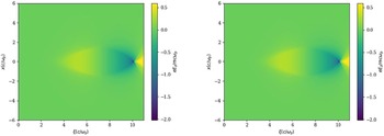
Simulated with the program before(left)/after(right) revision, electric field in direction z (
 $\xi$
), distributed across the x–
 $\xi$
plane.

Comparison of simulation result before/after revision, electric field in direction z (
 $\xi$
), distributed along the z axis. Simulations were conducted with 64 CPU cores (for the old program) and 1, 2 and 4GPUs (for the new program).

Figure 4 shows distribution of
 $E_z$
, simulated by the program before and after revision; figure 5 shows a comparison between on-axis lineouts. We see that there is excellent agreement between these results, and differences are negligible.
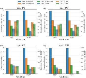
To test the speed performance of the new program, we measured the time taken to run a 2-D loop, with 4/9/25/100 particles per cell, and resolutions of
 $512^3$
(9*9*9 in the input file) and
 $1024^3$
(10*10*10 in the input file). Each combination of ppc and resolution was measured with 8/16/32 CPU cores and 1/2/4 GPUs, though all set-ups except the largest (100 particles per cell and
 $1024^3$
resolution) fit on a single GPU. The results are shown in figure 6. For CPU cases, the more threads we use, the less time the simulation requires; however, for more than half of the GPU cases, one GPU takes less time than 2 or 4 GPUs; also, except for the 100 particles per cell and
 $1024^3$
resolution case, which cannot fit on a single GPU, one GPU takes less time than all CPU set-ups.
Measurement of simulation 2-D time in seconds. Subplots (a), (b), (c) and (d) show set-ups with 4/9/25/100 particles per cell, respectively. Execution time is measured with 8 (blue, plain)/16 (orange, plain)/32 (green, plain) CPU threads and 1 (blue, slashed)/2 (orange, slashed)/4 (green, slashed) GPUs. In each subplot, results with a simulation resolution of
 $512^3$
are shown on the left side, and results with a simulation resolution of
 $1024^3$
are shown on the right side.

Also, since most problems fit on a single GPU, we also calculated and compared the node-hours spent by 32 CPU threads and 1 GPU. For CPU tasks, the number of node hours is calculated as time taken
 $\times$
number of CPU cores/64; for GPU tasks, the number of node hours is calculated as time taken
 $\times$
number of GPUs/4; as each CPU computation node has 64 cores, and each GPU computational node has 4 GPUs. The results are shown in figure 7.
Number of node hours spent in D simulation. Subplots (a), (b), (c) and (d) show set-ups with 4/9/25/100 particles per cell, respectively. Execution time is measured with 32 (green, plain) CPU threads and 1 (red, slashed) GPU. In each subplot, results with a simulation resolution of
 $512^3$
are shown on the left side, and results with a simulation resolution of
 $1024^3$
are shown on the right side.

Figure 7. Long description
Four bar graphs depict the number of node hours spent in D simulation for different setups with varying particles per cell. Panel A shows setups with 4 particles per cell, Panel B with 9 particles per cell, Panel C with 25 particles per cell, and Panel D with 100 particles per cell. Each panel compares execution time using 32 CPU threads (green, plain bars) and 1 GPU (red, slashed bars). The left side of each panel shows results with a simulation resolution of 512 cubed, and the right side shows results with a simulation resolution of 1024 cubed. The y-axes represent node hours, with separate scales for each resolution. The graphs indicate that GPU execution consistently requires fewer node hours compared to CPU execution across all setups and resolutions.
Among all cases that can be run on 1 GPU, the computational time of 32 CPU cores, measured in node hours, is 2.27–3.37 times longer than the computational time of 1 GPU. At the higher resolution (
 $1024^3$
), using 1 GPU instead of multiple CPU cores also lead to a higher speedup, measured in node hours.
It would also be worthy to compare the speed of QuickPIC-GPU with that of a fully explicit PIC code with GPU support, e.g. WarpX. We measured the average number of particle advances per nanosecond, using a single V100 GPU and a resolution of
 $256^3$
(other simulation parameters were the same as the ones given above), to compare with the average number of particle advances per nanosecond when using a single V100 GPU, given in the article (Myers et al. Reference Myers2021). QuickPIC-GPU gives approximately 0.5 particle advances per nanosecond, while WarpX gives approximately 1 particle advance per nanosecond. This difference in update time could have several origins: QuickPIC-GPU uses a 2-D push, not a 3-D one, but the field solve is more complicated due to the quasi-static approximation; QuickPIC-GPU uses a spectral solver, while WarpX uses a finite difference time domain solver. We also note that this does not indicate a comparison of the total simulation time needed for the same physical process, since quasi-static approximation allows for much longer time steps while maintaining accuracy.
5. Discussion
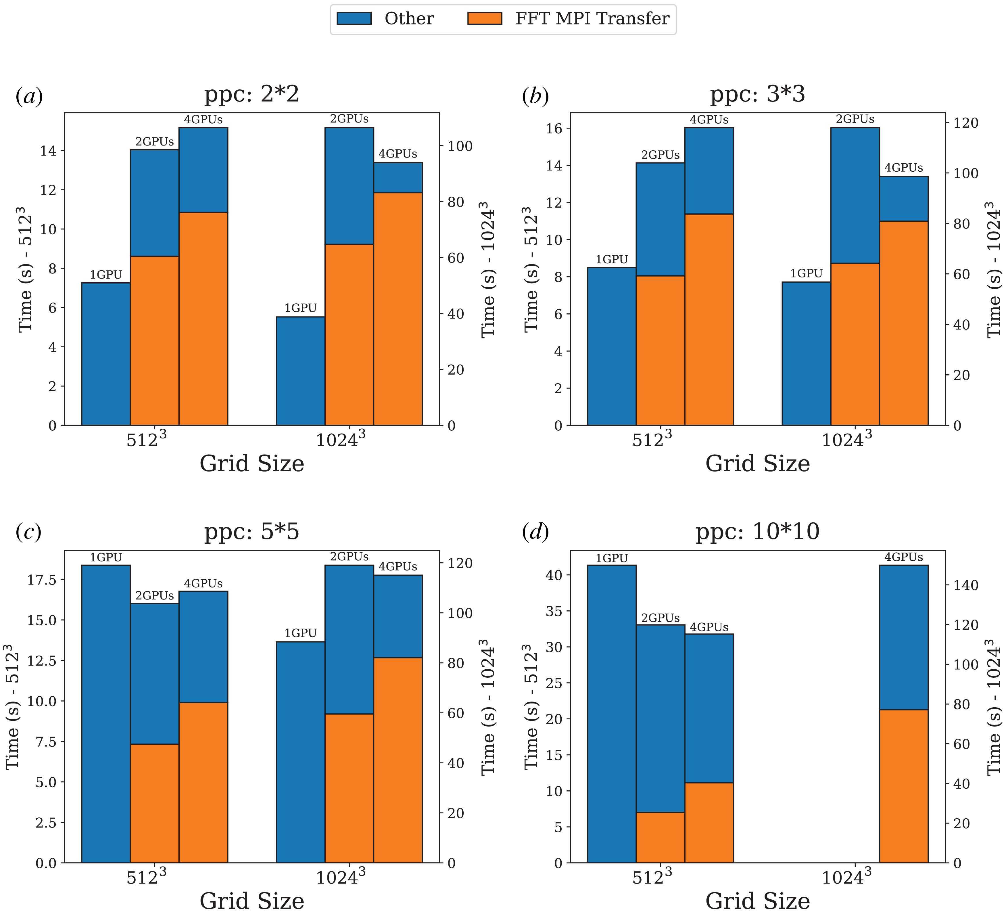
As mentioned in § 3, when using multiple GPUs, the FFT transpose algorithm involves a large amount of data transfer across MPI ranks, in multiple steps. Therefore, we evaluated the computational cost of this transfer by measuring the time spent by these MPI calls, in 2-GPU and 4-GPU runs. The results are shown in figure 8. For comparison, the total time of 1-GPU runs (cross-rank transfers do not exist in these cases) is also shown. We see that MPI transfers take up more than half of the total time, for 2-GPU and 4-GPU runs; after subtracting the time cost of MPI in FFT transpose, the more GPUs we use, the faster other tasks are processed.
Time spent on FFT cross-rank data transfer/other processes. Subplots (a), (b), (c) and (d) show set-ups with 4/9/25/100 particles per cell, respectively. Execution time is measured with 1/2/4GPUs. The FFT MPI transfer time is shown in orange, while time spent on other processes is shown in blue. In each subplot, results with a simulation resolution of
 $512^3$
are shown on the left side, and results with a simulation resolution of
 $1024^3$
are shown on the right side.

Thus, we propose that the field solver in QuickPIC needs to be updated for better performance on multiple GPUs. Suppose
 $a$
MPI ranks are used; in the current algorithm, to transpose across the whole simulation box, each partition is divided into
 $a$
squares in the direction different from the direction in which the simulation box is partitioned. Then, in a loop that runs
 $a$
times, these squares are transposed locally, and then exchanged with squares that are in the symmetric position across the main diagonal of the matrix. Thus, the more MPI ranks used, the more steps FFT transpose would take. For the CPU version, this was not an eminent problem; MPI transfers across CPU threads (which are mostly on the same device) do not take long, compared with other processes (which were not so highly parallel as in the GPU version). However, in the case of multiple GPUs, as seen in figure 8, FFT transpose takes up more than half of the total time.
In the future, there are two optimisation plans that we shall attempt; the first is to use cuFFT, the library for GPU-accelerated FFT algorithms developed by NVIDIA, which currently supports distributing calculation across multiple GPUs, instead of the old FFT algorithm originally designed for CPUs. This would require a change in the parallelisation method of QuickPIC-GPU, and a switch from sine/cosine to
 $e^{ix}$
/
 $e^{-ix}$
as the orthogonal basis. Instead of having each GPU connects to a different CPU, and the CPUs are connected via MPI, cuFFT would require using its own application programming interface to connect multiple GPUs to a single CPU. We shall test if this is applicable to QuickPIC. The second plan is to use finite-difference field solvers that do not include a transpose across the whole simulation box, and thus require less data transfer. Also, we plan to try using the NVIDIA Collective Communication Library (NCCL) for cross-rank transfers, to see if this transfer speed can be further improved.
Besides FFT transpose, other processes also have the potential to be optimised. Currently, the functions in the 3-D loop still run on CPUs, and before and after the call to the 2-D loop in each 3-D step, required data (charge density distribution, electromagnetic fields, etc.) are transferred between the CPU and the GPU; in the future, we plan to also move 3-D particle and field solvers to GPUs, to reduce data transfer and optimise the 3-D loop.
6. Conclusions
We have developed QuickPIC-GPU, a new version of QuickPIC, that runs parallel on one or more GPUs. Referring to the UPIC framework, we use CUDA C functions to replace the Fortran 77 subroutines at the bottom layer, and MPI to communicate between multiple GPUs, each connected to a different CPU. With the same simulation parameters, the results of the new program matches excellently with the old program, using up to 4 GPUs; we see significant speedup (up to 3.37
 $\times$
), when the simulation time (measured in node hours) of 1-GPU runs is compared against that of multiple (up to 32) CPU threads.
When using multiple GPUs, we note that FFT transpose takes up more than half of the total time; in future revisions, we shall attempt to reduce this cost by using cuFFT or finite-difference field solvers. The GPU-MPI parallelisation of 3-D loop functions, and additions of other functions (for example, simulation of laser wakefields; a CPU version is already under development), are also considered for future work.
Acknowledgements
Work supported by Strategic Priority Research Program of the Chinese Academy of Sciences, Grant No. XDB0530000, NSFC Grant 12575156 and 12075030, Beijing Normal University Scientific Research Initiation Fund for Introducing Talents 310432104 and U.S. Department of Energy (DOE), Offices of Advanced Scientific Computing Research and of High Energy Physics (HEP) through the Scientific Discovery through Advanced Computing (SciDAC) project, ComPASS 4, under Contract Nos. DE-AC02-06CH11357 and DE-AC02-05CH11231, and a FNAL subcontract 644405, and by a DOE HEP Grant DESC0010064 and by the U.S. National Science Foundation through award No. 2108970.
Editor Luís O. Silva thanks the referees for their advice in evaluating this article.
Declaration of interests
The authors report no conflict of interest.
 ξ
 ξ

 ξ
 5123
 10243

 5123
 10243
 5123
 10243

 Open access

