1. INTRODUCTION
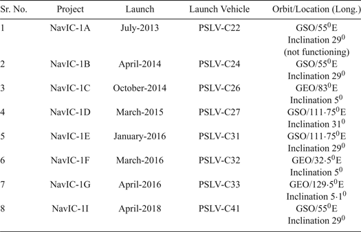
The Navigation with Indian Constellation (NavIC) system was designed by the Indian Space Research Organization (ISRO). The seven satellite NavIC system has three satellites in Geostationary Earth Orbit (GEO) and four satellites in Geo-Synchronous Orbit (GSO) as shown in Table 1. On 12 April 2018, ISRO successfully launched NavIC-1I and completed the constellation of satellites. All these satellites are continuously visible over the Indian region (Santra et al., Reference Santra, Mahato, Mandal, Dan, Verma, Banerjee and Bose2018). The NavIC satellites transmit navigation signals, based on Code Division Multiple Access (CDMA), on the L5 frequency and in the S-band with a Binary Phase-Shift Key (BPSK (1)) modulation for Standard Positioning Service (SPS) users, and with a Binary Offset Carrier (BOC (5,2)) modulation for Restricted Service (RS) users (Zaminpardaz et al., Reference Zaminpardaz, Teunissen and Nadarajah2017; Desai et al., Reference Desai, Jagiwala and Shah2016).
The NavIC constellation

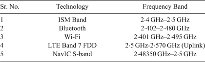
A NavIC receiver operates on dual frequency bands; with the L5 band (1,176·45 MHz) and S-band (2,492·08 MHz) carrier frequencies. Due to spectrum limitations, many communication technologies coincide in similar frequency bands. The frequency of the L5 band is universally assigned to the Aeronautical Radio Navigation Service (ARNS) which is also shared by other navigation systems such as NavIC L5, Global Positioning System (GPS) L5 and Galileo E5 (Dovis, Reference Dovis2015). In addition, the S-band is shared by other communication systems such as Long Term Evolution (LTE), Bluetooth, Wireless Fidelity (Wi-Fi/IEEE 802·11 standard) and the Industrial Scientific Medical (ISM) band as shown in Table 2 (Baghel et al., Reference Baghel, Ingale and Goyal2011). The strengths and weaknesses of navigation in the S-band are briefly described in Mateu et al. (Reference Mateu, Boulanger, Issler, Ries, Avila-Rodriguez, Wallner, Kraus, Eissfeller, Mulassano, Caporale and Germaine2009) and Soualle et al. (Reference Soualle, Bey, Floch, Hurd, Notter, Mathew, Mattos and Mongredien2011). It is important to note that, as a direct consequence of increased carrier frequency, S-band signals are less affected by ionospheric errors than L band counterparts. Similarly, they exhibit reduced phase noise and multipath errors.
Use of spectrum in the S-band

From Table 2, it can be seen that the NavIC S-band signals become more likely to be affected with such multiple technology usage because the signal received from satellites is very weak in nature as the distance between the satellites and Earth is approximately 36,000 kilometres. So, weak signals at the user's receiver are extremely prone to Radio Frequency Interference (RFI) (Dovis, Reference Dovis2015). Among all the technologies described in Table 2, the interference from Wi-Fi signals to the S-band of the NavIC signal is considered: the frequency range of Wi-Fi channel 13 is 2,461–2,483 MHz and the NavIC S-band signal has a frequency range of 2,483·50-2,500 MHz which is nearer to the upper frequency of Wi-Fi (that is, 2,483 MHz) and to the lower frequency of the NavIC S-band signal (that is, 2,483·50 MHz). Although there is a gap of 500 KHz between these frequencies, spurious emissions from Wi-Fi routers creates out of band RFI affecting the received NavIC signal which is studied here.
The detection and mitigation of RFI can be achieved through pre-correlation or post-correlation techniques as described in Dovis (Reference Dovis2015) and Landry and Renard (Reference Landry and Renaud1997):
• In pre-correlation techniques, the antenna, Intermediate Frequency (IF) signal processing, the Automatic Gain Control (AGC) and the Analogue to Digital Converter (ADC) are considered.
• In post-correlation techniques, the Carrier-to-Noise ratio (C/N0), Position, Velocity and Time (PVT) of the input signal affected by RFI are monitored to identify the RFI.
In Marti and Van Graas (Reference Marti and Van Graas2004), the authors implemented a pre-correlation detection method which was applied in two stages: for narrow band interference, the assessment window was obtained from interference-free samples to calculate a threshold at the first stage. At the second stage, a two-sample t-test was computed on the sample mean of a time series to determine the existence of RFI. A similar method has been evaluated in the frequency domain for narrowband RFI (Balaei and Dempster, Reference Balaei and Dempster2009). Both the time and frequency domain detection methods were examined by Tani and Fantacci (Reference Tani and Fantacci2008). In this paper, a detection theory based on hypothesis testing is used to reveal the presence of Wi-Fi interference on the NavIC S-band signal. An assessment window is taken without RFI data and an evaluation window is considered with RFI data. Using these windows, the hypothesis parameters are obtained with two-sample Kolmogorov-Smirnov test (KS- test) (Lehmann and Romano, Reference Lehmann and Romano2006), t-test (Balaei and Dempster, Reference Balaei and Dempster2009) and Variance test (var-test) (Sawilowsky et al., 2002).
Section 2 highlights the analytical modelling of hypothesis testing with various detection methods. In Section 3, a complete description of the experimental setup is presented. The simulation results of Power Spectral Density (PSD), signal at acquisition stage and the detection performance of RFI with the help of different hypothesis testing methods are analysed and compared in Section 4. In addition, this section shows a performance comparison of the KS-test, t-test and var-test methods for detection probability. Finally, the work is summarised.
2. MATHEMATICAL MODELLING
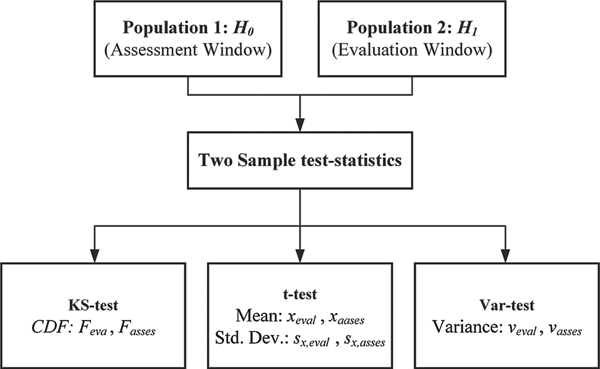
Hypothesis testing is a standard detection method to identify the presence of external interference about a population based on statistical evidence of the sample. Here, the detection of interference is recognised by a two-sample hypothesis test based on distribution, location and dispersion parameters. Population 1 (referred to as an assessment window) and Population 2 (considered as an evaluation window) are obtained from the NavIC signal by considering the interference-free and interference-present environments, respectively. As shown in Figure 1, three detection methods of two sample test statistics are applied to these windows, as described below:
• KS-test: The Cumulative Distribution Functions (CDFs) of assessment and evaluation windows are considered as distribution parameters to analyse this method.
• t-test: The location-based parameters mean and Standard Deviation (SD) are evaluated to make decisions statistically valid in the presence of inference.
• var-test: The variances of the above-mentioned windows are matched to check the presence of interference.
Hypothesis test from two populations.

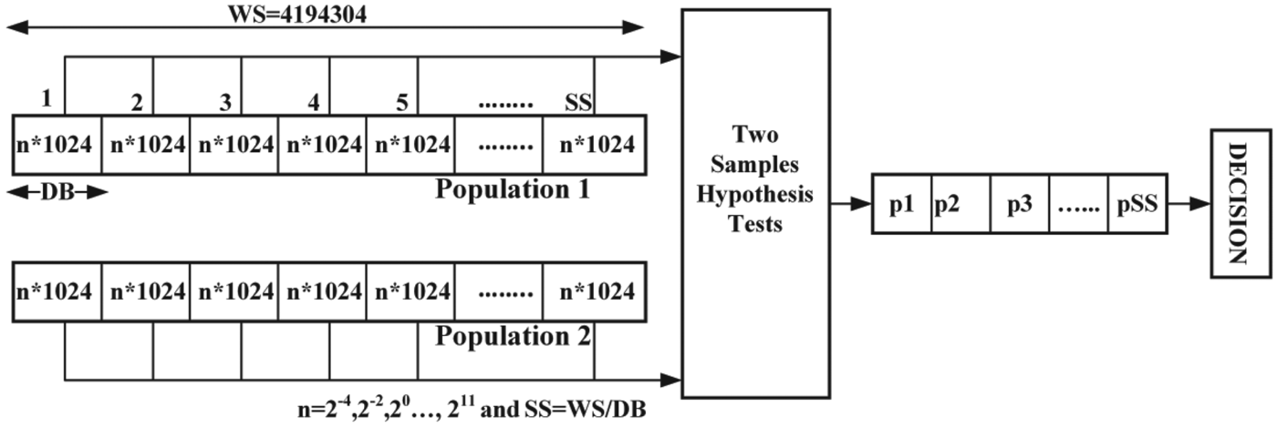
Assume that the total size of the assessment and evaluation window is equal to the Window Size (WS), as shown in Figure 2. Then WS is divided into a number of Data Blocks (DB) which has the number of Sample Size (SS) = WS/DB. For an example, suppose WS = 4,194,304, DB = 2*1,024, then SS = 2,048. The size of WS, SS and DB depends on the sampling rate of the receiver's front-end. Further, the performance of various detection methods is evaluated by the plots of the probability of detection PD versus the processing size of DB and significance level α -alpha.
Process of hypothesis testing.

Regardless of the shape of the population distribution, if the sample size is extremely large, the sample distribution tends to be a normal distribution. So, the Central Limit Theorem (CLT) allows these methods to be used for large samples, even if the two interested populations are not normal (Marti and Van Graas, Reference Marti and Van Graas2004). By observing the behaviour of outcomes such as the p-value (as per Section 2.3 of this paper) and the decision of hypothesis testing between the two populations, further steps are performed to check the interference (Balaei and Dempster, Reference Balaei and Dempster2009).
2.1. Null and alternative hypothesis
The null hypothesis H0 represents the samples acquired without an interfering signal, and the alternative hypothesis H1 represents the samples taken when an interfering signal is present. Here H0 and H1 are complementary hypotheses. In this work, the design of hypothesis is based on the statistical finding of the assessment and the evaluation window. The hypothesis test is presented to confirm the discrepancy between these two population samples. Thus, the null hypothesis is defined as:
 $$H_0 =w_{eval} -w_{asses} =w_d =0 $$
while the alternative hypothesis is defined as:
 $$H_1 ={\rm w}_{eval} -w_{asses} ={\rm w}_d \ne\ 0 $$
where weval and wasses are the sample parameters (according to the hypothesis-based detection method) of the evaluation and assessment windows, respectively, and wd is the difference between these two sample parameters.
2.2. The test-statistic calculation
This section gives different method-based test statistical formulae and points out appropriate decisions for hypothesis testing parameters like CDF, mean, standard deviation and variance. The decision of the hypothesis test depends on the test statistic and the significance level α. Typically, the test statistic is specified by the test type (method) and the significance level α is specified by the sensitivity of the test (usually 0·05). Here, the test statistics are obtained by two-sample hypothesis tests such as a KS-test based on the distribution parameter, a t-test based on the location parameter and a var-test based on the dispersion parameter as described above.
2.2.1. KS-test
The KS-test is a nonparametric hypothesis test that calculates the variation between the CDFs of the two-sample populations over the range of window length in each population. The main features of the KS-test are: first, it is based on the empirical CDF and second it is an accurate test. Furthermore, the distribution of the KS-test statistic itself is independent of the underlying CDF being tested. In this test, the maximum absolute dissimilarity between the CDFs of the two-population window is utilised. So, the test-statistic obtained by a two-sample KS-test is as follows (Lehmann and Romano, Reference Lehmann and Romano2006):
 $$T_{KS} =\mathop {\max }\limits_N \lpar {\vert {F_{eval} \lpar N\rpar -F_{asses} \lpar N\rpar}\vert} \rpar $$
where F is the theoretical CDF being tested. F eval is the proportion to evaluation sample window and F asses is the proportion to assessment sample window. Here N is the total number of samples in each processing window (DB). For this method, the null hypothesis rejection depends on matching the p-value with the significance level α.
2.2.2. t-test
The two-sample t-test is a parametric test and it utilises the location parameter of two independent (evaluation and assessment) population windows. It is used to determine whether two populations have the same mean, where the standard deviations are unknown. The test-statistic is realised using a two-sample t-test as (Balaei and Dempster, Reference Balaei and Dempster2009):
 $$T_t =\displaystyle{{x_{asses} -x_{eval}}\over{\sqrt {\lpar {S_{x\comma asses}^2+S_{x\comma eval}^2} \rpar }}} $$
where x eval and x asses are the sample mean and S x, eval and S x, asses are the sample standard deviation of evaluation and assessment window, respectively. The null hypothesis comes from the two-population window with equal means. The alternative hypothesis decision is based on the p-value which depends on the extreme value of the test statistic and significance level α.
2.2.3. Var-test
This two-sample hypothesis test uses two independent population windows with the assumption of the same variance. It is extremely sensitive to non-normality, which is the major drawback of this method. Let X eval and X asses be identically distributed samples from two independent (evaluation and assessment) population windows. The expected test statistic values for these two populations are non-identical (Sawilowsky et al., 2002).
 $$\bar {M}_1 = \displaystyle{{1}\over{N}}\sum\limits_{i=1}^N {X_{eval}} $$
 $$\bar {M}_2 = \displaystyle{{1}\over{N}}\sum\limits_{i=1}^N {X_{asses} } $$
are sample means and from these:
 $$V_{eval}^2 = \displaystyle{{1}\over{N-1}}\sum\limits_{i=1}^N {\lpar X_{eval} } -\bar {M}_1 \rpar ^2 $$
 $$V_{asses}^2 = \displaystyle{{1}\over{N-1}}\sum\limits_{i=1}^N {\lpar X_{asses}} -\bar {M}_2 \rpar ^2 $$
are sample variances. Then the test-statistic is developed by means of the two-sample var-test is:
 $$T_{var} =\displaystyle{{V_{eval}^2 }\over{V_{asses}^2}} $$
where V eval and V asses are the sample variance of evaluation and assessment windows, respectively. Here, the ratio of the two sample variances is a test statistic. If the population is from a normal distribution with different variances, then the decision is an alternative hypothesis that the ratio deviates from the value 1.
2.3. The p-value calculation
The computable measure of the reporting hypothesis test results is the p-value. In addition, the researchers used statistical measurements of p-values to determine if their hypotheses were correct or not. Also, the experimental results are within the normal range of values, and the observed events can be represented by p-values. Here, the p-value is the probability that the test statistic is at least as good as the extreme value observed when the null hypothesis is observed to be true. A small p-value indicates that the null hypothesis is false. The significance level, denoted by α (=0·05), is the probability of an error in rejecting a null hypothesis which is, in reality, true. Simply, if the p-value is less than or equal to α, then H0 is rejected. If the p-value is greater than α, H0 is accepted. Hence the decision of all detection methods is generated according to the value of H0.
2.4. Performance evaluation of detection methods
It is important to observe which method truly picks out the presence of interference as different types of parameters are tested for this study. A probability plot is a graphical technique used to evaluate whether each detection method gives a true decision or not. In this paper, the detection probability for various detection methods are compared with respect to processing window length and different significance level α. The total data set (WS) remains unchanged, but the probability of detection is measured based on:
• Change in processing window length (DB) by the factor-n as shown in Figure 2, where n = 2−4 to 211.
• Change in significance level α between 0 to 1.
This curve describes the discriminatory power of the various interference detection methods. Thereby, the best detection method can be identified from such types of performance analysis.
3. EXPERIMENTAL SETUP
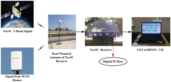
The method used to detect the effect of Wi-Fi interference as a threat to the S-band of a NavIC receiver is described in this section. Digitised IF samples of a NavIC S-band signal were logged using an Accord NavIC receiver which was placed in the Communication Research Lab of the Electronics and Communication Engineering Department, SVNIT, Surat (21·16° N, 72·78° E)(ISRO ICD, 2017; Desai et al., Reference Desai, Jagiwala and Shah2016).
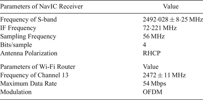
A Graphical User Interface (GUI) was supplied by ISRO and offered a Windows-based real time user interface. A signal strength chart was provided in the GUI and shows the strength of the received signal in terms of C/N0. A TP-Link router (model number TL-WA5210G 2·4 GHz) was used to generate the interference to the NavIC receiver. The experimental setup is shown in Figure 3 and the parameters used for this set up are given in Table 3.
Practical setup.

Specification of NavIC receiver and Wi-Fi router

4. SIMULATION RESULTS AND DISCUSSION
Real time digital IF data (without and with interference) was taken from the front end of the NavIC receiver. This experiment was performed several times to understand the behaviour of RFI. To identify the presence of interference, software simulation was done in MATLAB 2014a. For further analysis, the S-band signals were evaluated as Case I and Case II without and with interference, respectively.
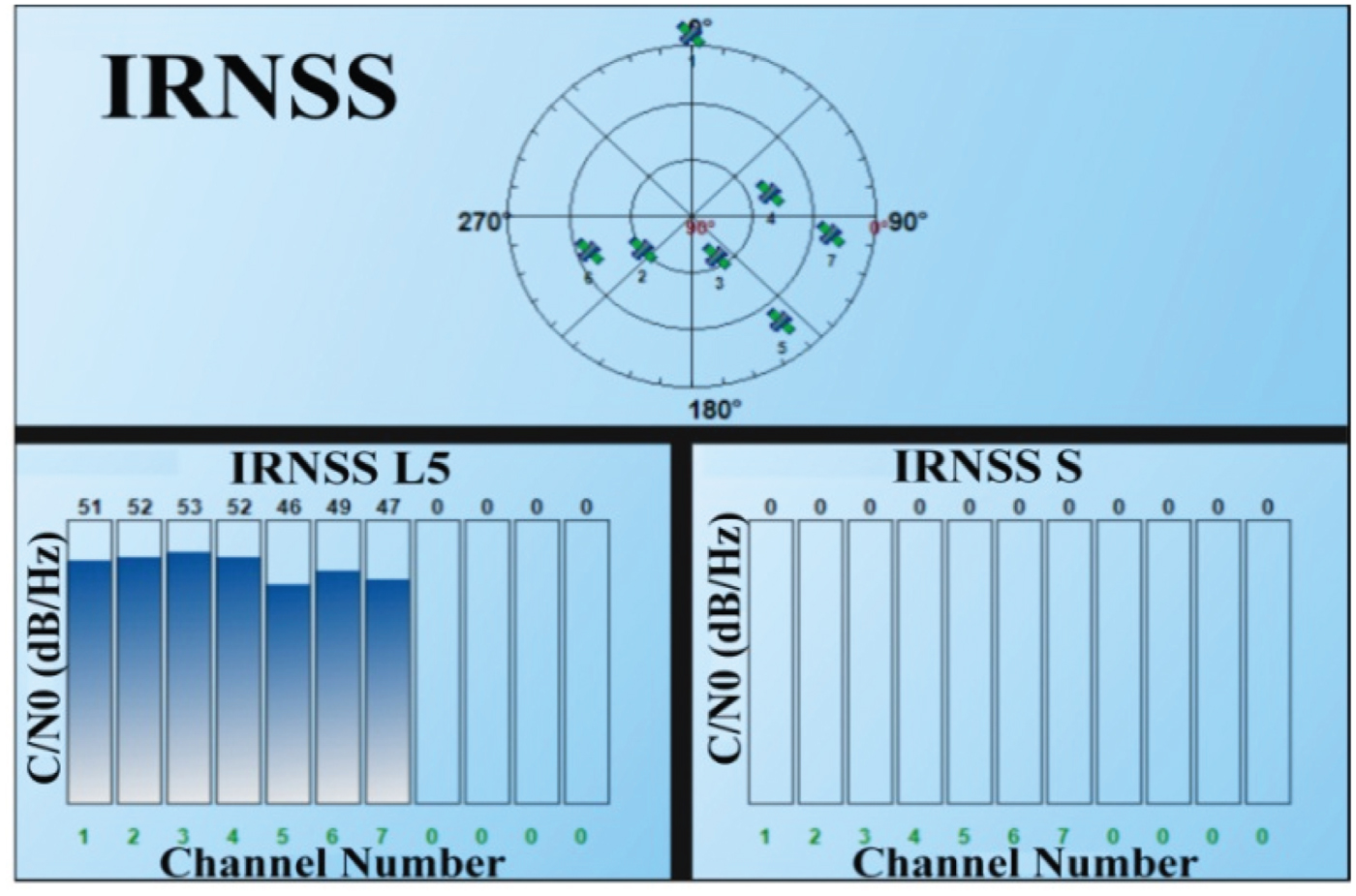
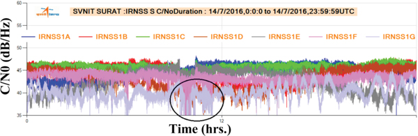
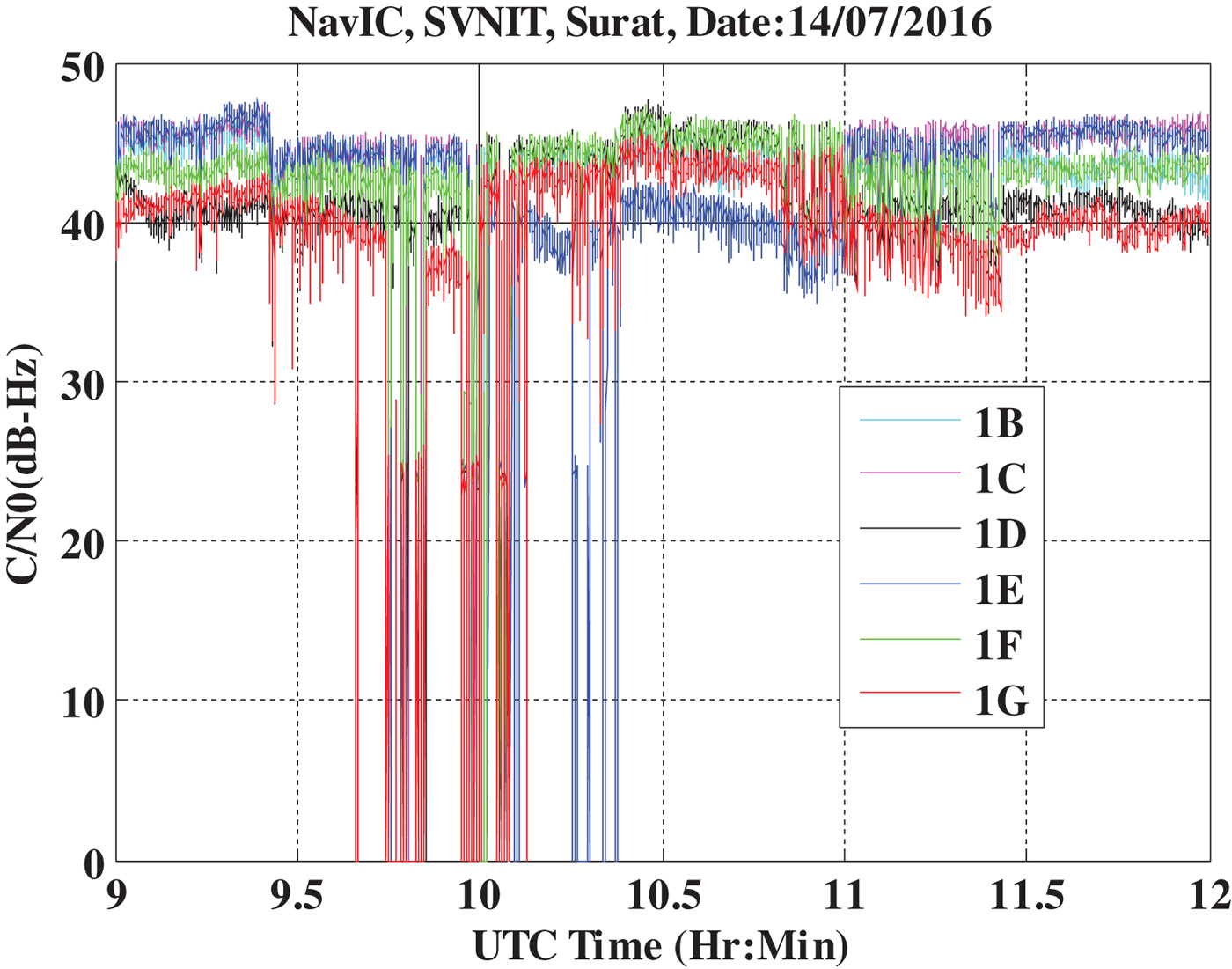
The effect of this interference is identified by monitoring the degraded values of C/N0 as shown in Figures 4–6. It can be seen that the signal strength becomes zero for the particular time duration when the severe effect of interference occurred as shown in Figure 4 (from the GUI). In Figure 5, a graph of all satellites is generated using NavIC Data Analysis Software (IRDAS) version 3·0 (provided by ISRO) for the specific day and time duration when this experimental data was logged. The value of C/N0 decreased only for a certain duration, which is highlighted by the black circle in Figure 5. Figure 6 shows the MATLAB simulated performance of C/N0 values by considering the specific time of interference and it is perceived that the values of C/N0 are reduced and sometimes become zero for the same duration.
Zero Values of C/N0 of S-band signal due to Severe Wi-Fi Interference.

Performance of C/N0 for S-band signal using NavIC Data Analysis Software (IRDAS) version 3·0.

Simulated result of C/N0 for S-band NavIC signal at the time of the experiment.

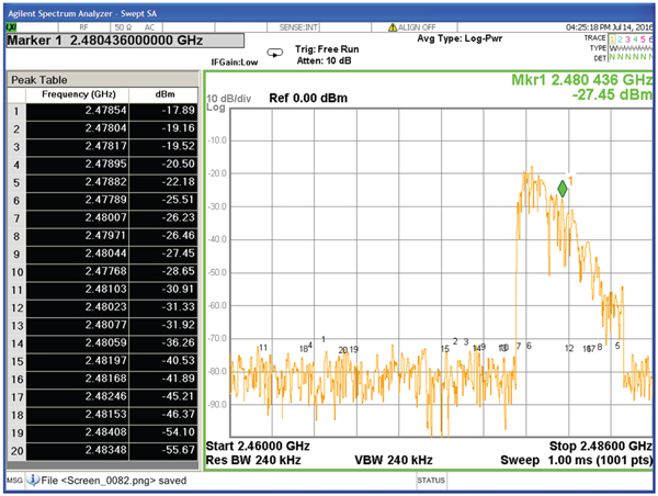
An Agilent N9000A spectrum analyser was used to observe the spectrum of the Wi-Fi router. The spectrum of the router is shown in Figure 7 with a peak table which gives the information of frequency and power. From Figure 7, it is worth noting that the upper band of the Wi-Fi channel 13 is 2,483 MHz, but its spurious emissions exceed this frequency, causing interference to the S-band of the NavIC receiver.
Spectrum of Wi-Fi Signal on Spectrum Analyser.

The other simulated results generated from digital IF data are analysed below.
4.1. Analysis of PSD
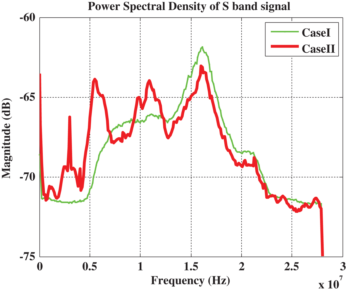
The PSD of the IF data is examined as an initial phase of detection of interference. Figure 8 shows the comparison of the PSD for Case I and Case II. The input signal is divided into M windows that do not overlap, and the length of each window is P as per the Bartlett algorithm. The periodogram is calculated for each window and by averaging the periodograms for the consecutive windows; the Welch power spectrum estimation is obtained. For the N-point sequence X[n], the method is represented as (Fadaei, Reference Fadaei2016):
Performance comparison of PSD for Case I and Case II.

 $$\gamma \lpar k\rpar =\displaystyle{{1}\over{N}}\sum_{i=0}^{M-1} {\left\vert {\sum\limits_{n=0}^{P-1} X_i \lpar n\rpar \exp \left[-j\displaystyle{{2\Pi nk}\over{P}}\right]} \right\vert }^2 $$
where k is the FFT index and:
 $$X_i \lsqb n \rsqb =X\lpar i\times P+n\rpar \comma \; \quad i=0\comma \; 1\comma \; 2\comma \; \ldots M-1 $$
Note that in Case II, the power level of the spectrum is reduced at the centre frequency and other frequency peaks are due to the spurious emission of Wi-Fi interference as shown in Figure 8. Further, it can be observed that lower frequencies of the S-band signal are more affected compared to higher frequencies.
4.2. Analysis of correlation power at acquisition stage
The major digital signal processing stage of the NavIC receiver is an acquisition module that must determine the presence of the signal and provide an approximate estimate of the input signal (Desai et al., Reference Desai, Jagiwala and Shah2016).
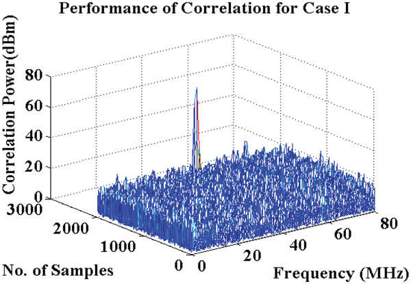
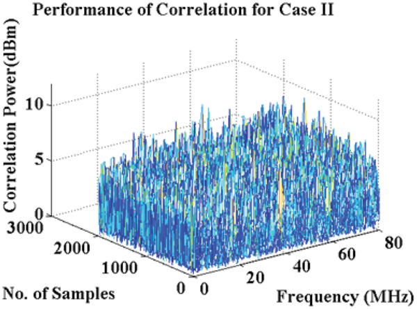
The main task done by the acquisition block is to correlate the input signal with local replicas of the signal code and carrier. If the NavIC signal is present in the absence of interference, a single dominant peak should appear in the cross-correlation process. Figures 9 and 10 compare the cross-correlation power for Case I and Case II. In Figure 10, many peaks have appeared due to interference from the Wi-Fi signal.
Correlation power for Case I at the acquisition stage.

Correlation power for Case II at acquisition stage.

4.3. Analysis of hypothesis testing
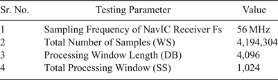
The null hypothesis H0 and alternative hypothesis H1 are taken as defined in Equations (1) and (2) respectively to estimate the difference between two parameters using hypothesis testing methods. The complete process applied to take the decision of hypothesis testing is considered as shown in Figures 1 and 2. For this analysis, the simulation design parameters are considered as per Table 4.
Simulation design parameters

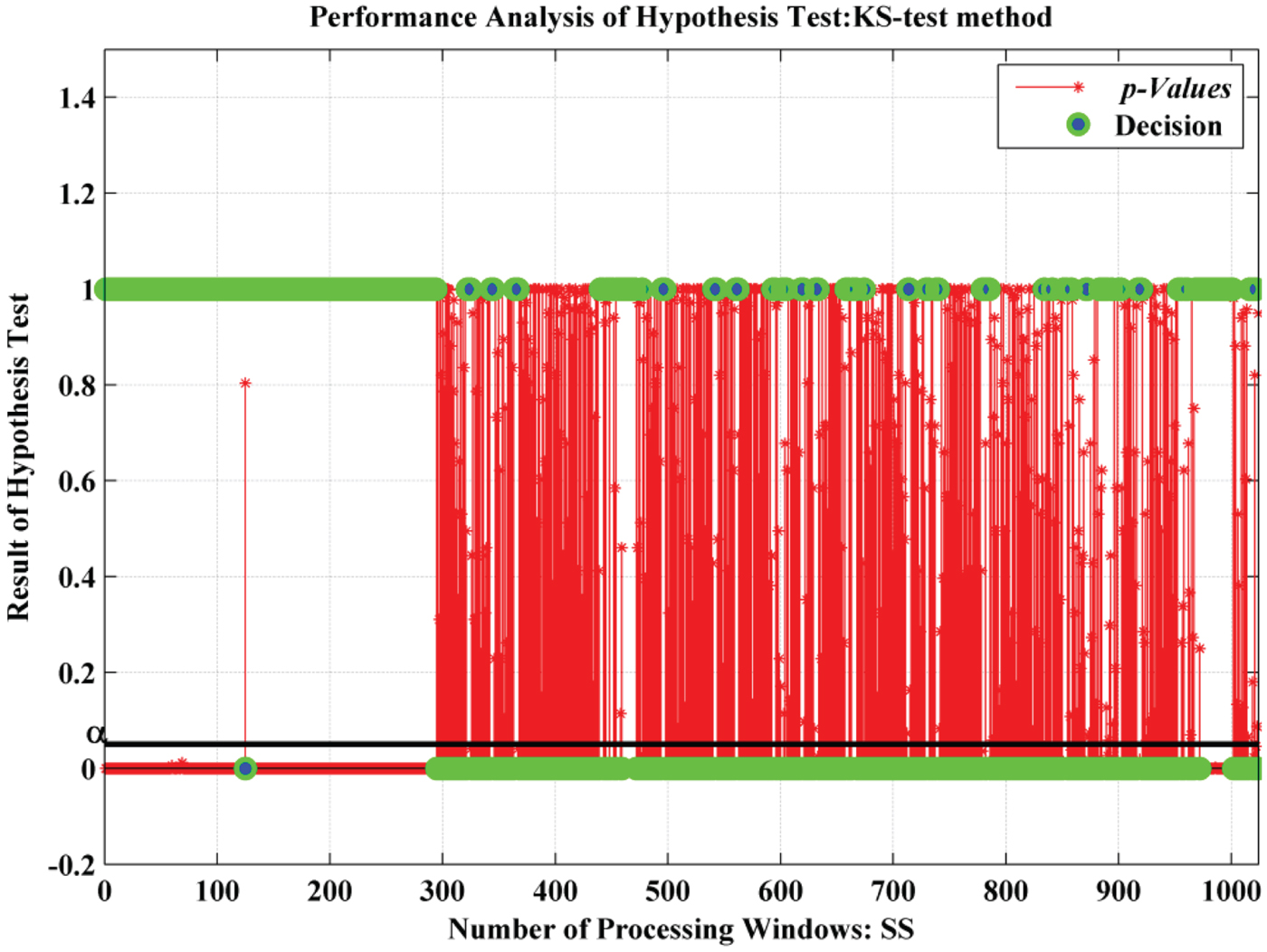
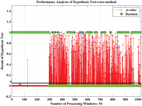
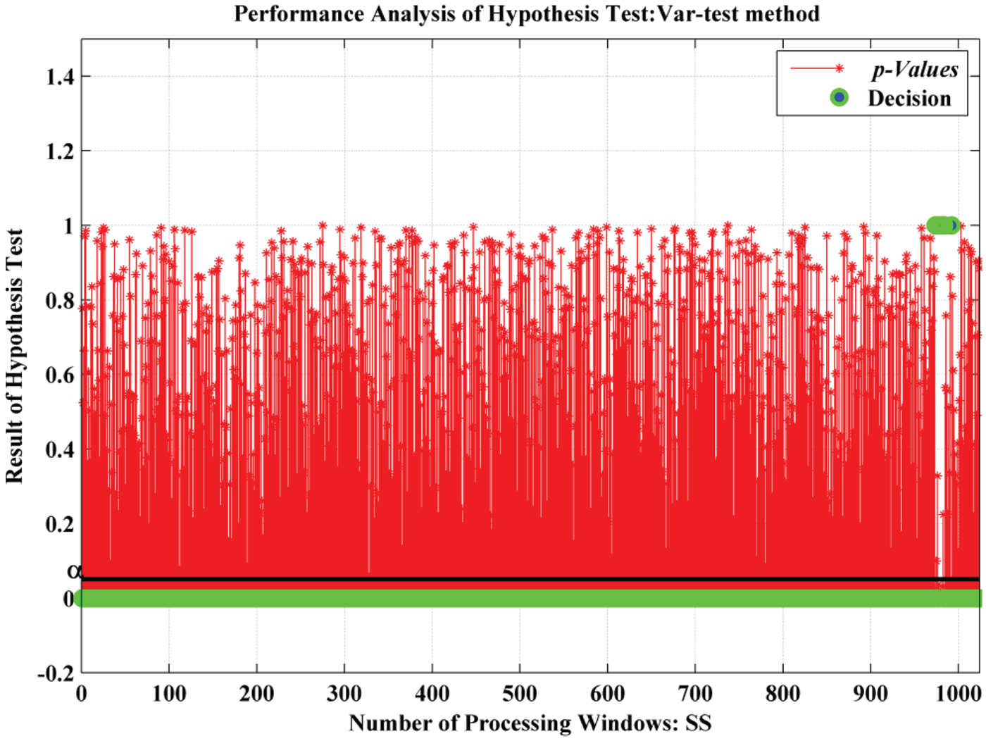
A total of 1,024 processing windows were analysed, and the performance of the KS-test, t-test and var-test detection methods for two sample hypothesis tests were studied. In all detection methods, the p-value was calculated for each window and the behaviour characteristic of the p-value (plotted with red) was observed with a significance level of α = 0·05 (as shown by the black line) (Peck et al., Reference Peck, Olsen and Devore2015). In addition, the decision (marked with green) was generated by consideration of parameters based on detection methods. From Figures 11–13, it is perceived that:
• As shown in Figures 11 and 12, the KS-test and t-test provided a similar level of performance although the p-value is generated by different factors (KS-test depends on α whereas the t-test depends on α and the extremity of test statistics).
• The var-test provided very poor performance with respect to other methods for this study which is revealed in Figure 13. As per Sawilowsky (Reference Sawilowsky2002), this test is very sensitive to the assumption of normality. Due to the unbalanced samples distribution for the processing window length (DB = 4, 096), the generated decision of this test failed to reject the null hypothesis. This can be concluded as the existence of interference not being detected properly by this method.
• The presence of interference was detected in the initial stages of the total processing window of the KS-test and the t-test method observed in Figures 11 and 12.
Performance analysis of p-value and decision for KS-test.

Performance analysis of p-value and decision for t-test.

Performance analysis of p-value and decision for Var-test

4.4. Performance comparison of detection methods
In order to find the best detection method from the two sample hypothesis tests, the measurement curve of PD is analysed. This performance comparison of PD is achieved by changing the processing window length of each method and varying significance level α.
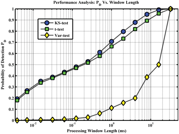
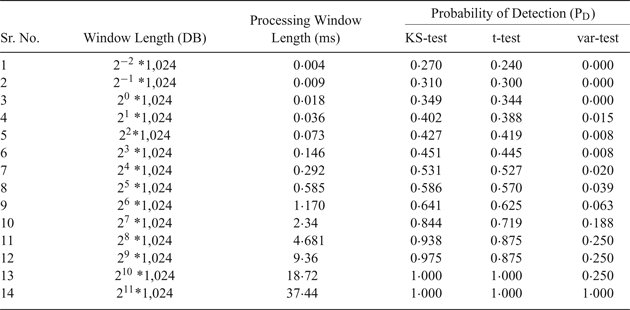
Table 5 shows the processing window length (DB) and the value of the PD obtained from different detection methods, as described in Section 2.4. The semi-logarithmic graph for the same is plotted by converting the window length in milliseconds (ms) using sampling frequency as shown in Table 4. As shown in Figure 14, it is clear that at the cost of more complexity, that is by increasing the processing window length, we get better performance for each detection method (Fadaei, Reference Fadaei2016). Also, the KS-test and t-test perform better than the var-test for each processing window length. In addition to that, a larger processing length (greater than 10 ms) provides rapid change in the performance of the var-test.
PD Vs. Processing window length for different detection methods.

Variable processing window length and PD for different detection methods.

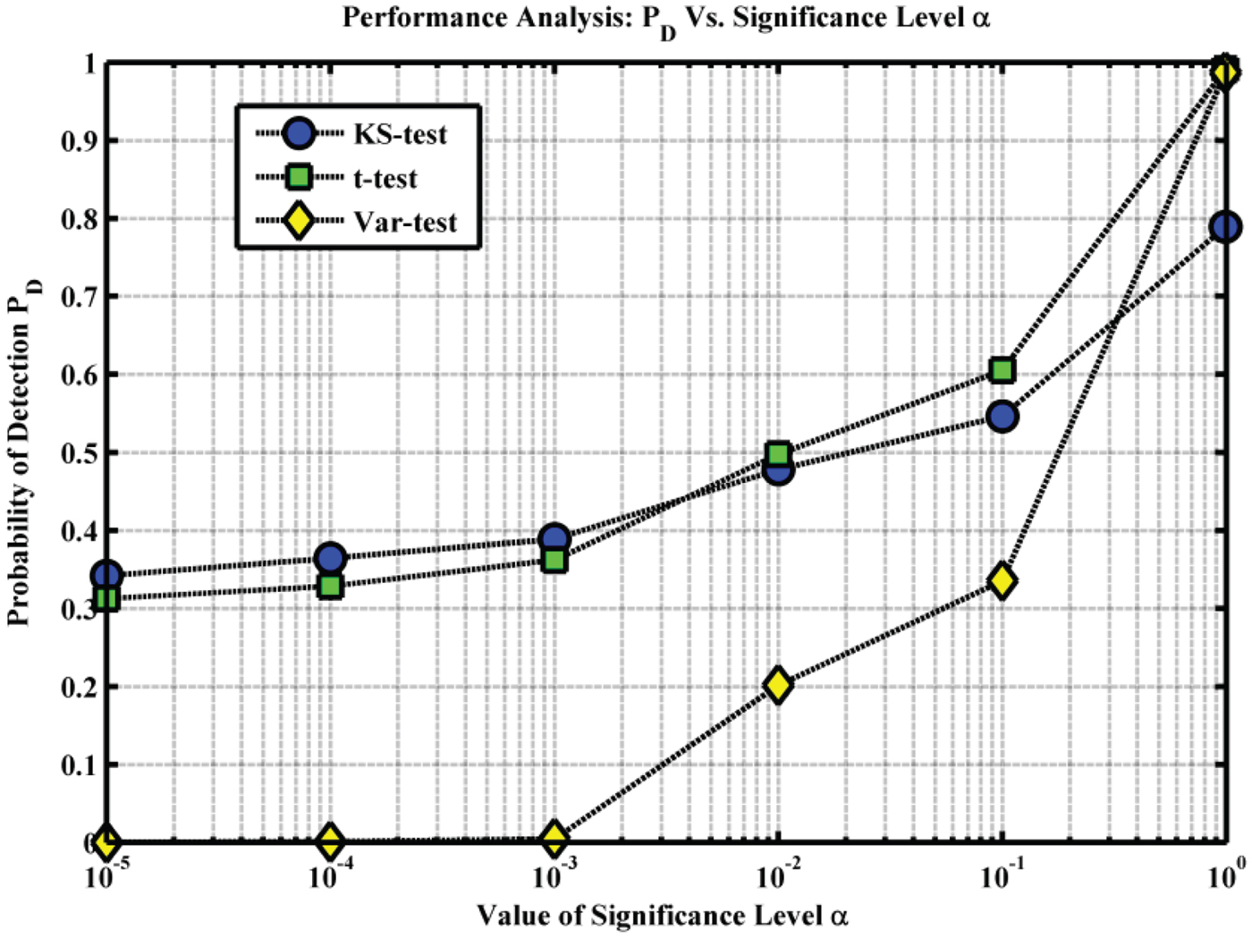
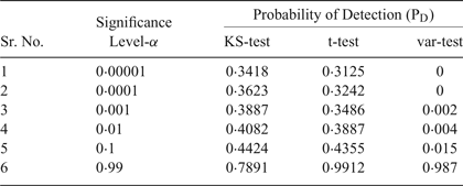
Table 6 provides the values of PD calculated with respect to changes in the value of significance level α for different detection methods. As can be seen from Figure 15, the KS-test and the t-test provide superior results for each value of α compared to the var-test method. Clearly, the var-test method has the worst performance, although for larger α (>0·05) it has improved performance over the KS-test and t-test.
PD versus significance level α for different detection methods.

Variable significance level α and PD for different detection methods

5. CONCLUSION
Various communication and electronic system bands or their harmonics may cause unintentional interference with NavIC signals. Here, Wi-Fi transmission produces interference to the S-band frequency of the NavIC, which was demonstrated by the simulation results of the PSD, acquisition performance and hypothesis testing. A drop in the performance of the NavIC receiver was observed, so these interfering signals need to be detected. To achieve optimal detection, design of an efficient detector in receivers is vital. The results were summarised by a detailed comparison of the p-value and decision analysis of the two-sample hypothesis tests. The performance curve of PD is consistent with the hypothesis analysis. In addition, it has been confirmed that the KS-test and the t-test methods require information of the interference-free population window but have almost the same performance and are superior to the var-test. So, the KS-test and the t-test are concluded to be more effective for detecting Wi-Fi interference. In the future, other threshold-based hypothesis detection methods can be investigated for the same interference case. Also, for reliable service of the receiver, Wi-Fi interference mitigation is vital. The analysis shown in this work may help to develop future mitigation methods for such types of RFI.
ACKNOWLEDGEMENTS
The authors would like to thank the scientists of SAC, ISRO for providing guidance and information about NavIC.