2. The dictator effect

This paper contributes to the larger debate about the effects of political institutions on economic performance. For the recent period, this debate has mainly focused on democratic regimes and their effects on economic growth (Barro, Reference Barro1996a; Chang, Reference Chang2011; Przeworski et al., Reference Przeworski, Alvarez, Cheibub and Limongi2000; Tavares and Wacziarg, Reference Tavares and Wacziarg2001). Rodrik (Reference Rodrik2002) for example argues that democracies produce more stable growth paths and are better at dealing with adverse shocks. Total factor productivity is also, according to Rivera-Batiz (Reference Rivera-Batiz2002), positively affected by the higher quality of institutions under democracy. Much of this literature assumes that democratization is a one-dimensional process–as measured by (for example) the PolityIV dataset. However, the literature on the economic effects of dictatorships is much more limited. This limitation can be explained by the enormous diversity the authoritarian regimes exhibit–from e.g. the North-Korean one-party-system to personalistic regimes in Africa dominated by ‘big men’ such as Mugabe or Mobutu. This wide diversity makes it much more difficult to generalize about the impact of authoritarian regimes on economic outcomes.

Nevertheless, two sets of papers considerably contributed to our understanding of dictators and their regimes. The first set can be found in the studies of McGuire and Olson (Reference McGuire and Olson1996) and Olson (Reference Olson1993), through which they developed a model that portrays the dictator as a ‘stationary bandit’, and the second set can be found in the work of Wintrobe (Reference Wintrobe1990, Reference Wintrobe1998), in which he developed a number of models covering different aspects of dictatorships. In the former set of papers, the basic idea of McGuire and Olson (Reference McGuire and Olson1996) and Olson (Reference Olson1993) is that dictators–even if they have unlimited power, which they are assumed to have in this approach–are constrained in their actions because increasing the level of taxation (or reducing spending on public goods) will have negative effects on the economy, and therefore, via taxation, on the income of the dictator. An absolute ruler, who is assumed to maximize his income via rent extraction, is therefore constrained by the Laffer curve effect. In short, “an ‘invisible’ hand gives a roving bandit an incentive to make himself a public-good-providing king” (McGuire and Olson, Reference McGuire and Olson1996: 71). In fact, the higher the tax rate, the more an autocrat will be interested in spending on public goods.Footnote ² There is however, one important qualification; the time horizon of the dictator has to be quite long to get this benevolent result. When his time horizon is short, he will not care anymore about the effects of increased taxation on economic growth; the discipline of the Laffer-curve will disappear, and he will become a ‘roving bandit’ who will plunder the economy.

The Olson-McGuire approach, however, assumes that dictators are economically rational and – even more problematic – have access to full information about the consequences of their choices in the long run. These assumptions have been criticized in the literature (Wintrobe, Reference Wintrobe1998). In his comprehensive and thorough analysis of dictatorships Wintrobe (Reference Wintrobe1990, Reference Wintrobe1998) was able to highlight the information problems faced by rulers of this kind. Given that dictators are the source of all power, people are reluctant to share their information with them, because the messenger of the bad news may well fall in disgrace. People will therefore tell the dictator what he wants to hear – and the dictator, knowing this, will not trust the information given to him by his assistants and ministers. This is Wintrobe's ‘dictator's dilemma’: since he is ‘almighty’, he will never know how loyal his entourage, let alone his subject population is, because they do not dare to signal disloyalty to him. A dictator is therefore caught in information asymmetries. People will try to flatter him by presenting too optimistic information about the state of the economy while suppressing the bad news, also because bad news may mean that they – as for example cabinet ministers – are not doing the expected good job. Once such a disinformation campaign has started, it is difficult to return to reality. The result of this ‘disinformation trap’ is that the president lacks a basis for sound economic decision making, which eventually will lead to adverse long term economic performance. Finally, a dictator has good reasons to distrust everybody: as Machiavelli famously remarked, a ruler is almost bound to die at the hands of somebody close to him.

There is a social-psychological dimension to the aforementioned dilemma as well. The experience of winning – of being ‘the strongest’, the one who successfully rose to power – will lead to the release of powerful drugs (testosterone, dopamine) in the brain, to which people may become addicted and which may change their behavior. Robertson (Reference Robertson2012) reviewed the various dimensions of this ‘winner-effect’, which makes those involved smarter and more focused, but also less emphatic and more egocentric, less open to outside criticism and poorer at decoding other people's emotions and expressions. Experiments with rats and mice have demonstrated that such addictions may even change the structure of the brain (Robertson, Reference Robertson2012). Such effects of power are well-known from social psychology. Powerful CEOs were, for example, more likely than business students to view other people as instruments of their own goals (Gruenfeld et al., Reference Gruenfeld, Inesi, Magee and Galinsky2008). Much of this research builds on Kipnis (Reference Kipnis1976) and Kipnis et al. (Reference Kipnis, Castell, Gergen and Mauch1976) ‘metamorphic model’ of the effects of power on behavior asserting that ‘through the repeated exercise of power individuals adopt more vainglorious self-concepts and as a consequence denigrate the less powerful’ (Keltner et al., Reference Keltner, Gruenfeld and Anderson2003: 266). Power also reduces inhibitions and increases the likelihood of socially inappropriate behavior – also because those in power become less sensitive to threat and punishment. Summing up, these studies confirm that power corrupts (Kipnis, Reference Kipnis1972).

This also has effects for the entourage of the powerful. Many dictators start their career as team players, leaders of a group of often military men who have staged a coup or won a contentious election. The logic of the dictator's dilemma and the winner-effect is that he will gradually eliminate other, more or less independent members of his team and increasingly rely on (for example) family members who are (in his view) more trustworthy or more willing to tell the ruler the stories he wants to hear. He may become increasingly lonely and paranoiac, and the quality of his (economic) decision making will decline accordingly.

The ‘dictator's dilemma’ can be solved in two ways: by repression or by loyalty/popularity – both are costly, however. Thus, “successful” dictators need a mix of repression and loyalty (or popularity) to survive in office, and this mix largely determines the character of the regime. Hence, it is possible to divide the authoritarian regimes into the following groups: 1. Military regimes, based on (following Mao's famous quote) ‘the barrel of the gun’ (high repression and low loyalty); 2. Monarchic/ Personalistic/Dynasty regimes, based on ‘traditional’ rule by a family (low repression and high loyalty); and 3. Single-Party/Totalitarian regimes, often based on ideology (communism), which makes possible the combination of high repression and high loyalty (Ellman, Reference Ellman2008; Geddes, Reference Geddes2003; Wright, Reference Wright2008). Similarly, Chang and Golden (Reference Chang and Golden2010) have analyzed the determinants of corruption in authoritarian polities and the effects that corruption has on growth in different autocratic regime types. Their results show that personalistic and personalistic-hybrid (monarchies) regimes are more prone to corruption than military and single-party ones, implying that rulers who have longer time horizons are less corrupt.

Authoritarian regimes may however be embedded in states with very different levels of institutionalization, often linked to the history of the state involved. The more rulers and their regimes are constrained by ‘independent’ bureaucracies and by institutions such as parties, legislatures and elections, the more durable they tend to be (Gandhi and Przeworski, Reference Gandhi and Przeworski2006), and the more balanced their economic policies will be (Boix, Reference Boix2003; Geddes, Reference Geddes1999). The best proxy for testing these constraints is probably the ‘antiquity’ of the state involved: in young African states with almost no traditions and checks and balances the freedom of action of an autocrat is clearly different from ‘ancient’ states that do have created such constraints (Putterman, Reference Putterman2007).

3. Data and variablesFootnote ³

In order to assess the ‘dictator effect’, we analyze annual data on economic, political and institutional variables for the period 1960–2009, for all countries that had a dictatorship for at least a four year time period. Given the restriction that we want to investigate the ‘dictator effect’, we had to exclude countries where no dictators ruled during this period. The outcome of this restriction was a sample of 100 countries located in Sub-Saharan Africa (45), Asia (21), Latin America (20) and the Near East (14). We used various sources to find out when and why a regime was classified as a dictatorship and, in turn, a leader as a dictator (Beck et al., Reference Beck, Clarke, Groff, Keefer and Walsh2001; Charron and Lapuente, Reference Charron and Lapuente2011; Geddes, Reference Geddes2003; Marshall and Jaggers, Reference Marshall and Jaggers2004; Przeworski et al., Reference Przeworski, Alvarez, Cheibub and Limongi2000; Teorell et al., Reference Teorell, Charron, Samanni, Holmberg and Rothstein2011). Our selection of dictators follows similar classifications as previous studies (Gandhi, Reference Gandhi2008; Goemans et al., Reference Goemans, Gleditsch and Chiozza2009; Wright, Reference Wright2008).Footnote ⁴ Hence, a country was included for the entire fifty-year period (1960–2009) only if it was ruled by a dictator for at least four years.Footnote ⁵

The dependent variables for the three different models are:

• • GDP per capita growth: data were taken from Penn World Table version 7 (PWT) (Heston and Summers, Reference Heston and Summers2011).

• • Quality of Political Institutions: data were taken from both the Polity IV project (Marshall and Jaggers, Reference Marshall and Jaggers2004) and the Vanhanen (Reference Vanhanen2011) dataset.Footnote ⁶

• • Inflation rate: data were taken from the World Development Indicators (World Bank, Reference World Bank2012)

The control variables used in the regressions as well as their expected outcome coefficients are:

• • Initial GDP per capita (log): log of real GDP per capita (taken from PWT), a negative coefficient is expected here because of the existence of conditional convergence across countries (Barro, Reference Barro1991; Sala-i-Martin, Reference Sala-i-Martin1994; Solow, Reference Solow1956).

• • Investment (percent of GDP): (taken from PWT) larger investment shares illustrate better economic performance, hence economic growth (Grabowski, Reference Grabowski2008; Mankiw et al., Reference Mankiw, Romer and Weil1992; Perotti, Reference Perotti1996). Thus, a positive coefficient is anticipated here.

• • Primary School enrollment (percent of population, gross): (taken from WDI) higher educational attainment indicates greater accumulation of human capital which, in turn, has been emphasized as a critical determinant of economic growth (Barro and Lee, Reference Barro and Lee2001; Mankiw et al., Reference Mankiw, Romer and Weil1992); hence, a positive correlation is expected between this variable and the dependent one.

• • Population growth: (taken from WDI) larger population growth will usually lead to lower GDP per capita growth rates. Thus, a negative relation is expected (Barro, Reference Barro1996b; Grier and Tullock, Reference Grier and Tullock1989).

• • Trade Openness (exports+imports/GDPpercapita,%): (taken from PWT) the literature suggests a strong positive effect of international trade on economic growth (Frankel and Romer, Reference Frankel and Romer1999; Rodriguez and Rodrik, Reference Rodriguez and Rodrik2001).

• • Share of Government in GDP (percent): (taken from PWT) various studies have demonstrated that a relatively large government is likely to be have adverse effects on economic growth due to inefficiency of government activities (Afonso and Furceri, Reference Afonso and Furceri2010), or due to restrictions on private investments (Bjørnskov et al., Reference Bjørnskov, Dreher and Fischer2007). Hence, a negative coefficient is expected.

• • Quality of Political Institutions: (taken from PolityIV and Vanhanen (Reference Vanhanen2011)) we acknowledge the fact that both datasets have their weaknesses (Munck and Verkuilen, Reference Munck and Verkuilen2002), therefore we have run each regression separately using both variables. The former intends to focus on the political constraints (constraints on the executive) and ranges from strongly autocratic (−10) to strongly democratic (10). The principal advantage of the index is that it examines concomitant qualities of democratic and autocratic authority in governing institutions, rather than discreet and mutually exclusive forms of governance. The polity variable provides a convenient avenue for examining general regime effects, therefore we include this variable to control for the quality of institutions in the baseline model. However, this index has been criticized by the Glaeser et al. (Reference Glaeser, La, Lopez-de-Silanes and Shleifer2004) paper, in which they argue that the Polity variables are highly volatile and do not reflect durable constraints on the executive, but political outcomes (2004: 7–9). The latter index is formed by a combination of two basic indicators of democratization; i.e. competition and participation. The degree of competition indicates the smaller parties’ share of the votes cast in parliamentary or presidential elections, or both. For example, if the largest party gets 40 percent of the votes, the share of the smaller parties is 60 percent. The degree of participation indicates the percentage of the population which actually voted in the same elections. These two indicators are combined to create the Index of Democratization which we use in the regressions. This index differs from the other measures of institutional quality in two crucial points: (1) it uses only two indicators (competition and participation) and (2) both of them are solely based on quantitative data. Two points that highlight at the same time the strength and weakness of this indicator. Nevertheless, many researchers have recognized and examined the importance of institutions on economic growth (Acemoglu, Reference Acemoglu2003; Glaeser et al., Reference Glaeser, La, Lopez-de-Silanes and Shleifer2004; Rodrik et al., Reference Rodrik, Subramanian and Trebbi2004; Ros, Reference Ros2011). Taking these studies into consideration a significant and positive correlation is expected between the quality of institutions and economic growth.

• • Religious fractionalization: Reflects probability that two randomly selected people from a given country will not belong to the same religious group. The higher the number, the more fractionalized society (taken from Alesina et al. (Reference Alesina, Devleeschauwer, Easterly, Kurlat and Wacziarg2003)). Scholars usually use ethnic, linguistic or religious fractionalization in order to capture social cohesion. Easterly et al. (Reference Easterly, Ritzen and Woolcock2006), argue that a higher level of homogeneity leads to a higher growth rate. However, Gandhi and Przeworski (Reference Gandhi and Przeworski2006) find that religious fractionalization is a stronger determinant of political and social cohesion in authoritarian regimes.Footnote ⁷ A negative sign is expected.

The key variable of the regressions is Years in Office (YRSOFFC), the number of years a ruler is in office since his rule began, taken from ACLP (Alvarez et al., Reference Alvarez, Cheibub, Limongi and Przeworski1996) combined with DPI dataset (Beck et al., Reference Beck, Clarke, Groff, Keefer and Walsh2001). The ACLP database's covers the period 1960–1994; the DPI dataset starts in 1975 and continues until 2010. Hence, the combination of these two databases allowed us to cover the whole period of interest; i.e. 1960–2009. The value of YRSOFFC increases each year when the leader remains in power, and starts at one again when a new ruler takes office.

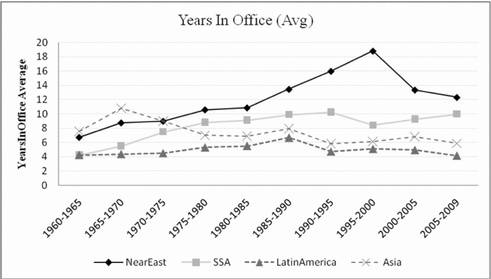
Figure 1 provides a graphic illustration of the evolution of the average years in office across the four different regions of the world included in this study. It seems that the remarkable high longevity of the dictators is to a large extend concentrated in Africa and in the Near East. Both of them show strong increases overtime; in Africa for instance, from a low of 4 years in 1960–1965 (partly due to their independence) to 10 years at present, and in the Near East from almost 7 in 1960–1965 to an amazing 19 in the 1995–2000 period, after which decline followed to 12 years in 2005–2009. Unlike them, Asia has the highest average in the 1960s and a declining trend is visible from 1970s onwards. Finally, Latin American countries do not seem to suffer from a similar trend of long lasting dictators, where the average remains around 5 years throughout the period of interest. A point which is confirmed by the econometric results (Table A-2, supplementary appendix).

Figure 1.

Years in office change over time.

Political scientists have studied the determinants of the years in office variable in order to explain why some rulers remained in power very long, whereas others were kicked out quickly (Acemoglu, Reference Acemoglu2006; Baker et al., Reference Baker, Bulte and Weisdorf2010; Geddes, Reference Geddes1999; Weingast and Wittman, Reference Weingast and Wittman2008). Rulers leave office in many ways. Some of them die while in office by natural causes, sometimes to be succeeded by their sons. This is usually the case in monarchies. Some are deposed by a popular revolution, like Gaddafi in Libya. Military dictators usually are overthrown by another coup. According to Geddes (Reference Geddes1999) the probability to oust a dictator rises in the first two decades because of the economic shocks, scandals and corruption, and then decreases over the next periods. Then, after 35 years in office the likelihood of regime breakdown starts increasing again. This is however not confirmed by our data, which show a log-linear distribution of years in office, which points to stability in the chance to end rule (Figure A-1, supplementary appendix).

Finally, we use a number of classifications of states and regimes in order to further explore the relationship between economic growth and years in office. We try to investigate how varying determinants, for instance different regime types, impact on the outcome of the dictator effect. Do they mitigate it? Do they increase the explanatory power of the model? Therefore, three different sets of interaction terms were included in the regressions:

• • we coded three types of authoritarian regimes following Geddes (Reference Geddes2003) and Wright (Reference Wright2008) in order to examine the different effects that each type of autocracy has on economic growth. We created separate dummies for the three different regimes: military, monarchy and single-party. The interaction term between the regime dummy and the Years in Office variable was then entered in the regression to find out what effect different regimes had on economic performance.

• • we investigate whether state antiquity interacted with years in office has an effect on economic growth; in young states, such as almost all Sub-Saharan countries, without a certain institutionalization of power will probably be more ‘personalistic’, implying that the ‘dictator effect’ is stronger there; ‘old’ states, such as Egypt, or Ethiopia, may have developed stronger institutions to constrain the power of the executive; we used the “State Antiquity Index” (Putterman, Reference Putterman2007) to measure this effect, but divided the sample of countries into two groups, the young states (independent since the 1960s) and the older states (and created a dummy to the latter states).

• • another obvious factor that we would like to include in the analysis is whether a country is oil producing or not;Footnote ⁸ the Olson model assumes that a dictator is constrained by the Laffer curve effect (Laffer, Reference Laffer2004), but once oil – or another, similar natural resource – enters the picture a ruler can simply extract his rents from this the proceeds of oil, without hurting the economy very much (Wright, Reference Wright2008).Therefore we identified the oil producing countries (see classification table, Appendix (C)), and analyze the interaction between ‘oil’ and Years in Office.

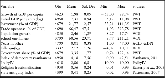
Descriptive statistics of the variables used in the baseline and extended model are illustrated in the following table (see Table 1). These statistics can provide the context in which to assess the magnitudes of the econometric results.

Table 1.

Descriptive statistics

There is, apart from the protests during the Arabic Spring, some prima facie evidence that dictators, who stay in office for a long time, may have a poor economic record. If we set out the ‘years in office’ of the dictators of a number of African countries against the development of their GDP per capita we get a picture as presented in Figure A-2, online appendix. Most dictators do rather well during the first part of their tenure (although in the case of Libya this was perhaps sheer luck: the oil crisis of the 1970s improved things a lot for the country). But after a while, the economy of these countries began to go down: GDP per capita declined dramatically in all four of them. This was also independent of the year in which they took office, because the four countries of Figure A-2 were selected such that the start of these regimes was spread in time (Ivory Coast's HoupHouët Boigny: 1960; Zaire's Mobutu: 1965; Libya's Gadaffi: 1969 and Zimbabwe's Mugabe: 1980). Only Gadaffi managed to turn his economy around after a disastrous slide during the 1980s and 1990s, but this was mainly due to oil exports and high oil prices. Moreover, the level of real income remained quite low compared to the situation of Libya when he seized power: its GDP per capita in 2008 was only a third of the level of the mid-1960s. This example also demonstrates how important oil may have been for the countries concerned – we therefore also look at this factor in our regressions.

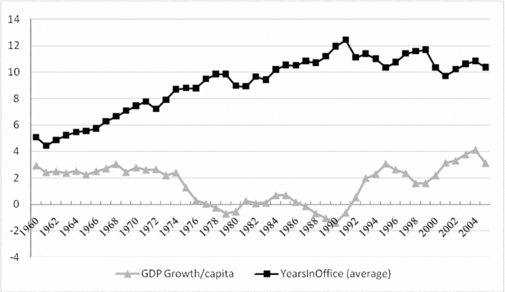
Turning to economic growth, Figure 2 shows the average per year value of the YRSOFFC variable scatter-plotted with average per year GDP per capita growth. After independence, in the early 1960s, the average YRSOFFC value obviously started at a relatively low level, but it increased until the early 1990s when the average ruler was in office for about 12 years. It has slightly declined since then – obviously the democratic wave of the 1990s did have some impact on it (Bratton et al., Reference Bratton, Van de Walle and Lange1997) – but on average the decline is quite small (to 11 years in 2009). Figure 2, provides a good illustration about the connection we are trying to establish: long years in office do seem to be correlated with slow economic growth.

Figure 2.

Average value of years in office and the average rate of growth, 1960–2009.

4. The method

This section explains the empirical method we follow in our attempt to assess the ‘dictator effect’ on the three different indicators that we described above. We first estimate the link with GDP per capita growth and, in order to help explain the patterns found, we next examine if years in office also affect inflation and the quality of democratic institutions. Over the last few years several important advances have been occurred in the empirical literature of economic growth. This is due to new, more sophisticated panel data methods emerging to solve the econometric difficulties that growth researchers have faced. The panel data method that currently appears to be the most efficient is the generalized method of moments (GMM) developed by Bond et al. (Reference Bond, Hoeffler and Temple2001). The advantage of this method is that it takes account of the time series dimension of the data, the non-observable country specific effects, the inclusion of a lagged dependent variable among the explanatory variables, and the possibility that all explanatory variables are endogenous (Roodman, Reference Roodman2006; Vieira et al., Reference Vieira, MacDonald and Damasceno2012). Thus, throughout this paper, we employ the system-GMM estimator.

The empirical model for economic growth can be summarized as follows:

(1)\begin{equation} \begin{array}{l} \Delta Y_{{\rm it}} = \gamma Y_{i,t - 1} + \beta X'_{{\rm it}} + \delta Z'_{{\rm it}} + \nu _\iota + \mu _t + \varepsilon _{{\rm it}} \\ i = 1, \ldots ,N\;{\rm and}\;t = 1, \ldots ,T \\ \end{array}\end{equation}

where ΔY _it is the log difference in per capita GDP (i.e. economic growth), Y_{i ,t-1} is the logarithm of per capita GDP at the start of the period (initial GDP per capita), X′_it is a vector of economic determinants of economic growth, Z′_it is a set of control variables (both political and institutional ones) measured during the period. ν_ι controls for all time-invariant country fixed effects and μ_t controls for factors that may affect levels of economic growth across countries at the same year, and ε_it is the error term.

Most scholars use a five-year average time period in order to address their hypothesis. They argue the dynamic panel model is designed for less time periods (T) than cross sections (N) in order to control for dynamic panel bias (Arellano and Bond, Reference Arellano and Bond1991). However, Hayakawa (Reference Hayakawa2012) argues that even though system-GMM was originally developed for relative small T and large N, the two step system-GMM estimator, which is our case, has consistency and supports large time and cross section dimensions. Therefore, annual data were used to investigate the main hypothesis.Footnote ⁹

Since most of the explanatory variables can be affected by economic growth and raise concerns of endogeneity, all of the variables are treated as endogenous ones. We use lagged levels of these variables as instruments for the current differences—lagged two or more periods, and their once lagged first-differences in the levels equation, in order to control for any potential endogeneity and to avoid reverse causality bias. This is a standard procedure in the empirical literature (Aisen and Veiga, Reference Aisen and Veiga2013; Dreher, Reference Dreher2006; Jong-A-Pin, Reference Jong-A-Pin2009). An important and common mistake that growth scholars make is that they fall into the trap of generating too many instruments, which is called the instrument proliferation problem (Roodman, Reference Roodman2009). Numerous instruments may seem individually valid, but can be collectively invalid because they overfit endogenous variables. Therefore, Mehrhoff (Reference Mehrhoff2009) and Roodman (Reference Roodman2009) offer a solution to control and limit the number of instruments in order to get consistent estimates. Even though they both agree that there are no clear rules for the exact number of lags and instruments in the estimator, they propose two techniques to reduce the instrument count and obtain reliable results. One of them is by limiting the lag depth and the other one is by “collapsing” the instrument set. They strongly recommend to the researchers not to use more instruments than observations and to check whether the Hansen J-statistic indicates a perfect p-value of 1.00, which should not be the case. Thus, in the tables presenting our results we mention all the above diagnostic tests. Finally, we use Windmeijer (Reference Windmeijer2005) finite sample correction of standard errors in order to increase robustness.

5. Empirical results

(A) Years in office and economic growth

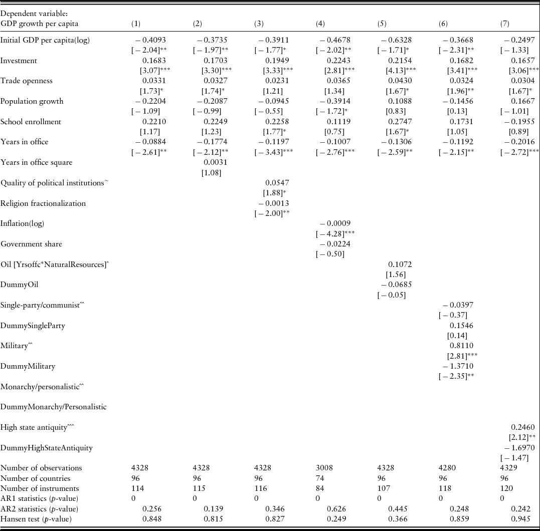
The main testable hypothesis is the following: does long tenure affect economic growth? Is there, more generally, a relationship between years in office of rulers and economic performance? Table 2 presents the first set of results. Firstly, we estimated the baseline model in column (1). The years in office variable is highly statistically significant and adversely affects economic growth. This correlation implies that when there is an additional year in office by the same leader, the annual growth rate decreases by 0.088%, after 20 years of rule the dictator depresses growth by more than 1.77% per year. The control variables yield the expected signs and confirm our expectations: initial GDP per capita is negatively correlated with growth; investment and trade openness have a positive effect on growth and both appear to be significant. Population growth does have the expected negative coefficient, although it is not statistically significant, and, finally, school enrollment has a small positive effect (depending on the specification significant or not).Footnote ¹⁰ In column (2) we include the square term of yrsoffc (YRSOFFCSQ),Footnote ¹¹ which we created to examine if the relationship was linear or not.Footnote ¹² However, the results verify that there is not a non-linear relationship between YRSOFFC and economic growth.Footnote ¹³

Table 2.

Years in office and economic growth

Notes: ^(a)System GMM estimation for dynamic panel data-model. Sample period: 1960–2009.

^(b)Corrected T-statistics are in brackets. Significance level at which the null hypothesis is rejected: ***, 1 percent; **, 5 percent, and *, 10 percent.

^(c)Second (and latter) lags were used as instruments in the first-differenced equations and their once-lagged first differences were used in the levels equation.

^(d)Two-step results using robust standard errors corrected for finite samples (using Windmeijer's correction (Reference Windmeijer2005)) Time dummies are included in all regressions.

^(e)(~) In the regressions both variables of institutional quality have been included separately. In this table we only present the Index of Democracy from Vanhanen (Reference Vanhanen2011).

^(f)(^) We constructed two interaction terms to capture the effects that each region multiplied by the years in office variable has on economic growth with respect to oil production. Those interaction terms, such as oil countries and non-oil countries are created out of one continuous variable (YRSOFFC) and one dummy variable (REGION*).

^(g)(^^) We constructed three interaction terms to capture the effects that different types of regimes multiplied by the years in office variable have on economic growth. Those interaction terms, such as Single Party/Communist, Monarchy/Personalistic and Military are created out of one continuous variable (YRSOFFC) and one dummy variable (REGIME*).

^(h)(^^^) We constructed two interaction terms to capture the effects that the state antiquity index multiplied by the years in office have on economic growth. Those interaction terms, such as Low and High Antiquity are created out of one continuous variable (YRSOFFC) and one dummy variable (STATEHIST*).

In column (3) we added a proxy for the quality of institutions, i.e. index of democracy by Vanhanen (Reference Vanhanen2011),Footnote ¹⁴ and the index of religious fractionalization. The results show that the quality of political institutions has a positive and significant effect on growth, even though it is only statistically significant at a 10% significance level. Nevertheless, this gives support to the institutionalist literature supporting that more democratic institutions enhance economic growth. Additionally, Religious fractionalization variable yields the expected negative coefficient and is statistically significant, confirming previous findings by Easterly et al. (Reference Easterly, Ritzen and Woolcock2006). Nevertheless, the coefficient of YRSOFFC is not really affected by adding these variables; it is reassuring that this coefficient became slightly larger and more significant. Column (4) shows similar results after adding macro-economic stability variables; inflation (log) has a statistically significant negative coefficient, the share of government in GDP does not seem to affect growth.

Next, we interacted YRSOFFC with an oil-dummy to find out if the effect presented before can be found in both oil and non-oil producing countries (column 5). The results suggest that in oil producing countries long tenure does not seem to impact that much (the coefficient of the interaction term is positive but insignificant), which is probably explained by the fact that the state is not dependent on extracting rents from the indigenous economy.Footnote ¹⁵ What perhaps also plays a role is that the ups and downs of oil producing countries are so much determined by the big swings in oil production and prices, that domestic-political matters do not seem to have much of an impact on the economy.Footnote ¹⁶

Second, several political scientists have argued that varying regimes impact considerably different on the economy (Gandhi, Reference Gandhi2008; Geddes, Reference Geddes2003; Wintrobe, Reference Wintrobe1990, Reference Wintrobe1998; Wright, Reference Wright2008). Hence, a question arises from these previous findings; does ‘the dictator effect’ impact similarly on different authoritarian regimes? Column (6) of Table 2 shows that the kind of regime did not matter considerably: only military regimes do not seem to suffer, in relative terms, from the ‘dictator effect’, because the interaction effect is positive and compensates for the negative effect of the YRSOFFC variable. However the military-dummy is strongly negative, suggesting a depressing effect on growth independent of years in office. Finally, the estimated coefficients of the constructed interaction terms with the State Antiquity Index (Putterman, Reference Putterman2007) are reported in the last column. The idea was that younger states are more plagued by the dictator effect than old ones. This is confirmed: the interaction term of high state antiquity and years in office has a positive coefficient that compensates the negative coefficient of YRSOFFC. Apparently, the ‘dictator effect’ is a problem of young states.

(b) Robustness tests/alternative explorations

Several robustness tests were performed with the purpose of checking whether the empirical results, indicating adverse effects of years in office on economic growth, remain significant and reliable. First, we test whether the results are driven by the selected econometric specification (i.e. the system-GMM). Hence, we ran the same regressions of the same model with OLS, which basically produce the same results – a consistent negative YRSOFFC coefficient of about the same magnitude.

Second, we examine if the “steady-state” assumption holds as suggested by Roodman (Reference Roodman2009). He argues that this check can be used to examine the validity of the instruments used in the system-GMM estimator. In other words, the estimated coefficient of the lagged dependent variable in all our models should be less than unity, indicating convergence; otherwise the GMM estimator is invalid. Bond (Reference Bond2002) argues that additional checks for the dynamic panel estimate's validity can be made, by regressing the same model in a different specification, i.e. Ordinarily Least Squares (OLS) and Fixed Effects (FE) estimators. The estimated coefficient of system-GMM should lie between those two; something that holds in our case (results are not reported).

Third, we examine whether the link between economic growth and years in office changed over time. To achieve that, we divided the sample into two periods, 1960–1991 and 1992–2009. The purpose behind this division is twofold: (a) the period of the Cold War, before the final disintegration of the USSR in 1991, and (b) the wave of democratic change/transition in Africa and Europe during the 1990s. We find a sizable negative effect in both periods; the coefficient of YRSOFFC did decline a bit however (Table A-1, column 1&2).

Fourth, when we, instead of taking annual observations, convert all variables into (non-overlapping) five-year averages, we again get results which are very close to the baseline model; years in office variable has a strong negative link with economic growth, but the coefficient is somewhat smaller here (Table A-1, columns 3–6). To sum up, there is enough evidence to suggest that our findings for the ‘dictator effect’ are quite strong.

Alternatively, as it is illustrated in Table A-2, we investigate whether there is a different regional ‘dictator effect’ on economic growth, by adding dummy variables and interaction terms into the regressions. The effects are striking. At first, in column 1, the regional dummy variables do not add any additional explanatory value to the model; apparently, there are no significant regional patterns in per capita growth. However, when the region dummies are interacted with YRSOFFC in column 2, they have a considerable effect: SSA and Near East countries seem to suffer remarkably more from the ‘dictator effect’. This effect even increases when quality of institutions is also taken into account (column 3). On the other hand, the coefficient for Latin America (the reference category in these regressions) is positive and insignificant.

It is important to note here that the net ‘dictator effect’ in Asia is driven by the statistical significance effect of its dummy variable, which is 0.0358 and after calculations one can see that the net ‘dictator effect’ of Asian countries (coefficient: −0.1360 and p-value: −1.92) is statistically significant at 10% significance level. This does not imply that the ‘dictator effect’ is absent in this part of the world, rather that the Asian and Latin American countries are less affected, in relative terms, as compared to the ones in Sub-Saharan Africa and the Middle East. To shed more light on the varying regional effects, we divided our dataset in 3 different sub-samples (Latin America, Asia and Sub-Sahara Africa/Middle-East) and re-estimated the model. The results show that all regions suffer, to various degrees, by the ‘dictator effect’(see Table A-4). Finally, the estimated coefficients in column 4 did not alter significantly when we controlled for any macroeconomic stability (inflation & government share) and state antiquity effect. It is worth noting here, that the state antiquity index by itself does not exhibit explanatory power to the model, and hence, does not account for cross-country growth variations. It only adds explanatory value when it is interacted with the YRSOFFC variable (see Table 2, column 7).

(B) Years in office and institutions

Good governance is now generally considered to be a driver of economic development. We already saw that the regressions presented so far suggest that there is a negative correlation between economic growth and the years in office variable. We now want to investigate the impact of the ‘dictator effect’ on the quality of democratic institutions, measured by the Vanhanen (Reference Vanhanen2011) dataset and by the PolityIV variable. Many studies describe the effects of authoritarian regimes on state capacity and the quality of government (Charron and Lapuente, Reference Charron and Lapuente2011; Geddes, Reference Geddes2003; Wintrobe, Reference Wintrobe1990, Reference Wintrobe1998; Wright, Reference Wright2008). For instance, Charron and Lapuente (Reference Charron and Lapuente2011), investigated the differential impact of those regimes on the quality of government and identified the mechanisms through which different authoritarian rulers (such as military, monarchy and civilian) affect the quality of government. Our results provide considerable support to their theoretical reasoning, that single-party regimes are more responsive to citizens’ demands than the other two types of authoritarian rule because they have a structured mechanism to channel citizens’ “voices” (Table 3, column 3).

Table 3.

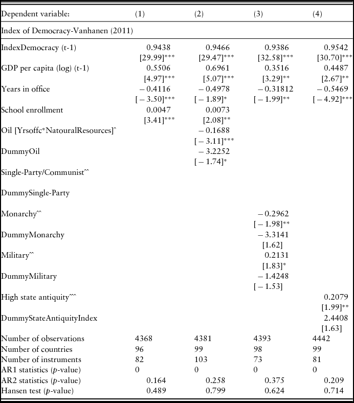
Institutions and years in office

Notes: ^(a)System GMM estimation for dynamic panel data-model. Sample period: 1960–2009.

^(b)Corrected T-statistics are in brackets. Significance level at which the null hypothesis is rejected: ***, 1 percent; **, 5 percent, and *, 10 percent.

^(c)Second (and latter) lags were used as instruments in the first-differenced equations and their once-lagged first differences were used in the levels equation.

^(d)Two-step results using robust standard errors corrected for finite samples (using Windmeijer's correction (Reference Windmeijer2005)). Time dummies are included in all regressions.

Figure A-3a & A-3b, in the online appendix, show the patterns that we are trying to explain, the development of the weighted average of the PolityIV variable (in this figure rescaled to 0 to 20) and the similar graphs based on the Vanhanen dataset (Reference Vanhanen2011). These two independent measures of the quality of political institutions show very similar patterns, which is reassuring: Latin America is the most democratic region, especially from the mid-1980s onwards, whereas the Middle East has on average the lowest scores. Both datasets show a moderate decline during the 1960s and 1970s, and much progress in democratic institutions from the mid-1980s onwards. But there are also clear differences, such as the decline in Middle-eastern scores in recent years in the Vanhanen which are not paralleled by the PolityIV data, which, given the problems with these kind of data, imply that the best strategy is probably to use both and compare the results.Footnote ¹⁷

Does long tenure of a ruler have an effect on the quality of institutions? One would expect that the logic explaining the effect of years in office on growth would result in a similar causal link between long tenure and institutional quality. The question is: how could one model the determinants of the democratic quality of institutions? There is obviously a link with GDP per capita (Acemoglu et al., Reference Acemoglu, Johnson, Robinson, Anghion and Durlauf2005; Rodrik et al., Reference Rodrik, Subramanian and Trebbi2004; Sachs, Reference Sachs2003). Moreover, institutions are relatively stable, which is also clear from a visual inspection of the Democratization Index (Vanhanen, Reference Vanhanen2011) as well as of the PolityIV dataset: usually the quality of institutions does not change from year to year. So including the lagged of the dependent variable makes it possible to concentrate on changes only. Taking into consideration previous findings, we begin by considering the following dynamic framework which is common practice now in the growth and institutional literature (Levine et al., Reference Levine, Loayza and Beck2000). Hence, the econometric linear regression model can be summarized as follows:

(2)\begin{equation} D_{i,t} = \alpha D_{i,t - 1} + \gamma Y_{i,t - 1} + X'_{i,t - 1} \beta + \mu _t + \delta _\iota + u_{{\rm it}}\end{equation}

where D_{i ,t} is an index of the quality of institutions in country i in period t. The lagged value of the dependent variable (D_{i ,t-1}) is included to capture the persistence in the quality of institutions and also the slow change in the political structure of a country. Moreover, Y_{i ,t-1} is a proxy for economic development such as the one period lag of GDP per capita (log).Footnote ¹⁸ Therefore, the parameter γ measures the effect of GDP per capita on democracy. In addition, μ_t and δ_i are respectively time-specific and country-specific effects. Finally, other institutional or political variables are captured by the vector X′_{i, t − 1.}

Since it is once again a dynamic panel data model, the OLS (either fixed or random effect) specification is unreliable. Therefore, the system-GMM estimator is also preferred in this case. In Table 3 the results are reported using the Vanhanen data (Democratization Index) as the dependent variable.Footnote ¹⁹ As expected, there is strong persistence; GDP per capita (log) and school enrollment both contribute to higher levels of institutional quality. Years in office has a strong negative effect on the Democratization Index: 20–25 years in office imply a lowering of the variable with about ten units, which given the scale from 0 to 42 is quite sizeable.Footnote ²⁰

The institutions of both oil and non-oil-producing countries are negatively affected by long tenure, but the effect for oil-producing countries is larger, confirming the resource curse literature that stresses the negative effect of oil on governance (column 2). The interaction term of YRSOFFC with regime types (column 3) imply a strong negative effect induced by the monarchic regimes, when compared with the communist/single-party ones. This result corroborates previous findings by Charron and Lapuente (Reference Charron and Lapuente2011) who argue that some types of dictatorship (i.e. single-party) produce higher quality of government than others (i.e. monarchy and military). A crucial point stemming from this result is that monarchic regimes are more detrimental for the development of democratic institutions over time. Finally, we again find that especially young states suffer from the ‘dictator effect’– the consequences in this case, are felt through the deterioration of democratic institutions.

(C) Years in office and inflation

One of the most ‘convenient’ ways for a ruler to acquire rents from a country is via the printing press. But printing money will result in inflation, which is therefore not only a proxy of ‘rent extraction’ by the state (McChesney, Reference McChesney1997), but it has also been linked to national socio-economic conflict (Collier and Hoeffler, Reference Collier and Hoeffler2005) –if unions are strong they will demand higher wages, resulting in a wage-price-spiral (Blanchard, Reference Blanchard1986). We expect that inflationary pressures will build up with years in office, which appear to be confirmed by a first look at the data. Figure A-5, online appendix, presents a selection of dictators (Mugabe in Zimbabwe, Jawara in Gambia, Stevens in Sierra Leone and Mobutu in Zaire) and their track record in terms of inflation (in log-scale). In all four cases there is a clear upward trend – the data on Zimbabwe even end after 27 years because inflation went through the roof.

The objective of this section is to investigate the effects of long tenure on inflation levels. This is done by estimating a dynamic panel data model for annual inflation levels. In order to avoid the high variability problem, which inflation in those countries exhibit, we use the logarithm of inflation as the dependent variable.

The empirical inflation model can be summarized as follows:

(3)\begin{equation} \begin{array}{l} (\log )\;{\rm Inflation}_{i,t} = \alpha (\log )\;{\rm Inflation}_{i.t - 1} + X'_{i,t} \beta + W'_{i,t\gamma } + \delta _i + \mu _t + u_{i,t} \\ i = 1, \ldots ,N\quad t = 1, \ldots ,T_i \\ \end{array}\end{equation}

where X′_{i, t} is a vector of strictly exogenous variables and W′_{i, t} a vector of endogenous covariates, μ_t and δ_i are time-specific and country-specific effects respectively, and u_{i ,t} is the error therm.

It has been argued that one determinant that could explain different inflation outcomes across countries is the occurrence of crisis at the government level (Aisen and Veiga, Reference Aisen and Veiga2006); therefore we use a relevant variable taken from CNTS to capture this effect and avoid omitted variable bias issues.

• • Government Crises (taken from CNTS): indicates any rapidly developing situation that threatens to bring the downfall of the present regime, excluding situations of revolt aimed at such overthrow. We expect this variable to have a positive and significant coefficient on inflation.

Political scientists have long argued about the existence of political business cycles (Nordhaus, Reference Nordhaus1975; Rogoff, Reference Rogoff1990). This literature predicts that opportunistic policy making is particularly likely to occur in the run-up to elections. It has been demonstrated that incumbents induce good economic conditions just before an election in order to stay in power. Myopic voters, as Nordhaus (Reference Nordhaus1975) first named them in his seminal paper, have the tendency to observe the current performance of the incumbent instead of the incumbent's policies throughout his years in office. Therefore, just before elections the incumbent uses monetary and fiscal policies (well-known Phillips curve effect) to manipulate the economy to win more votes (Martinez, Reference Martinez2009).

The existence of political business cycles has been investigated by economists and political scientists, primarily in the context of developed democracies (Alesina, Reference Alesina1997; Block, Reference Block2002; Shi and Svensson, Reference Shi and Svensson2006). These cycles predict that inflation may decrease prior to elections, but will increase with a lag the following year. Cases such as the Sub-Saharan Africa or other nascent democracies provide fertile ground for investigation, where voters in these regions are easier manipulated due to lack of information, and leaders act more opportunistic, relatively to what is happening in well-established democracies. Hence many dictators, in their attempt to stay in power, usually go to elections in an institutional environment more favorable to them than to their challengers. Decisions on fiscal policies are highly centralized in rulers’ hands and monetary authority is also often strictly controlled by them. Therefore, they can unrestrictedly expand the money supply in the year prior to elections, for instance, to temporarily increase employment.

As Bratton et al. (Reference Bratton, Van de Walle and Lange1997: 63) pinpoint, the political power is systematically concentrated in the hands of one individual, who resists delegating all but the most trivial decision-making tasks. Consequently, in our analysis we chose to include presidential elections where the impact might be stronger. For instance, between the early 1990s and 2009, more than 100 presidential elections involving more than one candidate were held in sub-Saharan Africa. It is expected that presidential elections in the following year will have a negative -temporary though significant- impact on inflation rates. A potential significant PBC-effect through elections, may pinpoint the increased importance of elections in the politics of these regions. Therefore, to control for this effect on inflation we use the following variable:

• • Elections (taken from CNTS): elections held for the presidency in a given year.Footnote ²¹

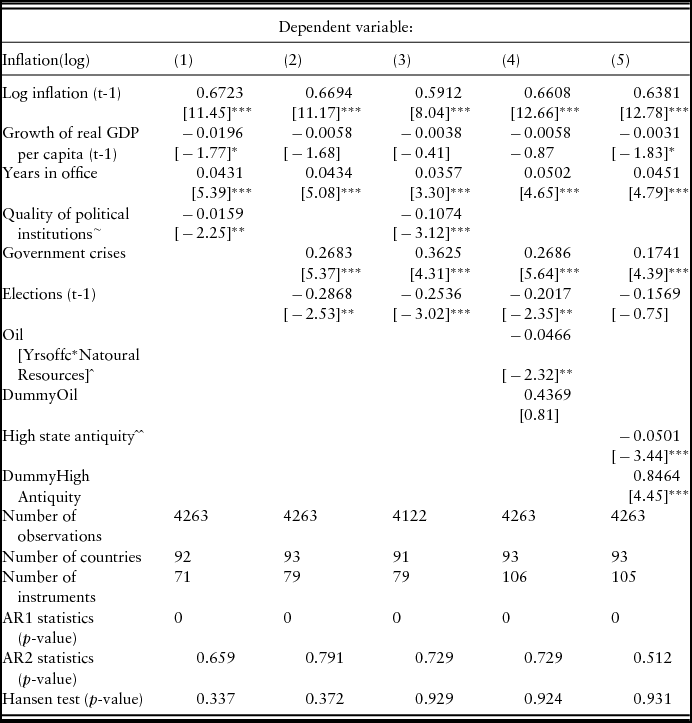
The results of the regressions shown in Table 4, point to a strong positive effect of years in office on inflation. The quality of democratic institutions is as expected negatively linked to inflation (column 1&3). We also find that elections in the previous year (t-1) have a dampening effect on inflation, pointing to a PBC effect. In order to add reliability to the finding, we also tested if elections in the same year (t) affect inflation, but could not find a significant result. However, when we included elections in the following year (t+1) the variable becomes significant again and this time, positively associated with inflation rates, confirming our hypothesis (results are not reported). Moreover, including elections in the growth regressions did not produce any significant result, an outcome which suggests that it is much easier for a dictator to manipulate inflation rates (and fiscal policies in general) than GDP per capita growth. Oil producing countries are less affected by the years-in-office-effect (column 4). Finally, it appears that young states show this link between tenure and inflation more consistently than old states (column 5).

Table 4.

Inflation and years in office

Notes: ^(a)System GMM estimation for dynamic panel data-model. Sample period: 1960–2009.

^(b)Corrected T-statistics are in brackets. Significance level at which the null hypothesis is rejected: ***, 1 percent; **, 5 percent, and *, 10 percent.

^(c)Second (and latter) lags were used as instruments in the first-differenced equations and their once-lagged first differences were used in the levels equation.

^(d)Two-step results using robust standard errors corrected for finite samples (using Windmeijer's correction (Reference Windmeijer2005)) Time dummies are included in all regressions.

^(e)(~) In the regressions both variables of institutional quality have been included separately. In this table we only present the Index of Democracy from Vanhanen (Reference Vanhanen2011).