1 Introduction
The deposition of a drop onto a film of the same liquid is an important process in applications ranging from spray painting (Cormier et al. Reference Cormier, McGraw, Salez, Raphaël and Dalnoki-Veress2012) and ink-jet printing of solution-processed organic electronics (Thompson et al. Reference Thompson, Tipton, Juel, Hazel and Dowling2014), on the microscale, to the 3D printing of food (Godoi, Prakash & Bhandari Reference Godoi, Prakash and Bhandari2016), on the macroscale. In spray painting, a film is rapidly formed through the coalescence of the first few droplets impacting an initially dry surface, so that subsequent drops spread on a liquid layer whose thickness increases with the deposited volume. Similarly, the manufacture of organic electronics relies on the sequential deposition of partially overlapping microdroplets which coalesce upon impact and spread due to capillary pressure differences to form a liquid line (and eventually a solid film after evaporation of the solvent). By contrast, in food printing, the larger deposited volumes tend to spread due to gravity. In this paper, we investigate the effect of the thickness of the underlying liquid film on the spreading of both ‘small’ and ‘large’ drops using a combination of experiments, numerical modelling and scaling analyses.
While the spreading of droplets on an existing layer of fluid is of interest in its own right, much previous work on this problem has been motivated by the fact that the presence of a thin precursor film regularises the contact line singularity that arises when a drop spreads on a perfectly dry substrate; see, e.g. de Gennes (Reference de Gennes1985), Yarin (Reference Yarin2006), Bonn et al. (Reference Bonn, Eggers, Indekeu, Meunier and Rolley2009), Samsonov (Reference Samsonov2011), Popescu et al. (Reference Popescu, Oshanin, Dietrich and Cazabat2012) and Snoeijer & Andreotti (Reference Snoeijer and Andreotti2013). The existence of such films was confirmed in early experiments by Quincke (Reference Quincke1877) and Hardy (Reference Hardy1919). Nanoscale liquid polymer droplets spreading on thin films of the same fluid have been studied computationally (Milchev & Binder (Reference Milchev and Binder2002), Heine, Grest & Webb III (Reference Heine, Grest and Webb2003); see also Pierce, Perahia & Grest (Reference Pierce, Perahia and Grest2009) for spreading on permeable surfaces). The thickness of the precursor films tends to be in the range from
 $h_{\infty }=10$
to 100 nm (Kavehpour, Ovryn & McKinley Reference Kavehpour, Ovryn and McKinley2003). This is much thinner than the films we consider in the current study within which we focus on a regime in which the spreading is driven by gravity and/or surface tension, with gravity dominating for ‘large’ drops and surface tension dominating for ‘small’ ones. We aim to characterise the spreading of such drops and to contrast their behaviour to that observed when they spread on dry substrates.
On dry substrates, drops of partially wetting fluids evolve towards their sessile equilibrium configuration which is parametrised by the finite equilibrium contact angle between the liquid and solid substrate. As the equilibrium contact angle approaches zero the drops become perfectly wetting and continue to spread indefinitely. Tanner (Reference Tanner1979) analysed this scenario using a thin-film model and showed that for ‘small’ drops whose motion is driven by a balance of capillary and viscous forces, the drop height,
 $H(t)$
, and radius,
 $R(t)$
, ultimately display a power-law behaviour, with
 $H(t)\propto t^{-1/5}$
and
 $R(t)\propto t^{1/10}$
, respectively. Lopez, Miller & Ruckenstein (Reference Lopez, Miller and Ruckenstein1976) and Huppert (Reference Huppert1982) considered the case of ‘large’ drops whose motion is driven by a balance of gravity and viscous forces. They showed that in this regime, the large-time behaviour is again described by power laws but with different exponents, namely
 $H(t)\propto t^{-1/4}$
and
 $R(t)\propto t^{1/8}$
.
When deposited on a pre-existing liquid film, the drop continues to spread and ultimately approaches a configuration in which the liquid layer is again perfectly level. For thin precursor films (relative to the size of the drop) the drop has a clearly defined spreading front whose radius ultimately follows a power law, but with an exponent that is slightly larger than for spreading on a dry substrate. This scenario was studied on the basis of a thin-film model for the case of ‘small’ drops by Tanner (Reference Tanner1979) and later by Kalinin & Starov (Reference Kalinin and Starov1986) and Chebbi (Reference Chebbi1999). They showed that the scaling derived for spreading on a dry substrate is not recovered as
 $h_{\infty }\rightarrow 0$
because this limit presents a singular perturbation (see, e.g. Voinov (Reference Voinov1976), Hocking (Reference Hocking1983) and Cox (Reference Cox1986) for analyses of this problem). Conversely, the drop spreading on a thin film only provides a weak perturbation to the liquid layer ahead of itself, the most prominent feature being the development of a small dip just ahead of the spreading front. This dip is, in fact, the first extremum of an exponentially damped oscillatory perturbation to the precursor film, reminiscent of that observed when a fluid-coated plate is pushed into a bath of the same viscous fluid; see Landau & Levich (Reference Landau and Levich1942) and Derjaguin (Reference Derjaguin1943) for the classical theory, and Maleki et al. (Reference Maleki, Reyssat, Restagno, Quéré and Clanet2011) for a recent detailed comparison between theory and experiments. Similar features are observed in many other flow problems where a perturbation propagates into a thin-film region; see, e.g. Stillwagon & Larson (Reference Stillwagon and Larson1988), Gaver et al. (Reference Gaver, Halpern, Jensen and Grotberg1996), Salez et al. (Reference Salez, McGraw, Bäumchen, Dalnoki-Veress and Raphaël2012) and Pihler-Puzović et al. (Reference Pihler-Puzović, Juel, Peng, Lister and Heil2015).
In this paper, we investigate the influence of the thickness of the underlying liquid film on the axisymmetric spreading of viscous drops considering a wide range of film thicknesses up to the size of the deposited drop. We start by analysing the behaviour of ‘large’ drops by performing experiments with drops of glucose syrup. These experimental studies are augmented by finite-element simulations which provide detailed insight into the flow field and the evolution of the drop shape. Drops deposited on finite-depth films are found to spread increasingly rapidly with increasing layer thickness. On thin fluid films, drops retain clearly defined spreading fronts. As the film thickness increases, this ‘spreading’ behaviour is progressively replaced by a ‘wedging’ behaviour (where the term refers to the overall shape of the drop rather than its localised shape near its outer edge), while for even thicker layers, the drop ‘sinks’ into the layer. For drops spreading on thin films, our computational model approximately recovers the long-time power-law predictions based on scaling arguments for drops spreading on dry substrates (Lopez et al. Reference Lopez, Miller and Ruckenstein1976; Tanner Reference Tanner1979; Huppert Reference Huppert1982; Cazabat & Cohen-Stuart Reference Cazabat and Cohen-Stuart1986). We also consider the behaviour of ‘small’ drops, again covering the range from very thin films to films that are thicker than the drop itself. The results of our numerical simulations are then compared to the experimental results of Cormier et al. (Reference Cormier, McGraw, Salez, Raphaël and Dalnoki-Veress2012) who studied the levelling of shallow microdroplets of molten polystyrene on films of the same material. The regime in which drops spread on thin layers (relative to the drops’ excess height above the undeformed layer) is inevitably transient because the continued spreading ultimately reduces the drops’ excess height to become less than the layer thickness. We employ a lubrication-theory-based model to analyse the transition to this ultimate spreading regime and extend an approach first introduced by Cormier et al. (Reference Cormier, McGraw, Salez, Raphaël and Dalnoki-Veress2012) (for ‘small’ drops) to derive an explicit prediction for the evolution of the drops’ excess height (for ‘large’ and ‘small’ drops) as they approach this regime.
This paper is organised as follows. The experimental methods and results for the spreading of ‘large’ glucose drops are presented in § 2. The theoretical model and numerical methods are described in § 3. Results are presented in § 4 where we start in § 4.1 with a comparison between our experiments and numerical simulations. In § 4.2 we characterise the effect of variations in liquid layer thickness, spanning three orders of magnitude, on the early stages of the spreading of a drop of glucose syrup. We discuss scaling laws for spreading at intermediate times in § 4.3 and assess the influence of the drop size on the spreading in § 4.4. In § 4.5 we analyse the drops’ evolution towards its ultimate spreading regime which is reached when the excess drop height has fallen below the layer thickness. Finally, we summarise our results and present our conclusions in § 5.
2 Experiments
2.1 Experimental methods
2.1.1 Experimental set-up
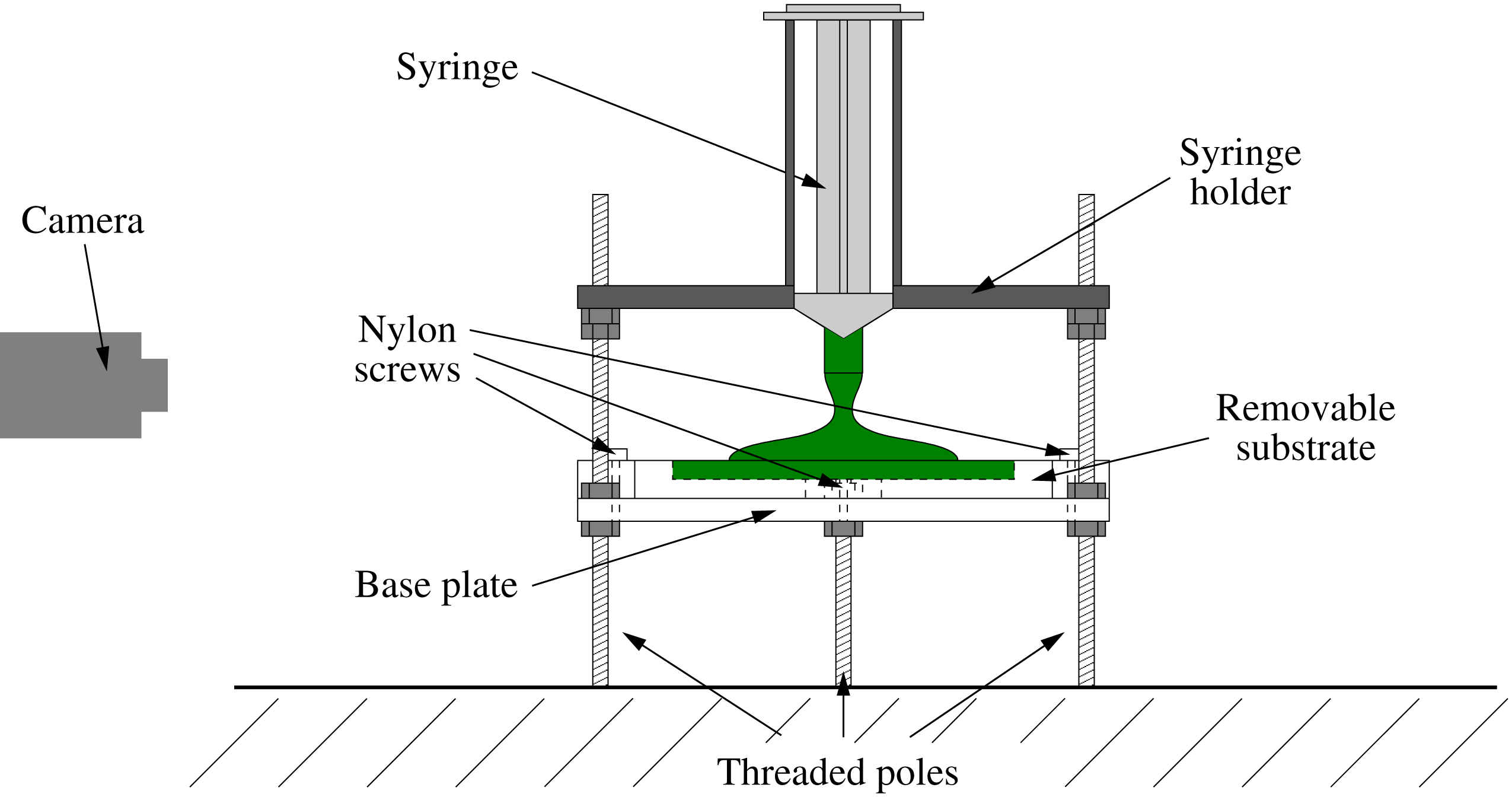
Schematic diagram of the experimental apparatus.

A schematic diagram of the experimental apparatus used to examine the spreading following deposition of a drop on a substrate is shown in figure 1. The substrate (a Perspex plate of dimensions
 $100\times 100\times 10~\text{mm}$
with surfaces milled to an accuracy of
 $\pm 0.02~\text{mm}$
) was secured to the base plate with three finger-tight nylon screws. A featureless, flat substrate was used for the dry spreading experiments, whereas for spreading on a viscous layer, centred, circular troughs with a diameter of 60.5 mm and depths of
 $0.52\pm 0.02~\text{mm}$
,
 $0.85\pm 0.03~\text{mm}$
,
 $1.51\pm 0.04~\text{mm}$
and
 $1.95\pm 0.03~\text{mm}$
were milled into the plate into which a uniform film of liquid was deposited prior to experimentation. The substrate was supported on a Perspex base plate, which was adjustably mounted on three vertical, threaded poles (with a pitch of 1.25 mm) using nuts, thus allowing accurate levelling to
 $\pm 0.1^{\circ }$
. The fluid was deposited using a standard 10 ml plastic syringe whose inner diameter was enlarged to
 $8\pm 0.05~\text{mm}$
to facilitate the manual deposition of the highly viscous liquid. To ensure reproducible deposition of the fluid, we placed the syringe inside a tightly fitting removable holder which was mounted on the three vertical, threaded poles, allowing its level to be adjusted in a similar way to the base plate. The accurate levelling of both base plate and syringe holder was essential to ensure axisymmetric spreading. Side view images of the backlit drop were captured with a wall-mounted CCD camera (Pulnix TM-6740CL,
 $640\times 480~\text{pixel}$
).
We performed the spreading experiments with glucose syrup (Cerestar UK Ltd.), which is a transparent, highly viscous Newtonian liquid. In order to enhance contrast in the images, the glucose syrup was dyed using green food colouring. Mixing of the dye entrained air bubbles, which were left to rise out of the fluid overnight. The experiments were performed by filling the syringe with 5 ml of glucose syrup and wiping any excess fluid from the outside of the nozzle with a dry paper towel. The filled syringe was then placed inside the syringe holder, the image acquisition was initiated, and the plunger of the syringe was displaced manually to empty the syringe barrel within a deposition time of
 $2.5\pm 0.5~\text{s}$
.
We measured the density of the glucose syrup at the laboratory temperature of
 $20.5\pm 0.5\,^{\circ }\text{C}$
to be
 $\unicode[STIX]{x1D70C}=1387\pm 1~\text{kg}~\text{m}^{-3}$
by accurately weighing five samples of known volume between 5 and 20 ml. We determined the viscosity of glucose syrup at the laboratory temperature, using a Brookfield R/S-Plus (SST) rheometer with a concentric cylinder CC25 geometry. We performed shear rate measurements with linear increase from zero to a maximum value of
 $25~\text{s}^{-1}$
with increments of
 $1~\text{s}^{-1}$
, applying a cycle of incremental shear rate increase and decrease. The total experimentation time was 50 s, with one measurement taken every second. Hence, we recorded 50 viscosity measurements and these experiments confirmed that the viscosity of glucose syrup is independent of the shear rate within the investigated parameter range. The resulting averaged dynamic viscosity is
 $\unicode[STIX]{x1D707}=119.73\pm 0.86~\text{Pa}~\text{s}$
. The surface tension of the glucose syrup was taken from the literature (Montañez-Soto et al.
Reference Montañez-Soto, Machuca, González, Nicanor and González-Cruz2013) to be
 $\unicode[STIX]{x1D70E}=55.0\pm 0.6\times 10^{-3}~\text{N}~\text{m}^{-1}$
.
2.1.2 Substrate preparation
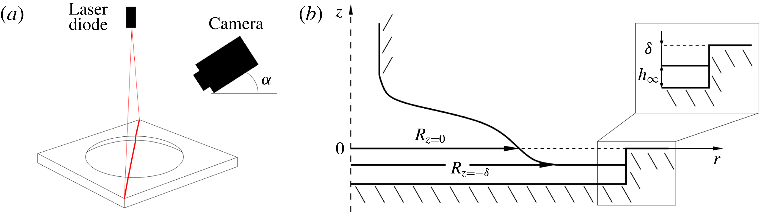
Schematic diagrams of (a) the method to determine the layer thickness and (b) the underfilled trough, illustrating the thickness of the layer
 $h_{\infty }$
and the distance to the upper surface of the substrate
 $\unicode[STIX]{x1D6FF}$
. Also specified in the schematic are the radius as observed by the camera,
 $R_{z=0}$
, and the actual radius of the spreading front,
 $R_{z=-\unicode[STIX]{x1D6FF}}$
.

When performing the experiments in which the drop is deposited on a uniform layer of the same fluid, we prepared the substrate by slightly overfilling the trough and then scraping off the excess fluid with a square-edged ruler. The ruler was moved at an angle of around
 $30^{\circ }$
and with low speed to avoid the washboard instability (Hewitt, Balmforth & McElwaine Reference Hewitt, Balmforth and Mcelwaine2012) at the free surface. This method had the advantage of rapid deposition, thus preventing the formation of a skin due to evaporation and subsequent crystallisation at the surface (Edwards Reference Edwards2000; Lees Reference Lees2012). Since a certain amount of the (highly viscous) fluid adhered to the scraper this procedure resulted in an underfilled trough, with the surface of the fluid layer located at a distance
 $\unicode[STIX]{x1D6FF}$
below the upper surface of the substrate, as illustrated in figure 2(b). The fact that the initial free surface was located below the upper surface of the substrate meant that part of the free surface was obscured so that the outermost radius of the propagating air–liquid interface that was observable by the wall-mounted CCD camera during spreading,
 $R_{z=0}(t)$
, was smaller than the actual radius of the spreading front,
 $R_{z=-\unicode[STIX]{x1D6FF}}(t)$
. We will return to this issue in § 4.1.
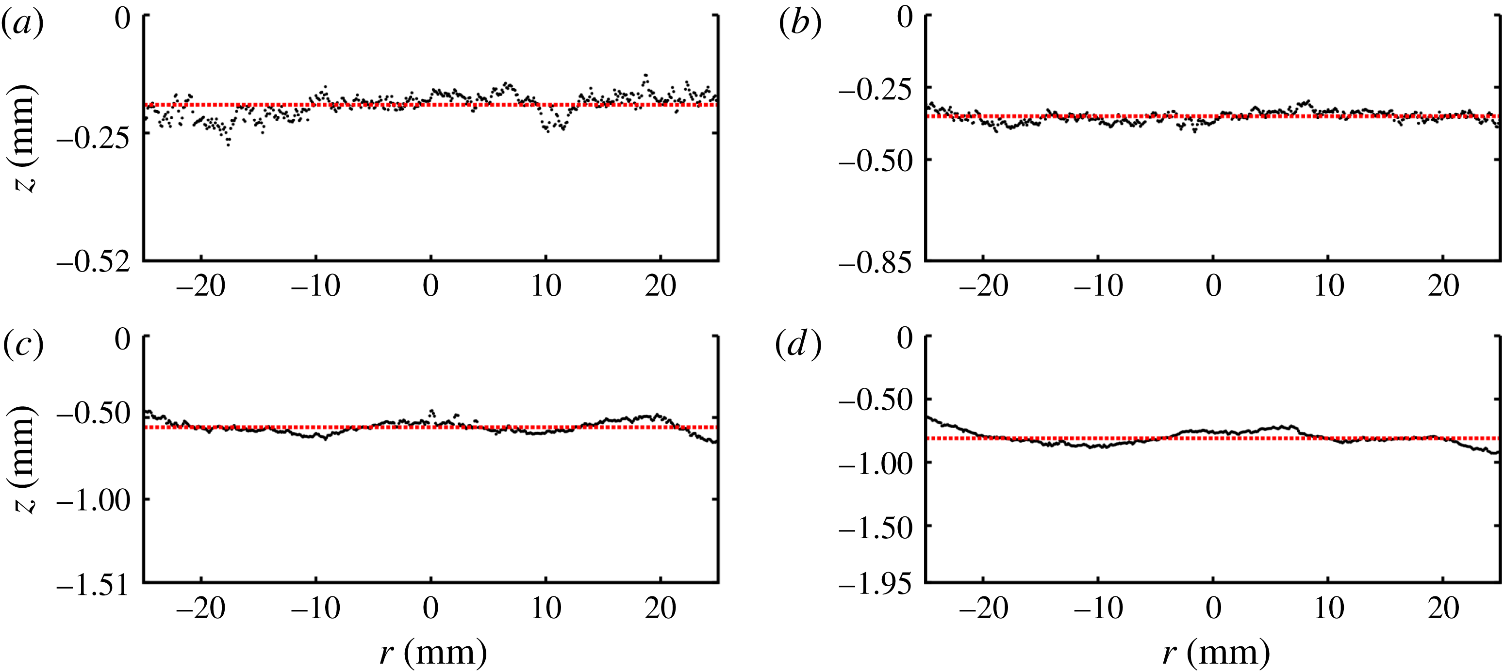
The averaged layer profiles for troughs of depth (a) 0.52 mm, (b) 0.85 mm, (c) 1.51 mm and (d) 1.95 mm. The dashed lines illustrate the approximated uniform layer thicknesses.

We determined
 $\unicode[STIX]{x1D6FF}$
by shining a red laser sheet vertically onto the fluid-filled trough, which was aligned such that the laser captured the entire trough diameter as shown schematically in figure 2(a). We then recorded a still image with a SLR camera (Nikon D7100,
 $6000\times 4000~\text{pixel}$
) which was placed 10 cm above the trough and inclined at
 $\unicode[STIX]{x1D6FC}=16.4\pm 0.1^{\circ }$
from the horizontal. These images were analysed by detecting the position of the laser line relative to the edge of the trough. Sub-pixel resolution was achieved by first isolating the laser line in the images and then fitting a Gaussian profile to the intensity of the red channel of each pixel column across the line in order to find the point of maximum intensity. The averaged layer profiles across four to five measurements are shown in figure 3, where we omitted the error bars of typically 3 %. Omitting the meniscus at the trough edge, we determined the spatially averaged layer thickness in the trough by fitting a straight line to the averaged profiles within the radius
 $r\leqslant 25~\text{mm}$
. We then calculated the standard deviation of the individual profiles from this uniform thickness (illustrated by dashed lines in figure 3). The resulting layer thicknesses are
 $h_{\infty }=0.33\pm 0.06~\text{mm}$
,
 $0.5\pm 0.07~\text{mm}$
,
 $0.95\pm 0.12~\text{mm}$
and
 $1.14\pm 0.13~\text{mm}$
for trough depths of 0.52 mm, 0.85 mm, 1.51 and 1.95 mm, respectively.
2.1.3 Image analysis
We analysed the images that were acquired by the CCD camera using the OpenCV software (Bradski & Kaehler Reference Bradski and Kaehler2008) within a python environment. In order to convert the results from the image analysis into dimensional quantities, a calibration image of a cylindrical object of known dimensions was recorded prior to each experiment, which yielded a spatial resolution of
 $0.111\pm 0.006~\text{mm}~\text{pixel}^{-1}$
. Unavoidable small misalignment of the camera was corrected for in post-processing by rotating the image prior to the analysis, so that the platform edge was perfectly parallel to the image edge. We recorded the spreading of the drop as a sequence of images, taken at a rate of 20 f.p.s. and then analysed the resulting images over a period of up to 100 s from the end of the initial drop deposition. In each image we determined the positions of the air–liquid interface, the upper edge of the substrate and the end of the nozzle, using standard edge detection routines. We implemented these routines, which identify edges based on discontinuities in the intensity profile of the image, in the OpenCV framework. Sub-pixel accuracy was again achieved by exploiting the smooth variations in the intensity profile. We determined the position of the edge based on functional fits to the intensity profile. In particular, we used tanh functions for solid edges (Nalwa & Binford Reference Nalwa and Binford1986), such as the substrate and nozzle edges, and spline functions for the air–liquid interface (Poggio, Torre & Koch Reference Poggio, Torre and Koch1985; Poggio, Voorhees & Yuille Reference Poggio, Voorhees and Yuille1988). The spline fit proved necessary because the interface became increasingly diffuse as the drop spread due to surface reflections. The robustness of the analysis was improved by using the interface position detected in the previous frame of the sequence as an initial condition. Hence, for all images following the initial frame we applied the edge finding routine to a region of
 $\pm 5$
pixels horizontally and
 $\pm 2$
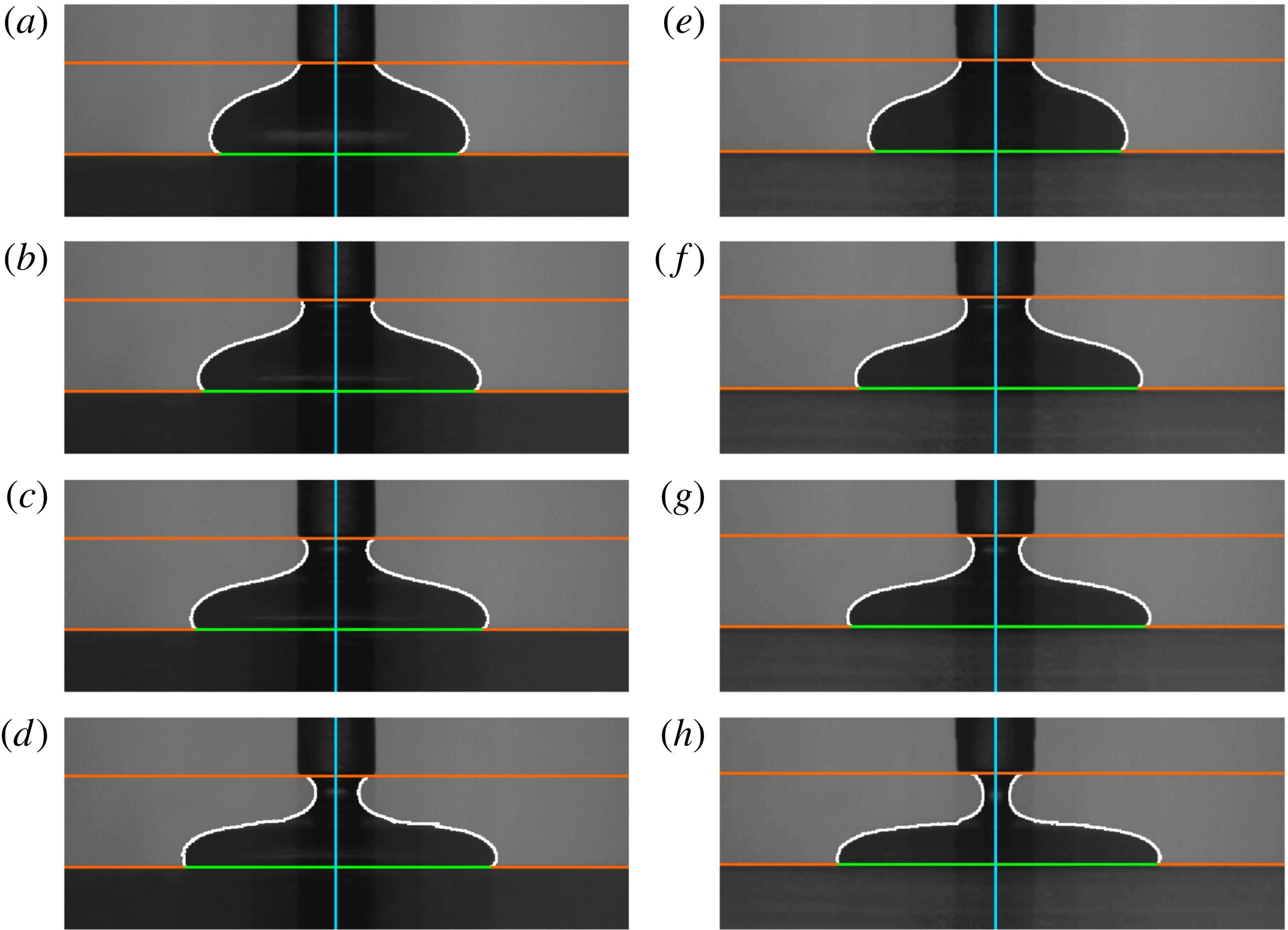
pixels vertically of the interface position located in the preceding frame. We determined the coordinates of the air–liquid interface separately for the left and right sides of each image. The radii obtained from the two sides typically differed by less than 2 %, indicating that the drops tended to spread axisymmetrically. Representative results obtained from our edge detection algorithms are shown in figure 4 where the orange lines indicate the lower end of the nozzle and the platform edge, respectively, the green line the drop diameter at the upper boundary of the substrate and the red line the air–liquid interface. The blue line shows the nozzle centreline. The coordinates of the interface were measured relative to an
 $(r,z)$
-coordinate system that was centred at the intersection of the blue and green lines.
2.2 Experimental results
Side view images of glucose syrup spreading on a dry substrate (a–d) and on a layer of the same fluid of thickness
 $h_{\infty }=0.33~\text{mm}$
(e–h) at different times for a single experiment: (a,e)
 $t=0.0~\text{s}$
, (b,f)
 $t=5.0~\text{s}$
, (c,g)
 $t=10.0~\text{s}$
, (d,h)
 $t=20.0~\text{s}$
. We show the processed images, highlighting the platform edge and nozzle end, centre line, bottom diameter and air–liquid interface.

Sequences of images showing the spreading of a drop of glucose syrup on a dry substrate and on a layer of the same fluid of thickness
 $h_{\infty }=0.33~\text{mm}$
are shown in figure 4. Figure 4(a,e) shows the initial drop configuration immediately after all the fluid has been ejected from the syringe. Figure 4(b–d,f–h) illustrates the subsequent, approximately axisymmetric spreading of the drop. In both cases the spreading rate decreases as the drop spreads out (note the non-uniform time increments between the panels). The radius of the thread of fluid that connects the drop to the nozzle decreases rapidly and the thread ultimately pinches off (not shown here). The detached lower half of the thread then collapses onto the surface of the drop where it tended to create additional reflections which made the subsequent image processing difficult. However, the pinch off of the thread had little effect on the overall spreading dynamics; see computational results in figure 6 below.
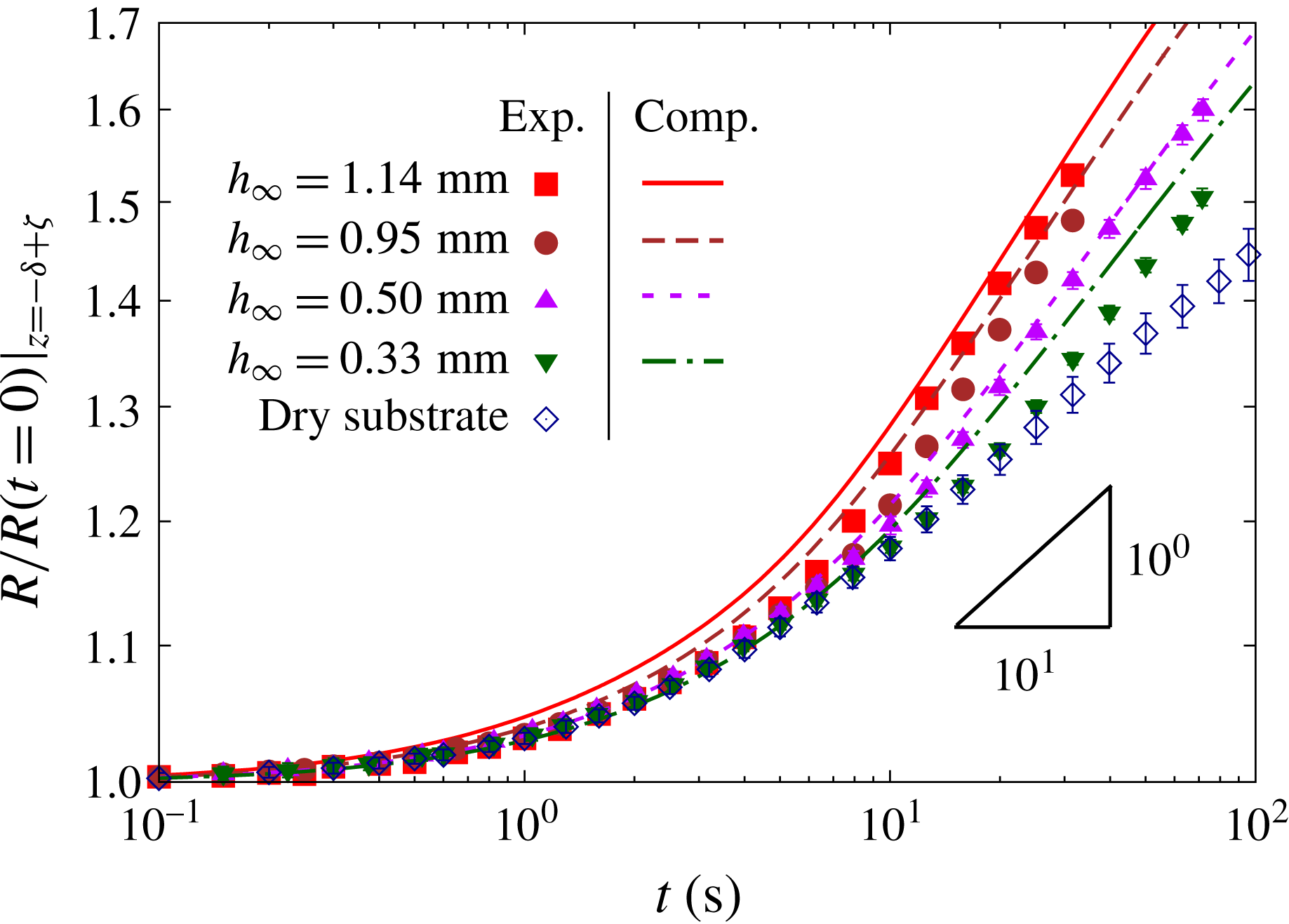
Temporal evolution of the normalised radius,
 $R(t)/R(t=0)|_{z=-\unicode[STIX]{x1D6FF}+\unicode[STIX]{x1D701}}$
, for spreading on layers of fluid of thicknesses
 $h_{\infty }=0.33$
, 0.5, 0.95 and 1.14 mm and on a dry substrate, on a log–log scale. The height at which the radius is measured (
 $\unicode[STIX]{x1D701}=0.81~\text{mm}$
) is illustrated in figure 7 below. Solid lines show the corresponding results of matching computations. Solid and hollow symbols with error bars indicate experimental results for spreading on a fluid layer and on a dry substrate, respectively. The lines show the corresponding numerical results for spreading on a fluid layer.

Figure 5 shows the time evolution of the normalised drop radius
 $R(t)/R(t=0)$
for the spreading on layers of thicknesses
 $h_{\infty }=0.33$
, 0.5, 0.95 and 1.14 mm (solid symbols with error bars) on a log–log scale and contrasts it with the evolution for spreading of an equivalent drop on a dry substrate (hollow symbols with error bars); the lines show the corresponding numerical results for spreading on a fluid layer and will be discussed in § 4.1 below. In order to make the radius evolution comparable across the different configurations we monitored the radius at a vertical distance
 $\unicode[STIX]{x1D701}=0.81~\text{mm}$
above the surface of the undisturbed fluid layer or the dry substrate, respectively (see figure 7). This value of
 $\unicode[STIX]{x1D701}$
was chosen so that for the thickest layer (and hence the largest gap size
 $\unicode[STIX]{x1D6FF}$
), the radius was monitored at the upper edge of the trough,
 $z=0$
.
To within experimental accuracy, the initial evolution of the radii in figure 5 up to a time of approximately 0.5 s is very similar for spreading on a layer of fluid and on a solid substrate. Beyond this time the drop deposited on the dry substrate spreads significantly more slowly than that deposited on the fluid layers. The figure shows that the drop spreading on a dry substrate ultimately follows the power-law behaviour
 $R\propto t^{1/10}$
, which may seem surprising since it matches the power-law behaviour predicted by Tanner’s (Reference Tanner1979) analysis for ‘small’ drops – recall that drops considered here are ‘large’. However, the behaviour is, in fact, consistent with observations by Cazabat & Cohen-Stuart (Reference Cazabat and Cohen-Stuart1986) who performed detailed experiments of the spreading of ‘large’ silicone oil drops on a smooth glass surface. Their experiments show that there is an intermediate regime during which the evolution of the drop radius follows an
 $R\propto t^{1/10}$
power law. Eventually a transition occurs to spreading that follows the
 $R\propto t^{1/8}$
power law that is expected from scaling arguments based on a balance between gravitational and viscous forces (Lopez et al.
Reference Lopez, Miller and Ruckenstein1976; Huppert Reference Huppert1982). The time at which the transition between the two regimes occurs increases with the fluid viscosity and decreases with the drop size. For the largest drop volume,
 $V=37.9~\unicode[STIX]{x03BC}\text{l}$
, and highest viscosity,
 $\unicode[STIX]{x1D707}=1~\text{Pa}~\text{s}$
, used in their experiments, Cazabat & Cohen-Stuart (Reference Cazabat and Cohen-Stuart1986) report a transition time of
 ${\approx}100~\text{s}$
. Our drops are one order of magnitude larger, but also two orders of magnitude more viscous; we therefore expect this transition to occur beyond the duration of our experiments which were terminated before the drop had spread to the outer edge of the trough.
Over the duration of our experiments the drops spreading on a layer of fluid also approach a power-law behaviour,
 $R\propto t^{n}$
, but with a larger exponent,
 $n>1/10$
, which increases with the layer thickness
 $h_{\infty }$
, indicating faster spreading on thicker layers.
3 Theory and computations
In order to systematically study the influence of the layer thickness on the spreading of a viscous drop on a layer of the same fluid we developed a theoretical/computational model of the spreading process. This enabled us to extend the observation times beyond those accessible experimentally and allowed the detailed visualisation of the flow in the layer, particularly in the vicinity of the advancing front.
3.1 The model
We model the glucose syrup as an incompressible Newtonian fluid and assume the flow to be axisymmetric. We non-dimensionalise the governing equations by choosing the cube root of the drop volume,
 $V^{1/3}$
, as the length scale,
 ${\mathcal{L}}$
, and, assuming that the flow is governed by a balance between viscous and gravitational forces, scale the velocities on
 ${\mathcal{U}}=\unicode[STIX]{x1D70C}g{\mathcal{L}}^{2}/\unicode[STIX]{x1D707}$
. We non-dimensionalise the pressure on the associated scale,
 $\unicode[STIX]{x1D707}{\mathcal{U}}/{\mathcal{L}}=\unicode[STIX]{x1D70C}g{\mathcal{L}}$
, and time on the intrinsic time scale
 ${\mathcal{L}}/{\mathcal{U}}$
. The flow is then governed by the non-dimensional Navier–Stokes equations
 $$\begin{eqnarray}Re\left(\frac{\unicode[STIX]{x2202}\boldsymbol{u}}{\unicode[STIX]{x2202}t}+(\boldsymbol{u}\boldsymbol{\cdot }\unicode[STIX]{x1D735})\boldsymbol{u}\right)=-\unicode[STIX]{x1D735}p-\boldsymbol{e}_{z}+\unicode[STIX]{x1D6FB}^{2}\boldsymbol{u},\quad \text{and}\quad \unicode[STIX]{x1D735}\boldsymbol{\cdot }\boldsymbol{u}=0,\end{eqnarray}$$
where the Reynolds number,
 $Re=\unicode[STIX]{x1D70C}{\mathcal{U}}{\mathcal{L}}/\unicode[STIX]{x1D707}$
, the ratio of inertial to viscous forces, is equivalent to the Archimedes number,
 $Re=Ar=\unicode[STIX]{x1D70C}^{2}g{\mathcal{L}}^{3}/\unicode[STIX]{x1D707}^{2}$
.
Because the glucose syrup is highly viscous the drop takes a while to disconnect from the syringe nozzle and during this time it already spreads significantly. We therefore included the nozzle into the computational model. The fluid is subject to the no-slip boundary condition
 $\boldsymbol{u}=\mathbf{0}$
on the inner boundary of the nozzle and on the surface of the substrate, including the outer edge of the trough where we assume the contact line to be pinned. We denote the position vector to the free surface by
 $\boldsymbol{R}_{fs}(s,t)$
, where
 $s$
is the arclength along the air–liquid interface, at which we apply the dynamic and kinematic boundary conditions,
 $$\begin{eqnarray}\unicode[STIX]{x1D748}\boldsymbol{\cdot }\boldsymbol{n}=\frac{1}{Bo}\unicode[STIX]{x1D705}\boldsymbol{n}-p_{ext}\boldsymbol{n},\end{eqnarray}$$
and
 $$\begin{eqnarray}\left(\boldsymbol{u}-\frac{\unicode[STIX]{x2202}\boldsymbol{R}_{fs}}{\unicode[STIX]{x2202}t}\right)\boldsymbol{\cdot }\boldsymbol{n}=0.\end{eqnarray}$$
Here
 $\unicode[STIX]{x1D748}$
is the fluid stress tensor,
 $\unicode[STIX]{x1D705}$
is twice the mean curvature of the air–liquid interface (negative for a spherical drop) and
 $\boldsymbol{n}$
its outer unit normal (pointing out of the liquid).
 $p_{ext}$
is the external (atmospheric) pressure that we subsequently set to zero. The Bond number,
 $Bo=\unicode[STIX]{x1D70C}g{\mathcal{L}}^{2}/\unicode[STIX]{x1D70E}$
, the ratio of gravitational to surface-tension forces, plays the role of the capillary number,
 $Bo=Ca=\unicode[STIX]{x1D707}{\mathcal{U}}/\unicode[STIX]{x1D70E}$
.
3.2 Parameter regime
Using the physical parameter values from our experiments (see § 2.1.1) yields the characteristic length, velocity and time scales,
 ${\mathcal{L}}=V^{1/3}=17.1\times 10^{-3}~\text{m}$
,
 ${\mathcal{U}}=\unicode[STIX]{x1D70C}g{\mathcal{L}}^{2}/\unicode[STIX]{x1D707}=33.2\times 10^{-3}~\text{m}~\text{s}^{-1}$
and
 ${\mathcal{T}}={\mathcal{L}}/{\mathcal{U}}=0.52~\text{s}$
, respectively. This yields a Reynolds/Archimedes number of
 $Re=Ar=6.58\times 10^{-3}$
and a Bond/capillary number of
 $Bo=Ca=72.34$
, indicating that, as assumed, the overall motion of the drop is likely to be quasi-steady and dominated by a balance between gravitational and viscous forces. Capillary forces are likely to have little effect on the overall motion because the capillary length
 $L_{c}=(\unicode[STIX]{x1D70E}/(\unicode[STIX]{x1D70C}g))^{1/2}=2\times 10^{-3}~\text{m}$
is much smaller than the size of the drop,
 ${\mathcal{L}}\gg L_{c}$
. Therefore, we classify the drops used in our experiments as ‘large’. However, surface tension can (and, as we will show below, does) still have a localised effect on the flow in regions where the interface curvature is larger than
 $1/L_{c}$
.
3.3 Numerical solution
We used our open-source library oomph-lib (Heil & Hazel Reference Heil, Hazel, Schäfer and Bungartz2006) to discretise the arbitrary Lagrangian–Eulerian (ALE) form (Donea, Giuliani & Halleux Reference Donea, Giuliani and Halleux1982) of the governing equations in an axisymmetric
 $(r,z)$
-coordinate system by finite elements, using LBB-stable (Sani & Gresho Reference Sani and Gresho2000) six-noded, triangular Taylor–Hood (
 $P_{2}P_{1}$
) elements (Taylor & Hood Reference Taylor and Hood1973) on an unstructured moving mesh. Time derivatives were discretised using the second-order accurate backward differentiation formula (BDF2) (Sani & Gresho Reference Sani and Gresho2000). The initial mesh was generated by Triangle (Shewchuk Reference Shewchuk, Lin and Manocha1996), using the shape of the air–liquid interface extracted from the experiments. We re-constructed the obscured part of the free surface (see discussion in § 2.1.2) by connecting the visible part of the air–liquid interface to the undisturbed, uniform fluid layer ahead of the drop using a spline fit. The simulation was started from rest,
 $\boldsymbol{u}(t=0)=\mathbf{0}$
. We note that in the experiments, the fluid is not at rest following deposition. In order to assess the effect of our idealised initial condition, we repeated selected computations, starting with the drop shape observed 1 s after the end of the deposition. The results are qualitatively unchanged, confirming that the system’s evolution is quasi-steady. Quantitative differences arise due to slight differences between the observed and computed shapes; see figure 7. However, the long-term evolution of the drop remained unaffected. The mesh deformation in response to the displacement of the air–liquid interface was determined by solving the equations of large-displacement elasticity, treating the fluid mesh as a pseudo-solid body. To avoid overly large distortion of the elements we re-generated the mesh at regular intervals and transferred the solution between the meshes by projection. When re-generating the mesh, we biased the element sizes by spatial error estimates obtained from the Z2 flux-recovery error estimator (Zienkiewicz & Zhu Reference Zienkiewicz and Zhu1992), using the entries in the rate-of-strain tensor as the generalised fluxes. This methodology has previously been used and validated in various other applications (e.g. Hewitt et al.
Reference Hewitt, Hazel, Clarke and Denier2011; Hazel et al.
Reference Hazel, Heil, Waters and Oliver2012; Pihler-Puzović et al.
Reference Pihler-Puzović, Juel, Peng, Lister and Heil2015). Simulations were typically performed with a (dimensional) time step of 0.075 s and
 $O(800)$
elements. The accuracy of our numerical results was assessed by repeating selected computations with higher spatial and temporal resolution; see figure 8 below.
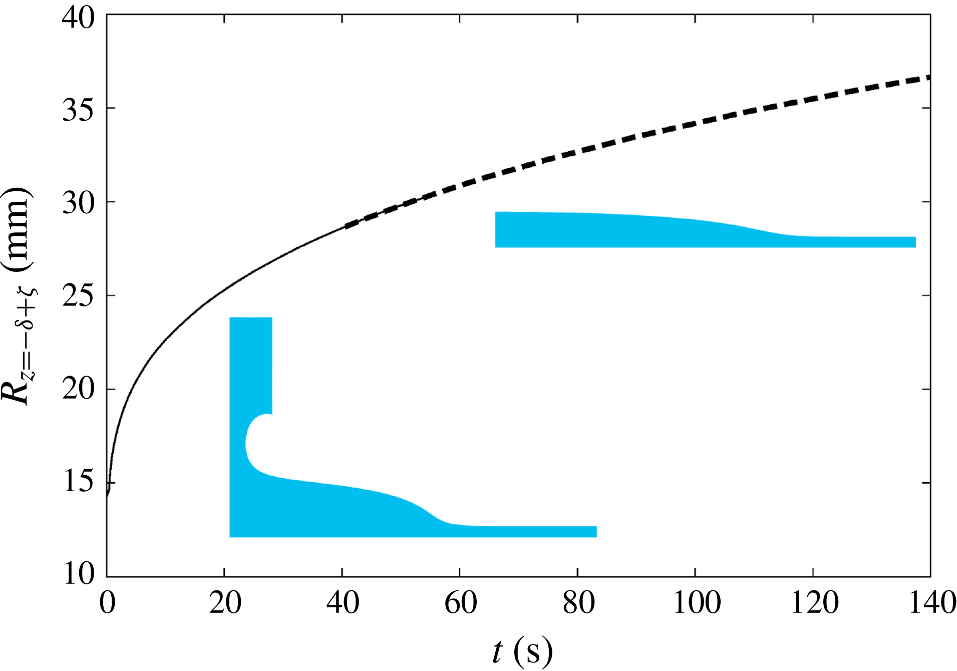
Temporal evolution of the computed drop radius,
 $R(t)|_{z=-\unicode[STIX]{x1D6FF}+\unicode[STIX]{x1D701}}$
, for spreading on a layer of fluid of thickness
 $h_{\infty }=1.14~\text{mm}$
. The height at which the radius is measured, is
 $\unicode[STIX]{x1D701}=0.05~\text{mm}$
. The thick dashed line shows the radius evolution following manual pinch off of the thread at
 $t=40.6~\text{s}$
. The insets show computed characteristic drop shapes before and after pinch off.

In the experiments the liquid thread between the drop and the nozzle eventually pinches off, but, as mentioned above, this appeared to have little effect on the long-term spreading dynamics. In order to enable the direct comparison with experiments we included the nozzle in our simulations but did not attempt to resolve the pinch-off process in detail. Instead, we simply cut the mesh when the radius of the thread dropped below
 $0.5\times 10^{-3}~\text{m}$
and then restarted the simulations. To assess the effect of this manual and somewhat ad hoc intervention we recorded the evolution of the drop radius in two separate simulations, which are shown in figure 6. In one we cut the thread when its minimum radius had dropped below the threshold and restarted the simulation (shown by the thick dashed line in figure 6); in the other we continued the computation without any intervention (shown by the thin solid line in figure 6). The evolution of the drop radii obtained from the two simulations agreed to within graphical accuracy, as indicated by the region of overlap for
 $40\leqslant t\leqslant 60~\text{s}$
– the interval during which pinch off is observed in the experiments. Moreover, the shape of the curve in figure 6 is continuous across the two simulations, confirming that the pinch off has little effect on the overall behaviour.
4 Results
4.1 Comparison between experiments and computations
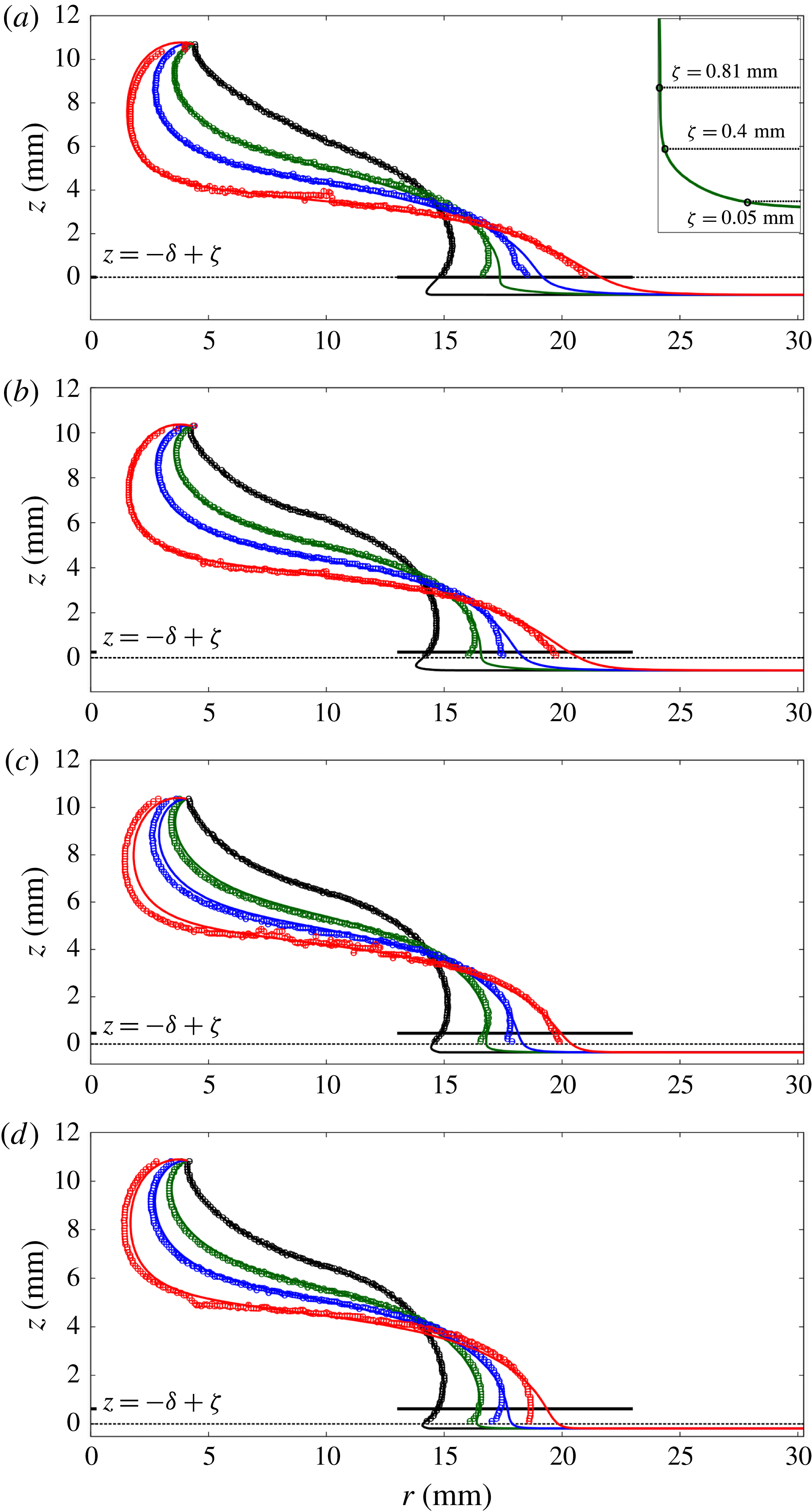
Free surface at times
 $t=0$
(black), 5 (green), 10 (blue) and 20 s (red) for layer thicknesses of (a)
 $h_{\infty }=1.14~\text{mm}$
, (b)
 $h_{\infty }=0.95~\text{mm}$
, (c)
 $h_{\infty }=0.5~\text{mm}$
, and (d)
 $h_{\infty }=0.33~\text{mm}$
, compared against the respective experiments. Lines represent the computational predictions; symbols show the experimental data, with error bars indicating the pixelation error of the image analysis. The thick solid horizontal line illustrates the height
 $z=-\unicode[STIX]{x1D6FF}+\unicode[STIX]{x1D701}$
at which the radius is recorded, while the dotted horizontal line shows the upper edge of the substrate. Below this line the air–liquid interface is obscured in the experiments. The inset in (a) shows the different measurement heights used to obtain the data shown in figure 8.

Figure 7 shows snapshots of the shapes of the spreading drops (solid lines) and compares them against the experimentally observed shapes of the air–liquid interface (symbols with error bars; the latter representing the pixelation error of the image analysis). Overall, there is good quantitative agreement between the computations and experiments, except near the advancing front, where the experiments systematically lag behind the computations. This might be due to the crystallisation and associated property changes of the glucose syrup when in contact with air, as discussed in § 2.1.2. Despite our best efforts in keeping the time scale between the layer preparation and drop deposition as short as possible, the fluid layer may have started to crystallise, resulting in an increased viscosity near the surface and hence slower spreading. One would expect this effect to be more pronounced for thinner layers and this is indeed consistent with our observations in figure 7 where the largest deviation is observed for the thinnest layer. During the initial deposition the drop adopts a shape in which it slightly overhangs the undisturbed fluid layer. This creates a region of high local curvature on the air–liquid interface. Surface-tension forces are significant in this region and lead to a rapid radial expansion of the drop in this region until the free surface adopts a wedge-like shape. The formation of this wedge is delayed with decreasing layer thickness.
We now return to figure 5 to compare the computed temporal evolution of the normalised drop radius
 $R(t)/R(t=0)$
at a vertical distance
 $\unicode[STIX]{x1D701}=0.81~\text{mm}$
above the undisturbed fluid layer with the experimental measurements. (The height at which the radius is measured is indicated by the thick horizontal lines in figure 7.) We note that for all layer thicknesses the experiments are slightly lagging behind the computations with a maximum error of around 5 %. For large times,
 $t>20~\text{s}$
, the experimental and computational data both approach straight lines in the log–log plot; the slopes (and hence the associated power-law exponent,
 $n$
) of the experimental and computational data agree very well.
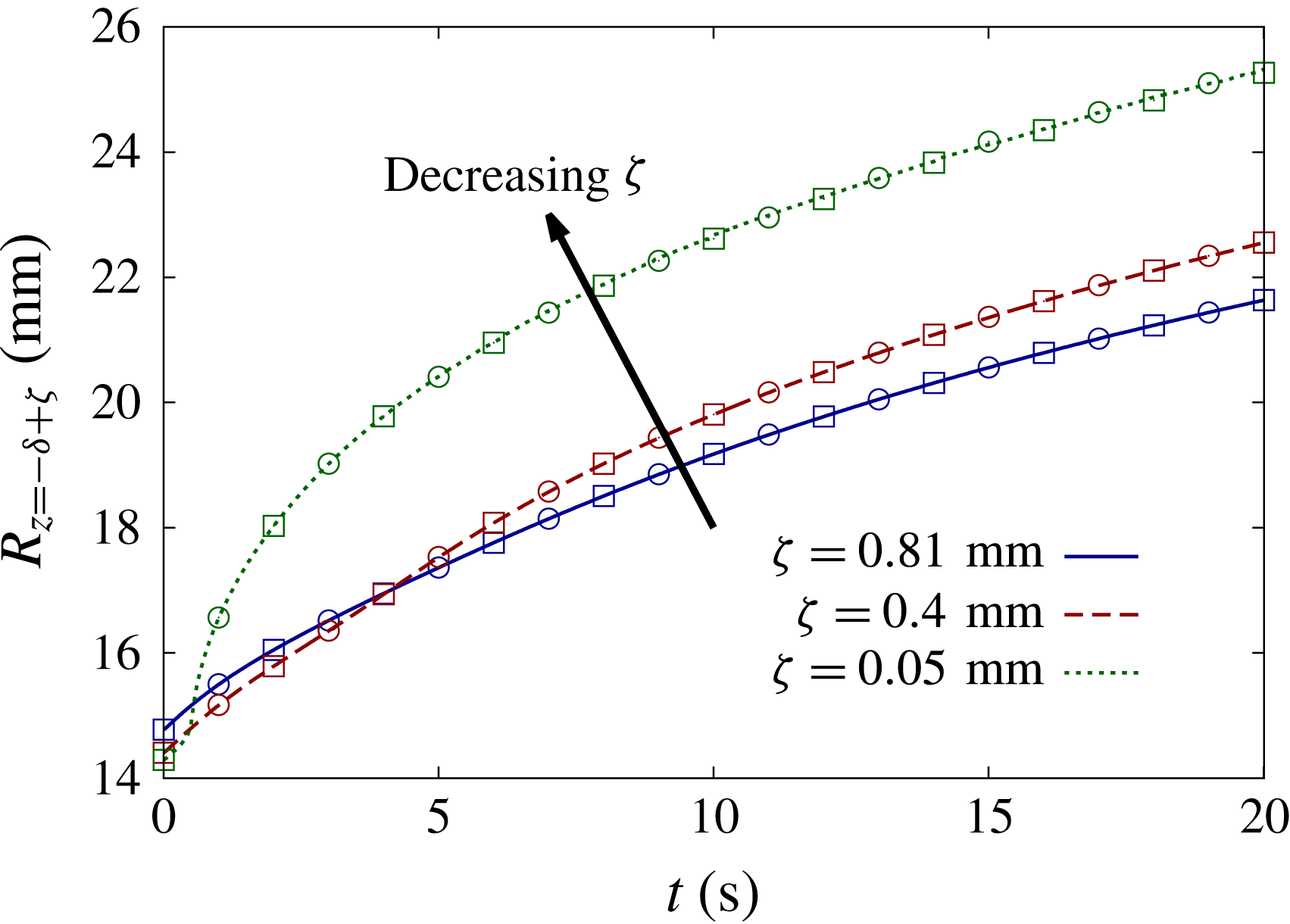
Temporal evolution of the computed drop radius at different measurement heights,
 $\unicode[STIX]{x1D701}$
, for the spreading on a layer of thickness
 $h_{\infty }=1.14~\text{mm}$
(as shown in figure 7
a). The squares (circles) represent data obtained when the computation is performed with twice the spatial (temporal) resolution.

We have already pointed out that we measured the drop radius at a fixed height,
 $\unicode[STIX]{x1D701}=0.81~\text{mm}$
, above the undisturbed fluid layer, because in the experiments with the thickest fluid layer the air–liquid interface is obscured below this level. However, even if this was not the case, there is always some ambiguity about the specific height at which the drop radius is monitored. This is because, unlike the case of spreading on a dry substrate, in our set-up there is no clearly defined contact line which identifies the outer boundary of the drop. It is therefore important to assess how the choice of
 $\unicode[STIX]{x1D701}$
affects the results. For this purpose figure 8 shows the temporal evolution of the drop radius for the thickest layer (
 $h_{\infty }=1.14~\text{mm}$
; the case shown in figure 7
a) at heights of
 $\unicode[STIX]{x1D701}=0.81$
, 0.4 and 0.05 mm above the undisturbed fluid layer; these heights are shown in the inset in figure 7(a). The evolution of the radius at
 $\unicode[STIX]{x1D701}=0.81~\text{mm}$
corresponds to the experimentally observable evolution,
 $R_{z=0}(t)$
. During the early stages of the system’s evolution when the drop overhangs the undisturbed fluid layer the drop radius recorded at
 $\unicode[STIX]{x1D701}=0.81~\text{mm}$
exceeds the radii recorded at smaller heights. Surface tension then acts to smooth out the highly curved region of the air–liquid interface until the advancing front of the drop adopts the characteristic wedge shape shown in figure 7. In this regime the radius increases with a decrease in the height at which it is measured. It appears that once the drop has reached this regime, the slope of the different curves (and hence the associated power-law exponent,
 $n$
) becomes independent of the height at which the radius is measured.
4.2 The flow field and its dependence on the layer thickness at early times
Illustration of the computed flow fields for different layer thicknesses. The colour contours represent the magnitude of the velocity
 $|\boldsymbol{u}|=(u_{r}^{2}+u_{z}^{2})^{1/2}$
, ranging from
 $0~\text{m}~\text{s}^{-1}$
(blue) to
 $0.3\times 10^{-3}~\text{m}~\text{s}^{-1}$
(red) for layer thicknesses of
 $h_{\infty }=0.005$
and 0.5 mm and
 $0.6\times 10^{-3}~\text{m}~\text{s}^{-1}$
for a layer thickness of
 $h_{\infty }=5~\text{mm}$
. The thick solid lines are representative instantaneous streamlines.

Snapshots of the computed free surface during the early stages of the system’s evolution for a layer thickness of
 $h_{\infty }=5~\text{mm}$
. The thick line shows the initial condition at
 $t=0~\text{s}$
; the remaining lines represent the temporal evolution up to
 $t=2~\text{s}$
in increments of 0.5 s, with increasing time indicated by the arrow. The development of a transient ‘bulge’ ahead of the drop is responsible for the jump in the drop radius (measured at a height of
 $\unicode[STIX]{x1D701}=0.05~\text{mm}$
above the undisturbed fluid layer, indicated by the dashed line) in figure 11(c).

Plots illustrating the extent of the region over which the drop introduces a disturbance to the fluid layer ahead of itself, for layer thicknesses of (a)
 $h_{\infty }=0.005~\text{mm}$
, (b)
 $h_{\infty }=0.5~\text{mm}$
and (c)
 $h_{\infty }=5~\text{mm}$
. The black solid lines indicate the drop radius,
 $R(t)$
, while red dashed lines represent the outer radius,
 $R_{disturb}(t)$
, of the region within which the fluid layer is disturbed. Note the different scales of the radius axes.

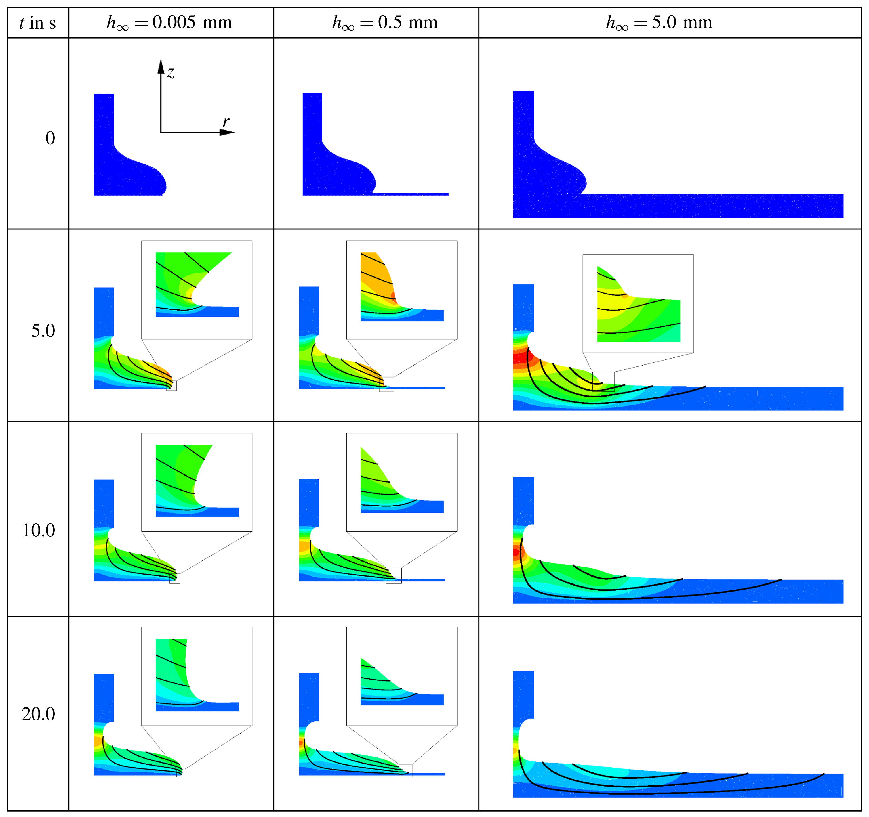
Figure 9 illustrates the flow field and its dependence on the layer thickness which is varied by three orders of magnitude, from
 $h_{\infty }=0.005~\text{mm}$
in the left column to
 $h_{\infty }=5~\text{mm}$
in the right column. These layer thicknesses are representative of three different spreading behaviours, which we refer to as ‘spreading’ (left), ‘wedging’ (middle) and ‘sinking’ (right). The figures show snapshots of the evolving fluid domain (note the non-uniform time increments) and illustrate the flow field by showing representative instantaneous streamlines (thick solid lines); the colour contours indicate the magnitude of the velocity,
 $|\boldsymbol{u}|=(u_{r}^{2}+u_{z}^{2})^{1/2}$
.
For a layer thickness of
 $h_{\infty }=0.005~\text{mm}$
the drop spreads in manner that is very similar to the spreading on a dry substrate (de Gennes Reference de Gennes1985; Bonn et al.
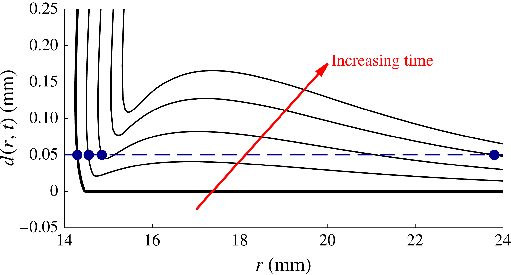
Reference Bonn, Eggers, Indekeu, Meunier and Rolley2009). The fluid layer essentially acts as a passive precursor film and there is minimal flow ahead of the spreading drop. As the layer thickness increases the drop disturbs the fluid layer over a greater distance ahead of itself and the outer edge of the drop ultimately adopts a wedge-like shape – we refer to this behaviour as ‘wedging’. For even thicker films there is significant flow into the layer ahead of the advancing front. The drop now ‘sinks’ rather than ‘spreads’ and the redistribution of fluid into the initially undisturbed fluid layer causes the formation of a transient bulge ahead of the drop. The formation of this bulge is illustrated (for a layer thickness of
 $h_{\infty }=5~\text{mm}$
) in figure 10 where we zoomed into the region near the outer edge of the drop (note the different scales for the radial and vertical axes). The figure also shows that the presence of the bulge leads to an ambiguity in the definition of the drop radius: the dashed line in figure 10 shows the level at which the maximum radius of the air–liquid interface is recorded. As the bulge wells upwards, its free surface intersects the measurement height, causing the drop radius to suddenly jump outwards. For sufficiently large times, the bulge is levelled by gravity and figure 9 shows that the air–liquid interface then adopts a wedge-like shape, but with a much shallower angle than for the intermediate layer thickness of
 $h_{\infty }=0.5~\text{mm}$
.
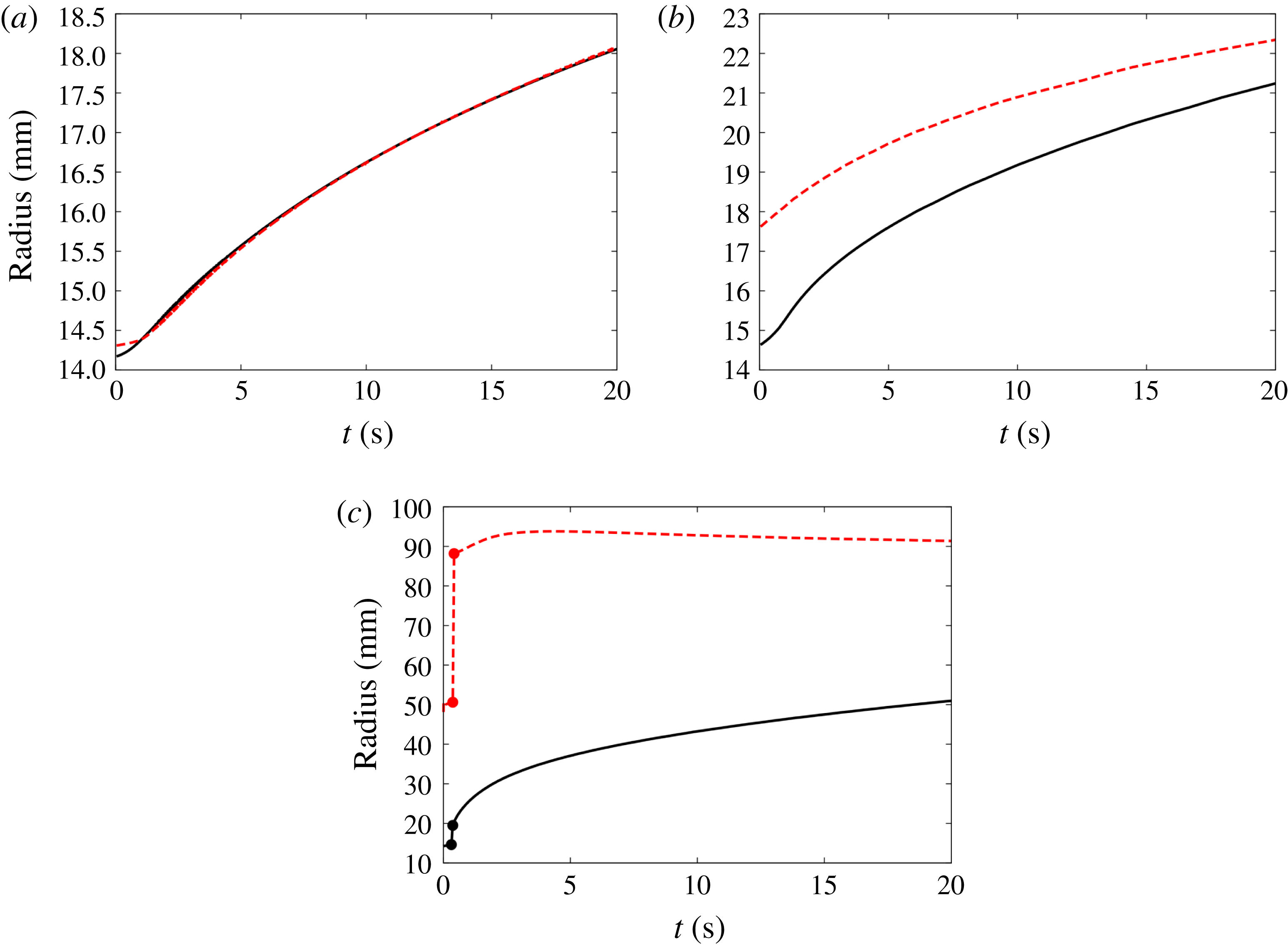
In order to characterise the difference between the three regimes quantitatively we plot in figure 11 the evolution of the drop radius
 $R(t)$
(i.e. maximum radius of the air–liquid interface at a measurement height of
 $\unicode[STIX]{x1D701}=0.05~\text{mm}$
; solid line) and the outer radius
 $R_{disturb}(t)$
of the region within which the spreading drop introduces a noticeable disturbance to the layer (dashed line). For this purpose we defined
 $R_{disturb}(t)$
as the maximum radius at which the magnitude of the fluid velocity at the free surface exceeded a fixed threshold, chosen as
 $2.4\times 10^{-3}~\text{mm}~\text{s}^{-1}$
(which is approximately 1 % of the maximum velocity in the bulk of the drop). The figure shows that for
 $h_{\infty }=0.005~\text{mm}$
, when the drop is in the ‘spreading’ regime (figure 11
a) the perturbation to the layer remains confined to a very small region ahead of the drop; the curves representing
 $R(t)$
and
 $R_{disturb}(t)$
are virtually indistinguishable over most of the period analysed. In the ‘wedging’ regime (figure 11
b) the region within which the fluid layer is disturbed extends as far as 20 % ahead of the drop radius. Both radii increase at a comparable rate and the size of the perturbed region only shrinks very slowly as
 $R(t)$
approaches
 $R_{disturb}(t)$
. Finally, in the ‘sinking’ regime (figure 11
c) the upwelling caused by the rapidly submerging drop creates the bulge whose formation (already illustrated in figure 10) causes a jump in both radii at
 $t\approx 0.3$
s. The drop then spreads slowly into the large disturbed region whose outer radius remains approximately constant.
4.3 Scaling laws at intermediate times
Temporal evolution of the computed normalised excess drop height
 $d_{0}(t)/V^{1/3}$
for (a) the glucose system following pinch off for layer thicknesses of
 $h_{\infty }=0.005$
, 0.01, 0.05, 0.1, 0.33, 0.5, 0.75, 0.95, 1.14, 1.5, 1.75, 2, 2.5, 3.5, 5, 8.5, 12 and 17 mm and (b) the polystyrene system of Cormier et al. (Reference Cormier, McGraw, Salez, Raphaël and Dalnoki-Veress2012) for layer thicknesses of
 $h_{\infty }=0.005$
, 0.01, 0.025, 0.054, 0.1, 0.25, 0.5, 0.75, 0.942, 1.5, 2, 3, 5 and
 $10~\unicode[STIX]{x03BC}\text{m}$
, on a log–log scale. Note that the curves overlap as
 $h_{\infty }\rightarrow 0$
. The insets in (a) show the collapsing thread. The symbols in (b) show selected data of Cormier et al. (Reference Cormier, McGraw, Salez, Raphaël and Dalnoki-Veress2012) with the dashed lines representing the matching computations.

Many theoretical studies of drop spreading on dry substrates or on substrates that are covered with very thin precursor films predict that, at sufficiently large times, the temporal evolution of the drop height and radius follows a power law, with exponents depending on the particular parameter regime considered; see Bonn et al. (Reference Bonn, Eggers, Indekeu, Meunier and Rolley2009).
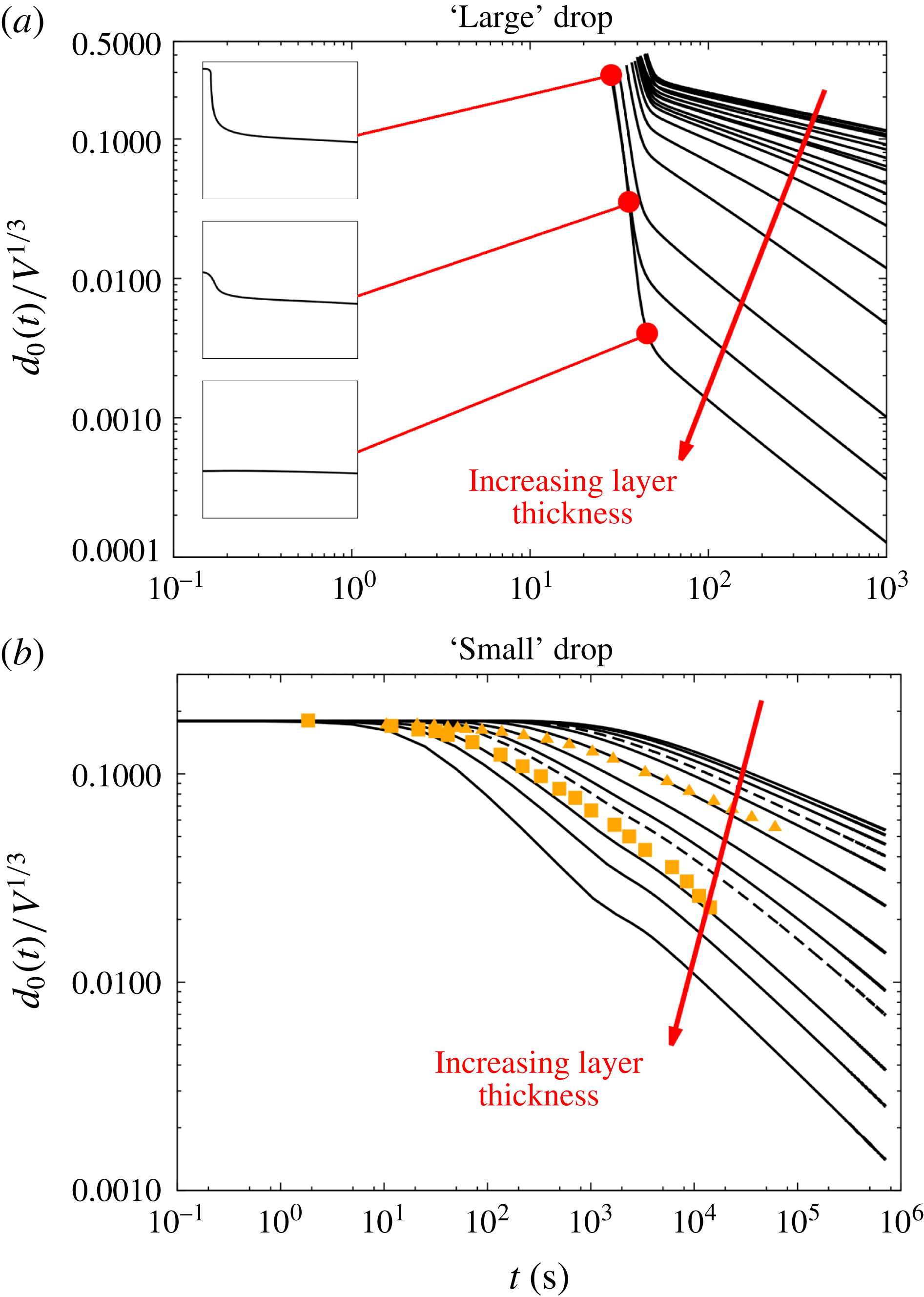
The temporal evolution of the normalised excess drop height,
 $d_{0}(t)=h(r=0,t)-h_{\infty }$
, where
 $h(r,t)$
is the height of the air–liquid interface above the substrate following pinch off, is shown in figure 12(a). The data are shown on a log–log scale for layer thicknesses ranging from
 $h_{\infty }=0.005$
to
 $h_{\infty }=17~\text{mm}$
. Note that here we cover a much wider temporal range than in the experiments which were limited to
 $t<10^{2}~\text{s}$
. For vanishing layer thicknesses,
 $h_{\infty }\rightarrow 0$
, the shape of the curves saturate and overlap (note that due to the very close spacing of the curves for
 $h_{\infty }=0.01$
and
 $h_{\infty }=0.005~\text{mm}$
, they appear as a single thick line in figure 12
a). As the layer thickness increases, the shape of the curves continues to evolve, although the behaviour following pinch off is qualitatively similar in all cases – we observe a rapid decrease in excess height, which represents the collapse of the pinched-off liquid thread into the bulk of the drop (see insets in figure 12
a). This collapse is superimposed on the overall levelling of the drop. Therefore the extent by which the excess drop height decreases in this initial period depends on the layer thickness, with drops on thicker layers levelling more quickly. Following this initial transient regime all curves adopt a power-law behaviour of the form
 $d_{0}(t)\propto t^{-m}$
where the power-law exponent
 $m$
depends on the thickness of the layer. Inspection of the temporal evolution of the drop radius (not shown) shows that it also approaches a power-law behaviour,
 $R(t)\propto t^{n}$
, where
 $m\approx 2n$
. This suggests that the drop evolves in a volume-conserving, self-similar fashion so that its shape at two different times can be obtained by rescaling the vertical and radial coordinates according to the evolution of its excess height and radius, respectively.
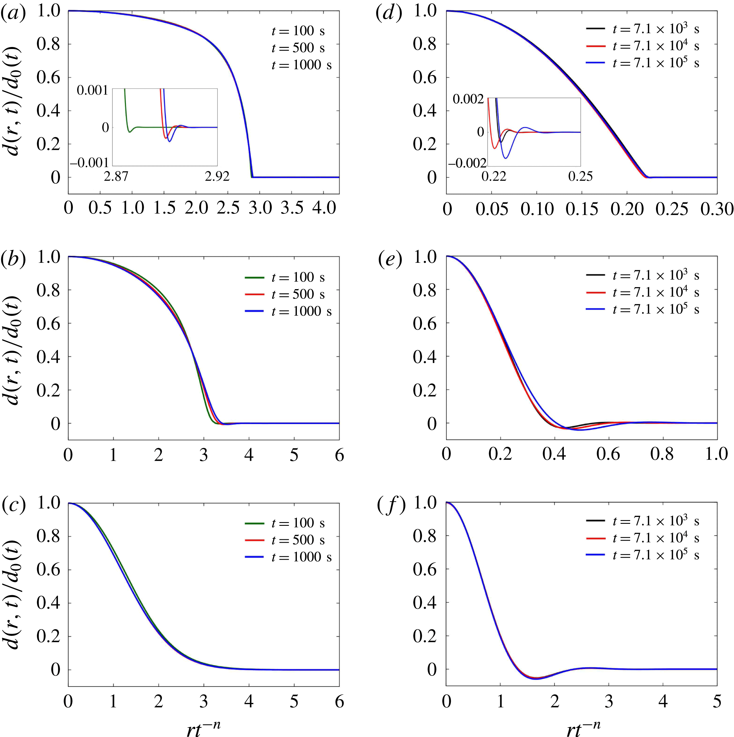
Plots illustrating the self-similarity of the drop shapes for the ‘large’ drop spreading on layers of thicknesses (a)
 $h_{\infty }=0.005~\text{mm}$
, (b)
 $h_{\infty }=0.5~\text{mm}$
, and (c)
 $h_{\infty }=5~\text{mm}$
; and the ‘small’ drop spreading on layers with thicknesses of (d)
 $h_{\infty }=5\times 10^{-3}~\unicode[STIX]{x03BC}\text{m}$
, (e)
 $h_{\infty }=0.5~\unicode[STIX]{x03BC}\text{m}$
, and (f)
 $h_{\infty }=5~\unicode[STIX]{x03BC}\text{m}$
. The insets in (a,d) show the Landau–Levich dimple at the advancing front. The excess drop height
 $d(r,t)=h(r,t)-h_{\infty }$
is normalised on its value at the centre of the drop,
 $d_{0}(t)$
; the radial distances are rescaled on the similarity variable
 $rt^{-n}$
, where the radius and time are non-dimensionalised using the scalings of § 3.1. The power-law exponent
 $n$
, obtained from a fit to the computational data, is (a)
 $n=0.135$
, (b)
 $n=0.1625$
, (c)
 $n=0.469$
, (d)
 $n=0.102$
, (e)
 $n=0.167$
, (f)
 $n=0.246$
.

To assess this, figure 13(a–c) shows overlaid snapshots of the air–liquid interface for drops deposited on layers of thickness (a)
 $h_{\infty }=0.005~\text{mm}$
, (b) 0.5 mm and (c) 5 mm. In each case we show three drop shapes, each taken during the final decade of the evolution shown in figure 12(a) when the excess drop height evolves according to a power law, with a thickness-dependent power-law exponent. To assess the degree to which the drop shapes are self-similar, we scaled the vertical coordinate on the instantaneous excess drop height and rescaled the radial coordinate according the observed power-law behaviour for the radius. The fact that the rescaling leads to a good collapse of the drop shapes onto a master curve confirms that the drop evolves in an approximately self-similar fashion. We note that the rescaling works best for the smallest and largest layer thicknesses shown and will return to this issue in § 4.5. For the thinnest layer the rescaled overall drop shapes are graphically indistinguishable. Only a zoom into the region near the outer edge of the drop (shown in the inset in figure 13
a) shows small deviations in the rescaled drop radius and the position and depth of the characteristic Landau–Levich dimple in the layer thickness just ahead of the drop.
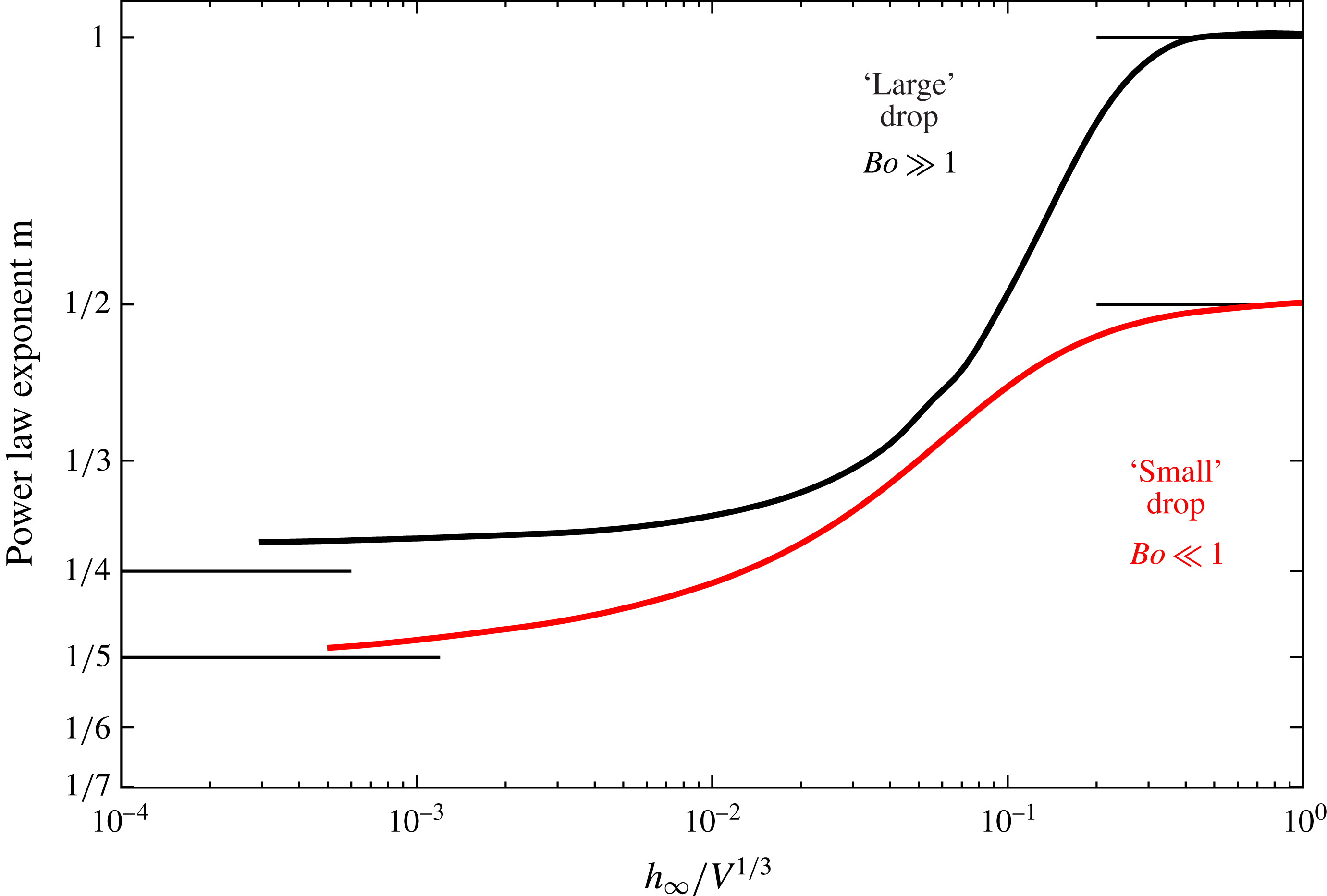
Figure 13(a,d) shows how the power-law exponent
 $m$
for the evolution of the excess drop height (determined by calculating the logarithmic slope of the curves in figure 12
a for
 $t=10^{3}~\text{s}$
) depends on the non-dimensional layer thickness
 $h_{\infty }/V^{1/3}$
. For sufficiently thin fluid layers the power-law exponent approaches a constant value of approximately 0.269 – slightly larger than the value
 $m_{dry}=1/4$
derived by Lopez et al. (Reference Lopez, Miller and Ruckenstein1976) and Huppert (Reference Huppert1982) for gravity-driven spreading on dry substrates. This is consistent with the theoretical results of Kalinin & Starov (Reference Kalinin and Starov1986) and Chebbi (Reference Chebbi1999), who show that the power-law exponents associated with spreading on a thin layer are larger than those associated with spreading on a dry substrate. As the layer thickness increases
 $m$
grows rapidly (indicating faster spreading of drops on thicker layers) before ultimately approaching yet another limit,
 $m\rightarrow 1$
, which we will explain in § 4.5.
4.4 Influence of the drop size
In all the results presented so far the drop volume was set to the value in our experiments. As discussed in § 3.2, our drops are ‘large’ in the sense that their overall size exceeds the capillary length, implying that surface-tension effects only play a minor role in the overall dynamics. We will now consider drops that are ‘small’ (
 $V^{1/3}\ll L_{C}$
or equivalently,
 $Bo\ll 1$
), so that their dynamics is likely to be driven by capillary effects. We choose parameter values to match those of Cormier et al. (Reference Cormier, McGraw, Salez, Raphaël and Dalnoki-Veress2012) who studied the dynamics of a molten polystyrene drop spreading atop a thin layer of the same fluid. In their experiments the drop volume was approximately
 $V=1$
pl – nine orders of magnitude smaller than the drops used in our experiments. Cormier et al. report power-law exponents for the experimentally observed evolution of the excess drop height (
 $m$
in our notation) for layer thicknesses of
 $h_{\infty }=0.942$
and
 $0.054~\unicode[STIX]{x03BC}\text{m}$
, starting from a spherical cap as the initial shape of the drop. Their experimental data points are shown by the symbols in figure 12(b).
Cormier et al. do not specify the material properties of the molten polystyrene used in their experiments. We therefore performed our computations using literature values from other sources. For a temperature of
 $180\,^{\circ }\text{C}$
– the temperature at which the experiments were performed – the density of molten polystyrene is
 $\unicode[STIX]{x1D70C}=976~\text{kg}~\text{m}^{-3}$
(Patnode & Scheiber Reference Patnode and Scheiber1939), the viscosity is
 $\unicode[STIX]{x1D707}=6800~\text{Pa}~\text{s}$
(Fox & Flory (Reference Fox and Flory1948); but see below for a discussion of the effect of variations in this quantity) and the surface tension is
 $\unicode[STIX]{x1D70E}=25.52~\text{mN}~\text{m}^{-1}$
(Kwok et al.
Reference Kwok, Cheung, Park and Neumann1998). Using these values and the much smaller drop volume of
 $V=1$
pl we obtain a Bond number of
 $Bo=Ca=3.78\times 10^{-5}$
and a Reynolds/Archimedes number of
 $Re=Ar=2\times 10^{-16}$
, indicating that we are now in a surface-tension-driven regime.
We performed computations for these parameter values and for layer thicknesses between
 $h_{\infty }=5\times 10^{-3}~\unicode[STIX]{x03BC}\text{m}$
and
 $50~\unicode[STIX]{x03BC}\text{m}$
. The resulting temporal evolution of the excess drop height is shown in figure 12(b). Given the uncertainties about the material properties, there is reasonable agreement with the data from Cormier et al.’s (Reference Cormier, McGraw, Salez, Raphaël and Dalnoki-Veress2012) experiments. The main difference to the data for the ‘large’ drop is (i) the absence of the rapid initial decrease in excess drop height associated with the collapse of the pinched-off thread that detaches from the nozzle which not present here, and (ii) the much longer time scale over which the drop spreads. For sufficiently large times the evolution of the excess drop height again displays a clear power-law behaviour with a thickness-dependent power-law exponent
 $m$
. Figure 13(d–f) shows that the drop shape again evolves in an approximately self-similar fashion over a time interval spanning two orders of magnitude. The lower curve in figure 14 shows the power-law exponent
 $m$
for the long-term evolution of the excess drop height. The overall behaviour is qualitatively similar to that for ‘large’ drops in the sense that an increase in layer thickness again increases the power-law exponent, indicating (relatively) faster spreading. The power-law exponent for the ‘small’ drop is less than that for the ‘large’ drops considered in our own experiments. This reduction is consistent with the trend observed for spreading on dry substrates for which Tanner (Reference Tanner1979) predicts a power-law exponent of
 $m_{dry}=1/5$
for capillary-driven spreading of ‘small’ drops, compared to Lopez et al.’s (Reference Lopez, Miller and Ruckenstein1976) and Huppert’s (Reference Huppert1982) prediction of
 $m_{dry}=1/4$
for the gravity-driven spreading of ‘large’ drops.
Power-law exponent
 $m$
on a log–log scale for the computed excess drop height (
 $d_{0}(t)\propto t^{-m}$
), as function of the non-dimensional layer thickness
 $h_{\infty }/V^{1/3}$
. The data for ‘large’ drops were computed at
 $t=10^{3}~\text{s}$
using parameter values from our experiments; the data for ‘small’ drops are for parameter values for Cormier et al.’s (Reference Cormier, McGraw, Salez, Raphaël and Dalnoki-Veress2012) experiments with drops of molten polystyrene, computed at
 $t=10^{5}~\text{s}$
. The short horizontal lines at
 $h_{\infty }/V^{1/3}\rightarrow 0$
indicate the corresponding power-law exponents predicted by Lopez et al. (Reference Lopez, Miller and Ruckenstein1976) and Tanner (Reference Tanner1979) for spreading of ‘small’ and Huppert (Reference Huppert1982) for spreading of ‘large’ drops, respectively, on dry substrates. The short horizontal lines at
 $h_{\infty }/V^{1/3}=O(1)$
indicate the corresponding power-law exponents in the thick-film limit; see Cormier et al. (Reference Cormier, McGraw, Salez, Raphaël and Dalnoki-Veress2012) and § 4.5.

One final observation concerns the role of the viscosity on the system’s behaviour. Given the uncertainty about the value of the viscosity in Cormier et al.’s (Reference Cormier, McGraw, Salez, Raphaël and Dalnoki-Veress2012) experiments, we explored the effect of variations in this quantity and repeated selected computations with a viscosity of
 $\unicode[STIX]{x1D707}=1~\text{MPa}~\text{s}$
– nearly three orders of magnitude larger than the original value. We noticed that, while the time scale of the system’s evolution increased significantly, as would be expected, the power-law exponents remained virtually unchanged. This implies that, in the regime investigated, the power-law exponents are independent of viscosity, but depend on the Bond number and the thickness of the layer on which the drop spreads.
4.5 Large-time behaviour for ‘large’ and ‘small’ drops
The data presented so far indicate that, after a certain amount of time, the drop spreads in a self-similar fashion, with a power-law behaviour for the excess drop height and radius. The power-law exponents were found to depend on the layer thickness, and for drops spreading on very thin layers (such that the excess drop height is much larger than the layer thickness), the observed power-law exponents are close to those for spreading on a dry substrate (where
 $m=1/4$
or
 $1/5$
for ‘large’ or ‘small’ drops, respectively).
We note that in the preceding discussion we had to characterise the thinness of the layer by comparing its depth,
 $h_{\infty }$
, to the typical excess height of the drop. This implies that the behaviour observed for drops spreading on thin layers cannot remain valid for all time because ultimately gravity and/or surface tension will completely level the drop. At some point the drop’s excess height above the undeformed layer will therefore become much smaller than the layer thickness. The layer can then no longer be regarded as thin and we expect the drop’s spreading behaviour to change. The amount of time required to reach this ultimate spreading regime depends on the time scale over which the levelling takes place.
To analyse this effect we assume that the drop has evolved to a state in which the evolution of the free-surface height
 $h(r,t)$
above the surface of the substrate can be described by lubrication theory so that
 $h(r,t)$
satisfies
 $$\begin{eqnarray}\frac{\unicode[STIX]{x2202}h}{\unicode[STIX]{x2202}t}-\frac{1}{r}\frac{\unicode[STIX]{x2202}}{\unicode[STIX]{x2202}r}\left(\frac{1}{3\unicode[STIX]{x1D707}}h^{3}r\frac{\unicode[STIX]{x2202}}{\unicode[STIX]{x2202}r}\left(\unicode[STIX]{x1D70C}gh-\unicode[STIX]{x1D70E}\left(\frac{\unicode[STIX]{x2202}^{2}h}{\unicode[STIX]{x2202}r^{2}}+\frac{1}{r}\frac{\unicode[STIX]{x2202}h}{\unicode[STIX]{x2202}r}\right)\right)\right)=0;\end{eqnarray}$$
see, e.g. Middleman (Reference Middleman1995). Following Cormier et al. (Reference Cormier, McGraw, Salez, Raphaël and Dalnoki-Veress2012) we scale the radius, the height of the interface,
 $h(r,t)$
, and its deviation from the uniform film thickness,
 $d(r,t)=h(r,t)-h_{\infty }$
, on
 $h_{\infty }$
so that
 $\{r,h,d\}=\{\tilde{r},\tilde{h},\tilde{d}\}h_{\infty }$
, where a tilde is used to distinguish dimensionless variables from their dimensional equivalents. We now consider the two extreme cases in which levelling is predominantly driven by gravity or surface tension, corresponding to ‘large’ or ‘small’ drops, respectively. In each case we scale time on the appropriate levelling time scale
 $\unicode[STIX]{x1D70F}$
, obtained by balancing the forces that drive and resist the levelling process. This yields
 $$\begin{eqnarray}\frac{\unicode[STIX]{x2202}\tilde{d}}{\unicode[STIX]{x2202}\tilde{t}}-\frac{1}{\tilde{r}}\frac{\unicode[STIX]{x2202}}{\unicode[STIX]{x2202}\tilde{r}}\left((1+\tilde{d})^{3}\tilde{r}\frac{\unicode[STIX]{x2202}\tilde{d}}{\unicode[STIX]{x2202}\tilde{r}}\right)=0\quad \text{where }\tilde{t}=t/\unicode[STIX]{x1D70F}_{g}\text{ with }\unicode[STIX]{x1D70F}_{g}=\frac{3\unicode[STIX]{x1D707}}{\unicode[STIX]{x1D70C}gh_{\infty }}\end{eqnarray}$$
for ‘large’ drops whose levelling is driven by gravity, and
 $$\begin{eqnarray}\frac{\unicode[STIX]{x2202}\tilde{d}}{\unicode[STIX]{x2202}\tilde{t}}+\frac{1}{\tilde{r}}\frac{\unicode[STIX]{x2202}}{\unicode[STIX]{x2202}\tilde{r}}\left((1+\tilde{d})^{3}\tilde{r}\frac{\unicode[STIX]{x2202}}{\unicode[STIX]{x2202}\tilde{r}}\left(\frac{\unicode[STIX]{x2202}^{2}\tilde{d}}{\unicode[STIX]{x2202}\tilde{r}^{2}}+\frac{1}{\tilde{r}}\frac{\unicode[STIX]{x2202}\tilde{d}}{\unicode[STIX]{x2202}\tilde{r}}\right)\right)=0\quad \text{where }\tilde{t}=t/\unicode[STIX]{x1D70F}_{\unicode[STIX]{x1D70E}}\text{ with }\unicode[STIX]{x1D70F}_{\unicode[STIX]{x1D70E}}=\frac{3\unicode[STIX]{x1D707}h_{\infty }}{\unicode[STIX]{x1D70E}}\end{eqnarray}$$
for ‘small’ drops whose levelling is driven by capillary forces. We note that the ratio of the two time scales,
 $\unicode[STIX]{x1D70F}_{\unicode[STIX]{x1D70E}}/\unicode[STIX]{x1D70F}_{g}$
, represents a Bond number, based on the thickness of the fluid layer.
In terms of these variables the regime during which the drop spreads on a ‘thin’ layer is characterised by
 $\tilde{d}=d/h_{\infty }=(h-h_{\infty })/h_{\infty }\gg 1$
, allowing us to simplify the above equations to
 $$\begin{eqnarray}\frac{\unicode[STIX]{x2202}\tilde{d}}{\unicode[STIX]{x2202}\tilde{t}}-\frac{1}{\tilde{r}}\frac{\unicode[STIX]{x2202}}{\unicode[STIX]{x2202}\tilde{r}}\left(\tilde{d}^{3}\tilde{r}\frac{\unicode[STIX]{x2202}\tilde{d}}{\unicode[STIX]{x2202}\tilde{r}}\right)=0\quad \text{and}\quad \frac{\unicode[STIX]{x2202}\tilde{d}}{\unicode[STIX]{x2202}\tilde{t}}+\frac{1}{\tilde{r}}\frac{\unicode[STIX]{x2202}}{\unicode[STIX]{x2202}\tilde{r}}\left(\tilde{d}^{3}\tilde{r}\frac{\unicode[STIX]{x2202}}{\unicode[STIX]{x2202}\tilde{r}}\left(\frac{\unicode[STIX]{x2202}^{2}\tilde{d}}{\unicode[STIX]{x2202}\tilde{r}^{2}}+\frac{1}{\tilde{r}}\frac{\unicode[STIX]{x2202}\tilde{d}}{\unicode[STIX]{x2202}\tilde{r}}\right)\right)=0\end{eqnarray}$$
for ‘large’ and ‘small’ drops, respectively. Conversely, at very large times (characterised by
 $t\gg \unicode[STIX]{x1D70F}_{g}$
or
 $t\gg \unicode[STIX]{x1D70F}_{\unicode[STIX]{x1D70E}}$
) we have
 $\tilde{d}=d/h_{\infty }=(h-h_{\infty })/h_{\infty }\ll 1$
, allowing us to use the linear approximations
 $$\begin{eqnarray}\frac{\unicode[STIX]{x2202}\tilde{d}}{\unicode[STIX]{x2202}\tilde{t}}-\frac{1}{\tilde{r}}\frac{\unicode[STIX]{x2202}}{\unicode[STIX]{x2202}\tilde{r}}\left(\tilde{r}\frac{\unicode[STIX]{x2202}\tilde{d}}{\unicode[STIX]{x2202}\tilde{r}}\right)=0\quad \text{and}\quad \frac{\unicode[STIX]{x2202}\tilde{d}}{\unicode[STIX]{x2202}\tilde{t}}+\frac{1}{\tilde{r}}\frac{\unicode[STIX]{x2202}}{\unicode[STIX]{x2202}\tilde{r}}\left(\tilde{r}\frac{\unicode[STIX]{x2202}}{\unicode[STIX]{x2202}\tilde{r}}\left(\frac{\unicode[STIX]{x2202}^{2}\tilde{d}}{\unicode[STIX]{x2202}\tilde{r}^{2}}+\frac{1}{\tilde{r}}\frac{\unicode[STIX]{x2202}\tilde{d}}{\unicode[STIX]{x2202}\tilde{r}}\right)\right)=0.\end{eqnarray}$$
King (Reference King1990) showed that (4.4a ) and (4.5a ) for ‘large’ drops have volume-conserving similarity solutions of the form
 $$\begin{eqnarray}\tilde{d}(\tilde{r},\tilde{t})=\tilde{t}^{-1/4}{\mathcal{F}}_{g,\tilde{d}\gg 1}(\tilde{r}\,\tilde{t}^{-1/8})\quad \text{and}\quad \tilde{d}(\tilde{r},\tilde{t})=\tilde{t}^{-1}{\mathcal{F}}_{g,\tilde{d}\ll 1}(\tilde{r}\,\tilde{t}^{-1/2}),\end{eqnarray}$$
respectively. King (Reference King, King and Shikmurzaev2001) derived equivalent solutions to (4.4b ) and (4.5b ) for ‘small’ drops:
 $$\begin{eqnarray}\tilde{d}(\tilde{r},\tilde{t})=\tilde{t}^{-1/5}{\mathcal{F}}_{\unicode[STIX]{x1D70E},\tilde{d}\gg 1}(\tilde{r}\,\tilde{t}^{-1/10})\quad \text{and}\quad \tilde{d}(\tilde{r},\tilde{t})=\tilde{t}^{-1/2}{\mathcal{F}}_{\unicode[STIX]{x1D70E},\tilde{d}\ll 1}(\tilde{r}\,\tilde{t}^{-1/4}),\end{eqnarray}$$
respectively. This shows that, as anticipated, the drop’s evolution depends strongly on how far it has been levelled by gravity or surface tension. We expect that for sufficiently large times (when
 $\tilde{t}\gg \unicode[STIX]{x1D70F}_{g}$
or
 $\tilde{t}\gg \unicode[STIX]{x1D70F}_{\unicode[STIX]{x1D70E}}$
) all drops will display the behaviour predicted by the similarity solutions (4.6b
) or (4.7b
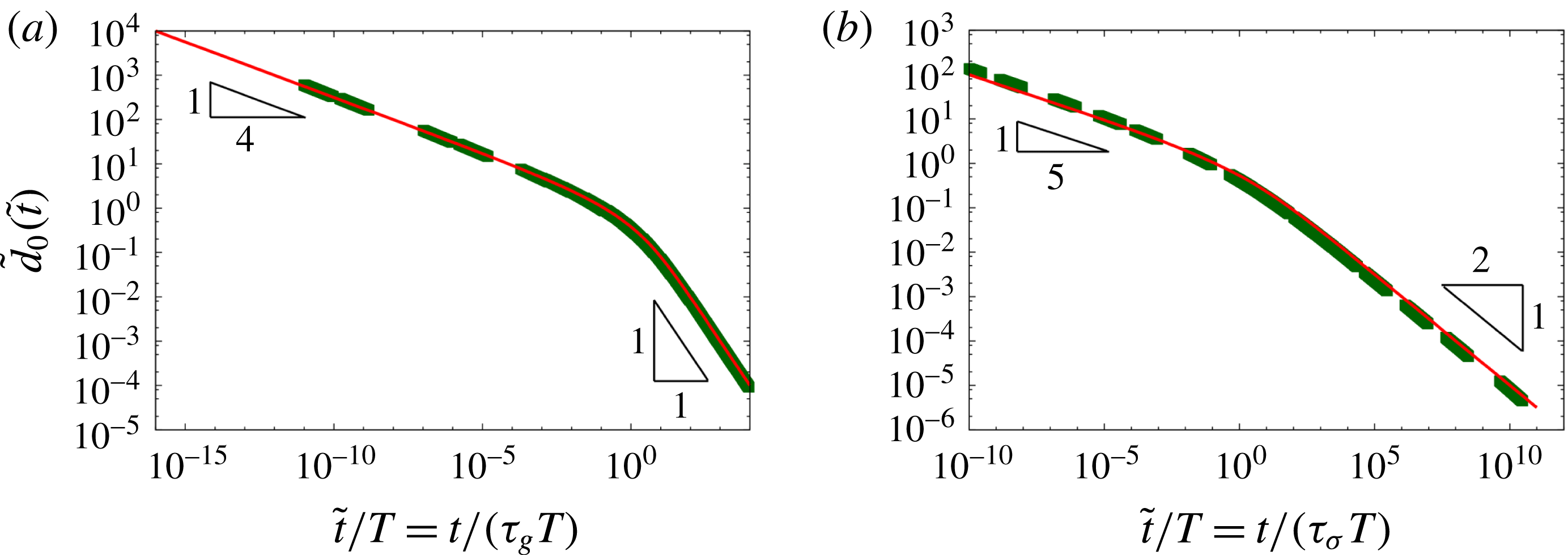
). To show that this is indeed the case, we plot in figure 15 the evolution of the non-dimensional excess drop height at the centre of the drop,
 $\tilde{d}_{0}(\tilde{t})=\tilde{d}(\tilde{r}=0,\tilde{t})$
, for all our simulations (but only using data from the regime when the drop displays a clearly defined power-law behaviour:
 $t>200~\text{s}$
for the large drop and
 $t>10^{5}~\text{s}$
for the small one; cf. figure 12). Figure 15 shows that many of the data points (indicated by symbols) come from a regime when the drop is still relatively thick relative to the thickness of the layer;
 $\tilde{d}_{0}\gg 1$
. The evolution of the excess drop height therefore follows a power-law behaviour with exponents
 $m=1/4$
or
 $m=1/5$
for ‘large’ and ‘small’ drops, respectively, over many decades. Drops that are deposited on thicker layers spread much more quickly and therefore reach the regime in which their excess height is much less than the film thickness (
 $\tilde{d}_{0}\ll 1$
; resulting in power-law exponents of
 $m=1$
and
 $m=1/2$
for ‘large’ and ‘small’ drops, respectively) within the duration of our computations. For such drops, the power-law exponents recorded at the fixed time of
 $10^{3}$
and
 $10^{5}~\text{s}$
for the ‘large’ and ‘small’ drops (as shown in figure 14) correctly captures their ultimate behaviour. Conversely, for drops spreading on thinner layers, the power-law exponent recorded at that time only provides a snapshot of their behaviour during their evolution towards the ultimate levelling behaviour.
Non-dimensional excess drop height
 $\tilde{d}_{0}$
as function of non-dimensional time
 $\tilde{t}/T$
for (a) the ‘large’ drop and (b) the ‘small’ drop, on a log–log scale. The constant
 $T$
is given by (4.12) where
 $k=1/2$
for the ‘large’ drop and
 $k=1/4$
for the ‘small’ one. The green points represent the computed data (for
 $t>200~\text{s}$
in (a), and
 $t>10^{5}~\text{s}$
in (b)), while the red lines show the predictions from the theoretical model, equation (4.11).

We note that Cormier et al. (Reference Cormier, McGraw, Salez, Raphaël and Dalnoki-Veress2012) derived the power-law behaviour reported above (for ‘small’ drops) not by appealing to King’s similarity solutions but by employing a volume-conservation argument that allows them to obtain an explicit prediction for the evolution of the excess drop height over the entire regime. We will now demonstrate that the argument can be extended to also describe the behaviour of ‘large’ drops. For this purpose we postulate that the non-dimensional excess drop height above the undeformed layer has the similarity form
 $$\begin{eqnarray}\tilde{d}(\tilde{r},\tilde{t})=\tilde{d}_{0}(t)\widetilde{{\mathcal{F}}}(\unicode[STIX]{x1D702}),\end{eqnarray}$$
where
 $\unicode[STIX]{x1D702}(\tilde{r},\tilde{t})$
is the similarity variable. Apart from a rescaling of
 ${\mathcal{F}}$
, so that
 $\tilde{d}_{0}(t)$
represents the non-dimensional excess height at the centre of the drop, this form of the solution is consistent with the similarity solutions specified in (4.6) and (4.7) for which
 $\unicode[STIX]{x1D702}$
has the form
 $\tilde{r}\,\tilde{t}^{-n}$
for some
 $n$
. Cormier et al. (Reference Cormier, McGraw, Salez, Raphaël and Dalnoki-Veress2012) report that in their experiments the interface shape appeared to be better described by a similarity variable of the form
 $$\begin{eqnarray}\unicode[STIX]{x1D702}=\frac{\tilde{r}}{[\tilde{t}\,(1+\tilde{d}_{0}(\tilde{t}))^{3}]^{k}},\end{eqnarray}$$
and they attributed the correction factor
 $(1+\tilde{d}_{0}(\tilde{t}))^{3}$
to a rescaling of time which accounts for the variable flow resistance which varies like
 $h^{-3}$
; see (4.1).
We now express the conservation of drop volume,
 $$\begin{eqnarray}2\unicode[STIX]{x03C0}\int _{0}^{\infty }d(r,t)r\,\text{d}r=V,\end{eqnarray}$$
in terms of the non-dimensional variables and represent the excess drop height
 $d$
in terms of (4.8) and (4.9) to obtain
 $$\begin{eqnarray}(\tilde{d}_{0}(\tilde{t}))^{1/(2k)}(1+\tilde{d}_{0}(\tilde{t}))^{3}=\frac{T}{\tilde{t}},\end{eqnarray}$$
where
 $$\begin{eqnarray}T=\left(\frac{V}{2\unicode[STIX]{x03C0}h_{\infty }^{3}\displaystyle \int _{0}^{\infty }\widetilde{{\mathcal{F}}}(\unicode[STIX]{x1D702})\unicode[STIX]{x1D702}\,\text{d}\unicode[STIX]{x1D702}}\right)^{1/(2k)}\end{eqnarray}$$
is a constant whose value depends on the form of the similarity solution
 $\widetilde{{\mathcal{F}}}(\unicode[STIX]{x1D702})$
, the film thickness
 $h_{\infty }$
, and the drop volume
 $V$
. Equation (4.11) predicts that
 $$\begin{eqnarray}\tilde{d}_{0}\sim \left\{\begin{array}{@{}ll@{}}t^{-2k/(6k+1)}\quad & \text{for }\tilde{d}_{0}\gg 1\\ t^{-2k}\quad & \text{for }\tilde{d}_{0}\ll 1.\end{array}\right.\end{eqnarray}$$
These limits agree with those from King’s exact similarity solutions if we choose
 $k=1/2$
for ‘large’ drops and
 $k=1/4$
for ‘small’ ones. More importantly, equation (4.11) provides an explicit prediction for the evolution of the excess drop height over the entire range of the drops’ evolution with just one fitting parameter, the constant
 $\unicode[STIX]{x1D6FD}=\int _{0}^{\infty }\widetilde{{\mathcal{F}}}(\unicode[STIX]{x1D702})\unicode[STIX]{x1D702}\,\text{d}\unicode[STIX]{x1D702}$
. The resulting prediction (using
 $\unicode[STIX]{x1D6FD}=1.65$
) is shown by the continuous lines in figure 15 and matches the computed data extremely well. Furthermore, the different power laws for
 $\tilde{d}_{0}\gg 1$
and
 $\tilde{d}_{0}\ll 1$
describe the system’s behaviour extremely robustly over many decades of the rescaled non-dimensional time,
 $\tilde{t}/T$
, with a rapid transition between the regimes when
 $\tilde{d}_{0}=O(1)$
and
 $\tilde{t}/T=O(1)$
.
Recall now that the plots of the rescaled drop shapes in figure 13 showed that the collapse of the data, based on the power-law exponents obtained from a fit to the computational results, worked least well for the intermediate layer thicknesses shown in figure 13(b,e). The explanation for this is that for these thicknesses the drop is in the transition between the two clearly defined power-law regimes shown in figure 15. The drops’ evolution can therefore not be described by a power law with a single, fixed exponent and an attempt to collapse the drop shapes by such a rescaling leads to noticeable discrepancies.
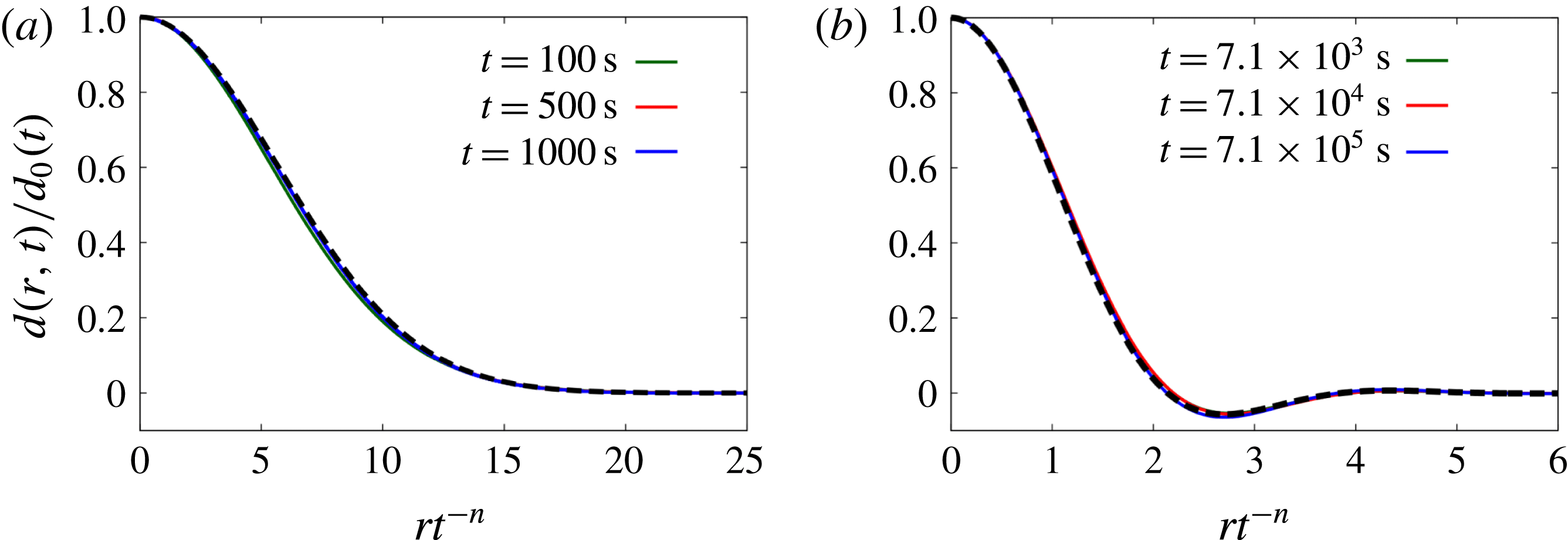
Conversely, drops deposited on sufficiently thick layers rapidly reach the ultimate spreading regime and their shapes are then well described by power-law-based similarity solutions. This is illustrated in figure 16 where we contrast the rescaled computational results (from the same time intervals as in figure 13, but for thicker layers) with the analytical solutions of the linear equations (4.5a,b
) that describe the drops’ ultimate spreading behaviour. For ‘large’ drops, the similarity solution is given by
 $\tilde{{\mathcal{F}}}_{g,\tilde{d}\ll 1}=\exp (-1/4\unicode[STIX]{x1D702}^{2})$
where
 $\unicode[STIX]{x1D702}=\tilde{r}\,\tilde{t}^{-1/2}$
; we refer to Backholm et al. (Reference Backholm, Benzaquen, Salez, Raphaël and Dalnoki-Veress2014) for the solution of (4.5b
) (for ‘small’ drops) in terms of hypergeometric functions.
Plots illustrating the self-similarity of the drop shapes for (a) the ‘large’ drop, (b) the ‘small’ drop, spreading on a layer of thickness
 $h_{\infty }=17~\text{mm}$
and
 $10~\unicode[STIX]{x03BC}\text{m}$
, respectively. The excess drop height
 $d(r,t)$
is normalised on its value at the centre of the drop,
 $d_{0}(t)$
, and the radial distances are rescaled on the similarity variable
 $rt^{-n}$
for the ultimate spreading regime for which
 $n=1/2$
for the ‘large’ drop and
 $n=1/4$
for the ‘small’ one. Here the radius and time are non-dimensionalised using the scalings of § 3.1. The solid lines represent the computed data, while the thick dashed black lines represent the analytical similarity solutions of (4.5a,b
).

5 Summary and conclusions
We employed experiments, numerical simulations and scaling analyses to study the axisymmetric spreading of drops of viscous, Newtonian fluids on a layer of the same fluid and contrasted their behaviour with that observed when such drops are deposited on dry substrates. Our experiments were performed with ‘large’ drops of glucose syrup, i.e. we operated in a regime of large Bond number where the overall dimensions of the drop are much larger than the capillary length, so that the behaviour of the drop is dominated by a balance between gravitational and viscous effects.
During the early stages of the drops’ evolution we identified three qualitatively different behaviours, depending on the thickness of the uniform fluid layer relative the typical size of the deposited drop. For very thin layers, the drop develops a steep spreading front, implying that there is a clearly defined drop radius whose value depends only weakly on the height at which it is measured. In this case, the spreading front introduces minimal perturbations to the fluid layer ahead of itself and the overall behaviour is very similar that observed for drops spreading on a dry substrate. For intermediate layer thicknesses, the leading edge of the spreading drop adopts a wedge-like profile and perturbs the pre-existing layer over a noticeable distance ahead of the drop radius. Finally, for thick layers, the drop sinks into the layer and causes noticeable upwelling in the fluid layer ahead of itself. This results in the formation of a transient bulge. Once this bulge has been levelled by gravity the leading edge of the drop again approaches a wedge-like profile, but with a much shallower angle than in the intermediate regime.
In all cases, the evolution of the drop ultimately reaches a regime within which the excess drop height and radius display a power-law behaviour over significant lengths of time while the drop shape evolves in a self-similar profile. The power-law exponents, measured at a fixed time, depend on the layer thickness, reflecting the fact that drops on thicker layers spread more quickly; the power-law exponents for drops spreading on very thin layers (where ‘thin’ has to be understood as thin relative to the excess drop height at the time when the exponents are determined) are close to (slightly larger) than those observed for drops spreading on dry substrates.
We performed additional computations in the small Bond number regime (i.e. for ‘small’ drops) where capillary effects play an important role, using parameter values that are appropriate for Cormier et al.’s (Reference Cormier, McGraw, Salez, Raphaël and Dalnoki-Veress2012) experiments with drops of molten polystyrene. Overall, the behaviour of these drops was found to be similar to that observed for ‘large’ drops. Specifically, when increasing the layer thickness the evolution of the drop shape passes from the ‘spreading’ to the ‘wedging’ regime before reaching a regime in which the drop ‘sinks’ into the layer. Furthermore, for both ‘small’ and ‘large’ drops the power-law exponents for the excess drop height and radius, measured at a fixed time, increase with the layer thickness. However, the power-law exponents for ‘small’ drops are generally smaller than for ‘large’ drops. This is similar to the trend observed in predictions based on scaling arguments for drops spreading on dry substrates.
A key observation is that, because the drops keep spreading indefinitely, their excess height will ultimately become less than the thickness of the layer they were deposited on. Beyond this point, the layer can no longer be regarded as thin and the drop’s evolution undergoes a final change to a universal late-time behaviour. We characterised the evolution towards this final spreading regime using a lubrication-theory-based model and showed that our computed data are well described by similarity solutions to suitably simplified equations. We note that Benzaquen et al. (Reference Benzaquen, Fowler, Jubin, Salez, Dalnoki-Veress and Raphael2014) performed a similar analysis and associated experiments to study the capillary-driven levelling of films in a two-dimensional geometry. Finally, we adapted an approach first used by Cormier et al. (Reference Cormier, McGraw, Salez, Raphaël and Dalnoki-Veress2012) to derive an explicit prediction for the temporal evolution of the excess drop height that captures the continuous evolution of the power-law exponents during the drop’s spreading.
Acknowledgements
The financial support of Mondelez International and the School of Mathematics (PhD Studentship) and the Leverhulme Trust (grant RPG-2014-081) is gratefully acknowledged. We would also like to thank the three referees for their insightful comments and constructive suggestions for improvement which motivated the analysis presented in § 4.5. Finally we thank Ashish Garg for alerting us to some typographical errors in the proofs of this paper.