


1. Introduction
Extreme waves are abnormally high structures that can happen unexpectedly on the ocean surface. These extreme events pose serious threats to the safety of ships, offshore platforms and coastal structures, and understanding their characteristics is therefore essential for robust marine design and ocean operations (Kharif & Pelinovsky Reference Kharif and Pelinovsky2003; Müller et al. Reference Müller, Garrett and Osborne2005).
Understanding the mechanism behind extreme-wave formation has long been a subject of interest in physics and mathematics. One major mathematical foundation of extreme waves in deep water has been established in the context of the nonlinear Schrödinger equation (NLS), which models the envelope process of a one-dimensional narrow-band wave field. We highlight here two soliton solutions of NLS as prototypes of extreme waves. The first one is the so-called Peregrine soliton (Peregrine Reference Peregrine1983), which is localised in both space and time and therefore represents a ‘rogue wave’ that appears and disappears in an abrupt manner. The Peregrine soliton has remarkably been observed in wave tank experiments (Chabchoub et al. Reference Chabchoub, Hoffmann and Akhmediev2011, Reference Chabchoub, Hoffmann, Onorato and Akhmediev2012) by carefully setting up of the boundary condition imposed by the wave maker. The second one is a spatially localised regular soliton that propagates with a persistent form, describing an extreme-wave group (with its envelope not changing) on the free surface. The regular soliton has also been observed in experiments (Slunyaev et al. Reference Slunyaev, Clauss, Klein and Onorato2013a ), including its associated soliton gas set-up (Chabchoub et al. Reference Chabchoub, Hoffmann, Onorato, Genty, Dudley and Akhmediev2013; Suret et al. Reference Suret2020; Fache et al. Reference Fache2024), although there seems to be less discussion of them in the context of extreme waves in deep-water conditions.
While the theory of solitons under NLS is highly idealistic, exploration of extreme waves in non-integrable higher-order nonlinear models is more relevant to realistic situations. The latter include, for example, studies of the modified nonlinear Schrödinger equation (MNLS) (Slunyaev et al. Reference Slunyaev, Pelinovsky, Sergeeva, Chabchoub, Hoffmann, Onorato and Akhmediev2013b ; Farazmand & Sapsis Reference Farazmand and Sapsis2017; Dematteis et al. Reference Dematteis, Grafke and Vanden-Eijnden2018) and fully nonlinear models (i.e. Euler equation of the free surface) (Brandini & Grilli Reference Brandini and Grilli2001; Clamond et al. Reference Clamond, Francius, Grue and Kharif2006; Ducrozet et al. Reference Ducrozet, Bonnefoy, Le Touzé and Ferrant2007; Chalikov Reference Chalikov2009; Slunyaev & Sergeeva Reference Slunyaev and Sergeeva2012; Slunyaev & Shrira Reference Slunyaev and Shrira2013; Xiao et al. Reference Xiao, Liu, Wu and Yue2013; Xia et al. Reference Xia, Ma, Dong, Zhang and Ma2021; Zhai et al. Reference Zhai, Klahn, Onorato and Fuhrman2025). Many of these studies track the extreme waves in the evolution of the wave field, and often attribute their formation to modulational instability (see also experimental studies in Onorato et al. Reference Onorato, Osborne, Serio, Cavaleri, Brandini and Stansberg2004, Reference Onorato2009; Shemer & Sergeeva Reference Shemer and Sergeeva2009).
In addition, Dematteis et al. (Reference Dematteis, Grafke and Vanden-Eijnden2018) explored a different and more challenging set-up using MNLS: taking random initial conditions satisfying Gaussian distributions, they estimate the exceedance probability of extreme waves (above high thresholds) at later times. The problem is made solvable through the large-deviation theory (LDT), which estimates the probability by identifying the most likely initial condition leading to an extreme wave exceeding the specified threshold. It is worthwhile mentioning that the extreme waves generated in all these studies are rogue-wave type with short duration, i.e. more like the scenario described by the Peregrine soliton. To the authors’ knowledge, there is so far no realisation of a persistent extreme-wave group (more like a regular soliton) in designed simulations using the models reviewed above (other than NLS).
In this paper, we demonstrate a new approach to generate extreme waves of flexible features in fully nonlinear wave models simulated by the high-order spectral (HOS) method. Our problem set-up is similar to that in Dematteis et al. (Reference Dematteis, Grafke and Vanden-Eijnden2018) where we have initial conditions with random phase distribution and aim to find both the extreme-wave event and the associated exceedance probability. The solution is enabled by coupling HOS to a generative artificial intelligence-based framework, hereafter named ‘GenWave’. This framework has previously been applied to the generation of extreme waves in linear and second-order wave theory (Xu & Maki Reference Xu and Maki2025), parametric roll in linear waves (Maki et al. Reference Maki, Park, Xu and Nam2026) and extreme roll motions in beam seas in combined linear wave and wind excitation (Seo et al. Reference Seo, Nam and Maki2026).
Specifically, GenWave is an iterative approach where in each iteration the phase ensemble is pushed toward those favouring extreme-wave generation, through a direct selection of desired phases followed by an expansion produced by a long–short-term-memory (LSTM) network. Although the general framework involves more simulations than the LDT-based approach, it does not require adjoint development (that is usually used with LDT) which makes it more suitable to couple with complex wave models (such as HOS) and potentially experiments. More importantly, with GenWave we are able to generate extreme waves of flexible features, including those spatially and temporally localised ones and those persistent groups travelling for a long distance whilst retaining their envelope shape.
The remainder of this paper is organised as follows. Section 2 provides a detailed problem statement on extreme-wave generation in fully nonlinear wave models. Section 3 describes the GenWave approach, including the iterative strategy, LSTM architecture and evaluation metrics, as well as a verification in linear waves. Section 4 presents the results regarding both the spatially and temporally localised rogue waves and persistent extreme-wave groups. The paper is concluded in § 5.
2. Problem statement
We consider a one-dimensional free surface of an inviscid and incompressible fluid with infinite depth, with its motion modelled by the Euler equation in Zakharov form (Zakharov Reference Zakharov1968)
 \begin{align} \frac {\partial \eta }{\partial t} = \left (1+\left |\frac {\partial \eta }{\partial x}\right |^2\right ) \left .\frac {\partial \varPhi }{\partial z}\right |_{z=\eta }-\frac {\partial \eta }{\partial x}\frac {\partial \varPhi ^s}{\partial x}, \\[-28pt] \nonumber \end{align}
 \begin{align} \frac {\partial \varPhi ^s}{\partial t}=-g\eta -\frac {1}{2}\left |\frac {\partial \varPhi ^s}{\partial x}\right |^2+\frac {1}{2}\left (1+\left |\frac {\partial \eta }{\partial x}\right |^2\right )\left (\left .\frac {\partial \varPhi }{\partial z}\right |_{z=\eta }\right )^2, \\[6pt] \nonumber \end{align}
where
 $x$
,
 $z$
are the horizontal, vertical coordinates and
 $t$
is time,
 $\eta (x,t)$
is the surface elevation,
 $\varPhi ^s(x,t) = \varPhi (x, z=\eta , t)$
is the velocity potential evaluated at the free surface, with
 $\varPhi (x,z,t)$
the velocity potential, and
 $g$
is the gravitational acceleration.
We set up an initial condition with random phases from a Joint North Sea Wave Project (JONSWAP) spectrum
 $S(\omega )$
with
 $\omega$
the angular frequency. Specifically, the initial surface elevation at
 $t=0$
is specified by
 \begin{equation} \eta (x, 0) = \sum _{i=1}^{N} a_i \cos (k_i x + \phi _i), \end{equation}
where
 $a_i = \sqrt {S(\omega _i) \boldsymbol{\cdot }\Delta \omega }$
, with
 $\Delta \omega$
the width of discretised bins in
 $\omega$
,
 $\omega _i$
the central value of each bin and where
 $k_i=\omega _i^2/g$
is the wavenumber. The phases
 $\phi _i$
are drawn from a uniform distribution
 $[-\pi , \pi )$
, independently for each
 $i$
.
Our goal is to identify a subset of initial conditions (i.e. choice of phases) that favours the generation of extreme waves of specified features, in particular a rogue wave at a design time and location, and a persistent extreme-wave group. We further define two metrics that characterise the features of the two desired types of extreme waves
 \begin{align} e_1 = \frac {\eta (x_d, t_d)}{H_s}, \\[-28pt] \nonumber \end{align}
 \begin{equation} e_2 = \frac {1}{T} \int _0^{T} \mathcal{H}\left ( \max _x \eta (x, t) - 1.25\,H_s \right ) \text{d}t, \end{equation}
where
 $e_1$
in (2.4) represents the surface elevation of a rogue wave at design location
 $x_d$
and time
 $t_d$
, normalised by the significant wave height
 $H_s$
;
 $e_2$
in (2.5) represents the fraction of time when the maximum surface elevation exceeds a threshold of
 $1.25H_s$
, with
 $\mathcal{H}(\boldsymbol{\cdot })$
a Heaviside step function and
 $T$
the duration of temporal window. Mathematically, we aim to find initial phases which maximise metrics
 $e_1$
and
 $e_2$
, as well as the associated probabilities of exceedance (POEs),
 $P(e_1\gt z)$
and
 $P(e_2\gt z)$
, for large
 $z$
.
It is worth setting out at this point the two criteria in common use to declare an individual wave to be a ‘rogue’ wave. The first is based on the crest-to-trough wave height
 $H$
. The threshold
 $H\gt 2H_s$
is the most widely adopted (Michel et al. Reference Michel, Bonnefoy, Ducrozet and Falcon2022), where
 $H_s=4\sigma$
is the significant wave height and
 $\sigma$
is the standard deviation of the surface elevation, and individual events well above it are reported in simulations of random sea states, for instance
 $H_{max }/H_s=2.25$
in Onorato et al. (Reference Onorato, Osborne, Serio and Bertone2001). The second criterion is based on the crest elevation alone,
 $\eta _c\gt 1.25H_s$
, equivalently
 $\eta _c\gt 5\sigma$
(Michel et al. Reference Michel, Bonnefoy, Ducrozet and Falcon2022; Zhai et al. Reference Zhai, Klahn, Onorato and Fuhrman2025). The two thresholds are not interchangeable. They measure different quantities, and the crest–trough asymmetry of a nonlinear wave field makes the relation between them dependent on the sea state, so that a wave satisfying one criterion need not satisfy the other. In this work we adopt the crest-based criterion
 $\eta _c\gt 1.25H_s$
, which is the natural choice when the quantity of interest is the elevation reached at a prescribed point in space and time, and we report the wave height
 $H$
separately wherever the comparison with the
 $H\gt 2H_s$
criterion is useful.
Before moving on to the description of the GenWave framework, we summarise the numerical details of the problem. The system is solved numerically using the HOS method (Dommermuth & Yue Reference Dommermuth and Yue1987; West et al. Reference West, Brueckner, Janda, Milder and Milton1987) with a nonlinearity order
 $M=3$
(which incorporates modulational instability), in a computational domain of
 $[-\pi , \pi )$
discretised by 256 grid points, corresponding to
 $N=64$
modes after de-aliasing. A dissipation model is incorporated in HOS following Xiao et al. (Reference Xiao, Liu, Wu and Yue2013) to represent wave breaking and ensure the stability of the simulations. The initial JONSWAP spectrum
 $S(\omega )$
is chosen to be associated with a significant wave height
 $H_s = 3.0$
m, a peak period
 $T_p = 8.0$
s and a peak enhancement factor
 $\gamma = 6.0$
. The parameters
 $x_d$
,
 $t_d$
in (2.4) and
 $T$
in (2.5) will be specified later in § 4.
3. Methodology
This section presents the GenWave framework which integrates the nonlinear wave model with machine learning to efficiently generate extreme-wave events. The framework employs LSTM networks to learn optimal phase combinations from progressively refined datasets through an iterative strategy. We first describe the overall framework, followed by the architecture of LSTM. Then, we verify its effectiveness in the setting of linear waves.
3.1. GenWave framework
In the GenWave framework, we adopt an iterative refinement strategy, as illustrated in figure 1. The core idea is to progressively bias the generative model toward phase configurations that produce increasingly extreme-wave events through successive rounds of ranking, selecting and retraining.
Schematic of the GenWave framework.

In iteration 0, an ensemble of
 $N_{\text{s}}$
phase vectors
 $\boldsymbol{\phi } = (\phi _1, \phi _2, \ldots , \phi _N)$
is drawn from a uniform and independent distribution
 $\phi _k \sim \mathcal{U}[-\pi , \pi )$
for
 $k = 1, 2, \ldots , N$
. Each
 $\boldsymbol{\phi }$
is then evaluated through HOS simulation, resulting in
 $N_s$
values of the evaluation metric (
 $e_1$
or
 $e_2$
defined in (2.4) and (2.5)). Three procedures are then followed in each iteration.
-
(i) Ranking and selection: the
 $N_s$
phase vectors
$\boldsymbol{\phi }$
are ranked in descending order according to the evaluation metric. Only the top
$N_s/q$
phase vectors
$\boldsymbol{\phi }$
which lead to the most extreme values of the evaluation metric are retained as training data for the LSTM network. A detailed description of the LSTM network architecture for GenWave is presented in Xu & Maki (Reference Xu and Maki2025).
-
(ii) Training of LSTM: the LSTM network is trained on the selected phase vectors
$\boldsymbol{\phi }$
to learn the conditional probability distribution
$P_\theta (\phi _k \mid \phi _1, \ldots , \phi _{k-1})$
for the phase component
$\phi _k$
given the preceding phase angles. The GenWave architecture is inspired by language models that estimate the likelihood of sequential data. Since such models operate on discrete tokens, each continuous phase
$\phi _k$
is discretised into
$K$
uniform bins over the range
$[-\pi , \pi )$
. The chain rule of probability then decomposes the joint distribution into a product of conditional probabilities(3.1)where
\begin{equation} P_\theta (\boldsymbol{\phi }) = P_\theta (\phi _1) \prod _{k=2}^{N} P_\theta (\phi _k \mid \phi _1, \ldots , \phi _{k-1}), \end{equation}
$\theta$
denotes the learned network parameters.
-
(iii) Generation of new phase vectors: using autoregressive sampling from the trained LSTM network,
$N_{\text{s}}(1-1/q)$
new phase vectors
$\boldsymbol{\phi }$
are generated. These newly generated samples are combined with the
$N_s/q$
top-performing phase vectors
$\boldsymbol{\phi }$
retained from the previous iteration to form a complete ensemble of
$N_s$
phase vectors for the next iteration.


This iterative process continues, with each iteration using the
 $N_s$
phase vectors
 $\boldsymbol{\phi }$
(both LSTM generated and retained samples) as input to repeat the three steps. After multiple iterations, the ensemble becomes increasingly concentrated in regions of the phase space that produce extreme-wave events. Throughout this study, we use
 $N_s = 10{\,}000$
,
 $q = 4$
and
 $K = 60$
.
The use of LSTM networks offers a different sampling strategy from traditional rare-event methods such as subset simulation (Au & Beck Reference Au and Beck2001) and adaptive multilevel splitting (Cérou & Guyader Reference Cérou and Guyader2007). While these methods generate new samples through local perturbations of existing high-performing samples (e.g. via Markov chain Monte Carlo or particle mutation), the LSTM directly learns
 $P_\theta (\phi _k \mid \phi _1, \ldots , \phi _{k-1})$
from the top-performing samples, capturing dependencies among phases across the entire frequency range.
To validate the statistical accuracy of GenWave, we compare the POE obtained from the generated samples with direct Monte Carlo sampling (MCS) results. For GenWave with iterative refinement, wave fields generated at iteration
 $k$
represent conditional samples that have passed through
 $k$
successive selection stages. Under the assumption that each iteration independently selects the top
 $N_s/q$
phase vectors, the probability of this conditioning event is
 $(1/q)^k$
. Therefore, for
 $N_s$
values of an evaluation metric generated from iteration
 $k$
sorted in descending order, the scaled POE is
 \begin{equation} P(e_{(i)}\gt z) = \frac {1}{q^k} \boldsymbol{\cdot }\frac {i}{N_s+1}, \quad i = 1, \ldots , N_s. \end{equation}
Note that the method employed here to compute the POE for GenWave is an approximation. This is because the LSTM network perturbs the distribution of the selected
 $1/q$
ensemble in each iteration, meaning that the
 $(1/q)^k$
scaling factor becomes approximate rather than exact. However, as demonstrated in §§ 3.2 and 4, this approximation provides sufficient accuracy for the purposes of this study. A more rigorous calculation would require determining the joint probability distribution of the phases from the learned LSTM network and employing importance sampling techniques to account for the distributional shift introduced by the LSTM network. This represents an avenue for future improvement of the POE estimation methodology.
For the parameters used here,
 $N_s=10{\,}000$
and
 $q=4$
, the initial ensemble requires
 $N_s$
HOS simulations and each subsequent iteration requires
 $N_s(1-1/q)=7500$
new HOS simulations. Thus, the cumulative number of HOS evaluations through iteration
 $k$
is
 $C_k=10{\,}000+7500k$
. The nominal lower end of the scaled POE curve at that iteration is
 $(1/q)^k/(N_s+1)$
. Consequently, the computational cost grows linearly with
 $k$
, or logarithmically with the inverse nominal POE level, whereas direct Monte Carlo requires
 $O(1/P)$
samples to observe an event of probability
 $P$
.
3.2. Verification in linear waves
Before applying GenWave to nonlinear waves, we first verify its effectiveness in generating extreme waves in the linear wave model using (2.3). Here, the parameters for
 $S(\omega )$
are set as
 $H_s=3.0$
m,
 $T_p=8.0$
s and
 $\gamma =1.0$
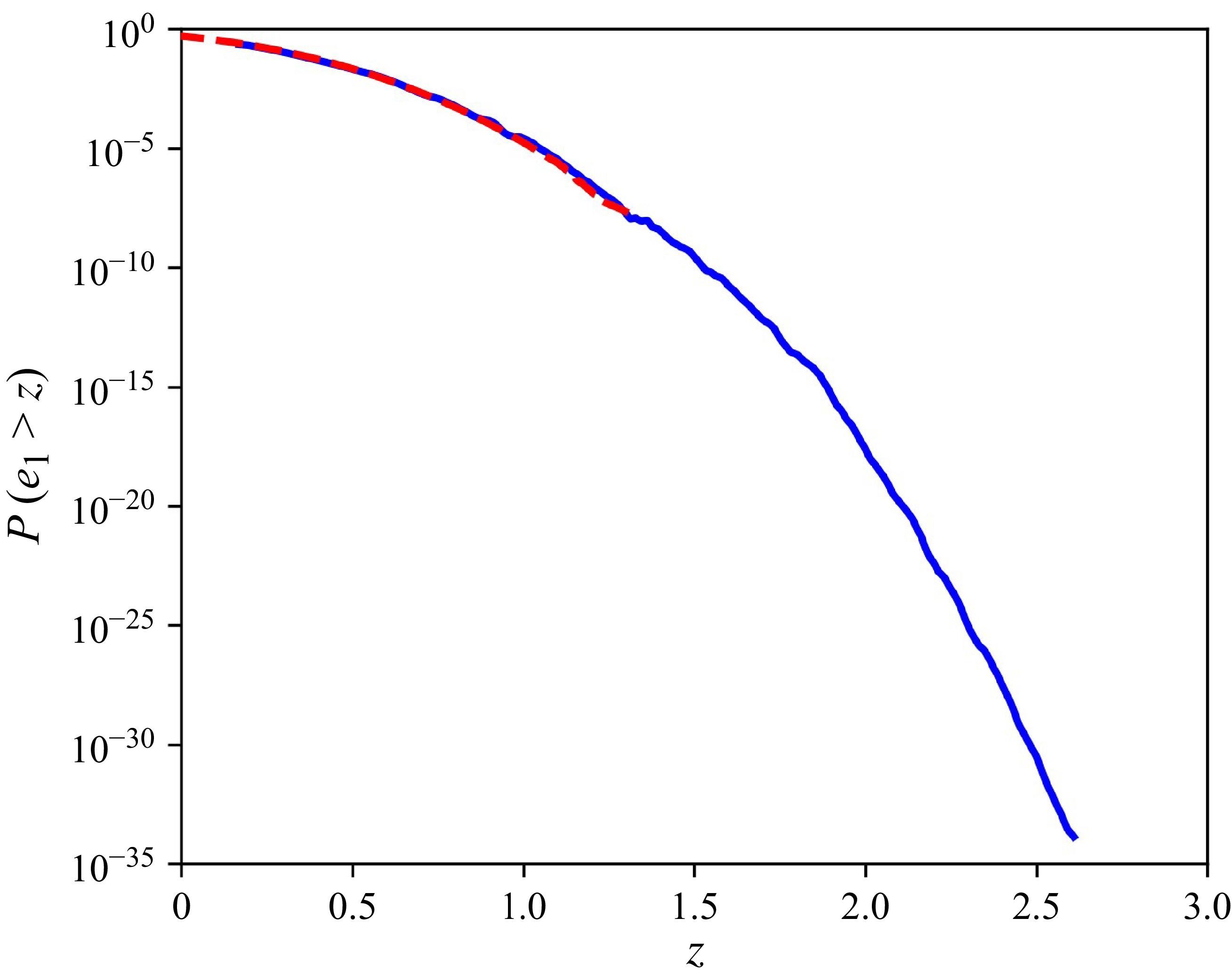
. Figure 2 presents
 $P(e_1\gt z)$
as a function of
 $z$
for linear waves. The comparison between the GenWave and MCS-based POE demonstrates good agreement, confirming that GenWave enables exploration of the heavy-tail region of the distribution with substantially fewer simulations. GenWave extends the nominal lower end of
 $P(e_1\gt z)$
to approximately
 $10^{-35}$
with 50 iterations (385 000 HOS simulations), a regime that would require an impractically large number of MCS samples to explore directly. Furthermore, the results confirm that GenWave is capable of generating waves exhibiting extreme elevations at the design point within the linear wave regime. Based on these findings, the generation of extreme waves with flexible features in nonlinear wave fields is pursued in § 4.
Value of
 $P(e_1\gt z)$
as a function of
 $z$
: MCS with
 $5\times 10^7$
simulations (red dashed), and GenWave results across 50 iterations (blue solid).

4. Results
4.1. Generation of rogue waves based on metric
$e_1$

We first present results of rogue wave generation based on the metric
 $e_1$
in (2.4) with
 $x_d=0$
and
 $t_d=50\,T_p$
. Figure 3 shows the evolution of the metric
 $e_1$
as the number of iteration increases. Specifically, we plot the ensemble mean, ensemble maximum and standard deviation at each iteration. We see a rapid increase in the mean and maximum values of the metric
 $e_1$
, and a relatively stationary standard deviation in the iteration process. In terms of the mean value, it increases from close to
 $0$
at iteration 0 to
 $1.585$
at iteration 20, which is accompanied by a maximum value of
 $1.953$
. While it is possible to further improve the metric
 $e_1$
with more iterations, we practically stop at iteration 20, which already serves the purpose of the paper.
Evolution of the metric
 $e_1$
over GenWave iterations: ensemble maximum (red solid
 $\circ$
), ensemble mean (blue dashed
 $\square$
) and standard deviation (green dotted
 $\triangle$
) at each iteration.

Wave ensembles generated by GenWave using the metric
 $e_1$
; (a, c, e) time history of
 $\eta (x_d, t)$
and (b, d, f) spatial profiles
 $\eta (x, t_d)$
at iterations 0, 10 and 20, respectively. Shown are 1000 individual ensemble members (grey), the ensemble member with maximum
 $e_1$
(red solid) and the mean of the ensembles (blue dashed). The peak wavelength
 $\lambda _p$
is defined as
 $gT_p^2/2\pi$
.

Figure 4. Long description
Panel A: A line graph showing the time history of wave ensembles at iteration 0. The x-axis is labeled t/Tp and ranges from 40 to 60. The y-axis is labeled η(xd, t)/Hs and ranges from -1.5 to 2.5. The graph includes 1000 individual ensemble members in grey, the ensemble member with maximum in red solid, and the mean of the ensembles in blue dashed. Panel B: A line graph showing the spatial profiles of wave ensembles at iteration 0. The x-axis is labeled x/λp and ranges from -7 to 7. The y-axis is labeled η(xd, t)/Hs and ranges from -1.5 to 2.5. The graph includes 1000 individual ensemble members in grey, the ensemble member with maximum in red solid, and the mean of the ensembles in blue dashed. Panel C: A line graph showing the time history of wave ensembles at iteration 10. The x-axis is labeled t/Tp and ranges from 40 to 60. The y-axis is labeled η(xd, t)/Hs and ranges from -1.5 to 2.5. The graph includes 1000 individual ensemble members in grey, the ensemble member with maximum in red solid, and the mean of the ensembles in blue dashed. Panel D: A line graph showing the spatial profiles of wave ensembles at iteration 10. The x-axis is labeled x/λp and ranges from -7 to 7. The y-axis is labeled η(xd, t)/Hs and ranges from -1.5 to 2.5. The graph includes 1000 individual ensemble members in grey, the ensemble member with maximum in red solid, and the mean of the ensembles in blue dashed. Panel E: A line graph showing the time history of wave ensembles at iteration 20. The x-axis is labeled t/Tp and ranges from 40 to 60. The y-axis is labeled η(xd, t)/Hs and ranges from -1.5 to 2.5. The graph includes 1000 individual ensemble members in grey, the ensemble member with maximum in red solid, and the mean of the ensembles in blue dashed. Panel F: A line graph showing the spatial profiles of wave ensembles at iteration 20. The x-axis is labeled x/λp and ranges from -7 to 7. The y-axis is labeled η(xd, t)/Hs and ranges from -1.5 to 2.5. The graph includes 1000 individual ensemble members in grey, the ensemble member with maximum in red solid, and the mean of the ensembles in blue dashed.
We further plot the spatial profile
 $\eta (x, t_d)$
and time history
 $\eta (x_d, t)$
of the waves obtained at iterations 0, 10 and 20 in figure 4, again demonstrating the increased metric
 $e_1$
with iterations. In iteration 20, the ensemble-mean profile has a rogue-wave structure with a local crest-to-trough height of
 $H=2.262\,H_s$
(see figure 4
f). This ensemble-mean profile satisfies both criteria stated in § 2: its crest elevation at the design point is
 $\eta (x_d,t_d)=1.585\,H_s$
, i.e.
 $e_1=1.585$
, above the crest threshold of
 $1.25\,H_s$
, and its local crest-to-trough height is
 $2.262\,H_s$
, above the height threshold of
 $2H_s$
. The most extreme member of the same ensemble reaches
 $e_1=1.953$
. The time history
 $\eta (x_d, t)$
at iteration 20 exhibits an asymmetric pattern (see figure 4
e), with the front sister wave lower than the trailing sister wave. This asymmetry is consistent with the experimental observations reported by Dematteis et al. (Reference Dematteis, Grafke, Onorato and Vanden-Eijnden2019), which supports the physical plausibility of the extreme waves generated by the present approach.
The POE
 $P(e_1\gt z)$
, as a function of
 $z$
computed from (3.2), is shown in figure 5. We show the values of
 $P(e_1\gt z)$
from direct MCS for a range that is practical to compute. We see good agreement of the two approaches, with the GenWave result extending to much lower probabilities at much larger z.
The growth of the ensemble statistics in figure 3 is itself evidence that the network is generating phase vectors concentrated in the rare-event region, rather than sampling independently of the retained ensemble. Under the near-Gaussian prior the metric
 $e_1$
has a standard deviation of
 $\sigma /H_s=1/4$
, the value found at iteration 0, so that an independent draw would exceed the iteration-20 ensemble mean of
 $e_1=1.585$
with a probability of order
 $10^{-10}$
and a batch of 7500 such draws would be expected to contain none. Moreover, even if all 2500 retained members were at the observed iteration-20 maximum of
 $e_1=1.953$
, their contribution to the mean of the full 10 000-member ensemble would be only 0.488. The observed iteration-20 ensemble is therefore incompatible with the newly generated samples being independent prior draws. What this does not establish is that the ensemble at iteration
 $k$
remains representative of the prior conditioned on the selection events, which is the assumption behind (3.2) and the reason the resulting POE is approximate.
Value of
 $P(e_1\gt z)$
as a function of
 $z$
: MCS with
 $10^4$
simulations (red dashed), and GenWave results across 20 iterations (blue solid).

We finally study the envelope process by taking a Hilbert transform in space on
 $\eta (x,t)$
for
 $t_d-10T_p\lt t\lt t_d+10T_p$
, which provides us with the amplitude of the wave envelope
 $A(x,t)$
(see figure 6 for
 $A(x,t)$
at three choices of
 $t$
). An animation of the process with respect to
 $\eta (x,t)$
is included in the supplemental materials. Furthermore, in figure 7, we plot
 $A(x,t_d)$
and
 $A(x_d,t)$
compared with the solution of a Peregrine soliton, with the latter obtained by setting parameters
 $\psi _0=A(x_d, t_d)/3$
to match the amplitude of the wave envelope at
 $(x_d, t_d)$
, and
 $k_0=(2\pi /T_p)^2/g$
that corresponds to the peak of the wavenumber in
 $S(\omega )$
(see Appendix A for parameters in the solution of a Peregrine soliton). We find reasonable agreement for both the spatial and time histories around
 $x_d$
and
 $t_d$
in figure 7. The discrepancy, as also observed in Dematteis et al. (Reference Dematteis, Grafke, Onorato and Vanden-Eijnden2019), is to be expected due to the application of the fully nonlinear wave model, which captures much more physics than the NLS.
Spatial profiles of
 $A(x,t)$
, where
 $t=t_d-10\,T_p$
(red solid),
 $t_d$
(blue dashed) and
 $t_d+10\,T_p$
(green dotted) from GenWave at iteration 20.

Comparison of
 $A(x,t_d)$
from GenWave at iteration 20 (red solid) and the solution of the Peregrine soliton (blue dashed): (a) spatial profile, (b) time history.

4.2. Generation of extreme-wave groups based on metric
$e_2$

We now turn to the generation of persistent extreme-wave groups based on the metric
 $e_2$
. We start by pointing out that, for more efficient iterations in GenWave to find the persistent extreme-wave group, it is beneficial to slightly modify (2.5) into
 \begin{equation} e_2 = \frac {\eta (0, 0)}{H_s}+w\boldsymbol{\cdot }\frac {1}{T} \int _0^{T} \mathcal{H}\left ( \max _x \eta (x, t) - 1.25\,H_s \right ) \text{d}t, \end{equation}
where
 $w$
is a large coefficient, here chosen as
 $50$
;
 $T=100\,T_p$
is the time window used in the GenWave training process, but the finally obtained extreme-wave group lasts for much longer time. The first term is adopted in (4.1) because it facilitates an effective growth of the metric
 $e_2$
in the first few iterations, which then triggers the rapid growth of the full term, until finally the value of the metric
 $e_2$
is dominated by the second term due to the large
 $w$
. The evidence of this process is presented in this section.
In figure 8 we show the evolution of metric
 $e_2$
with iterations using the same statistical measure as in figure 3 for metric
 $e_1$
. We see an increase in metric
 $e_2$
with the iterations, which reaches above 35 at iteration 20. Since
 $w$
is chosen to be 50, one might attempt to argue that the wave group obtained has approximately 15/50 = 30 % of time below the threshold of
 $1.25\,H_s$
. This is in fact not accurate because, for a wave group with fluctuating
 $\eta (x, t)$
, it is more robust to use
 $\max _x A(x, t)$
, where
 $A(x, t)$
is the amplitude of the wave envelope, instead of
 $\max _x \eta (x, t)$
in the group to measure its elevation. The measure of the envelope process is presented in figures 11 and 12.
Evolution of the metric
 $e_2$
over GenWave iterations: ensemble maximum (red solid
 $\circ$
), ensemble mean (blue dashed
 $\square$
) and standard deviation (green dotted
 $\triangle$
) at each iteration.

To provide more insight into the first term in (4.1), we plot the ensemble mean of the first and second terms in figure 9, as functions of the number of iterations. We clearly see that, in the first 5 iterations, the growth of metric
 $e_2$
is dominated by the growth of the first term. After iteration 5, the growth of the second term is triggered and dominates the entire metric
 $e_2$
. Physically, this can be interpreted by the fact that the persistent extreme-wave group scenario is rarer than simply a rogue wave. If we use only the second term of the metric
 $e_2$
in GenWave, it is difficult to find waves that are both high and persistent at initial iterations. The more practical way is to use the composite form of the metric
 $e_2$
as in (4.1), where GenWave attempts to first find some high waves, among which it continues to search for persistent wave groups.
Ensemble mean of each term in the metric
 $e_2$
over GenWave iterations: first term (red solid
 $\circ$
) and second term (blue dashed
 $\square$
) in (4.1).

Spatial profiles of
 $\eta (x,t)$
, where
 $t$
is at (a)
 $48\,T_p$
, (b)
 $50\,T_p$
, (c)
 $52\,T_p$
and (d)
 $54\,T_p$
from GenWave at iteration 20.

We next plot the profile of the extreme-wave groups
 $\eta (x,t)$
for
 $t$
=
 $48\,T_p, 50\,T_p, 52\,T_p$
and
 $54\,T_p$
obtained at iteration 20 in figure 10. An animation of
 $\eta (x,t)$
is included in the supplemental materials. We see that the persistent structure propagates through the domain, as desired. To further demonstrate the persistence of wave groups, we compute the evolution of the wave group for longer time than
 $T=100\,T_p$
used in (4.1). We also calculate
 $\max _x\eta (x,t)$
and
 $\max _x A(x,t)$
, with the two quantities plotted as a function of
 $t$
in figure 11. We find that, even though
 $\max _x\eta (x,t)$
can fluctuate below the threshold of
 $1.25\,H_s$
,
 $\max _x A(x,t)$
stays consistently above this threshold. Although the metric
 $e_2$
used in GenWave is only for a time period of
 $T=100\,T_p$
, the achieved extreme-wave group in fact stays above the threshold for a much longer time period of at least
 $200\,T_p$
. For an even longer simulation, the wave group will eventually diminish inevitably because of the dissipation in the HOS solver, which is practically needed to maintain the stability of the computation.
Time history of
 $\max _x \eta (x, t)/H_s$
(red solid) and the
 $\max _x A(x, t)/H_s$
(blue dashed) from GenWave at iteration 20. The threshold of
 $1.25$
is marked by a green dotted line.

Space–time diagrams of the envelope amplitude
 $A(x,t)/H_s$
from GenWave at iteration 20: (a) fully nonlinear evolution (
 $M=3$
) and (b) linear evolution of the same initial condition. The design point is at the centre of the periodic domain.

The space–time structure of the wave group is shown in figure 12. Under the fully nonlinear evolution the envelope propagates as a single straight streak that recirculates through the periodic domain over the entire time period of
 $200\,T_p$
. The measured speed is
 $1.060\,c_g$
, where
 $c_g=\omega _p/(2k_p)$
is the linear group velocity at the spectral peak, with
 $\omega _p=2\pi /T_p$
and
 $k_p=\omega _p^2/g$
(identical to the carrier parameters
 $\omega _0$
and
 $k_0$
defined in § 4.1). The amplitude of the group is maintained at
 $A_{max }\approx 1.6\,H_s$
throughout. In contrast, the linear evolution of the same initial condition gradually disperses, its envelope maximum decaying to
 $0.75\,H_s$
by the end of the simulation. The persistence of the group is thus entirely a nonlinear effect. The measured kinematics also explains the oscillation of
 $\max _x\eta (x,t)$
observed in figure 11. Since the crest travels at the phase speed
 $c_p=\omega _p/k_p\approx 2c_g$
while the envelope translates at the measured
 $1.060\,c_g$
, the crests slide through the group and the crest/envelope alignment recurs with a predicted period
 $2\pi /(\omega _p-1.060\,k_pc_g)\approx 2.1\,T_p$
. This is consistent with the measured period of
 $2.07\,T_p$
for the red curve in figure 11, corresponding to approximately 9.7 cycles in every
 $20\,T_p$
of the record.
Wavenumber–frequency energy density
 $E(k,\omega )$
in (4.2) (logarithmic scale, normalised by its maximum, with darker blue indicating higher energy) from GenWave at iterations (a) 5, (b) 10 and (c) 20, each averaged over the ensemble, and (d) for the analytic NLS envelope soliton with
 $\psi _0$
matched to the amplitude of the group. The black dashed curve is the linear dispersion relation
 $\omega =\sqrt {gk}$
, and the red dash-dotted line is the coherent branch
 $\omega =\omega _c+V(k-k_p)$
fitted to the spectral ridge over
 $0.7\leqslant k/k_p\leqslant 1.3$
, with
 $V=1.040\,c_g$
,
 $1.055\,c_g$
,
 $1.080\,c_g$
and
 $1.005\,c_g$
in (a)–(d) and
 $\omega _c=1.01\,\omega _p$
,
 $1.01\,\omega _p$
and
 $1.02\,\omega _p$
in (a)–(c), respectively.

Figure 13. Long description
Panel A: A scatter plot showing the wavenumber-frequency energy density at iteration 5. The x-axis is labeled k/kp and the y-axis is labeled ω/ωp. The color scale on the right indicates the logarithmic energy density, with darker blue representing higher energy. A black dashed curve represents the linear dispersion relation, and a red dash-dotted line represents the coherent branch. Panel B: A scatter plot similar to Panel A but at iteration 10. Panel C: A scatter plot similar to Panel A but at iteration 20. Panel D: A scatter plot showing the wavenumber-frequency energy density for the analytic NLS envelope soliton. The axes and color scale are the same as in the previous panels.
The kinematics of the group is further characterised in the wavenumber–frequency domain in figure 13, which shows the energy density
 \begin{equation} E(k,\omega ) = \left | \int _0^{100\,T_p}\!\!\int _{-L/2}^{L/2} \eta (x,t)\,W(t)\, e^{-\mathrm{i}(kx-\omega t)}\,\mathrm{d}x\,\mathrm{d}t \right |^2, \end{equation}
where
 $L=15\lambda _p$
is the length of the periodic domain and
 $W(t)$
a Hann window. Figure 13(a–c) shows
 $E(k,\omega )$
from GenWave at iterations 5, 10 and 20, respectively, and figure 13(d) shows the same transform applied to the analytic NLS envelope soliton of Appendix A. This spatio-temporal representation separates free waves, which lie on (or in the vicinity of) the linear dispersion relation
 $\omega =\sqrt {gk}$
, from bound waves, i.e. components away from the dispersion relation that are generated by non-resonant nonlinear interactions and travel with the waves that generate them rather than at their own free-wave speed (Zhang & Pan Reference Zhang and Pan2022).
Two observations follow from figure 13. The first is that the wave group travels as a coherent structure rather than as a dispersive superposition of free waves, and the second is that the speed of that structure can be measured directly from the spectrum and compared with the group velocity predicted by NLS. The low-wavenumber content follows the linear dispersion relation, whereas the energetic band around and above the spectral peak is aligned instead with the straight line
 \begin{equation} \omega = \omega _c + V\,(k-k_p), \end{equation}
which we refer to as the coherent branch. When the spectral content lies on such a line, the surface elevation can be written as a fixed profile in the frame
 $x-Vt$
multiplied by a carrier oscillating at
 $\omega _c-Vk_p$
, so that the envelope of the group propagates without change of form at the speed
 $V=\mathrm{d}\omega /\mathrm{d}k$
while the individual crests continue to travel at their own phase speed. The sliding of the crests through the envelope noted above in figure 11 is exactly this difference between the two speeds. Free waves on the dispersion relation
 $\omega =\sqrt {gk}$
behave differently, since their group velocity varies with
 $k$
and an initially localised packet therefore spreads.
The two parameters of (4.3) are measured directly from each spectrum in figure 13. The energetic part of the spectrum occupies the band
 $0.7\,k_p\leqslant k\leqslant 1.3\,k_p$
, which contains nine discrete wavenumbers at the resolution
 $\Delta k=2\pi /L=k_p/15$
of the periodic domain. At each of these wavenumbers we locate the ridge frequency
 $\omega _r(k)=\arg \max _{\omega }E(k,\omega )$
on the frequency grid
 $\Delta \omega =2\pi /(100\,T_p)=\omega _p/100$
set by the analysis window. The speed
 $V$
is the slope of a least-squares straight-line fit of
 $\omega _r(k)$
across this band, and the branch is anchored at the ridge frequency of the spectral peak,
 $\omega _c=\omega _r(k_p)$
. Throughout,
 $V$
is compared with the linear group velocity of the spectral peak in deep water,
 $c_g=(\mathrm{d}\omega /\mathrm{d}k)\vert _{k_p}=(1/2)\sqrt {g/k_p}$
.
Comparison of spatial profiles of
 $A(x,t_d)$
from GenWave at iteration 20 (red solid) and the solution of the regular soliton (blue dashed).

The two parameters carry different information, and the fitted values are given in the caption of figure 13. The anchor
 $\omega _c$
is the carrier frequency of the group. It lies
 $1$
%–
 $2\,\,\%$
above
 $\omega _p$
and grows with the iterations, which is the magnitude of the carrier frequency shift
 $(k_p\psi _0)^2/4\approx 2\,\%$
that NLS predicts at the measured group steepness
 $k_p\psi _0\approx 0.28$
(Appendix A). The slope
 $V$
is the speed at which the group travels. It grows from
 $1.040\,c_g$
at iteration 5 to
 $1.055\,c_g$
at iteration 10 and
 $1.080\,c_g$
at iteration 20, tracking the growth of the amplitude of the groups, and it agrees with the propagation speed of
 $1.060\,c_g$
measured independently from the space–time diagram of figure 12. The Euler and NLS descriptions agree on the first parameter and differ on the second. The cubic nonlinearity of the NLS shifts the carrier frequency, and the shift is therefore carried by the reconstruction (A3) used for figure 13(d), but the envelope of the leading-order NLS soliton still translates at exactly the linear group velocity
 $c_g$
, whereas the group generated in the fully nonlinear model travels
 $4$
%–
 $8\,\%$
faster than
 $c_g$
, an excess of the order of the finite-amplitude correction at the measured steepness.
Two further branches appear in figure 13(a–c), lying away from the dispersion relation. These are the bound waves generated by the group, and they correspond to the two mechanisms identified by Zhang & Pan (Reference Zhang and Pan2022): a superharmonic branch along
 $\omega =\sqrt {2gk}$
, formed by the second harmonics
 $(2\omega , 2k)$
of the free waves, and a low-frequency branch through the origin with slope
 $V$
, formed by the difference interactions
 $(\omega _1-\omega _2, k_1-k_2)$
among the components of the group. Their combined energy grows from approximately
 $0.5\,\%$
of the total at iteration 5 to
 $1.2\,\%$
at iteration 20, so that the group becomes progressively more nonlinear as GenWave drives it toward larger amplitude.
Value of
 $P(e_2\gt z)$
as a function of
 $z$
: MCS with
 $5\times 10^4$
simulations (red dashed), and GenWave results across 20 iterations (blue solid).

The panel for the analytic NLS soliton, figure 13(d), completes the comparison in two ways. It first tells us how much of the measured excess in
 $V$
we should believe. The envelope of the reconstruction (A3) translates at exactly
 $c_g$
, and applying the same fit to its spectrum returns
 $V=1.005\,c_g$
, so that a known speed is recovered to within one increment of the frequency grid,
 $0.005\,c_g$
. The excess of
 $4$
%–
 $8\,\%$
found in figure 13(a–c) is roughly an order of magnitude larger, and belongs to the wave field itself. Second, the soliton spectrum consists of the coherent branch alone, with no bound-wave branches, since the leading-order reconstruction retains only the free carrier. The excess group speed and the bound waves of figure 13(a–c) are thus both features of the fully nonlinear dynamics that lies outside the NLS description.
The amplitude of wave envelope
 $A(x,t)$
at some given
 $t$
is further compared with the regular soliton solution in NLS, as shown in figure 14. In particular, the regular soliton solution is obtained by setting the parameters
 $\psi _0=A(0, 0)$
to match the amplitude of the extreme wave and
 $k_0=(2\pi /T_p)^2/g$
(see Appendix A for the parameters in a regular soliton solution). The agreement between
 $A(x,t)$
and the soliton solution is very favourable. To our knowledge, this is the first realisation of such a persistent extreme-wave group in a designed simulation of the Euler equations. Finally, we plot
 $P(e_2\gt z)$
as a function of
 $z$
in figure 15, which shows agreement with the MCS at smaller values of
 $z$
, with extension of the GenWave result to much larger
 $z$
.
The shape of
 $P(e_2\gt z)$
deserves comment, since the curve changes character near
 $z\approx 5$
. Below that value it falls steeply and the direct MCS, which reaches
 $z\approx 5$
at a probability of order
 $10^{-4}$
, follows it closely. Above it the decay is much slower, and the curve is close to log–linear over the range
 $6\lesssim z\lesssim 30$
before steepening again as the metric approaches the largest values attained in the ensemble. This change of slope follows from the composite form of the metric in (4.1). With
 $w=50$
, values
 $z\lesssim 5$
can be reached by a large elevation at the design point together with a brief excursion above the threshold, so that the first term contributes an appreciable fraction of the metric, whereas larger values require the second term to dominate, that is, they require a group that remains above the threshold for a substantial fraction of
 $T$
. These are the same two regimes identified in figure 9, where the growth of the metric passes from the first term to the second at around iteration 5. Once a coherent group has formed, extending the time for which it survives above the threshold is comparatively inexpensive in probability, which is what produces the slowly decaying branch. This branch lies beyond the range covered by direct MCS, so that its shape rests on the scaling of (3.2) and is subject to the approximation discussed in § 3.1.
5. Conclusions
In this paper, we have applied the GenWave approach to study extreme waves that can be generated from a fully nonlinear wave model (i.e. Euler equation of the free surface solved by HOS method). In particular, using an iterative refinement framework, GenWave finds the initial modal phases of a given spectrum that generate extreme waves of specified features, with their tail POE quantified. Two types of extreme waves are studied, with the first one being a spatially and temporally localised rogue wave, and the second one a spatially localised propagating extreme-wave group, depending on the metric defined respectively for GenWave to find the solution. The obtained solutions are compared with the Peregrine soliton and regular soliton solutions of the NLS, which in general shows favourable agreement. We also analyse the obtained solutions in terms of features beyond the prediction of the NLS framework. For the rogue wave, the time history at the design point exhibits an asymmetry between the two sister waves, shown in figure 4(e) and consistent with experimental observations, which is a feature absent in the time-symmetric Peregrine solution. For the wave group, the envelope persists above the extreme-wave threshold for at least
 $200\,T_p$
while the linear evolution of the same initial condition disperses, realising, to our knowledge, the first persistent extreme-wave group designed in a fully nonlinear wave model. Its propagation speed exceeds the linear group velocity by
 $4$
%–
 $8\,\%$
, and its bound-wave content grows over the iterations. Neither of these two features is present in the leading-order NLS soliton. Due to the flexibility of the GenWave approach, we can foresee more of its future applications in nonlinear wave problems to generate other wave structures exhibiting desired features.
Supplementary movies
Supplementary movies are available at https://doi.org/10.1017/jfm.2026.12235.
Funding
This research was supported by a Korea Institute for Advancement of Technology (KIAT) grant funded by the Korean Government (MOTIE) (RS-2024-00436124, Human Resource Development Program for Industrial Innovation (Global)), and the United States of America Office of Naval Research (grant numbers N000142212509 and N000142412266).
Declaration of interests
The authors report no conflict of interest.
Appendix A. Soliton solutions in the NLS
The NLS governs the slow evolution of the complex wave envelope
 $\psi (x, t)$
in deep water (Zakharov Reference Zakharov1968)
 \begin{equation} \mathrm{i} \left ( \frac {\partial \psi }{\partial t} + c_g \frac {\partial \psi }{\partial x} \right ) - \frac {\omega _0}{8k_0^2} \frac {\partial ^2 \psi }{\partial x^2} - \frac {\omega _0 k_0^2}{2} |\psi |^2 \psi = 0, \end{equation}
where
 $c_g = \omega _0 / (2k_0)$
is the linear group velocity and
 $\omega _0$
and
 $k_0$
are the carrier frequency and wavenumber related by the deep-water dispersion relation
 $\omega _0 = \sqrt {g k_0}$
.
The NLS admits a spatially localised envelope soliton solution (Zakharov & Shabat Reference Zakharov and Shabat1973)
 \begin{equation} \psi (x, t) = \psi _0 \, \mathrm{sech} \left ( \sqrt {2} k_0^2 \psi _0 \left ( x - c_gt \right ) \right ) \exp \left ( -\mathrm{i} \frac {k_0^2 \omega _0 \psi _0^2}{4} t \right ), \end{equation}
where
 $\psi _0$
is the peak amplitude.
The free surface is recovered from the envelope at leading order as
 $\eta (x,t)=\textit{Re}\!\left \{\psi (x,t)\,e^{\textrm{i}(k_0x-\omega _0t)}\right \}$
, which for the envelope soliton gives
 \begin{equation} \eta (x,t) = \psi _0\,\mathrm{sech}\!\left [\sqrt {2}\,k_0^2\psi _0\left (x-c_gt\right )\right ] \cos \!\left [k_0x-\omega _0\left (1+\frac{1}{4}k_0^2\psi _0^2\right )t\right ]. \end{equation}
The envelope of (A3) translates at exactly the linear group velocity
 $c_g$
, and the carrier frequency is upshifted from
 $\omega _0$
by the finite-amplitude correction
 $(1/4)\omega _0k_0^2\psi _0^2$
. This is the surface analysed in figure 13(d), with
 $\omega _0=\omega _p$
and
 $k_0=k_p$
.
The Peregrine soliton is a rational solution localised in both space and time, representing a prototypical rogue wave (Peregrine Reference Peregrine1983; Chabchoub et al. Reference Chabchoub, Hoffmann and Akhmediev2011). The solution is expressed as
 \begin{equation} \psi (x, t) = \psi _0 \left ( 1 - \frac {4 \left ( 1 - \mathrm{i} \omega _0 k_0^2 \psi _0^2 t \right )}{1 + 8 k_0^4 \psi _0^2 \left ( x - c_g t \right )^2 + \omega _0^2 k_0^4 \psi _0^4 t^2} \right ) \exp \left ( -\mathrm{i} \frac {\omega _0 k_0^2 \psi _0^2}{2} t \right ), \end{equation}
where
 $\psi _0$
is the background amplitude. The amplitude of the wave envelope
 $A(x, t)$
is defined as
 $|\psi (x,t)|$
.

 P(e1>z)
 z
 5×10⁷

 e1
 ∘
 ◻
 △

 e1
 η(xd,t)
 η(x,td)
 e1
 λp
 gTp2/2π

 P(e1>z)
 z
 104

 A(x,t)
 t=td−10Tp
 td
 td+10Tp

 A(x,td)

 e2
 ∘
 ◻
 △

 e2
 ∘
 ◻

 η(x,t)
 t
 48Tp
 50Tp
 52Tp
 54Tp

 maxxη(x,t)/Hs
 maxxA(x,t)/Hs
 1.25

 A(x,t)/Hs
 M=3

 E(k,ω)
 ψ0
 ω=gk
 ω=ωc+V(k−kp)
 0.7⩽k/kp⩽1.3
 V=1.040cg
 1.055cg
 1.080cg
 1.005cg
 ωc=1.01ωp
 1.01ωp
 1.02ωp

 A(x,td)

 P(e2>z)
 z
 5×10⁴


 Open access

