1. Introduction
Insects can move more freely in air than most other creatures on Earth. In particular, insect hovering is one of the most fascinating acrobatic flight modes which has defied an explanation in terms of conventional aerodynamics for decades. Since a quasi-steady analysis of conventional aerodynamics was considered inappropriate for explaining the hovering dynamics (Ellington Reference Ellington1984a ,Reference Ellington b ), unsteady mechanisms have been actively sought which can rationalize the aerodynamic force production through flapping. Several pioneering studies have found important unconventional mechanisms of hovering insects, such as the leading edge vortex (Ellington et al. Reference Ellington, van den Berg, Willmott and Thomas1996), wake capture and rotational mechanisms (Dickinson, Lehmann & Sane Reference Dickinson, Lehmann and Sane1999).
Wing flaps of hovering insects can be largely decomposed into a translational mode and a rapid rotational stroke-reversal mode, which contribute to lift in different ways. The unusually large lift produced during the translational mode has been explained by a highly stabilized leading edge vortex that is attached to a wing even above a critical angle of attack (Ellington et al. Reference Ellington, van den Berg, Willmott and Thomas1996). It is during wing translation that most of the vertical force used to balance the weight of hovering insects is generated (Fry, Sayaman & Dickinson Reference Fry, Sayaman and Dickinson2005; Liu & Aono Reference Liu and Aono2009; Kweon & Choi Reference Kweon and Choi2010). It has been suggested that the wing rotation during stroke reversal produces instantaneous force peaks via the Kramer effect and interactions with previously existing wake structures (Dickinson et al. Reference Dickinson, Lehmann and Sane1999; Sane & Dickinson Reference Sane and Dickinson2002).
Further elaborated understanding of the flow fields around hovering insect wings has been achieved by recent flow measurement experiments (Poelma Reference Poelma, Dickson and Dickinson2006; Lentink & Dickinson Reference Lentink and Dickinson2009; Cheng et al.
Reference Cheng, Sand, Barbera, Troolin, Strand and Deng2013) and numerical simulations (Bos et al.
Reference Bos, Lentink, Van Oudheusden and Bijl2008; Liu & Aono Reference Liu and Aono2009). The leading edge vortex was shown to be stably attached in revolving conditions for the most relevant range of Reynolds numbers for insect hovering,
 $O(10^{2})$
–
 $O(10^{4})$
. The spiral leading edge vortex ensures low-pressure regions on the flapping wing, which enhance the lift. Three-dimensional digital particle image velocimetry (DPIV) experiments on a dynamically scaled model wing give a detailed picture of the vortical structures around the wing, where separation occurs all around the wing edges (Poelma Reference Poelma, Dickson and Dickinson2006; Cheng et al.
Reference Cheng, Sand, Barbera, Troolin, Strand and Deng2013). The separated vorticites form organized vortical structures, inducing the downward momentum responsible for the vertical force generated by flapping. Numerical simulations of hovering insects were shown to be consistent with the flow measurements on the model wing (Liu & Aono Reference Liu and Aono2009). It was suggested that the tip vortices contribute to the aerodynamic lift by creating the low-pressure region near the wing tip and constructing the downward momentum (Shyy et al.
Reference Shyy, Trizila, Kang and Aono2009), in contrast to conventional aerodynamics where the tip vortex has a detrimental influence on the lift.
In searching for a simple model for the lift of hovering insects, the quasi-steady model was revised based on dynamically scaled model wing experiments (Dickinson et al.
Reference Dickinson, Lehmann and Sane1999; Sane & Dickinson Reference Sane and Dickinson2002; Fry et al.
Reference Fry, Sayaman and Dickinson2005). In this model, the lift
 $L$
is written as
 $L=0.5{\it\rho}U_{R}^{2}SC_{L}({\it\alpha})$
, where
 $U_{R}$
is the velocity of the radius of gyration,
 $S$
is the wing area,
 $C_{L}$
is the lift coefficient and
 ${\it\alpha}$
is the angle of attack. The lift coefficients are obtained using the force measurement data under steady wing velocity and angle of attack in experiments on revolving wings (Dickinson et al.
Reference Dickinson, Lehmann and Sane1999). The temporal evolution of the lift of hovering insects was reconstructed by the revised quasi-steady model.
However, we suggest that it should be further justified whether the force coefficient is the most suitable dimensionless parameter for flapping locomotion including insect hovering for the following reasons. In steady translation of the wing, the lift is a function of the fluid density
 ${\it\rho}$
, viscosity
 ${\it\mu}$
, wing velocity
 $U$
, wing chord
 $c$
, wing span
 $R$
and angle of attack
 ${\it\alpha}$
. Then, dimensional analysis gives the following functional dependence of the dimensionless lift:
 $$\begin{eqnarray}\frac{L}{{\it\rho}U^{2}c^{2}}=\text{fn}\left(\frac{{\it\rho}Uc}{{\it\mu}},\frac{R}{c},{\it\alpha}\right),\end{eqnarray}$$
where
 $L$
is the lift. For the lift coefficient defined as
 $C_{L}=L/(0.5{\it\rho}U^{2}S)$
with
 $S=cR$
, we obtain
 $$\begin{eqnarray}C_{L}=\frac{c}{R}\text{fn}\left(\frac{{\it\rho}Uc}{{\it\mu}},\frac{R}{c},{\it\alpha}\right).\end{eqnarray}$$
This tells us that steady translational wings of identical aspect ratio and angle of attack have the same lift coefficient regardless of change in velocity and area under the assumption that the ratio of inertia to viscous forces is large enough to neglect the effects of the Reynolds number,
 $\mathit{Re}={\it\rho}Uc/{\it\mu}$
. Theoretical analysis also confirms that the lift coefficient is expressed as a function of the aspect ratio and angle of attack (Newman Reference Newman1977). Hence, in steady translation of the wing, the lift coefficient is a suitable dimensionless parameter to interpret the dimensionless lift of various wings of different speed and area.
On the other hand, the lift of the wings in flapping conditions is a function of the flapping frequency
 $n$
and flapping amplitude
 ${\it\Phi}$
as well as
 ${\it\rho}$
,
 ${\it\mu}$
,
 $U$
,
 $c$
,
 $R$
and
 ${\it\alpha}$
. Dimensional analysis yields
 $$\begin{eqnarray}\frac{L}{{\it\rho}U^{2}c^{2}}=\text{fn}\left(\frac{{\it\rho}Uc}{{\it\mu}},\frac{R}{c},{\it\alpha},\frac{cn}{U},{\it\Phi}\right).\end{eqnarray}$$
Therefore,
 $C_{L}$
is written as
 $$\begin{eqnarray}C_{L}=\frac{c}{R}\text{fn}\left(\frac{{\it\rho}Uc}{{\it\mu}},\frac{R}{c},{\it\alpha},\frac{cn}{U},{\it\Phi}\right).\end{eqnarray}$$
In contrast to steady translational wings, wings at the same angle of attack and aspect ratio can have different lift coefficients under the influence of the reduced frequency (
 $cn/U$
), which is a measure of the relative unsteadiness of the wing motion. In particular, for the wing flaps in hovering conditions, the reduced frequency can be written as
 $cn/U\sim cn/(R{\it\Phi}f)\sim c/(R{\it\Phi})$
by assuming
 $U\sim R{\it\Phi}n$
. The reduced frequency is then expressed as the ratio of the wing chord
 $c$
and the distance travelled
 $R{\it\Phi}$
, which corresponds to the inverse of the Keulegan–Carpenter number (Keulegan & Carpenter Reference Keulegan and Carpenter1958). Although the reduced frequency plays a significant role in oscillatory flows (Keulegan & Carpenter Reference Keulegan and Carpenter1958; Dütsch et al.
Reference Dütsch, Durst, Becker and Lienhart1998; Jones Reference Jones2003; Bidkar et al.
Reference Bidkar, Kimber, Raman, Bajaj and Garimella2009), its influence is not considered in the conventional model.
Actually, considerable inconsistency is found between the proposed lift coefficients even at the same angle of attack and aspect ratio depending on the experimental conditions (Willmott & Ellington Reference Willmott and Ellington1997b
; Sane Reference Sane2003; Lentink & Dickinson Reference Lentink and Dickinson2009). If
 $C_{L}$
is a function of
 ${\it\alpha}$
only, as treated in a revised quasi-steady model, the data should be gathered onto a single curve in a polar plot, which turns out not to be the case. This hints at an incomplete role of the lift coefficient in describing forces in flapping condition. Moreover, a recent publication exists which points out the problem of the conventional fluid-dynamic model in flapping locomotion. Dewey et al. (Reference Dewey, Boschitsch, Moored, Stone and Smits2013) showed that the thrust,
 $T$
, of flapping propulsion cannot be adequately explained when using the conventional thrust coefficient
 $C_{T}=T/(0.5{\it\rho}U^{2}S)$
. The experimental data for flapping panels did not collapse onto a single curve when plotted using
 $C_{T}$
(figure 4b therein). Instead, using a novel dimensionless variable,
 $\widetilde{T}=T/({\it\rho}R^{2}c^{2}n^{2})$
, the data were gathered onto a single trend curve (figure 8a therein). We will show that the novel dimensionless variable proposed by Dewey et al. (Reference Dewey, Boschitsch, Moored, Stone and Smits2013) is consistent with our scaling law for the lift in the following.
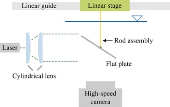
Experimental apparatus to visualize the flow field.

In this regard, we seek a simple theory to estimate the forces that enable insects to be airborne without resorting to empirical lift coefficients. We construct a scaling law for the lift of hovering insects as a function of their morphological and kinematic parameters. The simple physical understanding obtained through this work can help one to elucidate the evolutionary pressure of shape and kinematics of insect wings, and to establish design rules for flapping-based micro air vehicles.
We first revisit conventional aerodynamics to check its relevance. In the conventional steady potential-flow theory, the lift of a wing is obtained by the following two steps. First, the flow field around the wing is determined by the continuity equation and the boundary conditions composed of a kinematic boundary condition on the wing surface, a smooth flow-off requirement at the trailing edge and the far-field velocity. These kinematic relations give the velocity field and instantaneous circulation around the wing. Second, the Kutta–Joukowski theorem gives the lift of the wing as the product of the fluid density, the free-stream velocity and the circulation bound to the wing (Newman Reference Newman1977). We suppose that the first kinematic step still holds for hovering insect wings because the separating flow is confined around the leading edge vortex and a smooth flow-off condition is recovered at the trailing edge (Birch & Dickinson Reference Birch and Dickinson2003; Sane Reference Sane2003). However, the second dynamic step is far from valid for hovering insect wings, which flap in a cyclic manner only after several chord lengths of travel. The separated vorticity of the leading and trailing edges remains in the vicinity of the wing during most of the stroke cycle (Poelma Reference Poelma, Dickson and Dickinson2006; Liu & Aono Reference Liu and Aono2009; Jardin et al. Reference Jardin, Farcy and David2012). Instead of the Kutta–Joukowski theorem, we need to consider the momentum of the flow field induced by the vortical structures around the wing directly so as to model the lift.
In the following, therefore, we first approximate the instantaneous circulation of the leading edge vortex of hovering wings, which is assumed to play a dominant role in lift production, using the steady theory. We next measure the strength of the leading edge vortex of a dynamically scaled robot wing to test whether the steady aerodynamic theory provides a reasonable approximation for the strength of the leading edge vortex. We then construct a novel model for the momentum induced by the vortical structure around the wing, which eventually determines the lift. Our theory is tested by comparing the scaling law with the weight data for various species of insects.
2. Experimental apparatus
A rectangular rigid acrylic flat plate of 1 mm thickness is attached to a rod, which is driven by a linear stage (Newport IMS-LM), as shown in figure 1. The span of the plate is varied as 4, 6 and 8 cm and its chord is varied as 1.5, 2, 2.5, 3.5 and 4 cm. The flat plate and rod assembly is immersed in a water tank measuring 125, 15 and 25 cm in length, width and depth respectively. The free surface is 10 cm above the top of the flat plate. While the plate is linearly translated along the length of the water tank, the velocity varies sinusoidally to complete a half-period as
 $U(t)=U_{0}\sin ({\rm\pi}t/T)$
for the time interval
 $0<t<T$
, with
 $U_{0}$
being the maximum velocity. The velocity fields and vorticity contours are obtained by two-dimensional DPIV. Polyamide particles of
 $50~{\rm\mu}\text{m}$
diameter are used as seeding particles. The central plane perpendicular to the plate is illuminated to visualize seeding particles with an 8 W continuous laser of 532 nm wavelength through a slit. The images captured by a high-speed camera (Photron APX-RS), consisting of
 $1024\times 1024$
pixels, are analysed to generate a velocity field with a
 $64\times 64$
interrogation size and a 75 % overlap. The derived velocity vectors are validated by a dynamic mean value operator. The vorticity field is obtained using commercial graphic software based on the derived velocity field.
3. Results and discussion
3.1. Estimation of leading edge vortex strength
The shear flow separated at the leading edge of a hovering insect wing spirals into the leading edge vortex. Thus, the strength of the leading edge vortex is related to that of the shear flow generated on the wing, which is modelled as vortex sheets in the classical steady aerofoil theory. We scale the strength of the leading edge vortex via the circulation around a three-dimensional wing (Newman Reference Newman1977),
 ${\it\Gamma}$
, as
 $$\begin{eqnarray}{\it\Gamma}\sim \frac{U\overline{c}{\it\Lambda}\sin {\it\alpha}}{{\it\Lambda}+2},\end{eqnarray}$$
where
 ${\sim}$
signifies ‘is scaled as’,
 $U$
is the free-stream velocity,
 ${\it\alpha}$
is the angle of attack and
 $\overline{c}$
is the mean chord. Here,
 ${\it\Lambda}=R/\overline{c}$
is the aspect ratio, with
 $R$
being the wing span. To test whether the present model provides a reasonable approximation for the strength of the leading edge vortex on wings operated in hovering conditions, we measured the vorticity of flows around a flat plate translating linearly at high angles of attack within a water tank. The ranges of all independent parameters, such as wing velocity, stroke distance, angle of attack, wing span and chord, were selected to dynamically scale the characteristic values of the wings of hovering insects (see the supplementary data available at http://dx.doi.org/10.1017/jfm.2015.568). The Reynolds number,
 $\mathit{Re}={\it\rho}U\overline{c}/{\it\mu}$
, ranged from 200 to 3500, the dimensionless stroke amplitude (
 $A$
, the ratio of stroke distance to mean chord) from 1.6 to 3.4,
 ${\it\alpha}$
from
 $25^{\circ }$
to
 $70^{\circ }$
and
 ${\it\Lambda}$
from 1.5 to 2.7.
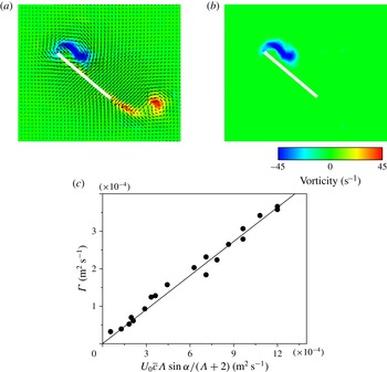
Figure 2(a) displays the representative velocity field and the resulting vorticity contours. The leading edge vortex was identified using the criteria proposed by Jeong & Husssain (Reference Jeong and Hussain1995), as shown in figure 2(b). Figure 2(c) plots the measured instantaneous circulation in the leading edge vortex at
 $t=T/2$
during translation according to the scaling law (3.1) for 19 cases. All of the data collapse onto a straight line with a slope 3.06, which is very close to the value expected from conventional aerodynamics,
 ${\rm\pi}$
(Newman Reference Newman1977).
(a) Velocity field and vorticity contour around a translating wing with
 $\mathit{Re}=2500$
,
 ${\it\alpha}=45$
,
 $A=1.7$
at
 $t=T/2$
. (b) Isolated leading edge vortex around an identical wing. (c) Instantaneous circulation,
 ${\it\Gamma}$
, of the leading edge vortex at
 $t=T/2$
versus the scaling parameter
 $U_{0}\overline{c}{\it\Lambda}\sin {\it\alpha}/({\it\Lambda}+2)$
.

3.2. A model for lift
Now we move on to the lift of hovering insects by considering the momentum induced by the vortical structure generated by the wing stroke. Because the vortical structure around the wing is characterized as the vortex loop over the wing (Poelma Reference Poelma, Dickson and Dickinson2006; Liu & Aono Reference Liu and Aono2009; Jardin et al.
Reference Jardin, Farcy and David2012), we approximate the momentum induced by the vortical structure,
 ${\rm\Delta}I$
, as
 ${\rm\Delta}I\sim {\it\rho}{\it\Gamma}S\sim {\it\rho}{\it\Gamma}R\overline{c}$
(Dickinson Reference Dickinson1996; Wu et al.
Reference Wu, Ma and Zhou2006; Lee et al.
Reference Lee, Park, Jeong, Cho and Kim2013). The reaction force exerted on the wing due to the time derivate of vortical impulse is scaled as
 $F\sim {\rm\Delta}I/T\sim {\it\rho}{\it\Gamma}R\overline{c}/T$
, which is perpendicular to the wing surface. Here,
 $T$
is the flapping period.
For the flapping translation of hovering insects, the linear velocity of the wing is scaled as
 $U\sim {\it\Phi}Rn$
, with
 ${\it\Phi}$
and
 $n$
being the stroke amplitude and flapping frequency respectively. Thus, the circulation around the leading edge vortex can be scaled as
 ${\it\Gamma}\sim {\it\Phi}Rn\overline{c}{\it\Lambda}\sin {\it\alpha}/({\it\Lambda}+2)$
via the scaling relation (3.1). By combining these relations, we obtain the scaling approximations of lift and drag with respect to the stroke plane as
 $L\sim {\it\rho}{\it\Phi}R^{2}\overline{c}^{2}n^{2}{\it\Lambda}\sin {\it\alpha}\cos {\it\alpha}/({\it\Lambda}+2)$
and
 $D\sim {\it\rho}{\it\Phi}R^{2}\overline{c}^{2}n^{2}{\it\Lambda}\sin ^{2}{\it\alpha}/({\it\Lambda}+2)$
respectively. The vertical component of the aerodynamic force produced balances the insect weight,
 $W$
. The contribution of drag to the vertical component of the period-averaged aerodynamic force is very small compared with that of lift because the drags during up- and downstrokes cancel each other out except for dragonfly-like wing motions having severe asymmetry of up- and downstrokes (Wang Reference Wang2004; Park & Choi Reference Park and Choi2012). By balancing the vertical component of the lift with the insect weight, we obtain
 $$\begin{eqnarray}W\sim 0.5{\it\rho}{\it\Phi}R^{2}\overline{c}^{2}n^{2}\frac{{\it\Lambda}\sin 2{\it\alpha}}{{\it\Lambda}+2}\cos {\it\beta},\end{eqnarray}$$
where
 ${\it\beta}$
is the stroke plane angle, that is, the angle between the horizontal and stroke planes. We note that our scaling law for the lift is consistent with the novel dimensionless thrust proposed by Dewey et al. (Reference Dewey, Boschitsch, Moored, Stone and Smits2013),
 $L\sim {\it\rho}R^{2}c^{2}n^{2}{\it\eta}$
, where
 ${\it\eta}$
is a function of geometrical parameters, as mentioned in § 1.
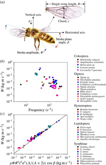
(a) Illustration to define morphological and kinematical parameters of hovering insects. (b,c) Weight of the insect versus (b) frequency and (c) the scaling parameter
 ${\it\rho}{\it\Phi}R^{2}\overline{c}^{2}n^{2}({\it\Lambda}/({\it\Lambda}+2))\cos {\it\beta}$
. We compare our theory with experimental observations (83 data points) for 35 species of hovering insects (Weis-Fogh Reference Weis-Fogh1973; Ellington Reference Ellington1984c
,Reference Ellington
d
; Ennos Reference Ennos1989; Willmott & Ellington Reference Willmott and Ellington1997a
,Reference Willmott and Ellington
b
; Fry et al.
Reference Fry, Sayaman and Dickinson2005; Liu & Sun Reference Liu and Sun2008; Walker et al.
Reference Walker, Thomas and Taylor2010; Mou, Liu & Sun Reference Mou, Liu and Sun2011). In (c), the straight line corresponds to
 $y=11.4x$
.

We first compare our theory for lift with the data (see the supplementary data) for 35 species of hovering insects from previously published papers that report the wing dimensions, flapping frequency and body weight (Weis-Fogh Reference Weis-Fogh1973; Ellington Reference Ellington1984c
,Reference Ellington
d
; Ennos Reference Ennos1989; Willmott & Ellington Reference Willmott and Ellington1997a
,Reference Willmott and Ellington
b
; Fry et al.
Reference Fry, Sayaman and Dickinson2005; Liu & Sun Reference Liu and Sun2008; Walker et al.
Reference Walker, Thomas and Taylor2010; Mou et al.
Reference Mou, Liu and Sun2011). While the raw data scatter considerably when plotted against one of the most influential factors in the force production, the flapping frequency, figure 3(b), the data plotted according to the scaling law collapse onto a master curve, figure 3(c). Since most of the experimental observations do not report the angle of attack, we have simply modified the scaling law by ignoring
 $\sin 2{\it\alpha}$
. Considering that the right-hand side of equation (3.2) varies by up to six orders of magnitude without
 $\sin 2{\it\alpha}$
, the variation of
 $\sin 2{\it\alpha}$
for different insects is indeed insignificant. It varies from 0.6 to 0.9 with the angle of attack changing from
 $20^{\circ }$
to
 $60^{\circ }$
. We validate our theory further with the data for six species of insects for which the angle of attack during each half-stroke is known (Ellington Reference Ellington1984c
,Reference Ellington
d
; Willmott & Ellington Reference Willmott and Ellington1997a
,Reference Willmott and Ellington
b
; Fry et al.
Reference Fry, Sayaman and Dickinson2005; Liu & Sun Reference Liu and Sun2008; Walker et al.
Reference Walker, Thomas and Taylor2010; Mou et al.
Reference Mou, Liu and Sun2011). The weight of the insect normalized by the dynamic pressure force,
 $0.5{\it\rho}U^{2}R\overline{c}$
, with the characteristic wing tip velocity
 $U\sim {\it\Phi}Rn$
and the wing area
 $R\overline{c}$
, is scaled as
 $$\begin{eqnarray}\frac{2W}{{\it\rho}R^{3}{\it\Phi}^{2}\overline{c}n^{2}}\sim \frac{\overline{c}}{R{\it\Phi}}\frac{{\it\Lambda}}{{\it\Lambda}+2}\cos {\it\beta}\sin 2{\it\alpha}.\end{eqnarray}$$
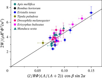
We plot the experimental data according to the dimensionless scaling law (3.3) in figure 4. The scaling law agrees favourably with the experimental observations, with the slope of the best-fitting straight line being 46.2.
Experimental validation of the normalized scaling law, (3.3). We compare our theory with experimental observations (32 data points) for six species of hovering insects (Ellington Reference Ellington1984c ,Reference Ellington d ; Willmott & Ellington Reference Willmott and Ellington1997a ,Reference Willmott and Ellington b ; Fry et al. Reference Fry, Sayaman and Dickinson2005; Liu & Sun Reference Liu and Sun2008; Walker et al. Reference Walker, Thomas and Taylor2010; Mou et al. Reference Mou, Liu and Sun2011).

Our analysis is distinguished from the conventional steady potential-flow theory in that the lift is scaled as
 $L\sim {\it\rho}{\it\Gamma}\overline{c}R/T$
rather than
 $L\sim {\it\rho}{\it\Gamma}UR$
, with
 $U\sim {\it\Phi}Rn$
(see appendix A). This is mainly due to the difference in the vorticity generation process. The steady lift production arises from the formation of trailing vortices at wing tips (freely convecting chordwise vorticity), with its generation rate proportional to the translational velocity
 $U$
while the spanwise vortex sheet is bound to the wing surface. As a result, the evolution of the vortical structure around the steady wing can be modelled by a single vortex loop with a monotonically increasing area (Newman Reference Newman1977; Dickinson Reference Dickinson1996; Wu et al.
Reference Wu, Ma and Zhou2006). In contrast, on a hovering insect wing, the vorticity is generated all around the edges, including the spanwise vorticity at the leading edge (Poelma Reference Poelma, Dickson and Dickinson2006; Liu & Aono Reference Liu and Aono2009). We have shown that it is the generation of spanwise vorticity along the wing edges that plays a crucial role in producing lift for hovering insects. We also compare our theory and conventional theory with the lift measurement data for reciprocally translating wings given by Lentink & Dickinson (Reference Lentink and Dickinson2009) in appendix B.
4. Conclusions
Our theory has been shown to successfully capture the dominant physical mechanism underlying the lift generation in hovering flight, allowing us to obtain a simple scaling law for the lift with given morphological and kinematic parameters of the insects. However, detailed fluid-dynamic phenomena associated with hovering, such as time-dependent flow structures, the force history and the interaction with the wake, can be adequately accounted for by numerically computing the full Navier–Stokes equation.
We believe that our theory will not only help one to grasp the essential aerodynamics of hovering easily but also shed light on some biological observations that have eluded scientific explanation based on conventional theory for decades (Ellington Reference Ellington1984a
; Dickinson et al.
Reference Dickinson, Lehmann and Sane1999). For instance, the wing load,
 $W/(R\overline{c})$
, of the hoverfly Syrphus balteatus is
 ${\sim}8.97~\text{N}~\text{m}^{-2}$
, which is similar to that of the crane fly Tipula paludosa (
 ${\sim}9.11~\text{N}~\text{m}^{-2}$
) despite dramatic differences in their wing size and kinematics (see the supplementary data). The stroke angle of the hoverfly wing ranges only from
 $60^{\circ }$
to
 $70^{\circ }$
, which is almost half of the typical stroke angle of many hovering insects including the crane fly. The wing chords of the two insects are similar (2.98 mm for the hoverfly and 3.09 mm for the crane fly), but the wingspan of the hoverfly, approximately 9.9 mm, is almost half that of the crane fly. However, the flapping frequency of the hoverfly (124 Hz), which is almost twice as high as that of the crane fly (58 Hz), successfully compensates for such disadvantages. Our theory allows us to explain this observation because
 $W/(R\overline{c})$
is proportional to
 $n^{2}$
, but scales linearly with
 $R$
and
 ${\it\Phi}$
:
 $W/(R\overline{c})\sim n^{2}R{\it\Phi}$
. In other words, hoverflies flap their wings just fast enough to surmount the drawbacks of small stroke angle and wingspan. The conventional theory cannot account for this morphological and kinematic dependence because it predicts
 $W/(R\overline{c})\sim n^{2}R^{2}{\it\Phi}^{2}$
. Our theory provides a clear fluid-dynamic explanation of how different evolutionary selections for wing kinematics and morphology among insect species can arrive at the same functionality: hovering with similar wing loads. We also expect that our scaling law will be a simple yet powerful guideline for designing flapping-based micro air vehicles.
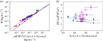
Experimentally measured weight of hovering insects plotted according to (a) scaling law (A 1) and (b) normalized scaling law (A 2) based on the conventional steady potential-flow theory. In (a), the black and red lines correspond to
 $y\sim x$
and
 $y\sim x^{0.87}$
respectively. The symbols are from figure 3.

Acknowledgements
This work was supported by the National Research Foundation of Korea (Grant nos. 2011-0028032, 2014048162 and 2014023206) via SNU IAMD.
Supplementary data
Supplementary data is available at http://dx.doi.org/10.1017/jfm.2015.568.
Appendix A. Scaling law based on the conventional steady potential-flow theory
In the conventional steady potential-flow theory, the lift and circulation of the leading edge vortex can be written as
 $L\sim {\it\rho}{\it\Gamma}UR$
and
 ${\it\Gamma}\sim U\overline{c}{\it\Lambda}\sin {\it\alpha}/({\it\Lambda}+2)$
respectively (Newman Reference Newman1977; Dickinson Reference Dickinson1996). Since the flapping velocity
 $U\sim {\it\Phi}Rn$
, the vertical force that balances the weight is scaled as
 $$\begin{eqnarray}W\sim {\it\rho}{\it\Phi}^{2}R^{3}\overline{c}n^{2}\frac{{\it\Lambda}}{{\it\Lambda}+2}\sin {\it\alpha}\cos {\it\beta}.\end{eqnarray}$$
The normalized form is given by
 $$\begin{eqnarray}\frac{W}{{\it\rho}R^{3}{\it\Phi}^{2}\overline{c}n^{2}}\sim \frac{{\it\Lambda}}{{\it\Lambda}+2}\sin {\it\alpha}\cos {\it\beta}.\end{eqnarray}$$
We first plot the experimental data according to (A 1) in figure 5(a). The data appear to collapse onto a master curve with the conventional theory for an obvious reason that the pressure forces exerted on the wing would grow with the dynamic pressure and the surface area. However, investigation of the slopes of the lines reveals a significant difference between the plots using conventional theory (figure 5
a) and our theory (figure 3
c). For the conventional theory to hold, the data should collapse onto a line representing
 $y=ax$
in log–log plot, where
 $y$
and
 $x$
represent the values of the vertical and horizontal axes respectively. This is shown as a black line in the figure. Obviously, the biological data do not follow the line
 $y\sim x$
. Rather, the least-square method finds the best-fitting line for the biological data to be
 $y\sim x^{0.87}$
, the red line. This implies that the biological data are consistent with the following power law:
 $W\sim \left[{\it\rho}{\it\Phi}^{2}R^{3}\bar{c}^{2}n^{2}\cos {\it\beta}{\it\Lambda}/({\it\Lambda}+2)\right]^{0.87}$
, which has no theoretical background. We further plot the experimental data according to the normalized scaling law (A 2) in figure 5(b). The data are scattered rather than collapsing onto a single master curve as in figure 4.
Appendix B. Comparison with previous experiments on flapping locomotion
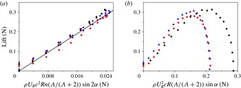
We compare our theory and the conventional model with the lift measurement data for reciprocally translating wings given by Lentink & Dickinson (Reference Lentink and Dickinson2009), as shown in figure 6. The lift increases linearly with our scaling law, figure 6(a), whereas the lift does not follow what the conventional theory predicts, figure 6(b). In more detail, the experimental data for
 $\mathit{Re}=110$
(circles) and 1400 (triangles) were collected with the same velocity but by varying the density and viscosity of the fluid. For
 $\mathit{Re}=14\,000$
(squares), the velocity of the wing and the physical properties of the fluid were altogether changed compared with the cases of
 $\mathit{Re}=1400$
and 110. The data plotted according to the conventional model show significant inconsistency when the wing velocity is changed, whereas all of the data collapse onto a single line when plotted according to our scaling law.
The experimentally measured lift of the reciprocally translating wing in Lentink & Dickinson (Reference Lentink and Dickinson2009) plotted according to (a) our scaling law and (b) the conventional steady potential-flow theory. The circles, triangles and squares correspond to
 $\mathit{Re}=110$
, 1400 and 14 000.