




1. Introduction
The decaying homogeneous isotropic turbulence (DHIT) in a periodic domain is the simplest form of turbulent flow. Although this kind of flow only approximately exists in nature and industrial applications, it provided opportunities to understand the complexity of turbulence. How the turbulent kinetic energy (TKE) decays with time is one of the basic questions in DHIT. The theoretical studies on this topic started from the classic work of Kolmogorov (Reference Kolmogorov1941), who argued that the decay of TKE in DHIT should be independent of the viscosity and followed a power law  $E(t)/E(t_0) \propto t^{-n}$, where
 $E(t)$ and
 $E(t_0)$ are the current and initial volume-averaged TKE, respectively. Kolmogorov also derived the analytical exponent
 $n = 10/7$ for large-Reynolds-number isotropic turbulence (Kolmogorov Reference Kolmogorov1941). Batchelor (Reference Batchelor1948) provided a more complete analysis of the decay rate with different assumptions. In the same work, he pointed out that exponent
 $n$ would change from
 $10/7$ to
 $5/2$ when DHIT reached its final stage. However, Saffman (Reference Saffman1967) argued that the prerequisite leading to
 $n = 10/7$ so that the ‘Loitsianskii integral’ remained constant in the decay process could not generally hold, so
 $n = 6/5$ was to be expected. In the literature, the former type of turbulence following the
 $10/7$ decay rate is usually termed the Batchelor turbulence, while the latter one obeying the
 $6/5$ law is the Saffman turbulence. Under the limiting case of infinite Reynolds number,
 $n = 1$ was derived by George (Reference George1992) as the exponent of power-law decay at the asymptotic state (George Reference George1992). Lin (Reference Lin1948) also reached a similar conclusion and showed good agreement between the theory and those early experimental results.
Other than the theoretical studies, experiments and numerical simulations were also conducted to calibrate the decay rate of TKE in DHIT. With a few exceptions observing a log-law decay of TKE (Hurst & Vassilicos Reference Hurst and Vassilicos2007; Seoud & Vassilicos Reference Seoud and Vassilicos2007; George & Wang Reference George and Wang2009), most studies confirmed that fully developed turbulence would follow power-law decay. However, as reviewed by Yoffe & McComb (Reference Yoffe and McComb2018), the exponent  $n$ reported in the literature varies. The pioneering experiments of Comte-Bellot & Corrsin (Reference Comte-Bellot and Corrsin1966, Reference Comte-Bellot and Corrsin1971) with grid turbulence found that the decay exponent
 $n$ ranged between 1.16 and 1.37. Similar exponents were reported in other grid-turbulence experiments, to name a few:
 $n \approx 1.3$ by Mohamed & Larue (Reference Mohamed and Larue1990);
 $n = 1.13\pm 0.02$ by Krogstad & Davidson (Reference Krogstad and Davidson2010); and
 $n = 1.18\pm 0.02$ by Sinhuber, Bodenschatz & Bewley (Reference Sinhuber, Bodenschatz and Bewley2015). Unlike experimental studies, simulations can easily generate both Batchelor and Saffman types of turbulence by prescribing different initial forms of energy spectra (Huang & Leonard Reference Huang and Leonard1994; Mansour & Wray Reference Mansour and Wray1994; Yu, Girimaji & Luo Reference Yu, Girimaji and Luo2005; Anas, Joshi & Verma Reference Anas, Joshi and Verma2020). However, due to the limitation of computational resources, most simulations are restricted to relatively low Reynolds numbers. At small Reynolds numbers,
 $n$ generally decreased with the Reynolds numbers (Huang & Leonard Reference Huang and Leonard1994; Mansour & Wray Reference Mansour and Wray1994; Djenidi, Kamruzzaman & Antonia Reference Djenidi, Kamruzzaman and Antonia2015).
When a dispersed phase is present in the carrier turbulence, it can significantly modify the properties of turbulence. Such effects are called turbulence modulation. Over the years, turbulence modulation has been extensively studied in different types of turbulent flows. Specifically, particular attention was paid to whether particles would augment or attenuate the intensity of turbulence. Due to its relative simplicity of DHIT, turbulence modulation in DHIT was also extensively studied. Elghobashi & Truesdell (Reference Elghobashi and Truesdell1993) conducted numerical simulations to investigate the interaction between decaying turbulence and inertial particles and reported that a faster decay rate of TKE could be observed with particles when the effect of gravity was absent. When particles follow the Stokes drag,  $(\boldsymbol {v} - \boldsymbol {u})/\tau _p$ would appear in the fluid momentum equation, where
 $\boldsymbol {v}$ and
 $\boldsymbol {u}$ are the velocity of the fluid and particle phases, respectively, and
 $\tau _p$ is the particle response time. As a result, the presence of particles induces an extra term
 $(\langle \boldsymbol {u}'\boldsymbol{\cdot}\boldsymbol {v}'\rangle - \langle \boldsymbol {u}'\boldsymbol{\cdot}\boldsymbol {u}'\rangle )/\tau _p$ in the TKE budget equation, where
 $\langle \cdots \rangle$ means the ensemble averaging. Since the self-correlation
 $\langle \boldsymbol {u}'\boldsymbol{\cdot}\boldsymbol {u}'\rangle$ is usually greater than the cross-correlation
 $\langle \boldsymbol {u}'\boldsymbol{\cdot}\boldsymbol {v}'\rangle$ when
 $\vert \boldsymbol {u}'\vert$ and
 $\vert \boldsymbol {v}'\vert$ are of the same order, this extra term is expected to be negative and acts as an additional dissipation rate. However, Ferrante & Elghobashi (Reference Ferrante and Elghobashi2003) described an opposite scenario where heavy tracer particles reduced the decay rate of the TKE in DHIT. Unlike inertial particles, these heavy tracer particles do not increase viscous dissipation, but their large density could significantly enhance the system inertia and resist the TKE decay. By summarizing the results of turbulence modulation in the literature, Elgobashi (Reference Elgobashi2006) generated a classification map of turbulence modulation based on the ratio between particle response time and Kolmogorov time
 $\tau _k$, i.e. the Stokes number. This map suggested that the decay rate of TKE would be enhanced by particles when
 $\tau _{p}/\tau _{k} \geq 1$ and reduced when
 $\tau _{p}/\tau _{k} \leq 0.1$. Particles with intermediate
 $\tau _p/\tau _k$ behaved like ghost particles, causing insignificant modulation to TKE. Abdelsamie & Lee (Reference Abdelsamie and Lee2012) also observed an increased decay rate of TKE in DHIT when particles have
 $\tau _{p}/\tau _{k} \geq 1$.
Turbulence modulation can be far more complex when the sizes of the dispersed particles are comparable or greater than the Kolgomorov length, i.e. finite-size particles. Such complexity is mainly due to the significant distortion and discontinuity brought by the particles to the fluid phase, which makes it challenging to model the disturbed flow around particles (Eaton Reference Eaton2009). Burton & Eaton (Reference Burton and Eaton2005) contrasted the TKE and dissipation rate around a fixed particle in a DHIT with the unladen case. They observed significantly enhanced local dissipation in the region within 1.5 diameters from the particle surface, which described the turbulence modulation as a local effect. Lucci, Ferrante & Elghobashi (Reference Lucci, Ferrante and Elghobashi2010) simulated the two-way coupling effect between particles with sizes around the Taylor microscale and DHIT. Although particles generated additional TKE through the two-way coupling effect, it was insufficient to compensate for the locally enhanced dissipation rate, which eventually resulted in a faster decay rate of TKE than the unladen case. Similar observations were made by Schneiders, Meinke & Schröder (Reference Schneiders, Meinke and Schröder2017), who used accurate numerical simulations to study the effect of Kolmogorov-scale particles with particle-to-fluid density ratio ranging from 40 to 5000 on a DHIT and found that the decay rate of TKE in particle-laden flows was always faster with particles. In contrast, Luo et al. (Reference Luo, Wang, Li, Tan and Fan2017) studied the modulation of DHIT by heavy particles but found that heavy particles slowed down the decay rate of TKE. These opposite observations of Schneiders et al. (Reference Schneiders, Meinke and Schröder2017) and Luo et al. (Reference Luo, Wang, Li, Tan and Fan2017) are possibly due to the different particle sizes in the two studies, which are larger in the latter.
These above studies covered how particles modified the decay rate of TKE in DHIT. However, we noted that most of them focused on the early stage of the decay, where the particle-turbulence system is not fully relaxed. Since the power-law decay requires the flow to evolve until a specific form of the energy spectrum is established, the lack of data in the late stage brings uncertainty about whether particle-laden DHIT still follows a power law. In a few studies focusing on validating simulation methods, power-law decay of TKE in particle-laden DHIT was shown, but whether this observation is generalizable requires some further investigation (Brändle de Motta et al. Reference Brändle de Motta2019; Peng et al. Reference Peng, Ayala, Brändle de Motta and Wang2019). How the exponent of the power-law decay changes with the flow and particle parameters still needs to be answered.
Another piece of information missing in the literature is the lack of criteria to predict under what conditions a fully relaxed particle-laden DHIT would decay faster or slower than the unladen single-phase case. For other types of turbulent flows, such as turbulent jets and wall-bounded turbulence, predictive criteria depending on the flow and particle parameters are available to identify the threshold when the turbulence modulation transits from augmentation to attenuation (Gore & Crowe Reference Gore and Crowe1989; Righetti & Romano Reference Righetti and Romano2004; Tanaka & Eaton Reference Tanaka and Eaton2008; Yu et al. Reference Yu, Xia, Guo and Lin2021). Compared with other types of turbulence, modelling the turbulence modulation in HIT could contribute more to the development of multiphase large-eddy simulation (LES) or Reynolds-averaged Navier–Stokes (RANS) simulation since the subgrid turbulence is usually assumed to be isotropic. However, as mentioned earlier, the existing criterion that a faster decay is expected when  $\tau _p/\tau _k \ge 1$ applies better to the early stage, where the addition of particles introduces a sudden enhancement of local dissipation.
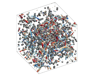
The present study conducts particle-resolved direct numerical simulation (PR-DNS) to investigate the turbulence modulation induced by monodispersed finite-size particles in HIT. Unlike the previous studies focusing on the early stage of decay, e.g. Lucci et al. (Reference Lucci, Ferrante and Elghobashi2010) and Gao, Li & Wang (Reference Gao, Li and Wang2013), this study pays more attention to the later times where a power-law decay is possibly established. Since the initial condition could significantly affect the power-law decay exponent, we configure particle-laden DHIT simulation with two different set-ups, i.e. releasing particles to a single-phase DHIT or turning off the large-scale forcing in a sustaining particle-laden HIT. Simulations with varying particle sizes, density ratios and volume fractions are conducted to investigate how particle parameters affect turbulence modulation. A model to predict the effect of particle presence on the decay exponent is also developed from the energy budget equation of the two-phase DHIT and validated by the simulation results.
The remainder of the paper is structured as follows. In § 2, we introduce the two set-ups to initialize particle-laden DHIT simulations and the associated parameter settings. The simulation details are also briefly covered. The main results of the simulations and the efforts to establish a model to predict how particles affect the decay rate of TKE in DHIT are discussed in § 3. Finally, we recapitulate the main conclusions in § 4.
2. Parameter setting and simulation details
The present study conducts PR-DNS to analyse how particles affect the decay rate of DHIT. The simulations are conducted using the lattice Boltzmann method, a second-order accurate flow solver that solves the Navier–Stokes equations indirectly in the higher dimensional phase space where the model Boltzmann equation is applied. This mesoscopic approach tracks the evolution of the particle distribution function. Here, the particles are the model fluid molecular particles travelling on designated straight lines; they are microscopic objects utterly different from the macroscopic finite-size solid particles.
The no-slip boundary conditions on the moving particle surfaces are treated with interpolated bounce-back schemes to ensure the velocity field preserves second-order accuracy. The short-range hydrodynamic interactions between nearby particles and particle collisions are handled with the lubrication force and the soft-sphere collision, respectively (Brändle de Motta et al. Reference Brändle de Motta, Breugem, Gazanion, Estivalezes, Vincent and Climent2013). For a detailed introduction to the simulation method and validations, readers can refer to Peng (Reference Peng2018). The capability of this method to simulate single-phase and particle-laden decaying HIT was also cross-examined with other methods developed by our collaborators, e.g. the finite-volume-based immersed boundary method and Lagrangian volume of fluid method by Brändle de Motta et al. (Reference Brändle de Motta2019), and our in-house lattice-Boltzmann method based immersed boundary method by Peng et al. (Reference Peng, Ayala, Brändle de Motta and Wang2019).
The background HIT is generated using the stochastic large-scale forcing scheme of Eswaran & Pope (Reference Eswaran and Pope1988). We recently used the same approach to generate sustainable HIT and study how particle and flow parameters affected the turbulence modulation (Peng, Sun & Wang Reference Peng, Sun and Wang2023). Since this approach was validated against an in-house pseudo-spectral code in our recent work (Peng et al. Reference Peng, Sun and Wang2023), we do not perform further validations of the numerical approach in the present study.
There are at least two ways to generate decaying particle-laden HIT. The first way is to create an unladen single-phase DHIT, then release particles at the initial state of the decay. Under this set-up, the primary turbulence modulation happens right after the addition of particles in the form of suddenly increased dissipation rates since the fluid flows need some time to relax due to the significant local disturbances induced by the presence of particles (Burton & Eaton Reference Burton and Eaton2005; Lucci et al. Reference Lucci, Ferrante and Elghobashi2010; Gao et al. Reference Gao, Li and Wang2013). The main advantage of this set-up is that for each particle-laden case, there is a well-defined corresponding single-phase case sharing the same starting point, which makes assessing the turbulence modulation contributed by particles easy. However, the suddenly enhanced dissipation rate decays quickly and may become invisible when the power-law decay starts. In most previous studies of particle-laden DHIT, the flow is initialized this way (Lucci et al. Reference Lucci, Ferrante and Elghobashi2010; Gao et al. Reference Gao, Li and Wang2013; Brändle de Motta et al. Reference Brändle de Motta2019). An alternative way to generate particle-laden DHIT is to first simulate sustainable HIT with the large-scale forcing until the statistical stationary state, then turn off the forcing so the fully relaxed particle-laden HIT would decay with time. Since the dispersed and carrier phases have already been sufficiently mixed, this set-up avoids sudden dissipation rate jumps at the initial stage. However, since the decay starts from an already disturbed particle-laden flow, the corresponding single-phase flow is no longer retrievable.
In the present study, we shall consider particle-laden DHIT generated in both ways. From the dimensional analysis, one can conclude that the turbulence modulation depends on four non-dimensional parameters: the flow Reynolds number  $Re_\lambda$, where
 $\lambda$ is the Taylor microscale, the particle-to-fluid density ratio
 $\rho = \rho _p/\rho _f$, the relative particle size
 $d_p/\eta$, where
 $\eta$ is the Kolmogorov length, and the volume fraction
 $\phi _p$. Note that, for simplicity, the sedimentation of particles due to the gravitational acceleration and its effects on the turbulence modulation are not considered in the current paper. Except for the flow Reynolds number
 $Re_\lambda$, the other three controlling non-dimensional parameters are varied, whose values are summarized in table 1. For the first set-up, we initialize the single-phase HIT with the velocity and pressure fields taken from a sustained HIT simulation at eight different moments. The time-averaged Reynolds number of this sustained HIT is
 $Re_\lambda = 74.15\pm 0.33$, and the actual
 $Re_\lambda$ when the flow starts to decay ranges from
 $73.08$ to
 $80.43$. With or without the addition of particles, the decaying flow would require some time for the power-law decay to be established. We also record the Reynolds number when the power-law decay begins, i.e.
 $Re_{\lambda,d}$. The values of
 $Re_{\lambda,d}$ with different initial conditions vary between
 $13.73$ and
 $33.13$.
Parameter settings of the single-phase and particle-laden DHIT simulations. Quantities from the second to the last column are the Reynolds number when the flow starts to decay, the Reynolds number at the starting point of the power-law decay stage, the particle-to-fluid density ratio, the ratio between particle diameter and the time-averaged Kolmogorov length of the single-phase sustained HIT simulation, and the particle volume fraction. Acronyms ‘SP’, ‘PL1’ and ‘PL2’ represent single-phase DHIT and particle-laden DHIT initialized with the first and second set-ups. A total number of 336 cases are simulated. For conciseness, the information for different cases is condensed as ranges. The specific values in each simulated case are provided in the Supplementary Materials available at https://doi.org/10.1017/jfm.2024.698.

To save computational resources, the initial conditions for the second set-up come directly from the fluid and particle information saved from our sustained particle-laden HIT simulations reported in Peng et al. (Reference Peng, Sun and Wang2023). The flow and particle parameters with this set-up are also compiled in table 1. Same as the first set-up, for each set of flow and particle parameters, we configure multiple realizations with initial conditions taken from different moments of the specific sustained particle-laden HIT simulation.
All simulations are conducted with the computational domain of  $512^3$. For the Reynolds number chosen in the present study, this
 $512^3$ mesh results in a grid resolution of
 $k_{max}\eta \ge 5.7$, sufficient to resolve the Kolmogorov eddies in the flow fields (see validations in Peng et al. Reference Peng, Sun and Wang2023). PR-DNS also requires sufficient grid resolutions to represent particles, i.e.
 $d_p/\Delta x$ should also be large enough. In our previous study (Peng et al. Reference Peng, Ayala, Brändle de Motta and Wang2019), we compared the simulation results from two grid resolutions,
 $d_p/\Delta x = 12$ and
 $d_p/\Delta x = 24$ for a similar decaying particle-laden HIT but with a higher initial Reynolds number
 $Re_{\lambda,0} = 87.6$. Although the resolution of
 $d_p/\Delta x = 12$ was not able to obtain very accurate results of local TKE and dissipation rate distribution in the close vicinity of particle surfaces, it was sufficiently accurate to capture the temporal evolution of the averaged TKE, which is the essential quantity for the present study. In the present study,
 $d_p/\Delta x$ ranges from
 $16$ to
 $40$. Based on our previous grid convergence investigation, a resolution of
 $d_p/\Delta x = 16$ should be sufficient for the main objective of the present study.
3. Results and discussions
3.1. Decay rates of TKE in single-phase DHIT
Before analysing the decay rate in particle-laden HIT, we quantify the corresponding decay rate in the unladen single-phase cases for later comparisons. As mentioned in the last section, with the first set-up, we start the decaying flows from eight different time frames in a sustainable HIT simulation. The interval between arbitrary two consecutive frames exceeds  $20$ eddy turnover times to ensure sample independence of each realization. For the second set-up, there is no corresponding unladen DHIT for each specific particle-laden case since the flow has already been entirely disturbed. However, we may still create unladen DHIT cases with similar large-scale forcing for the purpose of comparison. Like the first set-up, these unladen DHIT cases are initialized with flow fields taken at different time frames of a sustainable HIT simulation. Sufficient time intervals are also kept between those time frames to ensure mutual independence among various realizations.
Figure 1 shows the temporal evolution of the normalized TKE,  $E/E_0$, in some selective single-phase DHIT, where
 $E_0 = 3u_0'^2/2$ denotes the value of the initial TKE and
 $u_0'$ is the initial root-mean-square velocity. After the driving force is turned off, the flow still takes some time to get rid of the memory effects of the large-scale forcing and reaches a fully developed stage where the power-law decay is established. To quantify the exponent
 $n$ more accurately, it is important to determine the beginning point of the power-law decay. As shown in figure 1, the power-law decay starts around
 $(t-t_0)/\tau _0 = 3$ for different initial Reynolds numbers, where
 $\tau _0 = {u_0^{\prime }}^2/\epsilon _0$ is the initial large eddy turnover time,
 $\epsilon _0$ represents the initial dissipation rate. Other than visually identifying the starting point of power-law decay, the Taylor microscale
 $\lambda \propto t^{1/2}$ is another commonly used criterion (George Reference George2013). This criterion validates since a power-law decaying TKE
 $E(t) = E_0 t^{-n}$ would result in
 \begin{equation} \frac{{\rm d} E}{{\rm d} t} ={-}n E_0 t^{{-}n-1} ={-}n\frac{E}{t} ={-}\epsilon ={-}\frac{10\nu E}{\lambda^{2}}, \end{equation}
where  $\nu$ is the kinematic viscosity, which leads to
 $\lambda \propto t^{1/2}$ for arbitrary exponent
 $n$. We also choose the
 $\lambda \propto t^{1/2}$ criterion to identify the starting point of the power-law decay.
Decay of the fluid TKE in single-phase DHIT with various initial  $Re_\lambda$. The time is normalized by the initial large eddy turnover time
 $\tau _0 ={u_0^{\prime }}^2/\epsilon _0$, where
 $u_0'$ and
 $\epsilon _0$ are the root-mean-square velocity and dissipation rate at the initial time
 $t_0$, respectively. The black vertical dashed line at
 $t - t_0 = 3\tau _0$ shows roughly the starting point of the power-law decay.

The temporal evolution of  $\lambda$ normalized by its initial value, i.e.
 $\lambda /\lambda _{0}$, in the single-phase cases is shown in figure 2 for some representative cases. The green dash-dotted line is a reference line for
 $\lambda \propto t^{1/2}$. For cases with both set-ups, the power-law decay starts roughly from
 $t - t_0 = 4\tau _0$. We used the least squares to fit the data points after
 $t - t_0 = 4\tau _0$ onto a straight line of
 $\lambda \propto t^{1/2}$ and obtained the
 $R^2$ value no less than
 $0.98$ in all cases. Other than the criterion mentioned above, some references, e.g. Huang & Leonard (Reference Huang and Leonard1994) and Djenidi et al. (Reference Djenidi, Kamruzzaman and Antonia2015), identify the power-law decay stage when the changing rate of the Taylor Reynolds number,
 $Re_\lambda$, becomes small. We also show
 $Re_\lambda /Re_{\lambda 0}$ of the representative cases in figure 3 and compute the relative change of
 $Re_\lambda$ after
 $t - t_0 = 4\tau _0$. It is confirmed that
 $\Delta Re_\lambda /Re_{\lambda 0}$ is less than 10 % for all cases, where
 $\Delta Re_\lambda$ is the change of
 $Re_\lambda$ from
 $t - t_0 = 4\tau _0$ to the end of the simulation, which is approximately
 $t_0+8\tau _0$. Based on this evidence, we believe using
 $t - t_0 = 4\tau _0$ as the starting time of the power-law decay is appropriate for the present study. The same criteria are used to determine the starting points of power-law decay in the particle-laden cases.
Temporal development of Taylor microscale  $\lambda$ normalized by its initial value,
 $\lambda /\lambda _{0}$, of single-phase flow for several selected cases with different
 $Re_\lambda$. Here,
 $\lambda _{0}$ denotes the value of Taylor microscale at
 $t = 0$. The black vertical dotted line indicates the time,
 $t - t_0 = 4\tau _0$, after which the power-law decay is established.

Taylor Reynolds number  $Re_\lambda$ of single-phase flow for several sets of cases with different
 $Re_\lambda$ in both set-ups.

After determining the starting points, the power-law decay exponent  $n_{sp}$ for the single-phase DHIT can be quantified from the numerical results using the least square fitting. To enhance the accessibility of the data, we compile those data in table 2 for the simulated single-phase DHIT. Most of the exponents fall between
 $1.5$ and
 $1.8$, which is higher than the counterparts observed in the experiments of grid turbulence, as summarized by Yoffe & McComb (Reference Yoffe and McComb2018). However, such deviation could be mainly because the Reynolds numbers in our simulations are relatively small. It is well known that the decay exponent strongly depends on
 $Re_{\lambda }$ and increases as the turbulence weakens, e.g. from
 $10/7$ to
 $5/2$ as analysed by Batchelor (Reference Batchelor1948). In a range of Reynolds number
 $Re_{\lambda,0}$ between 25.8 and 51.6, Yoffe & McComb (Reference Yoffe and McComb2018) observed
 $1.55\le n \le 1.61$ in their direct numerical simulations, which is similar to the values we obtained. It is also notable from table 2 that for similar Reynolds numbers,
 $n$ can vary significantly with the specific realizations used for the flow initialization.
Reynolds number and power-law decay exponent of single-phase DHIT.

3.2. Decay rates of TKE in particle-laden DHIT
We now move to the particle-laden cases. Figure 4 shows the temporal variation TKE in our particle-laden DHIT simulations, together with the data acquired from some previous studies (Lucci et al. Reference Lucci, Ferrante and Elghobashi2010; Luo et al. Reference Luo, Wang, Li, Tan and Fan2017; Schneiders et al. Reference Schneiders, Meinke and Schröder2017). All those previous studies generated particle-laden DHIT with the first set-up. Although these previous studies only had data points in limited time intervals as they mainly focused on studying the turbulence modulation at the initial decay stage, we can still observe that power-law decay starts to be established. One should note that the results of Luo et al. (Reference Luo, Wang, Li, Tan and Fan2017) have been rescaled in figure 4 since this work may have used a different definition of  $\tau _0$, i.e.
 $0.5u_0'^2/\epsilon _0$ instead of
 $u_0'^2/\epsilon _0$ as in other studies. Together with the results from the present cases, it is safe to conclude that the power-law decay exists even when finite-size particles are present.
Decay of the fluid TKE in particle-laden DHIT for some representative cases: (a) cases with the first set-up, the symbols are the datasets abstracted from previous studies (Lucci et al. Reference Lucci, Ferrante and Elghobashi2010; Luo et al. Reference Luo, Wang, Li, Tan and Fan2017; Schneiders et al. Reference Schneiders, Meinke and Schröder2017); (b) cases with the second set-up.

The starting points of the power law are also determined using the  $\lambda \propto t^{1/2}$ criterion. As shown in figure 5, although different ways of adding particles do affect the temporal evolution of
 $\lambda$ to some extent, all particle-laden cases establish the power-law decay after
 $t/\tau _0 \approx 4$. The
 $R^2$ values of the data points to fit the ideal case
 $\lambda \propto t^{1/2}$ are no less than 0.85 for all cases.
Temporal development of Taylor microscale  $\lambda$ normalized by its initial value in particle-laden DHIT: (a) cases with the first set-up; (b) cases with the second set-up.

To further understand the power-law decay in particle-laden DHIT, we investigate the time evolution of total kinetic energy  $K$ for the particle phase, which is the summation of translational and rotational kinetic energy,
 $K = 0.5m_p{\langle v^{\prime }\rangle }^2+0.5I{{\langle \omega ^{\prime }\rangle }}^2$, where
 $m_p$,
 $I$,
 $\langle v^{\prime }\rangle$ and
 ${\langle \omega ^{\prime }\rangle }$ stands for the particle mass, the moment of inertia, the averaged particle translation and angular velocity, respectively. In figure 6, the normalized particle kinetic energy change,
 $K/K_0$, for a few selected cases with both set-ups are presented. Like the fluid TKE, the power-law decay of particle kinetic energy also establishes after the system evolves for a certain amount of time. Compared with cases with the first set-up, cases with the second set-up generally require longer periods to reach the power-law decay stage, probably because the flow has been pre-mixed, so the memory effects of the large-scale forcing require more time to disappear. At the power-law decay stage, the exponents for the fluid and particle kinetic energy, i.e.
 $n_{pl}$ and
 $n_{pl,p}$, can be computed for each case. To enhance the data availability, the original data for these cases are provided in the Supplementary Materials.
Decaying particle kinetic energy in particle-laden DHIT. Here,  $K_0$ denotes the values of particle kinetic energy at
 $t = t_0$.

Since the present study aims to investigate how particles affect the decay of TKE, we would mainly focus on the cases initialized with the first set-up, as their corresponding single-phase DHIT can be clearly defined. Figure 7 shows the correlation between  $n_{pl}$ and
 $n_{pl,p}$ for cases belonging to the first set-up. An almost linear correlation between the two exponents is observed, which implies that the particle–fluid system can be approximately regarded as a single-phase flow at the power-law decay stage. The linearly correlated decay exponents between the fluid and particle phases could also bring convenience to modelling
 $n_{pl}$, as one shall see shortly in § 3.3.
Correlation between  $n_{pl}$ and
 $n_{pl,p}$ for cases with the first set-up.

To find out how the power-law exponents  $n_{pl}$ in the particle-laden DHIT change with the particle parameters, we classify the simulated cases according to their parameters and plot the probability distribution functions (p.d.f.s) of
 $n_{pl}$ in figure 8. Cases with lower particle-to-fluid density ratios
 $\rho$ have overall higher
 $n_{pl}$ than the counterparts with higher
 $\rho$. For
 $\rho = 1$, the peak of p.d.f. occurs between 1.6 and 1.7, and approximately 54.2 % of the simulated cases have
 $n_{pl}>1.6$. However, less than 20 % of cases with
 $\rho = 10$ have
 $n_{pl}>1.6$. The particle volume fraction
 $\phi _p$ also significantly impacts the p.d.f. of
 $n_{pl}$, where smaller values of
 $n_{pl}$ are more likely to be obtained with larger
 $\phi _p$. As can be seen in figure 8(b), for the cases
 $\phi _p=0.05$,
 $0.10$ and
 $0.20$, the peaks of the corresponding p.d.f.s fall at
 $n_{pl} = 1.5\unicode{x2013}1.6$, 1.4–1.5 and 1.3–1.4, and the percentage of cases showing
 $n_{pl}>1.6$ are 44.8 %, 35.4 % and 14.9 %, respectively. The particle size, however, does not show any clear preference for the distribution of
 $n_{pl}$, as shown in figure 8(c).
Histogram of the probability density of  $n_{pl}$. Cases with different (a) particle-to-fluid density ratio
 $\rho$, (b) particle volume fraction
 $\phi _p$, (c) relative particle diameter
 $d_p/\langle \eta _{0}\rangle$ and (d) particle mass fraction
 $\phi _m$ distinguished by different colours.

As discussed in our recent work (Peng et al. Reference Peng, Sun and Wang2023), the contribution from  $\rho$ and
 $\phi _p$ may be combined as the influence of particle mass fraction
 $\phi _m$, indicating the impact of enhanced system inertia on turbulence modulation. In figure 8(d), we classify the simulated cases into three groups with different
 $\phi _m$, i.e.
 $\phi _m \leq 0.1$,
 $0.1<\phi _m\leq 0.5$ and
 $\phi _m>0.5$, and plot their p.d.f.s of
 $n_{pl}$. For the cases with
 $\phi _m >0.5$, the peak of the corresponding p.d.f. falls between
 $n_{pl}=1.3\text { and }1.4$, while the other two groups peak beyond
 $n_{pl} = 1.5$. The percentage of cases with
 $n_{pl}>1.6$ are 55.6 %, 34.0 % and 4.3 % for
 $\phi _m \leq 0.1$,
 $0.1<\phi _m\leq 0.5$ and
 $\phi _m >0.5$, respectively. These results show a clear trend for lower
 $n_{pl}$ with higher
 $\phi _m$. To verify this trend, we select three particle mass fractions
 $\phi _m = 0.05$, 0.182 and 0.714, and plot
 $n_{pl}$ in the corresponding cases in figure 9. Although the data points are quite scattered, cases with higher
 $\phi _m$ are likely to have smaller exponents, indicating slower decay rates at the power-law decay stage.
 $n_{pl}$ and
 $n_{pl,p}$ for three representative cases with
 $\phi _m = 0.050, 0.182, 0.714$ in the first set-up.

We use  $n_{pl}/n_{sp}$ to quantify the modulation of the power-law decay exponent
 $n$ due to the presence of particles. The addition of particles increases
 $n$ when
 $n_{pl}/n_{sp} > 1$, and vice versa. In all 286 simulated cases with the first set-up, only 22.0 % have
 $n_{pl}/n_{sp} > 1$. In figure 10, we classify these cases into three groups according to their particle mass fractions, i.e.
 $\phi _m \leq 0.1$,
 $0.1<\phi _m\leq 0.5$ and
 $\phi _m >0.5$, and plot their probability distribution on
 $n_{pl}/n_{sp}$. The number of cases with
 $n_{pl}/n_{sp} > 1$ are 37.5 %, 23.6 % and 2.9 % for the three groups. The addition of particles in most of the cases makes TKE decay slower than the unladen flow during the power-law decay stage, which is opposite to the particle effect at the initial stage right after the release of particles, as reported in previous studies (Lucci et al. Reference Lucci, Ferrante and Elghobashi2010; Gao et al. Reference Gao, Li and Wang2013; Schneiders et al. Reference Schneiders, Meinke and Schröder2017).
Histogram of the probability density of  $n_{pl}/n_{sp}$. Cases with different particle mass fraction
 $\phi _m$ distinguished by different colours.

In DHIT, particles not only transfer kinetic energy into the fluid phase through interfacial work that strengthens turbulence, but also enhance the dissipation rate, leading to faster decay of TKE. Both mechanisms exist throughout the whole process of decay, but their relative importance changes with time. At the initial stage, particularly right after particles are released, the mechanism of enhancing the dissipation rate dominates as the flow around the particles has not adapted to the presence of particles. As time evolves, the dissipation enhancement reduces and the interfacial transfer of TKE becomes the dominating mechanism since the kinetic energy of heavy particles decays relatively slower due to their large inertia. The same phenomenon was also reported in previous studies. In the study of Lucci et al. (Reference Lucci, Ferrante and Elghobashi2010), the time variations of the dissipation rate and particle work were both computed. Although they did not show the direct comparisons between the enhancement of dissipation rate  $\Delta \epsilon = \langle \epsilon \rangle - \langle \epsilon _{sp}\rangle$ and the particle work
 $\psi$ after the addition of particles, one can further process their data and see the trend of
 $\psi$ surpasses
 $\Delta \epsilon$ as the flow evolves. Schneiders et al. (Reference Schneiders, Meinke and Schröder2017) directly showed the difference between
 $\psi$ and
 $\Delta \epsilon$ as a function of time. Although particles in this work are on the Kolmogorov scale compared with the Taylor scale particles in the present study,
 $\psi - \Delta \epsilon$ was also found to be negative at the initial stage and turned positive at a later time. The simulation results of the present study provide another piece of evidence for this observation, as shown for two selected cases in figure 11. One should also note that when a pair of single-phase and particle-laden DHIT enters the power-law decay stage, the initial amounts of TKE are different. Therefore, the faster or slower decay does not mean the amount of TKE reduction over a certain amount of time, but rather how long the power-law decay may last.
Temporal variation of the particle-induced dissipation rate  $\Delta \epsilon$ and the particle work
 $\psi$ normalized by the initial dissipation rate of single-phase flow
 $\epsilon _{0,sp}$ in two selected cases of the present study. The particle work
 $\psi$ is computed from the TKE balance as
 ${\rm d} E/{\rm d} t + \epsilon$.

3.3. Modelling of the decay rates
In this section, we develop a model to predict the decay rate change due to the presence of particles. The model starts from the TKE budget equation, which can be derived from the method of volume averaging (Crowe et al. Reference Crowe, Schwarzkopf, Sommerfeld and Tsuji2011). Considering the isotropy and homogeneity of HIT, the TKE budget equation of the fluid phase without the mean velocity reads
 \begin{equation} \rho_f\phi_f V\frac{{\rm d}}{{\rm d} t}\left\langle\frac{1}{2}u'_\alpha u'_\alpha\right\rangle ={-}\phi_f V\rho_f \langle\epsilon\rangle + \oint_{SI}n_\beta({-}p\delta_{\alpha\beta}u_\alpha + \tau_{\alpha\beta}u_\alpha)\,{\rm d} S, \end{equation}
where  $V$ is the averaging volume, which can be the volume of the whole domain
 $L^3$ and
 $\phi _f = 1 - \phi _p$ is the fluid volume fraction. Here,
 $\langle \cdots \rangle$ indicates that a quantity has been phase averaged, i.e. averaged over the volume occupied by a specific phase, and
 $\langle \epsilon \rangle$ is the phase-averaged dissipation rate. The last term of the above equation is the interfacial energy flux integrated over the entire particle surface submerged in
 $V$, i.e.
 $SI$, and
 $n_\beta$ is the outer normal direction pointing to the particle phase. If we ignore the particle rotation and note that on the particle surfaces, the fluid velocity must satisfy a no-slip condition, we have
 \begin{equation} \oint_{SI} n_\beta({-}p\delta_{\alpha\beta}u_\alpha + \tau_{\alpha\beta}u_\alpha)\,{\rm d} S = \sum_{i} v_{\alpha,i}\oint_{\delta S} n_\beta({-}p\delta_{\alpha\beta} + \tau_{\alpha\beta})\,{\rm d} S, \end{equation}
where  $v_{\alpha,i}$ is the translational velocity of the
 $i$th particle immersed in
 $V$, and
 $\delta S$ is the particle surface area. For the particle phase, if we ignore the particle–particle interactions and external body forces, the equation of particle motion reads
 \begin{equation} m_p\frac{{\rm d} v_{\alpha,i}}{{\rm d} t} ={-}\oint_{\delta S} n_{\beta} ({-}p\delta_{\alpha\beta} + \tau_{\alpha\beta})\,{\rm d} S. \end{equation}
Multiplying the above equation by the particle velocity and summing over all  $N_p$ particles, we have
 \begin{equation} m_p\frac{{\rm d}}{{\rm d} t}\sum_{i}\left(\frac{1}{2} v_{\alpha,i}v_{\alpha,i}\right) = N_p m_p \frac{{\rm d}}{{\rm d} t}\left\langle\frac{1}{2}v_{\alpha,i}v_{\alpha,i}\right\rangle ={-}\sum_i v_{\alpha,i}\oint_{\delta S} n_{\beta}({-}p\delta_{\alpha\beta} + \tau_{\alpha\beta})\,{\rm d} S. \end{equation}
Applying the short-hand notation,  $k_f = \langle 0.5u'_\alpha u'_\alpha \rangle$ and
 $k_p = \langle 0.5 v_{\alpha,i}v_{\alpha,i}\rangle$, and combining (3.2) and (3.5) together, the interfacial energy flux terms are cancelled out and we obtain
 \begin{equation} (1 - \phi_p)\frac{{\rm d} k_f}{{\rm d} t} + \phi_{p}\rho \frac{{\rm d} k_p}{{\rm d} t} ={-}(1-\phi_p)\langle\epsilon\rangle. \end{equation}
In figure 12, we compare the amount of particle translational and rotational kinetic energy in our simulations. The results show that the assumption in the above derivation to ignore the particle rotation applies safely to the present simulations, given that the particle-to-fluid density ratio is considerably large. However, for more general cases where the rotational kinetic energy occupies a significant part of total kinetic energy, ignoring the particle rotation in the above derivations could lead to certain imbalances, so we may add a correction coefficient  $C_{\omega }$ (
 $C_{\omega } \ge 1$) to the second term in (3.6) to ensure balance.
Correlations between the averaged translational and rotational kinetic energy of particles: (a) correlations for all cases with the first set-up at the beginning of the power-law decay; (b) temporal evolution of the correlation in a few selected cases.

Since the decay of both the fluid and particle kinetic energy follows a power law, and the exponents are roughly the same (see figure 7), we can replace  ${\rm d} k_p/{\rm d} t$ as
 $(k_{p0}/k_{f0})\,{\rm d} k_f/{\rm d} t$ in the balance equation, where
 $k_{p0}$ and
 $k_{f0}$ are the initial kinetic energy of the particle and fluid phase when the power-law decay begins, respectively:
 \begin{equation} \left[(1 - \phi_p) + C_{\omega}\phi_p\rho\frac{k_{p0}}{k_{f0}}\right] \frac{{\rm d} k_f}{{\rm d} t} ={-}(1-\phi_p)\langle\epsilon\rangle. \end{equation}
The remaining task is to determine the averaged dissipation rate  $\langle \epsilon \rangle$ on the right-hand side. It is well known that particles can create highly dissipative regions around their surface in particle-laden turbulent flows. The dissipation rate in the highly dissipative regions increases with the magnitude of the slip motion between the particle and its ambient fluid, while the volume of the region is related to the thickness of the boundary layer around a particle, which is essentially a function of the particle Reynolds number. Outside the high dissipation rate regions, the dissipation rate is close to the value in the unladen case (Burton & Eaton Reference Burton and Eaton2005; Wang et al. Reference Wang, Ardila, Ayala, Gao and Peng2016) if the particle volume fractions are low, and the flow outside the boundary layer can be regarded as undisturbed. Based on this understanding, we may formulate the dissipation rate in the particle-laden HIT as
 \begin{equation} (1 - \phi_p)\langle \epsilon\rangle = h\phi_p \left(C_{\epsilon}\frac{\nu\Delta u^2}{d_p^2}\right) + (1 - \phi_p)\langle \epsilon_{ul}\rangle, \end{equation}
where  $h\phi _p$ is the total volume fraction of the highly dissipative region,
 $C_\epsilon$ is the coefficient for dissipation rate enhancement in the region,
 $\Delta u$ is the magnitude of the slip velocity and
 $\langle \epsilon _{ul}\rangle$ is the phase-averaged dissipation rate in the unladen case. Substituting (3.8) into (3.7) leads to
 \begin{equation} \frac{{\rm d} k_f}{{\rm d} t} ={-}\frac{h\phi_p\left(C_\epsilon \dfrac{\nu\Delta u^2}{\langle\epsilon_{ul}\rangle d_p^2}\right) + (1-\phi_p)}{(1 - \phi_p) + C_{\omega}\phi_p\rho \dfrac{k_{p0}}{k_{f0}}}\langle \epsilon_{ul}\rangle. \end{equation}
Obviously, in the limiting case of  $\phi _p \rightarrow 0$, the above equation would regress to the TKE budget equation of single-phase DHIT.
The above equation indicates the two competing mechanisms on the decay rate of TKE induced by particles. The first mechanism is the increased system inertia appearing in the denominator, which reduces the decay rate. This mechanism was also identified in the point-particle simulations, where heavy particles with large inertia were found to transfer energy back to the fluid phases at the late stage of decay (Ferrante & Elghobashi Reference Ferrante and Elghobashi2003). The second mechanism is the enhanced dissipation in the vicinity of particle surfaces, which increases the decay rate. The competition between the two mechanisms could lead to either faster or slower decay of TKE.
Since the decay rates of both single-phase and particle-laden DHIT follow a certain power-law, i.e.
 \begin{equation} k_{f}(t) = k_{f0}(t - t_{0})^{n}, \end{equation}
where  $k_{f0}$ is the initial TKE when the power-law decay starts, the above equation can be approximately written as
 \begin{equation} \frac{{\rm d} k_f}{{\rm d} t} ={-}n\frac{k_{f}}{t - t_0} \approx{-}n\frac{k_{f0}}{t - t_0} \end{equation}
in a short period of time after  $t_0$. Given (3.9), we have
 \begin{equation} \frac{n_{pl}}{n_{sp}} = \frac{h\phi_p\left(C_\epsilon\dfrac{\nu\Delta u^2}{\langle \epsilon_{ul}\rangle d_p^2}\right) + (1-\phi_p)}{(1 - \phi_p) + C_{\omega}\phi_p\rho \dfrac{k_{p0}}{k_{f0}}}\frac{k_{f0,sp}}{k_{f0,pl}}. \end{equation}
Ideally, we may have  $k_{f0,sp} = k_{f0,pl}$ if the corresponding particle-laden and single-phase cases have the same initial TKE. Although we will examine (3.12) with the simulation results shortly, it should be noted that it is difficult to establish the ideal match-up between the laden and unladen cases that satisfy all the assumptions made above. The main reason for the mismatch is that DHIT needs some time to reach the power-law decay stage, which brings difficulty to the cancellation of
 $t - t_0$ and
 $\langle \epsilon _{ul}\rangle (t)$ in the particle-laden and single-phase cases. The primary use of (3.12) is to provide some theoretical guidance on when to expect faster or slower decay of TKE in a particle-laden HIT compared with the unladen flow.
When the particle response time is greater than the Kolmogorov time but smaller than the characteristic time of the large eddies, we may expect  $\Delta u/u_k = C_{\Delta u}St_k^{0.5}$, where
 $St_k = (2\rho +1)(d_p/\eta )^2/36$ is the particle Stokes number and
 $u_k$ is the Kolmogorov velocity (Balachandar Reference Balachandar2009; Ling, Parmar & Balachandar Reference Ling, Parmar and Balachandar2013). Substituting this empirical relationship into (3.12), we eventually obtain
 \begin{equation} \frac{n_{pl}}{n_{sp}} = \frac{h\phi_pC_\epsilon C_{\Delta u} \dfrac{(2\rho + 1)}{36} + (1-\phi_p)}{(1 - \phi_p) + C_{\omega}\phi_p\rho \dfrac{k_{p0}}{k_{f0}}}\frac{k_{f0,sp}}{k_{f0,pl}}. \end{equation}
To examine (3.13) with the simulation results, we need to determine the fitting parameters in (3.13), i.e.  $h$,
 $C_\epsilon$,
 $C_{\Delta u}$,
 $C_\omega$,
 $k_{p0}/k_{f0}$ and
 $k_{f0,sp}/k_{f0,pl}$. Those parameters depend on specific simulation settings, so their optimal values could vary with cases. The rotational kinetic energy
 $0.5I\omega '_i\omega '_i$ is usually minor compared with the translational kinetic energy (see figure 12), so
 $C_\omega = 1$ can be a reasonable guess. For simplicity,
 $k_{p0}/k_{f0}$ and
 $k_{f0,sp}/k_{f0,pl}$ can be also set to one.
Here,  $h$ is a coefficient indicating the size of the volume where the dissipation rate is enhanced, which can be estimated as
 \begin{equation} h = \frac{(a + \delta_{BL})^3 - a^3}{a^3}, \end{equation}
where  $a = 0.5d_p$ is the particle radius. Additionally,
 $\delta _{BL} \sim a/\sqrt {Re_p}$ is the thickness of the particle boundary layer, which is a function of the particle Reynolds number. From the previous numerical results of radial distribution of the dissipation rate, e.g. Burton & Eaton (Reference Burton and Eaton2005), Lucci et al. (Reference Lucci, Ferrante and Elghobashi2010), Brändle de Motta et al. (Reference Brändle de Motta, Estivalezes, Climent and Vincent2016), Wang et al. (Reference Wang, Ardila, Ayala, Gao and Peng2016) and Peng et al. (Reference Peng, Ayala, Brändle de Motta and Wang2019), and the trials to determine the slip velocity between a particle in the turbulent field and its ambient fluids, e.g. Naso & Prosperetti (Reference Naso and Prosperetti2010) and Kidanemariam et al. (Reference Kidanemariam, Chan-Braun, Doychev and Uhlmann2013), with various flow and particle conditions, it is safe to set
 $\delta _{BL} = d_p$, leading to
 $h = 26$. Here,
 $C_{\epsilon }$ represents the relative enhancement of the dissipation rate around particles. Assuming a Stokes disturbance flow around the particle, the local dissipation rate reads (Wang et al. Reference Wang, Ardila, Ayala, Gao and Peng2016)
 \begin{equation} \epsilon = \frac{\nu\Delta u^2}{r^2}\left(\frac{3}{2}\right)^2 \left\{\cos^2\theta \left[3\left(\frac{a}{r}\right)^2 - 6\left(\frac{a}{r}\right)^4 + 2\left(\frac{a}{r}\right)^6\right] + \left(\frac{a}{r}\right)^6\right\}, \end{equation}
which means
 \begin{equation} C_{\epsilon} = \frac{d_p^2}{\nu\Delta u^2} \frac{\displaystyle\int_{0}^{2{\rm \pi}}{\rm d}\phi\int_{0}^{\rm \pi}\sin\theta \,{\rm d}\theta \int_{a}^{3a} r^2\epsilon \,{\rm d} r}{\displaystyle\int_{0}^{2{\rm \pi}}{\rm d}\phi\int_{0}^{\rm \pi} \sin\theta \,{\rm d}\theta\int_{a}^{3a} r^2 \,{\rm d} r} = 0.3704. \end{equation}
The dissipation rate around the particle is more significantly enhanced for non-Stokes disturbance flow. Since there is no analytic solution to estimate  $C_\epsilon$, we may amplify
 $C_\epsilon$ by a factor of 2.5, which comes from the conditionally averaged dissipation rate profiles published by Burton & Eaton (Reference Burton and Eaton2005) and Wang et al. (Reference Wang, Ardila, Ayala, Gao and Peng2016).
Finally, for particles whose sizes are much smaller than the Kolmogorov length  $\eta$,
 $C_{\Delta u}$ can be chosen as
 $(1-3/(2\rho + 1))^2\in (0,4)$ (Balachandar Reference Balachandar2009). However, this formula implies that the enhanced dissipation rate term vanishes for neutrally buoyant particles with
 $\rho = 1$, which conflicts with our observation from PR-DNS. Here, we keep
 $C_{\Delta u}$ as a free parameter whose optimal value is obtained by fitting the numerical results. As one shall see in the next section, the optimal value for
 $C_{\Delta u}$ that fits our simulation data is 0.52.
3.4. Model validations and its implication of turbulence modulation
Following the parametrization in the last section, (3.13) can be essentially simplified as
 \begin{equation} \frac{n_{pl}}{n_{sp}} = \frac{0.3478\phi_p(2\rho + 1) + (1-\phi_p)}{(1 - \phi_p) + \phi_p\rho}. \end{equation}
One can directly observe that the relative particle size  $d_p/\eta$ does not appear in the equation, which indicates its minor effects on the power-law exponent. This observation is consistent with the results shown in figure 8(c), where the data points associated with each particle size almost cover the whole range of
 $n_{pl}$, and no explicit dependency on
 $d_p/\eta$ could be seen. The previous study of Lucci et al. (Reference Lucci, Ferrante and Elghobashi2010) reported a similar observation for the turbulence modulation at the early stage, where particles with fixed volume and mass fraction showed only minor size effects on the change of dissipation rate.
The comparison between the numerical simulation results and the model predictions is shown in figure 13. Overall, the match is reasonable, but the numerical data contain significant uncertainties, which creates difficulties for more precise validations. Unlike in sustained turbulence, where time averaging can significantly reduce the uncertainty of quantifying turbulence modulation, in time-evolving DHIT, the relative change of the decay exponent, i.e.  $n_{pl}/n_{sp}$, is strongly affected by the specific flow realization used for the initialization. When different initial flow fields are created at different time frames of the same sustainable HIT simulation, the decay rate of the unladen DHIT could change significantly, i.e.
 $n_{sp,max}/n_{sp,min} > 1.33$. For a given set of particle parameters, the Reynolds number when the power-law decay starts,
 $Re_{\lambda,d}$, and the decay exponent in particle-laden DHIT,
 $n_{pl}$, also vary with the initial conditions, as demonstrated in figure 14. Although we try multiple realizations for each set of particle parameters, the uncertainties of
 $n_{pl}/n_{sp}$ are still significant. To enhance data availability, the value of
 $n_{pl}/n_{sp}$ for each specific simulation is provided in the Supplementary Materials.
Comparison between the model predicted  $n_{pl}/n_{sp}$ and the simulation results.

Variation of  $n_{pl}/n_{sp}$ for cases with the same set of particle parameters.

With certain manipulation and approximation, (3.17) can be recast as
 \begin{equation} \frac{n_{pl}}{n_{sp}} = \frac{0.3478\phi_p(2\rho + 1) + (1-\phi_p)}{(1 - \phi_p) + \phi_p\rho} \approx 1 - \frac{(0.3 - 0.35\rho)\phi_p}{(1 - \phi_p) + \phi_p\rho}. \end{equation}
The last term in this equation is close to the definition of the mass increase due to the addition of particles. If more mass is added to enhance the system's inertia, a smaller decay rate is achieved compared with the corresponding unladen case. From (3.18), we have  $0.35 - 0.3\rho > 0$, or
 $\rho < 1.17$, to result in a faster decay rate in
 $n_{np}/n_{sp} > 1$. The value of
 $1.17$ may not be accurate because of the various assumptions and estimations we made leading to (3.17), but the overall trend that heavier particles result in slower decay of TKE at the power-law decay stage is supported by the numerical results. In figure 15(a), we classify different cases according to the density ratio and plot their probability distribution on
 $n_{np}/n_{sp}$. For
 $\rho =2, 5, 10$, 76.4 %, 88.9 % and 88.6 % of the simulated cases have
 $n_{np}/n_{sp} < 1$, respectively. However, only
 $58.3\,\%$ of the neutrally buoyant particle cases have
 $n_{np}/n_{sp} < 1$.
(a) Histogram of the probability density of  $n_{pl}/n_{sp}$. Cases with different particle-to-fluid density ratio
 $\rho$ distinguished by different colours. (b) Average values of
 ${n_{pl}}/{n_{sp}}$ for cases in set-up 1. The dotted line represents
 ${n_{pl}}/{n_{sp}} = 1$.

The importance of density ratio on turbulence modulation was widely recognized. In the initial stages of turbulent decay, most previous studies observed that the addition of particles accelerated TKE decay, and such acceleration amplifies with the density ratio  $\rho$ and particle volume fraction
 $\phi _p$ (Lucci et al. Reference Lucci, Ferrante and Elghobashi2010; Gao et al. Reference Gao, Li and Wang2013; Schneiders et al. Reference Schneiders, Meinke and Schröder2017). However, the current study shows that when the turbulence decay enters the later power-law decay stage, the presence of particles tends to slow down the turbulence decay. Schneiders et al. (Reference Schneiders, Meinke and Schröder2017) found that even at the early stage, particles could release kinetic energy to the fluid by doing work, compensating for the dissipation enhancement around the particle surface. We believe that this mechanism is more pronounced in the power-law decay stage, resulting in a slower decay rate.
Despite most cases with heavy particles, e.g.  $\rho = 5,10$, showing lower decay rates than the single-phase case, some exceptions still show
 $n_{np}/n_{sp} > 1$. These exceptions are exclusively with the small volume fraction
 $\phi _p = 0.05$. Based on this observation, it is reasonable to deduce that a sufficiently large particle volume fraction is a necessary condition to trigger slower decay rates in the power-law decay stage.
Finally, previous studies based on the Lagrangian point-particle simulations reported that particles resulted in faster TKE decay when the particle Stokes number  $\tau _p/\tau _k = (1+2\rho )(d_p/\eta )^2/36 > 1$. This criterion does not apply to DHIT laden with finite-size particles presented in the present study. Even at the power-law decay stage where turbulence is relatively weak and
 $\eta$ is large, most of our simulations still have
 $\tau _p/\tau _k > 1$. However, slower decay of TKE was more frequently observed. This conflict is partially because the particle Stokes number is no longer a suitable indicator for turbulence modulations resulting from finite-size particles (Lucci, Ferrante & Elghobashi Reference Lucci, Ferrante and Elghobashi2011; Shen et al. Reference Shen, Peng, Wu, Chong, Lu and Wang2022; Peng et al. Reference Peng, Sun and Wang2023), although some researchers believed the particle Stokes number was still applicable but the fluid characteristic time should change from Kolmogorov time to turnover time of large scales (Oka & Goto Reference Oka and Goto2022). More importantly, it indicates a very different picture of turbulence modulation at the early and late stages of decay. At the early decay stage, the enhanced dissipation rate around particle surfaces overwhelms the interface transfer of kinetic energy, while the interface transfer of kinetic energy becomes dominant as the flow further evolves.
4. Summary and conclusions
The present study conducts PR-DNS based on the lattice Boltzmann method to investigate the turbulence modulation results from finite-size particles in DHIT. The main focus is to answer if there is a power-law decay stage in particle-laden DHIT and how the decay exponent depends on the particle parameters. To study the sensitivity of results on the flow initialization, we configure the particle-laden DHIT using two different approaches, i.e. releasing particles into single-phase DHIT and turning off the driving force in sustainable particle-laden HIT. A large number of particle-laden DHIT simulations are conducted with particle-to-fluid density ratios, particle size and volume fractions. We also perform multiple realizations for each set of particle parameters to obtain more reliable statistics of the particle-laden DHIT.
For both ways of initialization, the decay of fluid TKE in particle-laden DHIT follows a power law after the flow evolved for a sufficient long time to eliminate the memory effect of the large-scale forcing. Multiple methods were used to identify the starting point of the power-law decay. For the initial Reynolds number ranging from 26.0 to 80.4, the power-law decay starts roughly from  $t = t_0 + 4\tau _0$ in both set-ups, similar to the base case of single-phase DHIT, where
 $\tau _0$ is the large-eddy turnover time measured at the initial time
 $t_0$. We further note that the evolution of the particle kinetic energy also follows a power law. The power-law exponents of the particle kinetic energy decay are roughly equal to the corresponding exponents for fluid TKE in each case.
The presence of particles can either increase or decrease the exponent of power-law decay compared with the unladen case. Despite the uncertainty in the numerical results, we generally find that heavy particles with greater volume fraction tend to slow down the decay rate due to larger overall system inertia and disturbance flows, whereas lighter particles tend to result in faster decay due to enhanced viscous dissipation. This observation is opposite to the modulation of the TKE decay at the initial stage, as reported in the literature. This is likely because particles play double roles in affecting the decay rate. On the one hand, the kinetic energy of heavy particles with large inertia decays slower than the fluid phase, so at the late time, particles can serve as the source of TKE and slow down the decay of fluid TKE. On the other hand, due to the finite inertia and finite size of particles, they do not follow the ambient fluid motion and result in highly dissipative regions around their surfaces, which accelerates the TKE decay. The second effect is more overwhelming at the initial stage, but its relative contribution reduces as the turbulence decays. We do not observe a clear dependency of the change of decay exponent on the particle size. A possible reason for this observation could be the limited range of particle diameter investigated in the present study. We focused on the particle size around the Taylor microscale. Whether the particle size would still have an ambiguous effect on the modulation of the decay exponent in more expanded parameter space is up to further investigation.
We also develop a model to predict the modulation of the power-law exponent. This model is derived from the budget equations of the fluid and particle TKE with assumptions and approximations based on the results reported in the literature and the present study. The model predicts that an enlarged exponent, i.e.  $n_{pl}/n_{sp} > 1$, can be expected when the density ratio
 $\rho \lessapprox 1.17$ and vice versa. Although the precise threshold may not be accurate, the model correctly reflects the competition between the two mechanisms of turbulence modulation, the increased system inertia and the enhanced dissipation rate. The model predictions are also in reasonable agreement with the simulation results. However, due to the large uncertainty in the data points, very precise comparisons between the model predictions and the numerical results remain difficult to conduct at this stage.
Although the present work made some efforts to model the turbulence modulation in particle-laden DHIT, much more work is still needed to bridge the gap between PR-DNS data and subgrid models for two-phase systems. For this purpose, we publish our simulation data in the Supplementary Materials for potential utilization in developing reliable two-phase models for engineering applications. Efforts to extend this work could include covering a broader parameter space, such as flow Reynolds numbers and particle sizes, and stretching over all turbulence scales, etc. Furthermore, the effects of particle settling due to gravity on the decay rate of HIT should be studied, and this will introduce a new governing parameter. More realistic scenarios, such as anisotropic and self-sustainable turbulence, and the associated coarse-grain modelling should be continuously pursued in the future.
Supplementary material
Supplementary material is available at https://doi.org/10.1017/jfm.2024.698.
Funding
This work has been supported by the National Natural Science Foundation of China (C.P. grant number 12102232; L.-P.W. grant numbers U2241269 and T2250710183; S.C. grant numbers U2006221 and 52176040) and the Natural Science Foundation of Shandong Province, China (C.P. grant numbers ZR2021QA010 and 2022HWYQ-023). The financial support from Shandong University through the Qilu Young Scholar Program is also acknowledged. Computing resources are provided by the National Supercomputing Center at Jinan, and the Center for Computational Science and Engineering of Southern University of Science and Technology.
Declaration of interests
The authors report no conflict of interest.
Statement for data availability
The compressed data of this work is available in the Supplementary Materials. The original data are available upon request due to its size.



