








1 Introduction
The dynamical properties of singular holomorphic foliations have recently drawn a great deal of attention; see the discussions in [Reference Dinh and Sibony9, Reference Fornæss and Sibony11, Reference Fornæss, Sibony and Wold13, Reference Nguyên15, Reference Nguyên17, Reference Nguyên18]. Let us mention one of the remarkable results which establishes the unique ergodicity for general singular holomorphic foliations on compact Kähler surfaces.
Theorem 1.1. (Dinh, Nguyên and Sibony [Reference Dinh, Nguyên and Sibony7])
Let
 $\mathscr {F}$
be a holomorphic foliation with only hyperbolic singularities in a compact Kähler surface
 $(X,\omega )$
. Assume that
 $\mathscr {F}$
admits no directed positive closed current. Then there exists a unique positive
 $dd^c$
-closed current T of mass
 $1$
directed by
 $\mathscr {F}$
.
The first version was stated for
 $X=\mathbb {P}^2$
and proved by Fornæss and Sibony [Reference Fornæss and Sibony12]. Later Dinh and Sibony proved the unique ergodicity for foliations in
 $\mathbb {P}^2$
with an invariant curve [Reference Dinh and Sibony8]. So one may expect to describe recurrence properties of leaves by studying the density distribution of directed harmonic currents. One has the following result about leaves.
Theorem 1.2. (Fornæss and Sibony [Reference Fornæss and Sibony12])
Let
 $(X,\mathscr {F},E)$
be a holomorphic foliation on a compact complex surface X with singular set E. Assume that:
-
(1) there is no invariant analytic curve;
-
(2) all the singularities are hyperbolic;
-
(3) there is no non-constant holomorphic map
 $\mathbb {C}\rightarrow X$
such that out of E the image of
$\mathbb {C}$
is locally contained in a leaf.


Then every harmonic current T directed by
 $\mathscr {F}$
gives no mass to each single leaf.
A practical way to measure the density of harmonic currents is to use the notion of Lelong number introduced by Skoda [Reference Skoda22]. Indeed Theorem 1.2 above is equivalent to the statement that the Lelong number of T vanishes everywhere outside E. Another result holds near hyperbolic singularities.
Theorem 1.3. (Nguyên [Reference Nguyên16])
Let
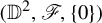
 $(\mathbb {D}^2,\mathscr {F},\{0\})$
be a holomorphic foliation on the unit bidisc
 $\mathbb {D}^2$
defined by the linear vector field
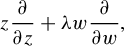
 $Z(z,w)=z ({\partial }/{\partial z})+\unicode{x3bb} w ({\partial }/{\partial w}),$
where
 $\unicode{x3bb} \in \mathbb {C}\backslash \mathbb {R}$
, that is to say,
 $0$
is a hyperbolic singularity. Let T be a harmonic current directed by
 $\mathscr {F}$
which does not give mass to any of the two separatrices
 $(z=0)$
and
 $(w=0)$
. Then the Lelong number of T at
 $0$
vanishes.
Next, Nguyên applies this result to prove the existence of Lyapunov exponents for singular holomorphic foliations on compact projective surfaces [Reference Nguyên20]. Very recently he has proved in [Reference Nguyên19] that for every
 $n\geqslant 2,$
the Lelong numbers of any directed harmonic current which gives no mass to invariant hyperplanes vanishes near weakly hyperbolic singularities in
 $\mathbb {C}^n.$
This result is optimal; see [Reference Dinh and Wu10]. The mass-distribution problem would be completed once we could understand the behaviour of harmonic currents near non-hyperbolic non-degenerate singularities, and near degenerate singularities.
The present paper answers (partly) the problem in the non-hyperbolic linearizable singularity case. Here is our first main result.
Theorem 1.4. Let
 $(\mathbb {D}^2,\mathscr {F},\{0\})$
be a holomorphic foliation on the unit bidisc
 $\mathbb {D}^2$
defined by the linear vector field
 $Z(z,w)=z ({\partial }/{\partial z})+\unicode{x3bb} w ({\partial }/{\partial w})$
, where
 $\unicode{x3bb} \in \mathbb {R}^*$
. Let T be a harmonic current directed by
 $\mathscr {F}$
which does not give mass to any of the two separatrices
 $(z=0)$
and
 $(w=0)$
. Assume
 $T\neq 0$
. Then the Lelong number of T at
 $0$
:
-
• is strictly positive and could be infinite if
$\unicode{x3bb}>0$
; -
• vanishes if
$\unicode{x3bb} \in \mathbb {Q}_{<0}$
.


For the foliation concerned
 $(\mathbb {D}^2,\mathscr {F},\{0\})$
, a local leaf
 $P_\alpha $
, with
 $\alpha \in \mathbb {C}^*$
, can be parametrized by
 $(z,w)=(e^{-v+iu},\alpha e^{-\unicode{x3bb} v+i\unicode{x3bb} u})$
, with
 $u,v\in \mathbb {R}$
. See the parametrization (1) for details. The monodromy group around the singularity is generated by
 $(z,w)\mapsto (z,e^{2\pi i\unicode{x3bb} }w)$
. It is a cyclic group of finite order when
 $\unicode{x3bb} \in \mathbb {Q}^*$
, of infinite order when
 $\unicode{x3bb} \notin \mathbb {Q}$
.
We are now ready to introduce the notion of periodic current, an essential tool in this paper. A directed harmonic current T is called periodic if it is invariant under some cofinite subgroup of the monodromy group, that is, under the action of
 $(z,w)\mapsto (z,e^{2k\pi i \unicode{x3bb} }w)$
for some
 $k\in \mathbb {Z}_{>0}$
.
Observe that if
 $\unicode{x3bb} =({a}/{b})\in \mathbb {Q}^*$
with
 $a\in \mathbb {Z}^*$
,
 $b\in \mathbb {Z}_{>0}$
, then any directed harmonic current is invariant under the action of
 $(z,w)\mapsto (z,e^{2b\pi i \unicode{x3bb} }w)$
, hence is periodic. But when
 $\unicode{x3bb} \notin \mathbb {Q}^*$
, the periodicity is a non-trivial assumption. It does not follow from the ergodicity of irrational rotation because the current is only continuous on leaf parameters
 $(u,v)$
for each fixed
 $\alpha $
. It may not be continuous in variables
 $(z,w)$
.
We are in a position to state our second main result.
Theorem 1.5. Using the same notation as above, the Lelong number of T at the singularity is
 $0$
when
 $\unicode{x3bb} <0$
and the current is periodic, in particular, when
 $\unicode{x3bb} \in \mathbb {Q}_{<0}$
.
It remains open to determine the possible Lelong number values of non-periodic T when
 $\unicode{x3bb} <0$
is irrational.
Section 2 reviews the definition of singular holomorphic foliations, directed harmonic currents, the mass and the Lelong number. Section 3 describes the topology of leaves near linearizable non-hyperbolic singularities, resolves the ambiguity of normalizing harmonic functions on the leaves and provides practical formulas for the mass and the Lelong number. Section 4 calculates the Lelong number when
 $\unicode{x3bb} \in \mathbb {Q}_{>0}$
. Section 5 calculates the Lelong number when
 $\unicode{x3bb} \in \mathbb {R}_{>0}\backslash \mathbb {Q}$
, with an analysis on Poisson integrals of non-periodic currents. Section 6 calculates the Lelong number when
 $\unicode{x3bb} <0$
, assuming that the currents are periodic.
2 Background
2.1 Singularities of holomorphic foliations
To start with, recall the definition of singular holomorphic foliation on a complex surface M.
Definition 2.1. Let
 $E\subset M$
be some closed subset, possibly empty, such that
 $\overline {M\backslash E}=M$
. A singular holomorphic foliation
 $(M,E,\mathscr {F}{\kern1.5pt})$
consists of a holomorphic atlas
 $\{(\mathbb {U}_i,\Phi _i)\}_{i\in I}$
on
 $M\backslash E$
which satisfies the following conditions.
-
(1) For each
$i\in I$
,
$\Phi _i: \mathbb {U}_i\rightarrow \mathbb {B}_i\times \mathbb {T}_i$
is a biholomorphism, where
$\mathbb {B}_i$
and
$\mathbb {T}_i$
are domains in
$\mathbb {C}$
. -
(2) For each pair
$(\mathbb {U}_i,\Phi _i)$
and
$(\mathbb {U}_j,\Phi _j)$
with
$\mathbb {U}_i\cap \mathbb {U}_j\neq \emptyset $
, the transition map has the form
$$ \begin{align*} \Phi_{ij}:=\Phi_i\circ\Phi_j^{-1}:\Phi_j(\mathbb{U}_i\cap\mathbb{U}_j)\rightarrow\Phi_i(\mathbb{U}_i\cap\mathbb{U}_j) \end{align*} $$
where
$$ \begin{align*} \Phi_{ij}(b,t)=(\Omega(b,t),\Lambda(t)), \end{align*} $$
$(b,t)$
are the coordinates on
$\mathbb {B}_j\times \mathbb {T}_j$
, and the functions
$\Omega $
,
$\Lambda $
are holomorphic, with
$\Lambda $
independent of b.


Each open set
 $\mathbb {U}_i$
is called a flow box. For each
 $c\in \mathbb {T}_i$
, the Riemann surface
 $\Phi _i^{-1}\{t=c\}$
in
 $\mathbb {U}_i$
is called a plaque. Property (2) above ensures that in the intersection of two flow boxes, plaques are mapped to plaques.
A leaf L is a minimal connected subset of M such that if L intersects a plaque, it contains that plaque. A transversal is a Riemann surface immersed in M which is transverse to each leaf of M.
The local theory of singular holomorphic foliations is closely related to holomorphic vector fields. One recalls some basic concepts in
 $\mathbb {C}^2$
; see [Reference Brunella5, Reference Fornæss and Sibony11, Reference Nguyên17, Reference Nguyên18].
Definition 2.2. Let
 $Z=P(z,w){\partial }/{\partial z}+Q(z,w){\partial }/{\partial w}$
be a holomorphic vector field defined in a neighbourhood
 $\mathbb {U}$
of
 $(0,0)\in \mathbb {C}^2$
. One says that Z is:
-
(1) singular at
$(0,0)$
if
$P(0,0)=Q(0,0)=0$
; -
(2) linear if it can be written as
where
$$ \begin{align*} Z=\unicode{x3bb}_1 z\frac{\partial}{\partial z}+\unicode{x3bb}_2 w \frac{\partial}{\partial w} \end{align*} $$
$\unicode{x3bb} _1$
,
$\unicode{x3bb} _2\in \mathbb {C}$
are not simultaneously zero;
-
(3) linearizable if it is linear after a biholomorphic change of coordinates.


Suppose the holomorphic vector field
 $Z=P({\partial }/{\partial z})+Q({\partial }/{\partial w})$
admits a singularity at the origin. Let
 $\unicode{x3bb} _1$
,
 $\unicode{x3bb} _2$
be the eigenvalues of the Jacobian matrix
 $\textstyle (\! \begin {smallmatrix} P_z & P_w \\ Q_z & Q_w \end {smallmatrix} \!)$
at the origin.
Definition 2.3. The singularity is non-degenerate if both
 $\unicode{x3bb} _1$
,
 $\unicode{x3bb} _2$
are non-zero. This condition is biholomorphically invariant.
In this paper, all singularities are assumed to be non-degenerate. Then the foliation defined by integral curves of Z has an isolated singularity at
 $0$
. Degenerate singularities are studied in [Reference Brunella5]. Seidenberg’s reduction theorem [Reference Seidenberg21] shows that degenerate singularities can be resolved into non-degenerate ones after finitely many blow-ups.
Definition 2.4. A singularity of Z is hyperbolic if the quotient
 $\unicode{x3bb} :=({\unicode{x3bb} _1}/{\unicode{x3bb} _2})\in \mathbb {C}\backslash \mathbb {R}$
. It is non-hyperbolic if
 $\unicode{x3bb} \in \mathbb {R}^*$
. It is in the Poincaré domain if
 $\unicode{x3bb} \in \mathbb {C}\backslash \mathbb {R}_{\leqslant 0}$
. It is in the Siegel domain if
 $\unicode{x3bb} \in \mathbb {R}_{<0}$
.
One can verify that the quotient is unchanged by multiplication of Z by any non-vanishing holomorphic function.
One could consider
 $\unicode{x3bb} ^{-1}={\unicode{x3bb} _2}/{\unicode{x3bb} _1}$
instead of
 $\unicode{x3bb} $
, but then
 $\unicode{x3bb} \notin \mathbb {R}$
if and only if
 ${\unicode{x3bb} ^{-1}\notin \mathbb {R}}$
. Thus, the notion of hyperbolicity is well defined. Also, being non-hyperbolic, in the Poincaré domain or Siegel domain, is well defined. The complex number
 $\unicode{x3bb} $
will be called an eigenvalue of Z at the singularity, with an inessential abuse due to this exchange
 $\unicode{x3bb} \leftrightarrow \unicode{x3bb} ^{-1}$
. The unordered pair
 $\{\unicode{x3bb} ,\unicode{x3bb} ^{-1}\}$
is invariant under local biholomorphic changes of coordinates.
Consider a holomorphic foliation
 $(M,E,\mathscr {F}{\kern1.5pt})$
where E is discrete. When one tries to linearize a vector field near an isolated non-degenerate singularity, one has to divide power series coefficients by quantities
 $m_1+\unicode{x3bb} m_2-1$
and
 $m_1+\unicode{x3bb} m_2-\unicode{x3bb} $
where
 $m_1$
,
 $m_2\in \mathbb {Z}_{\geqslant 0}$
with
 $m_1+m_2\geqslant 2$
. To ensure convergence, these quantities have to be non-zero and not too close to zero.
These quantities are non-zero if and only if
 $\unicode{x3bb} \notin \mathbb {Q}_{\neq 1}$
. They do not have
 $0$
as a limit if and only if
 $\unicode{x3bb} \notin \mathbb {R}_{\leqslant 0}$
, that is, the singularity is in the Poincaré domain.
We are now ready to state some linearization results in
 $\mathbb {C}^2$
.
Theorem 2.5. (Poincaré; see [Reference Arnold and Ilyashenko2, Ch. 4, §1.2, pp. 72])
A singular holomorphic vector field in
 $\mathbb {C}^2$
is holomorphically equivalent to its linear part if its eigenvalue
 $\unicode{x3bb} \in (\mathbb {C}\backslash \mathbb {R}_{\leqslant 0})\backslash \mathbb {Q}_{\neq 1}$
.
Remark 2.6. The linear part of a singular holomorphic vector field is
 $$ \begin{align*} (az+bw)\frac{\partial}{\partial z}+(cz+dw)\frac{\partial}{\partial w} \end{align*} $$
for some
 $a,b,c,d\in \mathbb {C}$
with
 $ad-bc\neq 0$
if the singularity is assumed to be non-degenerate. It is non-linearizable if and only if the Jordan normal form of the Jacobian matrix
 $\textstyle (\! \begin {smallmatrix} a & b\\ c & d \end {smallmatrix} \!)$
has a rank-2 block
 $\textstyle (\! \begin {smallmatrix} a & 1\\ 0 & a \end {smallmatrix} \!)$
with
 $a\neq 0$
. In this case
 $\unicode{x3bb} =1$
, hence Poincaré’s theorem holds. The vector field is holomorphically equivalent to its linear part
 $(az+w){\partial }/{\partial z}+aw({\partial }/{\partial w})$
, but is not linearizable.
For the resonant case
 $\unicode{x3bb} \in \mathbb {Q}_{\neq {1}}$
and the degenerate case, one may use the Poincaré–Dulac normal form [Reference Arnold and Ilyashenko2, Ch. 3, §3.2, pp. 54].
In particular, all hyperbolic singularities are linearizable.
To get linearization for
 $\unicode{x3bb} $
in the Siegel domain, the following result assumes the more advanced Brjuno condition.
Theorem 2.7. (Brjuno [Reference Arnold and Ilyashenko2, Reference Brjuno4])
A singular holomorphic vector field with a non-resonant linear part is holomorphically linearizable if its eigenvalue
 $\unicode{x3bb} \in \mathbb {R}$
satisfies the condition
 $$ \begin{align*} \sum_{n\geqslant 1}\frac{\log q_{n+1}}{q_n}<\infty, \end{align*} $$
where
 $p_n/q_n$
is the nth approximant of the continued fraction expansion of
 $\unicode{x3bb} $
.
The golden ratio
 $$ \begin{align*} \frac{\sqrt{5}-1}{2}=1+\frac{1}{1+\frac{1}{1+\cdots}} \end{align*} $$
is a Brjuno number. Indeed, any irrational number whose continued fraction expansion ends with a string of 1s
 $$ \begin{align*} \alpha=a_0+\frac{1}{a_1+\frac{1}{\cdots}}=[a_0,a_1,\ldots,a_k,1,1,\ldots]\in\mathbb{R}\backslash\mathbb{Q} \quad(a_0\in\mathbb{Z} ,a_1,\ldots, a_k\in\mathbb{N}), \end{align*} $$
is a Brjuno number. The Brjuno numbers are dense in
 $\mathbb {R}\backslash \mathbb {Q}$
. See [Reference Lee14, Propositions 1.2 and 1.3].
In this paper, all singularities are assumed to be linearizable.
2.2 Directed harmonic currents
Let
 $(\mathbb {D}^2,\mathscr {F},\{0\})$
be a holomorphic foliation on the unit bidisc
 $\mathbb {D}^2$
defined by the linear vector field
 $Z=z{\partial }/{\partial z}+\unicode{x3bb} w({\partial }/{\partial w})$
with
 $\unicode{x3bb} \in \mathbb {R}^*$
. One may assume
 $0<|\unicode{x3bb} |\leqslant 1$
after switching z and w if necessary. There are always two separatrices
 $\{z=0\}$
and
 $\{w=0\}$
. Other leaves can be parametrized as
 $$ \begin{align} L_\alpha:=\{(z,w)=\psi_\alpha(\zeta):= (e^{i \zeta},\alpha e^{i \unicode{x3bb} \zeta})=(e^{-v+i u},\alpha e^{-\unicode{x3bb} v+i \unicode{x3bb} u})\} \quad (\alpha\neq0), \end{align} $$
where
 $\zeta =u+iv\in \mathbb {C}$
. The map
 $$ \begin{align*} \begin{aligned} \Psi:\mathbb{C}\times\mathbb{C}^*&\longrightarrow\mathbb{C}^2\\ (\zeta,\alpha)&\longmapsto (e^{i \zeta},\alpha e^{i \unicode{x3bb} \zeta}) \end{aligned} \end{align*} $$
is locally biholomorphic. Here
 $\alpha $
is the coordinate on the transversal and
 $\zeta $
is the coordinate on leaves. It is not injective since
 $\Psi (\zeta +2\pi ,\alpha )=\Psi (\zeta ,\alpha e^{2\pi i\unicode{x3bb} })$
.
Two numbers
 $\alpha $
,
 $\beta \in \mathbb {C}^*$
are equivalent
 $\alpha \sim \beta $
if
 $\beta =e^{2k\pi i \unicode{x3bb} }\alpha $
for some
 $k\in \mathbb {Z}$
. The following statements are equivalent:
-
•
$\alpha \sim \beta $
; -
•
$L_\alpha =L_\beta $
; -
•
$\psi _\alpha =\psi _\beta \circ (\text {translation of }2k\pi )$
for some
$k\in \mathbb {Z}$
.


Let
 $\mathscr {C}_{\mathscr {F}}$
(respectively,
 $\mathscr {C}_{\mathscr {F}}^{1,1}$
) denote the space of functions (respectively, forms of bidegree
 $(1,1)$
) defined on leaves of the foliation which are compactly supported on
 $M\backslash E$
, leafwise smooth and transversally continuous. A form
 $\iota \in \mathscr {C}_{\mathscr {F}}^{1,1}$
is said to be positive if its restriction to every plaque is a positive (1,1)-form.
A directed harmonic current T on
 $\mathscr {F}$
is a continuous linear form on
 $\mathscr {C}_{\mathscr {F}}^{1,1}$
satisfying the following two conditions:
-
(1)
$i\partial \bar {\partial } T=0$
in the weak sense, that is,
$T(i\partial \bar {\partial }f)=0$
for all
$f\in \mathscr {C}_{\mathscr {F}}$
, where in the expression
$i\partial \bar {\partial }f$
one only considers
$\partial \bar {\partial }$
along the leaves; -
(2) T is positive, that is,
$T(\iota )\geqslant 0$
for all positive forms
$\iota \in \mathscr {C}_{\mathscr {F}}^{1,1}$
.


It is well known (see, for example, [Reference Berndtsson and Sibony3, Reference Dinh, Nguyên and Sibony6, Reference Fornæss and Sibony11]) that a directed harmonic current T on a flow box
 $\mathbb {U}\cong \mathbb {B}\times \mathbb {T}$
can be locally expressed as
 $$ \begin{align} T=\int_{\alpha\in\mathbb{T}} h_\alpha [P_\alpha]\, d\mu(\alpha). \end{align} $$
The
 $h_\alpha $
are non-negative harmonic functions on the local leaves
 $P_\alpha $
and
 $\mu $
is a Borel measure on the transversal
 $\mathbb {T}$
. If
 $h_\alpha =0$
at some point on
 $P_\alpha $
, then by the mean value theorem
 $h_\alpha \equiv 0$
. For all such
 $\alpha \in \mathbb {T}$
, we replace
 $h_\alpha $
by the constant function
 $1$
and we set
 $d\mu (\alpha )=0$
. Thus, we get a new expression of T where
 $h_\alpha>0$
for all
 $\alpha \in \mathbb {T}$
.
Such an expression is not unique since
 $T=\int _{\alpha \in \mathbb {T}}(h_\alpha g(\alpha ))[P_\alpha ](({1}/{g(\alpha )})\, d\mu (\alpha ))$
for any measurable positive function
 $g:\mathbb {T}\rightarrow \mathbb {R}_{>0}$
which is finite and non-zero almost everywhere. The expression is unique after normalization, which means that for each
 $\alpha \in \mathbb {T}$
one fixes
 $h_\alpha (z_0,w_0)=1$
at some point
 $(z_0,w_0)\in P_\alpha $
.
Each harmonic function
 $h_\alpha $
on the leaf
 $V_\alpha $
can be pulled back by the parametrization
 $\Psi $
as the harmonic function
 $$ \begin{align*} H_\alpha(u,v):=h_\alpha(e^{-v+iu},\alpha e^{-\unicode{x3bb} v+i\unicode{x3bb} u}). \end{align*} $$
The domain of definition for u, v will be precisely described later in this section.
In §1 the notion of periodic current was introduced. Here is an equivalent characterization.
Proposition 2.8. A directed harmonic current T is periodic if and only if there exists some
 $k\in \mathbb {Z}_{>0}$
such that
 $H_\alpha (u+2 k\pi ,v)=H_\alpha (u,v)$
for all
 $u,v$
and for
 $\mu $
-almost all
 $\alpha $
.
Proof. By definition T is invariant under
 $(z,w)\mapsto (z,e^{2k\pi i \unicode{x3bb} }w)$
for some
 $k\in \mathbb {Z}_{>0}$
, which is equivalent to
 $H_\alpha (u+2 k\pi ,v)=H_\alpha (u,v)$
for all
 $u,v$
and
 $\mu $
-almost all
 $\alpha $
.
A current T of the form (2) is
 $dd^c$
-closed on
 $\mathbb {D}^2\backslash \{0\}$
. But its trivial extension
 $\tilde {T}$
across the singularity
 $0$
is not necessarily
 $dd^c$
-closed on
 $\mathbb {D}^2$
. It is true when T is compactly supported, for example when T is a localization of a current on a compact manifold, by the following argument (see [Reference Dinh, Nguyên and Sibony6, Lemma 2.5] for details).
Let T be a directed harmonic current on
 $M\backslash E$
, where M is a compact complex manifold and E is a finite set. The current T can be extended by zero through E in order to obtain the positive current
 $\tilde T$
on M. Next, we apply the following result.
Theorem 2.9. (Alessandrini and Bassanelli [Reference Alessandrini and Bassanelli1, Theorem 5.6])
Let
 $\Omega $
be an open subset of
 $\mathbb {C}^n$
and Y an analytic subset of
 $\Omega $
of dimension less than p. Suppose T is a negative current of bidimension
 $(p,p)$
on
 $\Omega \backslash Y$
such that
 $dd^c T\geqslant 0$
. Then the following assertions hold.
-
(1) The mass of T near Y is locally finite. In particular, T admits a trivial extension by
$0$
across Y, denoted by
$\tilde {T}$
. -
(2)
$dd^c\tilde {T}\geqslant 0$
on
$\Omega $
.


Here
 $-T$
is a negative current of bidimension
 $(1,1)$
on
 $M\backslash E$
with
 $dd^c (-T)\geqslant 0$
and E has dimension
 $0$
. So for the trivial extension
 $\tilde {T}$
on M one has
 $dd^c(-\tilde {T})\geqslant 0$
. Moreover,
 $\tilde {T}$
is compactly supported since M is compact. Thus
 $$ \begin{align*} \langle dd^c\tilde{T},1 \rangle = \langle \tilde{T},dd^c1 \rangle = 0. \end{align*} $$
Combining with
 $dd^c\tilde {T}\leqslant 0$
from the extension theorem, one concludes that
 $dd^c\tilde {T}=0$
on M. Thus, locally near any singularity, the trivial extension
 $\tilde {T}$
is
 $dd^c$
-closed.
Let
 $\beta :=idz\wedge d\bar {z}+idw\wedge d\bar {w}$
be the standard Kähler form on
 $\mathbb {C}^2$
. The mass of T on a domain
 $U\subset \mathbb {D}^2$
is denoted by
 $\|T\|_U:=\int _U T\wedge \beta $
. In this paper, all currents are assumed to have finite mass on
 $\mathbb {D}^2$
.
Definition 2.10. (See [Reference Nguyên19, §2.4])
Let T be a directed harmonic current on
 $(\mathbb {D}^2,\mathscr {F},\{0\})$
. We define the Lelong number by the limit
 $$ \begin{align*} \mathscr{L}(T,0)=\limsup\limits_{r\rightarrow0+}\frac{1}{\pi r^2}\|T\|_{r\mathbb{D}^2}\in[0,+\infty]. \end{align*} $$
The limit can be infinite when the trivial extension
 $\tilde {T}$
across the origin is not
 $dd^c$
-closed [Reference Nguyên19, Example 2.11]. When
 $\tilde {T}$
is
 $dd^c$
-closed, the following theorem ensures the finiteness.
Theorem 2.11. (Skoda [Reference Skoda22])
Let T be a positive
 $dd^c$
-closed
 $(1,1)$
-current in
 $\mathbb {D}^2$
. Then the function
 $r\mapsto {1}/{\pi r^2}\|T\|_{r\mathbb {D}^2}$
is increasing with
 $r\in (0, 1]$
.
In our case, the function
 $$ \begin{align*} r\mapsto \frac{1}{\pi r^2}\|\tilde{T}\|_{r\mathbb{D}^2}=\frac{1}{\pi r^2}\|T\|_{r\mathbb{D}^2} \end{align*} $$
is increasing with
 $r\in (0, 1]$
. In particular,
 $$ \begin{align*} \mathscr{L}(T,0)=\lim\limits_{r\rightarrow0+}\frac{1}{\pi r^2}\|T\|_{r\mathbb{D}^2}\in\bigg[0,\dfrac{1}{\pi}\|T\|_{\mathbb{D}^2}\bigg]. \end{align*} $$
In this paper, the symbols
 $\lesssim $
and
 $\gtrsim $
stand for inequalities up to a multiplicative positive constant depending only on
 $\unicode{x3bb} $
. We write
 $\approx $
when both inequalities are satisfied.
3 Parametrization of leaves
Recall the parametrization of an arbitrary leaf
 $L_\alpha $
:
 $$ \begin{align*} \psi_\alpha(\zeta)=\Psi(\zeta,\alpha)=(e^{i \zeta},\alpha e^{i \unicode{x3bb} \zeta}) \quad(\alpha\in\mathbb{C}^*,\zeta\in\mathbb{C}). \end{align*} $$
To calculate the mass
 $\|T\|_{\mathbb {D}^2}$
and the Lelong number
 $\mathscr {L}(T,0)$
, we shall study
 $\Psi ^{-1}(r \mathbb {D}^2)$
for
 $r\in (0,1]$
. Define
 $P_\alpha :=L_\alpha \cap \mathbb {D}^2$
and
 $P_\alpha ^{(r)}:=L_\alpha \cap r \mathbb {D}^2$
. Define
 $\log ^+(x):=\max \{0,\log (x)\}$
for
 $x>0$
.
Lemma 3.1. The range of
 $(u,v)$
for a point
 $(z,w)\in P_\alpha $
and
 $P_{\alpha }^{(r)}$
is an upper half-plane when
 $\unicode{x3bb}>0$
, or a horizontal strip when
 $\unicode{x3bb} <0$
. More precisely:
-
(1) when
$\unicode{x3bb}>0$
,
$$ \begin{align*} (z,w)\in P_\alpha & \Longleftrightarrow\, v>\frac{\log^+|\alpha|}{\unicode{x3bb}},\\ (z,w)\in P_\alpha^{(r)} & \Longleftrightarrow \left\{ \begin{aligned} &v>\frac{\log|\alpha|-\log r}{\unicode{x3bb}} & (|\alpha|\geqslant r^{1-\unicode{x3bb}}),\\ &v>-\log r & (|\alpha|<r^{1-\unicode{x3bb}}); \end{aligned} \right. \end{align*} $$
-
(2) when
$\unicode{x3bb} <0$
,
$P_\alpha =\emptyset $
for
$|\alpha |\geqslant 1$
,
$P_\alpha ^{(r)}=\emptyset $
for
$|\alpha |\geqslant r^{1-\unicode{x3bb} }$
and for the other
$\alpha $
,
$$ \begin{align*} (z,w)\in P_\alpha & \Longleftrightarrow\, 0<v<\frac{\log|\alpha|}{\unicode{x3bb}},\\ (z,w)\in P_\alpha^{(r)} & \Longleftrightarrow -\log r<v<\frac{\log|\alpha|-\log r}{\unicode{x3bb}}. \end{align*} $$


Proof. Recall that
 $(z,w)=(e^{-v+i u},\alpha e^{-\unicode{x3bb} v+i \unicode{x3bb} u})$
on
 $L_{\alpha }$
. So for any
 $r\in (0,1]$
,
 $(z,w)\in P_\alpha ^{(r)}$
if and only if both
 $|z|=e^{-v}<r$
and
 $|w|=|\alpha | e^{-\unicode{x3bb} v}<r$
.
When
 $\unicode{x3bb}>0$
one has
 $v>-\log r$
and
 $v>({\log |\alpha |-\log r})/{\unicode{x3bb} }$
. In particular, for
 $r=1$
, one has
 $v>0$
and
 $v>{\log |\alpha |}/{\unicode{x3bb} }$
.
When
 $\unicode{x3bb} <0$
one has
 $-\log r<v<({\log |\alpha |-\log r})/{\unicode{x3bb} }$
. In particular, for
 $r=1$
, one has
 $0<v<{\log |\alpha |}/{\unicode{x3bb} }$
. If there is no solution for v then
 $P_{\alpha }^{(r)}=\emptyset $
.
When
 $\unicode{x3bb}>0$
, the range of v is unbounded for each fixed
 $\alpha \in \mathbb {C}^*$
. See Figures 1 and 2.
When
 $\unicode{x3bb} <0$
, the range of v is bounded for each fixed
 $\alpha $
. See Figures 3 and 4.
The region of
 $(|\alpha |,v)$
for
 $P_\alpha $
.

The region of
 $(|\alpha |,v)$
for
 $P_\alpha ^{(r)}$
.

The region of
 $(|\alpha |,v)$
for
 $P_\alpha $
.

The region of
 $(|\alpha |,v)$
for
 $P_\alpha ^{(r)}$
.

Case
 $|\alpha |<1$
.

3.1 Positive case
$\unicode{x3bb}>0$

For any
 $\alpha \in \mathbb {C}^*$
fixed, the leaf
 $L_\alpha $
is contained in a real three-dimensional Levi flat CR manifoldFootnote
1
 $|w|=|\alpha | |z|^{\unicode{x3bb} }$
, which can be viewed as a curve in
 $|z|=e^{-v}$
,
 $|w|=|\alpha | e^{-\unicode{x3bb} v}$
coordinates. The norms
 $|z|$
and
 $|w|$
depend only on v. When
 $v\rightarrow +\infty $
, the point on the leaf tends to the singularity
 $(0,0)$
described by Figures 5 and 6.
Case
 $|\alpha |\geqslant 1$
.

If one fixes some
 $v=-\log r$
, then
 $|z|=r$
and
 $|w|=|\alpha | r^\unicode{x3bb} $
is fixed. The set
 $\mathbb {T}^2_r:=\{(z,w)\in \mathbb {D}^2:|z|=r,|w|=|\alpha | r^\unicode{x3bb} \}$
is a torus and the intersection of the leaf
 $L_\alpha $
with this torus is a smooth curve
 $L_{\alpha ,r}:=L_\alpha \cap \mathbb {T}^2_r$
.
When
 $\unicode{x3bb} \in \mathbb {Q}$
, this curve
 $L_{\alpha ,r}$
is closed. See Figure 7.
When
 $\unicode{x3bb} \notin \mathbb {Q}$
, this curve
 $L_{\alpha ,r}$
is dense on the torus
 $\mathbb {T}_r^2$
. See Figures 8 and 9.
In this case the two curves
 $L_{\alpha ,r}$
and
 $L_{\alpha e^{2\pi i \unicode{x3bb} },r}$
are two different parametrizations of the same image. The dashed curve in Figure 8 is not only the image of
 $L_{\alpha ,r}$
for
 $u\in [2\pi ,4\pi )$
but also the image of
 $L_{\alpha e^{2\pi i \unicode{x3bb} },r}$
for
 $u\in [0,2\pi )$
. This raises ambiguity while normalizing harmonic functions on a leaf
 $L_\alpha $
.
Such ambiguity can be resolved once one restricts everything to an open subset
 $U_\epsilon :=\{(z,w)\in \mathbb {D}^2~|~{\textrm {arg}}(z)\in (0,2\pi -\epsilon ),z\neq 0,w\neq 0\}$
for some fixed
 $\epsilon \in [0,\pi )$
. Any leaf
 $L_\alpha $
on
 $U_\epsilon $
decomposes into a disjoint union of infinitely many components:
 $$ \begin{align*} L_\alpha\cap U_\epsilon=\bigcup\limits_{k\in\mathbb{Z}}\!\bigg\{(e^{-v+iu},\alpha e^{2k\pi i\unicode{x3bb}} e^{-\unicode{x3bb} v+i\unicode{x3bb} u})~|~u\kern1.2pt{\in}\kern1.2pt(0,2\pi-\epsilon),v\kern1.2pt{>}\kern1.2pt\frac{\log^+|\alpha|}{\unicode{x3bb}}\bigg\}. \end{align*} $$
For example, in Figure 10, the curve and the dashed curve are two distinct components of
 $L_{1,1}\cup U_{\epsilon}$
.
A closed curve on a torus.

Two loops.

Twenty loops.

Two components of
 $L_{1,1}\cup U_{\epsilon}$
.

Such a parametrization is yet not unique. For example, for any
 $k_0\in \mathbb {Z}$
one can parametrize
 $$ \begin{align*} L_\alpha\cap U_\epsilon=\bigcup\limits_{k\in\mathbb{Z}}\!\bigg\{\!(e^{-v+iu},\alpha e^{2k\pi i\unicode{x3bb}} e^{-\unicode{x3bb} v+i\unicode{x3bb} u})\kern1.2pt{|}\kern1.2pt u\kern1.2pt{\in}\kern1.2pt(2k_0\pi,2k_0\pi+2\pi-\epsilon),v>\frac{\log^+|\alpha|}{\unicode{x3bb}}\bigg\}\kern-1pt. \end{align*} $$
The parametrization is unique once one fixes
 $k_0$
, for example,
 $k_0=0$
. I remark for the time being that all other choices of
 $k_0$
will be used for analysing non-periodic currents in §5.2.
3.2 Resolving ambiguity in the irrational case
Let
 $\unicode{x3bb} \notin \mathbb {Q}$
. Let T be a harmonic current directed by
 $\mathscr {F}$
. Then
 $T|_{P_\alpha }$
has the form
 $h_\alpha (z,w)[P_\alpha ]$
. One may assume that
 $h_\alpha $
is nowhere 0 for every
 $\alpha $
. Let
 $$ \begin{align*} H_\alpha(u+iv):=h_\alpha\circ \psi_\alpha\bigg(u+iv+i\frac{\log^+|\alpha|}{\unicode{x3bb}}\bigg). \end{align*} $$
This is a positive harmonic function for
 $\mu $
-almost all
 $\alpha \in \mathbb {C}^*$
defined in a neighbourhood of the upper half-plane
 $\mathbb {H}=\{(u+iv)\in \mathbb {C}~|~v>0\}$
, determined by the Poisson integral formula
 $$ \begin{align*} H_\alpha(u+iv)=\frac{1}{\pi} \int_{y\in\mathbb{R}}H_\alpha(y) \frac{v} {v^2+(y-u)^2} dy+C_\alpha v. \end{align*} $$
One can normalize
 $H_\alpha $
by setting
 $H_\alpha (0)=1$
. But by doing so one may normalize data over the same leaf for multiple times. Indeed, any pair of equivalent numbers
 $\alpha \sim \beta $
in
 $\mathbb {C}^*$
,
 $\beta =\alpha e^{2k\pi i \unicode{x3bb} }$
, may provide us with two different normalizations
 $H_{\alpha }$
and
 $H_{\beta }$
on the same leaf
 $L_{\alpha }=L_{\beta }$
. A major task is to find formulas for the mass and the Lelong number independent by the choice of normalization.
The ambiguity is described by the following proposition.
Proposition 3.2. If
 $\beta =\alpha e^{2k \pi i \unicode{x3bb} }$
for some
 $k\in \mathbb {Z}$
, then the two normalized positive harmonic functions
 $H_\alpha $
and
 $H_\beta $
satisfy
 $$ \begin{align*} H_\alpha(u+iv) = H_\alpha(2k\pi) H_\beta(u-2k\pi+iv). \end{align*} $$
In other words, they differ by a translation and a multiplication by a non-zero constant.
Proof. When
 $|\alpha |<1$
, by definition
 $$ \begin{align*} H_\alpha(u+iv)=h_\alpha(e^{-v+iu},\alpha e^{-\unicode{x3bb} v+i \unicode{x3bb} u}), \quad H_\alpha(0)=h_\alpha(1,\alpha). \end{align*} $$
Thus, the normalized harmonic function is
 $$ \begin{align*} H_\alpha(u+iv)=\frac{h_\alpha(e^{-v+iu},\alpha e^{-\unicode{x3bb} v+i \unicode{x3bb} u})}{h_\alpha(1,\alpha)}, \end{align*} $$
and for the same reason
 $$ \begin{align*}H_\beta(u+iv)=\frac{h_\beta(e^{-v+iu},\beta e^{-\unicode{x3bb} v+i \unicode{x3bb} u})}{h_\beta(1,\beta)}. \end{align*} $$
The two functions
 $h_\alpha $
and
 $h_\beta $
are the positive harmonic coefficient of T on the same leaf
 $L_\alpha =L_\beta $
, hence they differ up to multiplication by a positive constant
 $C>0$
:
 $$ \begin{align*} \begin{aligned} h_\alpha(e^{-v+iu},\alpha e^{-\unicode{x3bb} v+i \unicode{x3bb} u})&=C\cdot h_\beta(e^{-v+iu},\alpha e^{-\unicode{x3bb} v+i \unicode{x3bb} u})\\ &=C\cdot h_\beta(e^{-v+iu},\beta e^{-2k \pi i \unicode{x3bb}} e^{-\unicode{x3bb} v+i \unicode{x3bb} u})\\ &=C\cdot h_\beta(e^{-v+i(u-2k \pi)},\beta e^{-\unicode{x3bb} v+i \unicode{x3bb} (u-2k \pi)}). \end{aligned} \end{align*} $$
Thus,
 $$ \begin{align*} \begin{aligned} H_\alpha(u+iv)&=\frac{h_\alpha(e^{-v+iu},\alpha e^{-\unicode{x3bb} v+i \unicode{x3bb} u})}{h_\alpha(1,\alpha)}=\frac{C\cdot h_\beta(e^{-v+i(u-2k \pi)},\beta e^{-\unicode{x3bb} v+i \unicode{x3bb} (u-2k \pi)})}{C\cdot h_\beta(1,\alpha)}\\ &=\frac{h_\beta(e^{-v+i(u-2k \pi)},\beta e^{-\unicode{x3bb} v+i \unicode{x3bb} (u-2k \pi)})}{h_\beta(1,\beta)}\cdot \frac{h_\beta(1,\beta)}{h_\beta(1,\alpha)}\\ &=H_\beta(u-2k \pi+iv)\cdot \frac{h_\beta(1,\beta)}{h_\beta(1,\alpha)}. \end{aligned} \end{align*} $$
When
 $u=2k \pi $
and
 $v=0$
one has
 $H_\alpha (2k \pi )={h_\beta (1,\beta )}/{h_\beta (1,\alpha )}$
. Thus, one gets the equality. The proof for the case
 $|\alpha |>1$
is similar.
Take the open subset
 $U:=\{(z,w)\in \mathbb {D}^2~|~z\notin \mathbb {R}_{\geqslant 0},w\neq 0\}$
. See Figures 11 and 12.
Domain U in coordinates
 $(z,w)$
.

Domain U in coordinates
 $(u,v)$
.

Any leaf
 $L_\alpha $
in U is a disjoint union of infinitely many components. Once
 $\alpha $
is fixed, there is a one-to-one correspondence between these components and strips in Figure 12.
 $$ \begin{align*} L_\alpha\cap U=\bigcup\limits_{k\in\mathbb{Z}}\tilde{L}_{\alpha e^{2k\pi i\unicode{x3bb}}}:=\bigcup\limits_{k\in\mathbb{Z}}\!\bigg\{(e^{-v+iu},\alpha e^{2k\pi i\unicode{x3bb}} e^{-\unicode{x3bb} v+i\unicode{x3bb} u})\kern1.2pt{|}\kern1.2pt u\kern1.2pt{\in}\kern1.2pt(0,2\pi),v\kern1.2pt{>}\kern1.2pt\frac{\log^+|\alpha|}{\unicode{x3bb}}\bigg\}. \end{align*} $$
Normalizing
 $H_{\alpha e^{2k\pi i\unicode{x3bb} }}$
on
 $\tilde {L}_{\alpha e^{2k\pi i\unicode{x3bb} }}$
avoids ambiguity. Thus, the mass
 $$ \begin{align*} \begin{aligned} \|T\|_{U}&=\int_{(z,w)\in U}T\wedge i\partial\bar{\partial}(|z|^2+|w|^2)\\ &=\int_{\alpha\in\mathbb{C}^*}\int_{v>{\log^+|\alpha|}/{\unicode{x3bb}}}\int_{u=0}^{2\pi}H_{\alpha}(u+iv) 2(e^{-2v}+\unicode{x3bb}^2 |\alpha|^2 e^{-2\unicode{x3bb} v}) \,du\, dv\, d\mu(\alpha)\\ &=\int_{\alpha\in\mathbb{C}^*}\int_{v>0}\int_{u=0}^{2\pi}H_{\alpha}(u+iv)\|\psi_\alpha'\|^{2}\, du\, dv\, d\mu(\alpha) \end{aligned} \end{align*} $$
for some positive measure
 $\mu $
on
 $\mathbb {C}^*$
. Here,
 $\|\psi _\alpha '\|^2$
is the jacobian coming from the
 $(1,1)$
-form
 $i\partial \bar {\partial }(|z|^2+|w|^2)$
on
 $L_\alpha $
after a change of coordinates and a translation on v:
 $$ \begin{align} \|\psi_\alpha'\|^2=\left\{ \begin{aligned} &2(e^{-2v}+\unicode{x3bb}^2 |\alpha|^2 e^{-2\unicode{x3bb} v}) & (|\alpha|< 1),\\ &2(|\alpha|^{-{2}/{\unicode{x3bb}}}e^{-2v}+\unicode{x3bb}^2 e^{-2\unicode{x3bb} v}) & (|\alpha|\geqslant 1). \end{aligned} \right. \end{align} $$
Since H is harmonic in a neighbourhood of
 $\mathbb {H}$
, it is continuous in
 $\mathbb {H}$
. So
 $$ \begin{align*} \begin{aligned} \|T\|_{U}&=\lim\limits_{\epsilon\rightarrow 0+}\int_{\alpha\in\mathbb{C}^*}\int_{v>0}\int_{u=0}^{2\pi+\epsilon}H_{\alpha}(u+iv)\|\psi_\alpha'\|^2 \,du\, dv\, d\mu(\alpha)\\ &=\lim\limits_{\epsilon\rightarrow0+}\|T\|_{\bigcup\limits_{k\in\mathbb{Z}}\tilde{L}_{\alpha e^{2k \pi i\unicode{x3bb}}}}\\ &=\|T\|_{\mathbb{D}^2}. \end{aligned} \end{align*} $$
Thus, we can express the mass by a formula independent of the choice of normalization
 $$ \begin{align*} \|T\|_{\mathbb{D}^2}=\int_{\alpha\in\mathbb{C}^*}\int_{v>0}\int_{u=0}^{2\pi}H_{\alpha}(u+iv)\|\psi_\alpha'\|^2 \,du\, dv\, d\mu(\alpha). \end{align*} $$
Lemma 3.3. For each
 $k_0\in \mathbb {Z}$
fixed,
 $$ \begin{align} \|T\|_{\mathbb{D}^2}=\int_{\alpha\in\mathbb{C}^*}\int_{v>0}\int_{u=2k_0\pi}^{2k_0\pi+2\pi}H_{\alpha}(u+iv)\|\psi_\alpha'\|^2 \,du \,dv \,d\mu(\alpha). \end{align} $$
Proof. The disjoint union
 $L_\alpha \cap U=\bigcup \nolimits _{k\in \mathbb {Z}}\tilde {L}_{\alpha e^{2k\pi i\unicode{x3bb} }}$
can be parametrized in many other ways. For instance,
 $$ \begin{align*} L_\alpha\cap U=\bigcup\limits_{k\in\mathbb{Z}}\bigg\{(e^{-v+iu},\alpha e^{2k\pi i\unicode{x3bb}} e^{-\unicode{x3bb} v+i\unicode{x3bb} u})~|~u\in(2k_0\pi,2k_0\pi+2\pi),v>\dfrac{\log^+|\alpha|}{\unicode{x3bb}}\bigg\}. \end{align*} $$
By the same argument as above one concludes.
3.3 Negative case
$\unicode{x3bb} <0$

As in the positive case, for any
 $\alpha \in \mathbb {C}^*$
fixed, the leaf
 $L_\alpha $
is contained in a real three-dimensional analytic Levi-flat CR manifold
 $|w|=|\alpha | |z|^{\unicode{x3bb} }$
, which can be viewed as a curve in
 $|z|,|w|$
coordinates. The norms
 $|z|$
and
 $|w|$
depend only on v.
The difference is that in the negative case, no leaf
 $L_\alpha $
tends to the singularity
 $(0,0)$
. For r sufficiently small, the leaf
 $L_\alpha $
is outside of
 $r \mathbb {D}^2$
. See Figure 13.
Case
 $\unicode{x3bb} <0$
.

Like the positive case
 $\unicode{x3bb}>0$
, when one fixes
 $|z|=r$
for some
 $r\in (0,1)$
,
 $|w|=|\alpha | |z|^\unicode{x3bb} $
is uniquely determined and the real two-dimensional leaf
 $L_\alpha $
becomes a real 1-dimensional curve
 $L_{\alpha ,r}:=L_\alpha \cap \mathbb {T}^2_r$
on the torus
 $\mathbb {T}^2_r:=\{(z,w)\in \mathbb {D}^2~|~|z|=r,|w|=|\alpha | r^\unicode{x3bb} \}$
. It is a closed curve if
 $\unicode{x3bb} \in \mathbb {Q}$
, and a dense curve on
 $\mathbb {T}^2_r$
if
 $\unicode{x3bb} \notin \mathbb {Q}$
.
Let T be a harmonic current directed by
 $\mathscr {F}$
. Then
 $T|_{P_\alpha }$
has the form
 $h_\alpha (z,w)[P_\alpha ]$
. Let
 $H_\alpha :=h_\alpha \circ \psi _\alpha (u+iv)$
. It is a positive harmonic function for
 $\mu $
-almost all
 $\alpha \in \mathbb {D}^*$
defined on a neighbourhood of a horizontal strip
 $\{(u,v)\in \mathbb {R}^2~|~0<v<{\log |\alpha |}/{\unicode{x3bb} }\}$
.
As in the case
 $\unicode{x3bb}>0$
, one only calculates the mass on an open subset
 $U:=\{(z,w)\in \mathbb {D}^2~|~z\notin \mathbb {R}_{\geqslant 0},w\neq 0\}$
. For each
 $\alpha \in \mathbb {D}^*$
one normalizes
 $H_\alpha $
by setting
 $H_\alpha (0)=1$
to fix the expression
 $T:=\int h_\alpha [P_\alpha ]\, d\mu (\alpha )$
. Similarly to Lemma 3.3, for each
 $k_0\in \mathbb {Z}$
fixed,
 $$ \begin{align*} \begin{aligned} \|T\|_{\mathbb{D}^2} &=\int_{0<|\alpha|<1}\!\int_{v=0}^{{\log|\alpha|}/{\unicode{x3bb}}}\!\int_{u=2 k_0 \pi}^{2 k_0 \pi+2 \pi}\!\kern-1.2pt H_\alpha(u+iv) 2 (e^{-2v}+\unicode{x3bb}^2 |\alpha|^2 e^{-2\unicode{x3bb} v}) \,du \,dv\, d\mu(\alpha),\\ \mathscr{L}(T,0)&=\lim\limits_{r\rightarrow 0+}\frac{1}{r^2}\|T\|_{r\mathbb{D}^2}\\ & =\lim\limits_{r\rightarrow 0+}\frac{1}{r^2}\int_{0<|\alpha|<r^{1-\unicode{x3bb}}}\int_{v=-\log r}^{({\log|\alpha|-\log r})/{\unicode{x3bb}}}\int_{u=2 k_0 \pi}^{2 k_0 \pi+2 \pi} \\&\qquad\qquad\qquad\ \kern1pt\qquad\qquad H_\alpha(u+iv) 2 (e^{-2v}+\unicode{x3bb}^2 |\alpha|^2 e^{-2\unicode{x3bb} v}) \,du \,dv \,d\mu(\alpha). \end{aligned} \end{align*} $$
These formulas will be calculated in later sections.
4 Positive rational case:
$\unicode{x3bb} =({a}/{b})\in \mathbb {Q}$
,
$\unicode{x3bb} \in (0,1]$


Write
 $\unicode{x3bb} ={a}/{b}$
where
 $a,b\in \mathbb {Z}_{\geqslant 1}$
are coprime. Then in
 $\mathbb {D}^2$
, for any
 $\alpha \in \mathbb {C}^*$
, the union
 $L_\alpha \cup \{0\}$
is the algebraic curve
 $\{w^b=\alpha ^b z^a\}\cap \mathbb {D}^2$
. In other words, every leaf is a separatrix. In this section it will be shown that any directed harmonic current T has non-zero Lelong number.
The parametrization map
 $\psi _\alpha (\zeta ):=(e^{i\zeta },\alpha e^{i\unicode{x3bb} \zeta })$
is now periodic:
 $\psi _\alpha (\zeta +2\pi b)=\psi _\alpha (\zeta )$
. Let T be a directed harmonic current. Then
 $T|_{P_\alpha }$
has the form
 $h_\alpha (z,w)[P_\alpha ]$
. Let
 $$ \begin{align*} H_\alpha(u+iv):=h_\alpha\circ\psi_\alpha\bigg(u+iv+i\frac{\log^+|\alpha|}{\unicode{x3bb}}\bigg). \end{align*} $$
This is a positive harmonic function for
 $\mu $
-almost all
 $\alpha \in \mathbb {C}^*$
defined in a neighbourhood of the upper half-plane
 $\mathbb {H}:=\{(u+iv)\in \mathbb {C}~|~v>0\}$
. Moreover, it is periodic:
 $H_\alpha (u+iv)=H_\alpha (u+2\pi b+iv)$
. Periodic harmonic functions can be characterized by the following lemma.
Lemma 4.1. Let
 $F(u,v)$
be a harmonic function in a neighbourhood of
 $\mathbb {H}$
. If
 $F(u,v)=F(u+2\pi b,v)$
for all
 $(u,v)\in \mathbb {H}$
, then
 $$ \begin{align*} F(u,v)=\sum\limits_{k\in\mathbb{Z},k\neq 0}\bigg(a_k e^{{kv}/{b}}\cos\bigg(\frac{ku}{b}\bigg)+b_k e^{{kv}/{b}}\sin\bigg(\frac{ku}{b}\bigg)\bigg)+a_0+b_0 v, \end{align*} $$
for some
 $a_k$
,
 $b_k\in \mathbb {R}$
. Moreover, if
 $F|_{\mathbb {H}}\geqslant 0$
, then
 $a_0,b_0\geqslant 0$
.
Proof. By periodicity
 $$ \begin{align*} F(u,v)=\sum\limits_{k=1}^{\infty}\bigg(A_k(v) \cos\bigg(\frac{ku}{b}\bigg)+B_k(v) \sin\bigg(\frac{ku}{b}\bigg)\bigg)+A_0(v), \end{align*} $$
for some functions
 $A_k(v)$
,
 $B_k(v)$
. They are smooth since F is harmonic. Moreover,
 $$ \begin{align*} \begin{aligned} 0&=\Delta F(u,v)\\ &=\sum\limits_{k=1}^{\infty}\!\bigg(\!\bigg(A_k''(v)\kern1.2pt{-}\kern1.2pt\bigg(\frac{k}{b}\bigg)^2 A_k(v)\!\bigg)\!\cos\!\bigg(\frac{ku}{b}\bigg)+\bigg(\!B_k''(v)\kern1.2pt{-}\kern1.2pt\bigg(\frac{k}{b}\bigg)^2 B_k(v)\!\bigg)\!\sin\!\bigg(\frac{ku}{b}\bigg)\!\bigg)+A_0''(v). \end{aligned} \end{align*} $$
Thus,
 $$ \begin{align*} A_k''(v)=\bigg(\frac{k}{b}\bigg)^2 A_k(v), \quad B_k''(v)=\bigg(\frac{k}{b}\bigg)^2 B_k(v), \quad A_0''(v)=0. \end{align*} $$
Hence,
 $$ \begin{align*} A_k(v)=a_k e^{{kv}/{b}}+a_{-k} e^{-{kv}/{b}}, \quad B_k(v)=b_k e^{{kv}/{b}}-b_{-k} e^{-{kv}/{b}}, \quad A_0(v)=a_0+b_0 v, \end{align*} $$
for some
 $a_k$
,
 $a_{-k}$
,
 $b_k$
,
 $b_{-k}\in \mathbb {R}$
. One obtains the equality.
If
 $F|_{\mathbb {H}}\geqslant 0$
, then for any
 $v\geqslant 0$
,
 $$ \begin{align*} \int_{u=0}^{2\pi b}F(u,v)\,du=2\pi b(a_0+b_0 v)\geqslant0. \end{align*} $$
Thus,
 $a_0,b_0\geqslant 0.$
For
 $\alpha ,\beta \in \mathbb {C}^*$
, the two maps
 $\psi _\alpha $
and
 $\psi _\beta $
parametrize the same leaf
 $L_\alpha =L_\beta $
if and only if
 $\beta =\alpha e^{2\pi i ({k}/{b})}$
for some
 $k\in \mathbb {Z}$
, that is
 $\alpha $
and
 $\beta $
differ from multiplying a bth root of unity. Thus, a transversal can be chosen as the sector
 $\mathbb {S}:=\{\alpha \in \mathbb {C}^*~|~{\textrm {arg}}(\alpha )\in [0,{2\pi }/{b})\}$
. One fixes a normalization by setting
 $H_\alpha (0)=h_\alpha \circ \psi _\alpha (i({\log ^+|\alpha |}/{\unicode{x3bb} }))=1$
.
The mass of the current T is
 $$ \begin{align*} \|T\|_{\mathbb{D}^2}=\int_{(z,w)\in\mathbb{D}^2}T\wedge i\partial\bar{\partial}(|z|^2+|w|^2). \end{align*} $$
In particular, one calculates the
 $(1,1)$
-form
 $i\partial \bar {\partial }(|z|^2+|w|^2)$
on
 $L_\alpha $
, where
 $z=e^{-v+iu},w=\alpha e^{-\unicode{x3bb} v+i\unicode{x3bb} u}$
, using
 $$ \begin{align*} \begin{aligned} dz&=ie^{-v+iu}\,du-e^{-v+iu}\,dv, & d\bar{z}&=-ie^{-v-iu}\,du-e^{-v-iu}\,dv,\\ dw&=i\alpha \unicode{x3bb} e^{-\unicode{x3bb} v+i\unicode{x3bb} u}\,du-\alpha \unicode{x3bb} e^{-\unicode{x3bb} v+i\unicode{x3bb} u}\,dv, & d\bar{w}&=-i\bar{\alpha} \unicode{x3bb} e^{-\unicode{x3bb} v-i\unicode{x3bb} u}\,du-\bar{\alpha} \unicode{x3bb} e^{-\unicode{x3bb} v-i\unicode{x3bb} u}\,dv, \end{aligned} \end{align*} $$
whence
 $$ \begin{align*} \begin{aligned} i\partial\bar{\partial}(|z|^2+|w|^2)&=i\,dz\wedge d\bar{z}+i\,dw\wedge d\bar{w}\\ &=2(e^{-2v}+\unicode{x3bb}^2 |\alpha|^2 e^{-2\unicode{x3bb} v} )\,du\wedge dv. \end{aligned} \end{align*} $$
Thus,
 $$ \begin{align*} \|T\|_{\mathbb{D}^2}&=\int_{\alpha\in\mathbb{S}}h_\alpha(z,w)\int_{P_\alpha}i\partial\bar{\partial}(|z|^2+|w|^2)\, d\mu(\alpha)\\ &=\int_{\alpha\in\mathbb{S}}\int_{u=0}^{2\pi b}\int_{v>0}H_\alpha(u+iv) 2(e^{-2(v+{\log^+|\alpha|}/{\unicode{x3bb}})}\\ &\qquad\qquad\qquad+\unicode{x3bb}^2 |\alpha|^2 e^{-2\unicode{x3bb} (v+{\log^+|\alpha|}/{\unicode{x3bb}})}) \,du\wedge dv \,d\mu(\alpha)\\ &=\int_{\alpha\in\mathbb{S},|\alpha|<1}\int_{u=0}^{2\pi b}\int_{v>0}H_\alpha(u+iv) 2(e^{-2v}+\unicode{x3bb}^2 |\alpha|^2 e^{-2\unicode{x3bb} v})\, du\wedge dv \,d\mu(\alpha)\\ & \quad +\!\int_{\alpha\in\mathbb{S},|\alpha|\geqslant1}\int_{u=0}^{2\pi b}\!\int_{v>0}H_\alpha(u+iv) 2(|\alpha|^{-{2}/{\unicode{x3bb}}} e^{-2v}+\unicode{x3bb}^2 e^{-2\unicode{x3bb} v})\, du\wedge dv\, d\mu(\alpha). \end{align*} $$
By Lemma 4.1,
 $$ \begin{align} H_\alpha(u+iv)=\!\sum\limits_{k\in\mathbb{Z},k\neq 0}\!\bigg(a_k( \alpha) e^{{kv}/{b}}\cos\!\bigg(\frac{ku}{b}\bigg)+b_k(\alpha) e^{{kv}/{b}}\sin\!\bigg(\frac{ku}{b}\bigg)\!\bigg)+a_0(\alpha)+b_0(\alpha) v, \end{align} $$
where
 $a_0(\alpha )$
,
 $b_0(\alpha )$
are positive for
 $\mu $
-almost all
 $\alpha $
. Thus,
 $$ \begin{align*} &\|T\|_{\mathbb{D}^2}\\ &\quad=2\pi b\bigg\{\int_{\alpha\in\mathbb{S},|\alpha|<1}\int_{v>0}(a_0(\alpha)+b_0(\alpha) v) 2(e^{-2v}+\unicode{x3bb}^2 |\alpha|^2 e^{-2\unicode{x3bb} v}) \,dv\, d\mu(\alpha)\\ & \qquad+\int_{\alpha\in\mathbb{S},|\alpha|\geqslant1}\int_{v>0}(a_0(\alpha)+b_0(\alpha) v) 2(|\alpha|^{-{2}/{\unicode{x3bb}}} e^{-2v}+\unicode{x3bb}^2 e^{-2\unicode{x3bb} v}) \,dv\, d\mu(\alpha)\bigg\}\\ &\quad=2\pi b \bigg\{\!\int_{\alpha\in\mathbb{S},|\alpha|<1}a_0(\alpha) (1+|\alpha|^2 \unicode{x3bb})\, d\mu(\alpha)+\!\int_{\alpha\in\mathbb{S},|\alpha|\geqslant1}a_0(\alpha) (|\alpha|^{-{2}/{\unicode{x3bb}}}+\unicode{x3bb})\, d\mu(\alpha)\\ & \qquad +\int_{\alpha\in\mathbb{S},|\alpha|<1}\!b_0(\alpha) \kern-1pt\bigg(\frac{1}{2}+\frac{1}{2}|\alpha|^2\bigg)\, d\mu(\alpha)+\int_{\alpha\in\mathbb{S},|\alpha|\geqslant1}\!b_0(\alpha) \kern-1pt\bigg(\frac{1}{2}+\frac{1}{2}|\alpha|^{-{2}/{\unicode{x3bb}}}\bigg)\, d\mu(\alpha)\!\bigg\}\\ &\quad\approx \int_{\alpha\in\mathbb{S}}a_0(\alpha)\, d\mu(\alpha)+\int_{\alpha\in\mathbb{S}}b_0(\alpha)\, d\mu(\alpha). \end{align*} $$
The Lelong number can now be calculated as follows:
 $$ \begin{align*} ~&\mathscr{L}(T,0)\\ &\quad=\lim\limits_{r\rightarrow 0+}\frac{1}{r^2}\|T\|_{r\mathbb{D}^2}\\ &\quad=\lim\limits_{r\rightarrow 0+}\frac{1}{r^2}2\pi b \bigg\{\int_{\alpha\in\mathbb{S},|\alpha|<r^{1-\unicode{x3bb}}}\int_{v>-\log r}(a_0(\alpha)+b_0(\alpha)v) 2 (e^{-2v}\\ &\qquad\qquad\qquad\qquad\qquad\qquad\qquad\qquad\qquad+\unicode{x3bb}^2 |\alpha|^2 e^{-2\unicode{x3bb} v}) \,dv\, d\mu(\alpha)\\ & \qquad + \int_{\alpha\in\mathbb{S},r^{1-\unicode{x3bb}}\leqslant|\alpha|<1}\int_{v>({\log|\alpha|-\log r})/{\unicode{x3bb}}}(a_0(\alpha)+b_0(\alpha)v) 2 (e^{-2v}\\[-4pt] &\qquad\qquad\qquad\qquad\qquad\qquad\qquad\qquad\qquad+\unicode{x3bb}^2 |\alpha|^2 e^{-2\unicode{x3bb} v}) \,dv\, d\mu(\alpha)\\ & \qquad + \int_{\alpha\in\mathbb{S},|\alpha|\geqslant1}\int_{v>{-\log r}/{\unicode{x3bb}}}(a_0(\alpha)+b_0(\alpha)v) 2 (|\alpha|^{-{2}/{\unicode{x3bb}}}e^{-2v}+\unicode{x3bb}^2 e^{-2\unicode{x3bb} v}) \,dv\, d\mu(\alpha)\bigg\}\\ &\quad=\lim\limits_{r\rightarrow 0+}2\pi b \bigg\{\int_{\alpha\in\mathbb{S},|\alpha|<r^{1-\unicode{x3bb}}}a_0(\alpha) (1+\unicode{x3bb} |\alpha|^2 r^{2\unicode{x3bb}-2})\, d\mu(\alpha)\\ & \qquad +\int_{\alpha\in\mathbb{S},|\alpha|\geqslant r^{1-\unicode{x3bb}}}a_0(\alpha) (|\alpha|^{-{2}/{\unicode{x3bb}}} r^{{2}/{\unicode{x3bb}}-2}+\unicode{x3bb})\, d\mu(\alpha)\\ & \qquad+\int_{\alpha\in\mathbb{S},|\alpha|< r^{1-\unicode{x3bb}}}b_0(\alpha) \bigg(\frac{1}{2}+\frac{1}{2}|\alpha|^2 r^{2\unicode{x3bb}-2}-\log r-\unicode{x3bb} |\alpha|^2 r^{2\unicode{x3bb}-2} \log r\bigg)\, d\mu(\alpha)\\ & \qquad+\int_{\alpha\in\mathbb{S},r^{1-\unicode{x3bb}}\leqslant|\alpha|<1}b_0(\alpha) \bigg(\frac{1}{2}+\frac{1}{2}|\alpha|^{-{2}/{\unicode{x3bb}}} r^{{2}/{\unicode{x3bb}}-2}-\log r-|\alpha|^{-{2}/{\unicode{x3bb}}} \unicode{x3bb}^{-1} r^{2\unicode{x3bb}-2}\log r\\[-4pt] & \ \ \ \ \ \ \ \ \ \ \ \ \ \ \ \ \ \ \ \ \ \ \ \ \ \ \ \ \ \ \ \ \ \ \ \ \ \ \ \ \ \ \ \ \quad+\log |\alpha|+\unicode{x3bb}^{-1} |\alpha|^{-{2}/{\unicode{x3bb}}} \log|\alpha| r^{2\unicode{x3bb}-2}\bigg)\, d\mu(\alpha)\\[-4pt] & \qquad+\!\int_{\alpha\in\mathbb{S},|\alpha|\geqslant 1}\kern-1.2pt b_0(\alpha) \bigg(\frac{1}{2}\kern1.2pt{+}\kern1.2pt\frac{1}{2}|\alpha|^{-{2}/{\unicode{x3bb}}} r^{{2}/{\unicode{x3bb}}-2}-\log r\kern1.2pt{-}\kern1.2pt\unicode{x3bb}^{-1} |\alpha|^{-{2}/{\unicode{x3bb}}} r^{2\unicode{x3bb}-2}\log r\kern-1pt\bigg)\, d\mu(\alpha) \kern-1pt\bigg\}\kern-0.2pt. \end{align*} $$
First one analyses the
 $a_0(\alpha )$
part. When
 $|\alpha |<r^{1-\unicode{x3bb} }$
,
 $$ \begin{align} 1<1+\unicode{x3bb} |\alpha|^2 r^{2\unicode{x3bb}-2}<1+\unicode{x3bb} r^{2-2\unicode{x3bb}} r^{2\unicode{x3bb}-2}=1+\unicode{x3bb}, \end{align} $$
is uniformly bounded with respect to
 $\alpha $
and r. When
 $|\alpha |\geqslant r^{1-\unicode{x3bb} }$
 $$ \begin{align} \unicode{x3bb}<|\alpha|^{-{2}/{\unicode{x3bb}}} r^{{2}/{\unicode{x3bb}}-2}+\unicode{x3bb}<1+\unicode{x3bb}, \end{align} $$
is also uniformly bounded with respect to
 $\alpha $
and r. Thus,
 $$ \begin{align*} {\mathscr{L}}(T,0) \approx \underbrace{\int_{\alpha\in\mathbb{S}}a_0(\alpha)\, d\mu(\alpha)}_{\text{linear part}} + \underbrace{\lim\limits_{r\rightarrow 0+}(b_0(\alpha) \text{part})}_{\text{with } v \text{ part}}. \end{align*} $$
Next one analyses the
 $b_0(\alpha )$
part.
Lemma 4.2. The Lelong number of T at
 $0$
is finite only if
 $b_0(\alpha )=0$
for
 $\mu $
-almost all
 $\alpha \in \mathbb {S}$
.
Proof. Suppose not, that is,
 $\int _{\alpha \in \mathbb {S}}b_0(\alpha )\, d\mu (\alpha )=B_0>0$
. Then
 $$ \begin{align*} \begin{aligned} \mathscr{L}(T,0)&\geqslant\lim\limits_{r\rightarrow 0+}2\pi b\bigg\{\int_{\alpha\in\mathbb{S},|\alpha|< r^{1-\unicode{x3bb}}}b_0(\alpha) (-\log r)\, d\mu(\alpha)\\ &\ \ \ \ \ \ \ \ \ \ \ \ \ \ \ \ \ \ \ \ \ +\int_{\alpha\in\mathbb{S},|\alpha|\geqslant r^{1-\unicode{x3bb}}}b_0(\alpha) (-\log r)\, d\mu(\alpha)\bigg\}\\ &=2\pi b B_0 \lim\limits_{r\rightarrow 0+}(-\log r)=+\infty, \end{aligned} \end{align*} $$
contradicting the finiteness of the Lelong number stated in Theorem 2.11.
Thus, one may assume
 $b_0(\alpha )=0$
for
 $\mu $
-almost all
 $\alpha \in \mathbb {S}$
. Then the Lelong number
 $$ \begin{align*} \mathscr{L}(T,0)\approx\int_{\alpha\in\mathbb{S}}a_0(\alpha)\, d\mu(\alpha)\approx\|T\|_{\mathbb{D}^2} \end{align*} $$
is strictly positive.
5 Positive irrational case
$\unicode{x3bb} \notin \mathbb {Q}$
,
$\unicode{x3bb} \in (0,1)$


Now
 $\{z=0\}$
and
 $\{w=0\}$
are the only two separatrices in
 $\mathbb {D}^2$
. For each fixed
 $\alpha \in \mathbb {C}^*$
, the map
 $\psi _\alpha (\zeta )=(e^{i \zeta },\alpha e^{i \unicode{x3bb} \zeta })$
is injective since
 $\unicode{x3bb} \notin \mathbb {Q}$
.
5.1 Periodic currents, still a Fourier series
Periodic currents behave similarly to currents in the rational case
 $\unicode{x3bb} \in \mathbb {Q}$
. Suppose
 $H_\alpha $
is periodic, that is, there is some
 $b\in \mathbb {Z}_{\geqslant 1}$
such that
 $H_\alpha (u+iv)=H_\alpha (u+2\pi b+iv)$
for any
 $u+iv\in \mathbb {H}$
. Periodic harmonic functions are characterized as in (5) of Lemma 4.1.
According to Lemma 3.3, the mass is
 $$ \begin{align*} \|T\|_{\mathbb{D}^2}=\int_{\alpha\in\mathbb{C}^*}\int_{v>0}\int_{u=2k_0\pi}^{2k_0\pi+2\pi}H_\alpha(u+iv)\|\psi_\alpha'\|^2\, du\wedge dv \,d\mu(\alpha), \end{align*} $$
for any
 $k_0\in \mathbb {Z}$
, in particular for
 $k_0=0,1,\ldots ,b-1$
. Thus, we may calculate
 $$ \begin{align*} b\|T\|_{\mathbb{D}^2}&=\int_{\alpha\in\mathbb{C}^*}\int_{v>0}\int_{u=0}^{2\pi b}H_\alpha(u+iv)\|\psi_\alpha'\|^2 \,du\wedge dv \,d\mu(\alpha)\\ \|T\|_{\mathbb{D}^2}&=\frac{1}{b}\int_{\alpha\in\mathbb{C}^*}\int_{v>0}\int_{u=0}^{2\pi b}H_\alpha(u+iv)\|\psi_\alpha'\|^2 \,du\wedge dv\, d\mu(\alpha),\\ &=\frac{1}{b}\bigg\{\int_{|\alpha|<1}\int_{v>0}\int_{u=0}^{2\pi b}H_\alpha(u+iv) 2(e^{-2v}+\unicode{x3bb}^2 |\alpha|^2 e^{-2\unicode{x3bb} v}) \,du\wedge dv \,d\mu(\alpha)\\ &\quad +\int_{|\alpha|\geqslant1}\int_{v>0}\int_{u=0}^{2\pi b}H_\alpha(u+iv) 2(|\alpha|^{-{2}/{\unicode{x3bb}}} e^{-2v}+\unicode{x3bb}^2 e^{-2\unicode{x3bb} v}) \,du\wedge dv \,d\mu(\alpha)\bigg\},\\ &=\frac{2\pi b}{b}\bigg\{\int_{|\alpha|<1}\int_{v>0}(a_0(\alpha)+b_0(\alpha) v) 2(e^{-2v}+\unicode{x3bb}^2 |\alpha|^2 e^{-2\unicode{x3bb} v}) \,dv \,d\mu(\alpha)\\ & \quad+\int_{|\alpha|\geqslant1}\int_{v>0}(a_0(\alpha)+b_0(\alpha) v) 2(|\alpha|^{-{2}/{\unicode{x3bb}}} e^{-2v}+\unicode{x3bb}^2 e^{-2\unicode{x3bb} v}) \,dv\, d\mu(\alpha)\bigg\},\\ &=2\pi \bigg\{\int_{|\alpha|<1}a_0(\alpha) (1+|\alpha|^2 \unicode{x3bb})\, d\mu(\alpha)+\int_{|\alpha|\geqslant1}a_0(\alpha) (|\alpha|^{-{2}/{\unicode{x3bb}}}+\unicode{x3bb})\, d\mu(\alpha) \nonumber \\&\quad+\int_{|\alpha|<1}b_0(\alpha) \bigg(\frac{1}{2}+\frac{1}{2}|\alpha|^2\bigg)\, d\mu(\alpha)+\int_{|\alpha|\geqslant1}b_0(\alpha) \bigg(\frac{1}{2}+\frac{1}{2}|\alpha|^{-{2}/{\unicode{x3bb}}}\bigg) \,d\mu(\alpha)\bigg\}\\ &\approx \int_{\alpha\in\mathbb{C}^*}a_0(\alpha)\, d\mu(\alpha)+\int_{\alpha\in\mathbb{C}^*}b_0(\alpha) \,d\mu(\alpha), \end{align*} $$
which is the same expression as in the case
 $\unicode{x3bb} \in \mathbb {Q}_{>0}$
.
Next, the Lelong number is calculated as
 $$ \begin{align*} ~&\mathscr{L}(T,0)\\[3pt]&\quad=\lim\limits_{r\rightarrow 0+}\frac{1}{r^2}\|T\|_{r\mathbb{D}^2}\\[3pt] &\quad=\lim\limits_{r\rightarrow 0+}\frac{1}{r^2}2\pi \bigg\{\int_{|\alpha|<r^{1-\unicode{x3bb}}}\int_{v>-\log r}(a_0(\alpha)+b_0(\alpha)v) 2 (e^{-2v}\\[3pt] &\qquad\qquad\qquad\qquad\qquad\qquad\qquad\qquad+\unicode{x3bb}^2 |\alpha|^2 e^{-2\unicode{x3bb} v}) \,dv\, d\mu(\alpha)\\[3pt] & \qquad+ \int_{r^{1-\unicode{x3bb}}\leqslant |\alpha|<1}\int_{v>({\log|\alpha|-\log r}/{\unicode{x3bb}})}(a_0(\alpha)+b_0(\alpha)v) 2 (e^{-2v}\\[3pt] &\qquad\qquad\qquad\qquad\qquad\qquad\qquad\qquad+\unicode{x3bb}^2 |\alpha|^2 e^{-2\unicode{x3bb} v}) \,dv\, d\mu(\alpha)\bigg\}\\[3pt] & \qquad+ \int_{|\alpha|\geqslant 1}\int_{v>{-\log r}/{\unicode{x3bb}}}(a_0(\alpha)+b_0(\alpha)v) 2 (|\alpha|^{-{2}/{\unicode{x3bb}}}e^{-2v}+\unicode{x3bb}^2 e^{-2\unicode{x3bb} v}) \,dv\, d\mu(\alpha)\bigg\}\\[3pt] &\quad=\lim\limits_{r\rightarrow 0+}2\pi \bigg\{\int_{|\alpha|<r^{1-\unicode{x3bb}}}a_0(\alpha) (1+\unicode{x3bb} |\alpha|^2 r^{2\unicode{x3bb}-2})\, d\mu(\alpha)\\[3pt] & \qquad +\int_{|\alpha|\geqslant r^{1-\unicode{x3bb}}}a_0(\alpha) (|\alpha|^{-{2}/{\unicode{x3bb}}} r^{{2}/{\unicode{x3bb}}-2}+\unicode{x3bb})\, d\mu(\alpha)\\[3pt] & \qquad +\int_{|\alpha|< r^{1-\unicode{x3bb}}}b_0(\alpha) \bigg(\frac{1}{2}+\frac{1}{2}|\alpha|^2 r^{2\unicode{x3bb}-2}-\log r-\unicode{x3bb} |\alpha|^2 r^{2\unicode{x3bb}-2} \log r\bigg)\, d\mu(\alpha)\\[3pt] & \qquad +\int_{r^{1-\unicode{x3bb}}\leqslant |\alpha|<1}b_0(\alpha) \bigg(\frac{1}{2}+\frac{1}{2}|\alpha|^{-{2}/{\unicode{x3bb}}} r^{{2}/{\unicode{x3bb}}-2}-\log r-\unicode{x3bb}^{-1} |\alpha|^{-{2}/{\unicode{x3bb}}} r^{2\unicode{x3bb}-2}\log r\\[3pt] & \qquad +\log |\alpha|+\unicode{x3bb}^{-1} |\alpha|^{-{2}/{\unicode{x3bb}}} \log|\alpha| r^{2\unicode{x3bb}-2}\bigg)\, d\mu(\alpha)\\[3pt] & \qquad +\int_{|\alpha|\geqslant 1}b_0(\alpha) \bigg(\frac{1}{2}+\frac{1}{2}|\alpha|^{-{2}/{\unicode{x3bb}}} r^{{2}/{\unicode{x3bb}}-2}-\log r-\unicode{x3bb}^{-1} |\alpha|^{-{2}/{\unicode{x3bb}}} r^{2\unicode{x3bb}-2}\log r\bigg)\, d\mu(\alpha)\bigg\}, \end{align*} $$
exactly the same expression as in the positive rational case with
 $b=1$
. Using the same argument as in Lemma 4.2, one may assume that
 $b_0(\alpha )=0$
for
 $\mu $
-almost all
 $\alpha \in \mathbb {C}^*$
. One concludes that
 $$ \begin{align*} \mathscr{L}(T,0)\approx\int_{\alpha\in\mathbb{C}^*}a_0(\alpha)\, d\mu(\alpha)\approx\|T\|_{\mathbb{D}^2}. \end{align*} $$
The Lelong number is strictly positive, the same as in the case
 $\unicode{x3bb} \in \mathbb {Q}\cup (0,1)$
.
5.2 Non-periodic current
For periodic currents, one takes an average among b expressions (4) in the previous section. For non-periodic currents, there is no canonical way of normalization. The key technique is to calculate expressions (4) for all
 $k_0\in \mathbb {Z}$
.
The Lelong number is expressed as
 $$ \begin{align*} \begin{aligned} \mathscr{L}(T,0)&=\lim\limits_{r\rightarrow 0+}\frac{1}{r^2}\bigg\{\int_{|\alpha|<r^{1-\unicode{x3bb}}}\int_{v>-\log r}\int_{u=0}^{2\pi}H_{\alpha}(u+iv)\|\psi_\alpha'\|^2du \,dv \,d\mu(\alpha)\\ & \quad +\int_{r^{1-\unicode{x3bb}}\leqslant|\alpha|<1}\int_{v>({\log|\alpha|-\log r})/{\unicode{x3bb}}}\int_{u=0}^{2\pi}H_{\alpha}(u+iv)\|\psi_\alpha'\|^2du \,dv \,d\mu(\alpha)\\ & \quad +\int_{|\alpha|\geqslant1}\int_{v>{-\log r}/{\unicode{x3bb}}}\int_{u=0}^{2\pi}H_{\alpha}(u+iv)\|\psi_\alpha'\|^2du \,dv \,d\mu(\alpha)\bigg\} \end{aligned} \end{align*} $$
Recall the Poisson integral formula after multiplying by a non-zero constant:
 $$ \begin{align*} H_\alpha(u+iv)=\frac{1}{\pi} \int_{y\in\mathbb{R}}H_\alpha(y) \frac{v} {v^2+(y-u)^2} dy+{C}_\alpha v. \end{align*} $$
Using the same argument as in Lemma 4.2, one may assume
 ${C}_\alpha =0$
for all
 $\alpha \in \mathbb {C}^*$
.
Lemma 5.1. For any
 $v\geqslant {1}/{\unicode{x3bb} }>1$
and for any
 $u\in \mathbb {R}$
,
 $$ \begin{align*} \begin{aligned} \frac{{\partial}/{\partial v}(-\frac12({v}/({v^2+(u-y)^2})e^{-2v}))}{{v}/({v^2+(u-y)^2})e^{-2v}}\in\bigg(\frac{1}{2},2\bigg), \\ \frac{{\partial}/{\partial v}(-({1}/{2\unicode{x3bb}})({v}/({v^2+(u-y)^2}))e^{-2\unicode{x3bb} v})}{{v}/({v^2+(u-y)^2})e^{-2\unicode{x3bb} v}}\in\bigg(\frac{1}{2},2\bigg). \end{aligned} \end{align*} $$
Proof. This can be calculated directly:
 $$ \begin{align*} \begin{aligned} \frac{\partial}{\partial v}\bigg(-\frac{1}{2}\frac{v}{v^2+(u-y)^2}e^{-2v}\bigg)&=\bigg(\frac{v}{v^2+(u-y)^2}+\bigg(-\frac{1}{2}\bigg)\frac{1}{v^2+(u-y)^2}\\ & \quad +\bigg(-\frac{1}{2}\bigg)\frac{v(-2v)}{(v^2+(u-y)^2)^2}\bigg) e^{-2v}\\ \frac{{\partial}/{\partial v}(-\frac12({v}/({v^2+(u-y)^2}))e^{-2v})}{{v}/({v^2+(u-y)^2})e^{-2v}}&=1+\bigg(-\frac{1}{2}\frac{1}{v}\bigg)+\frac{v}{v^2+(u-y)^2}\\ &\in\bigg(1-\frac{1}{2v},1+\frac{1}{v}\bigg)\subseteq\bigg(\frac{1}{2},2\bigg) \quad (v>1),\\ \frac{\partial}{\partial v}\bigg (-\frac{1}{2\unicode{x3bb}}\frac{v}{v^2+(u-y)^2}e^{-2\unicode{x3bb} v}\bigg)&=\bigg(\frac{v}{v^2+(u-y)^2}+\bigg(-\frac{1}{2\unicode{x3bb}}\bigg)\frac{1}{v^2+(u-y)^2}\\ & \quad +\bigg(-\frac{1}{2\unicode{x3bb}}\bigg)\frac{v(-2v)}{(v^2+(u-y)^2)^2}\bigg) e^{-2\unicode{x3bb} v}\\ \frac{{\partial}/{\partial v}(-({1}/{2\unicode{x3bb}})({v}/({v^2+(u-y)^2}))e^{-2\unicode{x3bb} v})}{{v}/({v^2+(u-y)^2})e^{-2\unicode{x3bb} v}}&=1+\bigg(-\frac{1}{2\unicode{x3bb}}\frac{1}{v}\bigg)+\frac{1}{\unicode{x3bb}}\frac{v}{v^2+(u-y)^2}\\ &\in\bigg(1-\frac{1}{2\unicode{x3bb} v},1+\frac{1}{\unicode{x3bb} v}\bigg)\subseteq\bigg(\frac{1}{2},2\bigg) \!\quad \!\bigg(v\geqslant\frac{1}{\unicode{x3bb}}\bigg). \end{aligned} \end{align*} $$
Corollary 5.2. For any r such that
 $0<r\leqslant e^{-{1}/{\unicode{x3bb} }}$
,
 $$ \begin{align*} &\frac{1}{r^2}\int_{v>-\log r}H_\alpha(u+iv)\|\psi_\alpha'\|^2 dv\approx H_\alpha(u+(-\log r) i) \quad(0<|\alpha|<r^{1-\unicode{x3bb}}),\\ &\frac{1}{r^2}\int_{v>({\log|\alpha|-\log r})/{\unicode{x3bb}}}H_\alpha(u+iv)\|\psi_\alpha'\|^2 dv\\ &\quad\approx H_\alpha\bigg(u+\bigg(\frac{\log|\alpha|-\log r}{\unicode{x3bb}}\bigg) i\bigg) \quad (r^{1-\unicode{x3bb}}\leqslant|\alpha|<1),\\ &\frac{1}{r^2}\int_{v>({\log|\alpha|-\log r})/{\unicode{x3bb}}}H_\alpha(u+iv)\|\psi_\alpha'\|^2 dv\approx H_\alpha\bigg(u+\bigg(\frac{-\log r}{\unicode{x3bb}}\bigg) i\bigg) \quad (|\alpha|\geqslant 1). \end{align*} $$
Figure 14 explains Corollary 5.2. We remark that Corollary 5.2 is true for
 $r\in (0,1)$
after a dilation
 $(z,w)\mapsto (e^{{1}/{2\unicode{x3bb} }}z,e^{{1}/{2\unicode{x3bb} }}w)$
.
 ${1}/{r^2}$
(The integration on
 $v>-\log r$
)
 $\approx $
(The value at
 $v=-\log r$
).

Proof. The assumption
 $0<r\leqslant e^{-{1}/{\unicode{x3bb} }}$
implies
 $-\log r\geqslant {1}/{\unicode{x3bb} }$
. Hence, for
 $v\geqslant -\log r\geqslant {1}/{\unicode{x3bb} }$
, Lemma 5.1 holds.
First, when
 $0<|\alpha |\leqslant r^{1-\unicode{x3bb} }$
,
 $$ \begin{align*} \begin{aligned} &\int_{v>-\log r}H_\alpha(u+iv)\|\psi_\alpha'\|^2dv\\ &\quad=\frac{1}{\pi}\int_{v>-\log r}\int_{y\in\mathbb{R}}H_\alpha(y)\frac{v}{v^2+(u-y)^2}2 (e^{-2v}+\unicode{x3bb}^2 |\alpha|^2 e^{-2\unicode{x3bb} v})\, dy\, dv\\ &\quad\approx \frac{1}{\pi}\int_{y\in\mathbb{R}}H_\alpha(y)\bigg\{\int_{v>-\log r}\frac{\partial}{\partial v}\bigg(\frac{v}{v^2+(u-y)^2}(-e^{-2v}-\unicode{x3bb} |\alpha|^2 e^{-2\unicode{x3bb} v})\bigg)\, dv\bigg\}\, dy\\ &\quad=\frac{1}{\pi}\int_{y\in\mathbb{R}}H_\alpha(y)\frac{-\log r}{(-\log r)^2+(u-y)^2}(r^2+\unicode{x3bb} |\alpha|^2 r^{2\unicode{x3bb}})\, dy\\ &\quad=H_\alpha(u+(-\log r) i)(r^2+\unicode{x3bb} |\alpha|^2 r^{2\unicode{x3bb}})\\ &\quad\approx r^2 H_\alpha(u+(-\log r) i). \end{aligned} \end{align*} $$
For the same reason, when
 $r^{1-\unicode{x3bb} }\leqslant |\alpha |<1$
, which implies
 $({\log |\alpha |-\log r})/{\unicode{x3bb} }\geqslant -\log r\geqslant {1}/{\unicode{x3bb} }$
,
 $$ \begin{align*} &\int_{v>({\log|\alpha|-\log r})/{\unicode{x3bb}}}H_\alpha(u+iv)\|\psi_\alpha'\|^2\, dv\\ &\quad\approx H_\alpha\bigg(u+\bigg(\frac{\log|\alpha|-\log r}{\unicode{x3bb}}\bigg) i\bigg) (|\alpha|^{-{2}/{\unicode{x3bb}}} r^{{2}/{\unicode{x3bb}}}+\unicode{x3bb} r^2)\\ &\quad\approx r^2 H_\alpha\bigg(u+\bigg(\frac{\log|\alpha|-\log r}{\unicode{x3bb}}\bigg) i\bigg). \end{align*} $$
Finally, when
 $|\alpha |\geqslant 1$
one has
 ${-\log r}/{\unicode{x3bb} }\geqslant -\log r\geqslant {1}/{\unicode{x3bb} }$
and
 $$ \begin{align*} \int_{v>{-\log r}/{\unicode{x3bb}}}H_\alpha(u+iv)\|\psi_\alpha'\|^2dv &\approx H_\alpha\bigg(u+\bigg(\frac{-\log r}{\unicode{x3bb}}\bigg) i\bigg) (|\alpha|^{-{2}/{\unicode{x3bb}}} r^{{2}/{\unicode{x3bb}}}+\unicode{x3bb} r^2)\\ &\approx r^2 H_\alpha\bigg(u+\bigg(\frac{-\log r}{\unicode{x3bb}}\bigg) i\bigg).\\[-3.9pc] \end{align*} $$
Thus,
 $$ \begin{align*} \begin{aligned} \mathscr{L}(T,0)&\approx \lim\limits_{r\rightarrow0+}\bigg\{ \int_{|\alpha|<r^{1-\unicode{x3bb}}}\int_{u=0}^{2\pi}H_\alpha(u+(-\log r) i) \,du \,d\mu(\alpha)\\ & \quad +\int_{r^{1-\unicode{x3bb}}\leqslant|\alpha|<1}\int_{u=0}^{2\pi}H_\alpha\bigg(u+\bigg(\frac{\log|\alpha|-\log r}{\unicode{x3bb}}\bigg) i\bigg) \,du \,d\mu(\alpha)\\ & \quad +\int_{|\alpha|\geqslant 1}\int_{u=0}^{2\pi}H_\alpha\bigg(u+\bigg(\frac{-\log r}{\unicode{x3bb}}\bigg) i\bigg) \,du \,d\mu(\alpha)\bigg\}, \end{aligned} \end{align*} $$
by inequalities (6) and (7) in the previous subsection. All terms are positive, so the order of taking the limit and integration can change:
 $$ \begin{align*} \begin{aligned} \mathscr{L}(T,0)&\approx\lim\limits_{v\rightarrow+\infty}\int_{\alpha\in\mathbb{C}^*}\int_{u=0}^{2\pi}H_\alpha(u+iv) \,du \,d\mu(\alpha)\\ &=\lim\limits_{k\rightarrow+\infty}\int_{\alpha\in\mathbb{C}^*}\int_{u=0}^{2\pi}\int_{y\in\mathbb{R}}H_\alpha(y)\frac{2k\pi}{(2k\pi)^2+(u-y)^2} \,dy\, du\, d\mu(\alpha). \end{aligned} \end{align*} $$
Fix some
 $k\in \mathbb {Z}$
,
 $k\geqslant 2$
. Define intervals
 $I_N$
for all
 $N\in \mathbb {Z}$
as follows:
 $$ \begin{align*} I_0&=[-2k\pi+2\pi,2k\pi),\\ I_N&= \left\{ \begin{aligned} &[2k N\pi,2k(N+1)\pi) & (N>0),\\ &[2k(N-1)\pi +2\pi,2k N\pi+2\pi) & (N<0). \end{aligned} \right. \end{align*} $$
Thus,
 $\mathbb {R}=\bigcup \nolimits _{N\in \mathbb {Z}}I_N$
is a disjoint union.
Lemma 5.3. For any
 $u\in (0,2\pi )$
, one has
 $$ \begin{align*} \frac{2k\pi}{(2k\pi)^2+(u-y)^2}\geqslant \frac{1}{1+(N+1)^2}\frac{1}{2k\pi} \quad(y\in I_N). \end{align*} $$
Proof. Elementary.
Thus,
 $$ \begin{align*} \begin{aligned} \mathscr{L}(T,0)&\approx\lim\limits_{k\rightarrow+\infty}\sum\limits_{N\in\mathbb{Z}}\int_{\alpha\in\mathbb{C}^*}\int_{u=0}^{2\pi}\int_{y\in I_N}H_\alpha(y)\frac{2k\pi}{(2k\pi)^2+(u-y)^2} \,dy\, du\, d\mu(\alpha)\\ &\geqslant\lim\limits_{k\rightarrow+\infty}\sum\limits_{N\in\mathbb{Z}}\int_{\alpha\in\mathbb{C}^*}\int_{y\in I_N}\int_{u=0}^{2\pi}H_\alpha(y)\frac{1}{1+(N+1)^2}\frac{1}{2k\pi} \,du\, dy\, d\mu(\alpha)\\ &=\lim\limits_{k\rightarrow+\infty}\sum\limits_{N\in\mathbb{Z}}\int_{\alpha\in\mathbb{C}^*}\int_{y\in I_N}H_\alpha(y)\frac{1}{1+(N+1)^2}\frac{1}{k} \,dy \,d\mu(\alpha). \end{aligned} \end{align*} $$
By Lemma 3.3 and Corollary 5.2 after a dilation,
 $$ \begin{align*} \|T\|_{\mathbb{D}^2}&=\int_{\alpha\in\mathbb{C}^*}\int_{v>0}\int_{u=2k_0\pi}^{2k_0\pi+2\pi}H_\alpha(u+iv) \|\psi_\alpha'\|^2 \,du\wedge dv \,d\mu(\alpha)\quad{(k_0\in\mathbb{Z})}\\ &\approx\int_{\alpha\in\mathbb{C}^*}\int_{\alpha\in\mathbb{C}^*}\int_{y=2k_0\pi}^{2k_0\pi+2\pi}H_\alpha(y) \,dy\, d\mu(\alpha) \end{align*} $$
is the integral of y on any interval of length
 $2\pi $
. Since
 $I_0$
has length
 $(2k-1) 2\pi $
and
 $I_N$
has length
 $2k\pi $
for
 $N\neq 0$
,
 $$ \begin{align*} \int_{\alpha\in\mathbb{C}^*}\int_{y\in I_0}H_\alpha(y) \,dy\, d\mu(\alpha)&\approx(2k-1) \|T\|_{\mathbb{D}^2}\\ &\geqslant k \|T\|_{\mathbb{D}^2},\\ \int_{\alpha\in\mathbb{C}^*}\int_{y\in I_N}H_\alpha(y) \,dy\, d\mu(\alpha)&\approx k \|T\|_{\mathbb{D}^2} \quad(N\neq 0). \end{align*} $$
Thus,
 $$ \begin{align*} \mathscr{L}(T,0)\gtrsim\lim\limits_{k\rightarrow+\infty}\sum\limits_{N\in\mathbb{Z}}\frac{1}{1+(N+1)^2} \|T\|_{\mathbb{D}^2}\approx \|T\|_{\mathbb{D}^2} \end{align*} $$
is non-zero.
6 Periodic currents in the negative case
$\unicode{x3bb} <0$

Now we treat the case
 $\unicode{x3bb} <0$
. We assume the currents are periodic. Recall that when
 $\unicode{x3bb} \in \mathbb {Q}$
all directed currents are periodic. So such currents include all currents for
 $\unicode{x3bb} \in \mathbb {Q}_{<0}$
.
Recall the formulas of the mass and of the Lelong number obtained in §3.3, for each
 $k_0\in \mathbb {Z}$
fixed:
 $$ \begin{align*} \begin{aligned} \|T\|_{\mathbb{D}^2}&=\int_{0<|\alpha|<1}\int_{v=0}^{{\log|\alpha|}/{\unicode{x3bb}}}\int_{u=2 k_0 \pi}^{2 k_0 \pi+2 \pi}\\ & \ \ \ \ \ \ \ \ \ \ \ \ \ \ \ \ \ \ \ \ \ \ \ \ \ \ \ \ \ \ \ H_\alpha(u+iv) 2 (e^{-2v}+\unicode{x3bb}^2 |\alpha|^2 e^{-2\unicode{x3bb} v}) \,du \,dv \,d\mu(\alpha),\\ \mathscr{L}(T,0)&=\lim\limits_{r\rightarrow 0+}\frac{1}{r^2}\|T\|_{r\mathbb{D}^2}\\ &=\lim\limits_{r\rightarrow 0+}\frac{1}{r^2}\int_{0<|\alpha|<r^{1-\unicode{x3bb}}}\int_{v=-\log r}^{({\log|\alpha|-\log r})/{\unicode{x3bb}}}\int_{u=2 k_0 \pi}^{2 k_0 \pi+2 \pi}\\ & \ \ \ \ \ \ \ \ \ \ \ \ \ \ \ \ \ \ \ \ \ \ \ \ \ \ \ \ \ \ \ H_\alpha(u+iv) 2 (e^{-2v}+\unicode{x3bb}^2 |\alpha|^2 e^{-2\unicode{x3bb} v}) \,du \,dv \,d\mu(\alpha). \end{aligned} \end{align*} $$
We now prove Theorem 1.5. Suppose that there exists some
 $b\in \mathbb {Z}_{\leqslant 1}$
such that
 $H_{\alpha }(u+iv)=H_{\alpha }(u+2\pi b+iv)$
for all
 $\alpha \in \mathbb {D}^*$
and all
 $(u,v)$
in a neighbourhood of the strip
 $\{(u+iv)\in \mathbb {C}~|~u\in \mathbb {R},v\in [0,{\log |\alpha |}/{\unicode{x3bb} }]\}$
. One proves the following result.
Lemma 6.1. Let
 $F(u,v)$
be a positive harmonic function on a neighbourhood of the horizontal strip
 $\{(u+iv)\in \mathbb {C}~|~u\in \mathbb {R},v\in [0,C]\}$
for some
 $C>0$
. Suppose
 $F(u,v)=F(u+2\pi b,v)$
on this strip. Then
 $$ \begin{align*} F(u,v)=\sum\limits_{k\in\mathbb{Z},k\neq 0}\bigg(a_k e^{{kv}/{b}}\cos\bigg(\frac{ku}{b}\bigg)+b_k e^{{kv}/{b}}\sin\bigg(\frac{ku}{b}\bigg)\bigg)+a_0 (1-C^{-1} v)+b_0 v, \end{align*} $$
for some
 $a_k,b_k\in \mathbb {R}$
with
 $a_0\geqslant 0$
and
 $b_0\geqslant 0$
.
Proof. The proof is almost the same as that of Lemma 4.1. Using Fourier series and calculating the Laplacian, one concludes that
 $$ \begin{align*} F(u,v)=\sum\limits_{k\in\mathbb{Z},k\neq 0}\bigg(a_k e^{{kv}/{b}}\cos\bigg(\frac{ku}{b}\bigg)+b_k e^{{kv}/{b}}\sin\bigg(\frac{ku}{b}\bigg)\bigg)+p+q v, \end{align*} $$
for some
 $a_k,b_k,p,q\in \mathbb {R}$
. For any
 $v\in [0,C]$
,
 $F(u,v)\geqslant 0$
implies
 $$ \begin{align*} \int_{u=0}^{2\pi b}F(u,v) du=2\pi b (p+q v)\geqslant0. \end{align*} $$
Thus,
 $p\geqslant 0$
and
 $q\geqslant -C^{-1} p$
. One may write
 $p+q v=p (1-C^{-1} v)+(q+C^{-1} p) v$
with
 $p=:a_0\geqslant 0$
and
 $q+C^{-1} p=:b_0\geqslant 0$
.
For periodic currents one may assume
 $$ \begin{align} H_\alpha(u+iv)&=\sum\limits_{k\in\mathbb{Z},k\neq 0}\bigg(a_k(\alpha) e^{{kv}/{b}}\cos\bigg(\frac{ku}{b}\bigg)+b_k(\alpha) e^{{kv}/{b}}\sin\bigg(\frac{ku}{b}\bigg)\bigg)\nonumber\\ &\quad +a_0(\alpha) \bigg(1-\frac{\unicode{x3bb}}{\log|\alpha|} v\bigg)+b_0(\alpha) v, \end{align} $$
for some
 $a_k(\alpha ),b_k(\alpha )\in \mathbb {R}$
with
 $a_0(\alpha )\geqslant 0$
and
 $b_0(\alpha )\geqslant 0$
. According to Lemma 3.3, for any
 $k_0\in \mathbb {Z}$
, use the Jacobian (3):
 $$ \begin{align*} \|T\|_{\mathbb{D}^2}=\int_{0<|\alpha|<1}\!\int_{v=0}^{{\log|\alpha|}/{\unicode{x3bb}}}\!\int_{u=2k_0\pi}^{2k_0\pi+2\pi}\!H_\alpha(u+iv) 2 (e^{-2v}+\unicode{x3bb}^2 |\alpha|^2 e^{-2\unicode{x3bb} v}) \,du \,dv \,d\mu(\alpha). \end{align*} $$
Next, using
 $0=\int _0^{2\pi b}\cos ({ku}/{b})du$
for
 $k\neq 0$
and the same for
 $\sin ({ku}/{b})$
, let us calculate the average among
 $k_0=0,1,\ldots ,b-1$
for the mass
 $$ \begin{align*} \|T\|_{\mathbb{D}^2}&=\frac{1}{b}\int_{0<|\alpha|<1}\int_{v=0}^{{\log|\alpha|}/{\unicode{x3bb}}}\int_{u=0}^{2\pi b}H_\alpha(u+iv) 2 (e^{-2v}+\unicode{x3bb}^2 |\alpha|^2 e^{-2\unicode{x3bb} v}) \,du \,dv \,d\mu(\alpha)\\ &=\frac{2\pi b}{b}\int_{0<|\alpha|<1}\int_{v=0}^{{\log|\alpha|}/{\unicode{x3bb}}}\\&\qquad\qquad\quad\bigg(a_0(\alpha) \bigg(1-\dfrac{\unicode{x3bb}}{\log|\alpha|} v\bigg)+b_0(\alpha) v\bigg) 2 (e^{-2v}+\unicode{x3bb}^2 |\alpha|^2 e^{-2\unicode{x3bb} v}) \,dv\, d\mu(\alpha), \end{align*} $$
and for the Lelong number
 $$ \begin{align*} &\mathscr{L}(T,0)\\&\quad=\lim\limits_{r\rightarrow 0+}\frac{1}{r^2}\|T\|_{r\mathbb{D}^2}\\ &\quad=\lim\limits_{r\rightarrow 0+}\frac{1}{b r^2}\int_{0<|\alpha|<r^{1-\unicode{x3bb}}}\int_{v=-\log r}^{({\log|\alpha|-\log r})/{\unicode{x3bb}}}\int_{u=0}^{2\pi b}\\&\ \ \ \ \ \ \ \ \ \ \ \ \ \ \ \ \ \ \ \ \ \ \ \ \ \ \ H_\alpha(u+iv) 2 (e^{-2v}+\unicode{x3bb}^2 |\alpha|^2 e^{-2\unicode{x3bb} v}) \,du \,dv \,d\mu(\alpha)\\ &\quad=\lim\limits_{r\rightarrow 0+}\frac{2\pi b}{b r^2}\int_{0<|\alpha|<r^{1-\unicode{x3bb}}}\int_{v=-\log r}^{({\log|\alpha|-\log r})/{\unicode{x3bb}}}\\ & \ \ \ \ \ \ \ \ \ \ \ \ \ \ \ \ \ \ \ \ \ \ \ \ \ \ \ \bigg(a_0(\alpha) \bigg(1-\frac{\unicode{x3bb}}{\log|\alpha|} v\bigg)+b_0(\alpha) v\bigg) 2 (e^{-2v}+\unicode{x3bb}^2 |\alpha|^2 e^{-2\unicode{x3bb} v}) \,dv\, d\mu(\alpha). \end{align*} $$
We introduce the two functions of
 $r\in (0,1]$
given by elementary integrals,
 $$ \begin{align*} I_a(r)&:=\frac{1}{r^2}\int_{v=-\log r}^{({\log|\alpha|-\log r})/{\unicode{x3bb}}}2 \bigg(1-\frac{\unicode{x3bb}}{\log|\alpha|} v\bigg) (e^{-2v}+\unicode{x3bb}^2 |\alpha|^2 e^{-2\unicode{x3bb} v}) \,dv\\ & =1+\unicode{x3bb} |\alpha|^2 r^{2 \unicode{x3bb} -2}+\frac{1}{2\log|\alpha|}(-2|\alpha|^{-{2}/{\unicode{x3bb}} } r^{{2}/{\unicode{x3bb} }-2} \log (r)+\unicode{x3bb} |\alpha|^{-{2}/{\unicode{x3bb}} } r^{{2}/{\unicode{x3bb} }-2}\\ & \ \ \ \ \ \ \ \ \ \ \ \ \ \ \ \ \ \ \ \ \ \ \ \ \ \ \ \ \ +2 \unicode{x3bb} ^2 |\alpha|^2 r^{2 \unicode{x3bb} -2} \log (r)-\unicode{x3bb} |\alpha|^2 r^{2 \unicode{x3bb} -2}),\\ I_b(r)&:=\frac{1}{r^2}\int_{v=-\log r}^{({\log|\alpha|-\log r})/{\unicode{x3bb}}}2 v (e^{-2v}+\unicode{x3bb}^2 |\alpha|^2 e^{-2\unicode{x3bb} v}) \,dv\\ &=\frac{1}{2} \bigg(-\frac{|\alpha|^{-{2}/{\unicode{x3bb}} } r^{{2}/{\unicode{x3bb} }-2} (\unicode{x3bb}+2 \log |\alpha| -2 \log (r))}{\unicode{x3bb} }\\& \ \qquad+|\alpha|^2 r^{2 \unicode{x3bb} -2} (1-2 \unicode{x3bb} \log (r))-2 \log |\alpha|\bigg), \end{align*} $$
to describe the contributions from the
 $a_0(\alpha )$
part and from the
 $b_0(\alpha )$
part. Here we recall that every positive linear function of v on
 is a sum of
 and
 $b_0(\alpha)\,v$
with
 $a_0(\alpha),b_0(\alpha)\geqslant 0$
. The two summands correspond to the dotted line and the dashed line in Figure 15.
A positive function = a dotted one (gives
 $I_a(r)$
) + a dashed one (
 $I_b(r)$
).

Then we can express
 $$ \begin{align*} \|T\|_{\mathbb{D}^2}&=2 \pi \int_{0<|\alpha|<1}(a_0(\alpha) I_a(1)+b_0(\alpha) I_b(1))\, d\mu(\alpha),\\ \mathscr{L}(T,0)&=2 \pi \lim\limits_{r\rightarrow 0+}\int_{0<|\alpha|<r^{1-\unicode{x3bb}}}(a_0(\alpha) I_a(r)+b_0(\alpha) I_b(r))\, d\mu(\alpha). \end{align*} $$
Observe that
 $$ \begin{align*} I_a(1)&=1+\unicode{x3bb} |\alpha|^2 +\frac{\unicode{x3bb} (|\alpha|^{-{2}/{\unicode{x3bb}} }-|\alpha|^2)}{2 \log |\alpha|},\\ I_b(1)&=\frac{1}{2} \bigg(-\frac{|\alpha|^{-{2}/{\unicode{x3bb}} } (\unicode{x3bb}+2 \log|\alpha| )}{\unicode{x3bb} }+|\alpha|^2-2 \log|\alpha|\bigg). \end{align*} $$
Fix any
 $\alpha \in \mathbb {D}^*$
; by definition
 $r^2I_a(r)$
and
 $r^2I_b(r)$
are increasing for
 $r\in (0,1]$
, since the interval of integration
 $(-\log r,({\log |\alpha |-\log r})/{\unicode{x3bb} })$
is expanding and the function integrated is positive. In particular, for any
 $r\in (0,1]$
,
 $$ \begin{align*} I_a(r)\leqslant r^{-2} I_a(1), \quad I_b(r)\leqslant r^{-2} I_b(1). \end{align*} $$
It is more subtle to talk about monotonicity of
 $I_a(r)$
and
 $I_b(r)$
. We expect upper bounds of
 $I_a(r)/I_a(1)$
and
 $I_b(r)/I_b(1)$
for
 $r\in (0,1]$
which are independent of
 $\alpha $
, that is, depend only on
 $\unicode{x3bb} $
.
Lemma 6.2. For any
 $r\in (0,1)$
and any
 $\alpha \in \mathbb {C}$
with
 $0<|\alpha |<r^{1-\unicode{x3bb} }<1$
, one has
 $$ \begin{align*} 0<I_a(r)<I_a(1). \end{align*} $$
Proof. Differentiation gives
 $$ \begin{align*} \frac{d}{dr}I_a(r)&=\underbrace{\frac{|\alpha|^{-{2}/{\unicode{x3bb}} }}{\unicode{x3bb} r^3 \log |\alpha|}}_{>0}\!\Big(\unicode{x3bb} ^2 (|\alpha|^{2+{2}/{\unicode{x3bb} }} r^{2 \unicode{x3bb} }-r^{{2}/{\unicode{x3bb}} })-2 (1-\unicode{x3bb}) (\unicode{x3bb} ^3 |\alpha|^{2+{2}/{\unicode{x3bb} }} r^{2 \unicode{x3bb} }+r^{{2}/{\unicode{x3bb}} })\log (r) \\[-2pt] & \ \ \ \ \ \ \ \ \ \ \ \ \ \ \ \ \ \ -2 (1-\unicode{x3bb}) \unicode{x3bb} ^2 |\alpha|^{2+{2}/{\unicode{x3bb} }} r^{2 \unicode{x3bb} }\log|\alpha| \Big). \end{align*} $$
It suffices to show that
 $({d}/{dr})I_a(r)>0$
when
 $r\in (0,1)$
and
 $0<|\alpha |<r^{1-\unicode{x3bb} }$
.
Introduce the new variable
 $t:={|\alpha |}/{r^{1-\unicode{x3bb} }}\in (0,1)$
. In the big parentheses, replace
 $|\alpha |$
by
 $t r^{1-\unicode{x3bb} }$
and
 $\log |\alpha |$
by
 $\log (t)+(1-\unicode{x3bb} )\log (r)$
:
 $$ \begin{align*} \frac{d}{dr}I_a(r)&=\underbrace{\frac{|\alpha|^{-{2}/{\unicode{x3bb}} } r^{{2}/{\unicode{x3bb}}}}{\unicode{x3bb} r^3 \log |\alpha|}}_{>0} ( \unicode{x3bb}^2(t^{2+{2}/{\unicode{x3bb}}}-1) -2 (1-\unicode{x3bb}) (t^{2+{2}/{\unicode{x3bb}}}+1)\log (r)\\[-2pt] & \ \ \ \ \ \ \ \ \ \ \ \ \ \ \ \ \ \ \underbrace{-2 (1-\unicode{x3bb}) \unicode{x3bb}^2 t^{2+{2}/{\unicode{x3bb}}}\log (t)}_{>0} )\\ &>\frac{|\alpha|^{-{2}/{\unicode{x3bb}} } r^{{2}/{\unicode{x3bb}}}}{\unicode{x3bb} r^3 \log |\alpha|} ( \unicode{x3bb}^2 \underbrace{(t^{2+{2}/{\unicode{x3bb}}}-1)}_{\geqslant0} \underbrace{-2 (1-\unicode{x3bb}) (t^{2+{2}/{\unicode{x3bb}}}+1)\log (r)}_{>0})>0, \end{align*} $$
since
 $\unicode{x3bb} \in [-1,0)$
implies
 $t^{2+{2}/{\unicode{x3bb} }}\geqslant 1$
.
It is not true that
 $I_b(r)$
is increasing on
 $(0,1]$
, but on a smaller half-neighbourhood of
 $0$
, independent of
 $\alpha $
, it is increasing. This suffices to give an upper bound for
 $I_b(r)/I_b(1)$
.
Lemma 6.3. For any
 $r\in (0,e^{{1}/{2 \unicode{x3bb} (1-\unicode{x3bb} )}})$
and any
 $\alpha \in \mathbb {C}$
with
 $0<|\alpha |<r^{1-\unicode{x3bb} }<1$
, one has
 $$ \begin{align*} 0<I_b(r)<I_b(e^{{1}/{2\unicode{x3bb}(1-\unicode{x3bb})}})\leqslant e^{{1}/({-\unicode{x3bb} (1-\unicode{x3bb})})} I_b(1). \end{align*} $$
Proof. Differentiation gives
 $$ \begin{align*} \frac{d}{dr}I_b(r)&=\underbrace{\frac{|\alpha|^{-{2}/{\unicode{x3bb}} }}{\unicode{x3bb} ^2 r^3}}_{>0} (-\unicode{x3bb} ^2 (|\alpha|^{2+{2}/{\unicode{x3bb} }} r^{2 \unicode{x3bb} }-r^{{2}/{\unicode{x3bb}}}) +2 (1-\unicode{x3bb}) (\unicode{x3bb} ^3 |\alpha|^{2+{2}/{\unicode{x3bb} }} r^{2 \unicode{x3bb} }+r^{{2}/{\unicode{x3bb}} }) \log (r)\\ & \ \ \ \ \ \ \ \ \ \ \ \ \ \ \ \ \ \ -2 (1-\unicode{x3bb}) r^{{2}/{\unicode{x3bb}} } \log |\alpha|). \end{align*} $$
It suffices to show that
 ${d}/{dr}I_b(r)>0$
when
 $0<r<e^{{1}/{2 \unicode{x3bb} (1-\unicode{x3bb} )}}$
and
 $0<|\alpha |<r^{1-\unicode{x3bb} }$
.
Again, introduce the variable
 $t:={|\alpha |}/{r^{1-\unicode{x3bb} }}\in (0,1)$
and replace
 $\alpha $
and
 $\log |\alpha |$
in the parentheses:
 $$ \begin{align*} \frac{d}{dr}I_b(r)&=\underbrace{\frac{|\alpha|^{-{2}/{\unicode{x3bb}} } r^{{2}/{\unicode{x3bb}}}}{\unicode{x3bb}^2 r^3}}_{>0} ( -\unicode{x3bb}^2 (t^{2+{2}/{\unicode{x3bb}}}-1)+2 \unicode{x3bb} (1-\unicode{x3bb}) (\unicode{x3bb}^2 t^{2+{2}/{\unicode{x3bb}}}+1) \log(r) \\ & \ \ \ \ \ \ \ \ \ \ \ \ \ \ \ \ \ \ \underbrace{-2 (1-\unicode{x3bb} ) \log(t) }_{>0})\\ &>\frac{|\alpha|^{-{2}/{\unicode{x3bb}} } r^{{2}/{\unicode{x3bb}}}}{\unicode{x3bb}^2 r^3} ( -\unicode{x3bb}^2 (t^{2+{2}/{\unicode{x3bb}}}-1)+\underbrace{2 \unicode{x3bb} (1-\unicode{x3bb}) (\unicode{x3bb}^2 t^{2+{2}/{\unicode{x3bb}}}+1)}_{<0} \underbrace{\log(r)}_{<{1}/({2\unicode{x3bb}(1-\unicode{x3bb})})<0})\\ &>\frac{|\alpha|^{-{2}/{\unicode{x3bb}} } r^{{2}/{\unicode{x3bb}}}}{\unicode{x3bb}^2 r^3} ( -\unicode{x3bb}^2 (t^{2+{2}/{\unicode{x3bb}}}-1)+\unicode{x3bb}^2 t^{2+{2}/{\unicode{x3bb}}}+1)=\frac{|\alpha|^{-{2}/{\unicode{x3bb}} } r^{{2}/{\unicode{x3bb}}}}{\unicode{x3bb}^2 r^3} ( \unicode{x3bb}^2 +1)>0.\end{align*} $$
End of proof of Theorem 1.5.
From the foregoing, the Lelong number is zero:
 $$ \begin{align*} \mathscr{L}(T,0)&=2 \pi \lim\limits_{r<e^{{1}/{2\unicode{x3bb}(1-\unicode{x3bb})}},r\rightarrow 0+}\int_{0<|\alpha|<r^{1-\unicode{x3bb}}}(a_0(\alpha) I_a(r)+b_0(\alpha) I_b(r))\, d\mu(\alpha)\\ &\leqslant2 \pi \lim\limits_{r\rightarrow 0+}\int_{0<|\alpha|<r^{1-\unicode{x3bb}}}(a_0(\alpha) I_a(1)+b_0(\alpha) e^{{1}/({-2 \unicode{x3bb} (1-\unicode{x3bb})})} I_b(1))\, d\mu(\alpha)\\ &\approx2 \pi \lim\limits_{r\rightarrow 0+}\int_{0<|\alpha|<r^{1-\unicode{x3bb}}}(a_0(\alpha) I_a(1)+b_0(\alpha) I_b(1))\, d\mu(\alpha)=0, \end{align*} $$
since
 $\|T\|_{\mathbb {D}^2}=2 \pi \int _{0<|\alpha |<1}(a_0(\alpha ) I_a(1)+b_0(\alpha ) I_b(1))\, d\mu (\alpha )$
is finite.
Acknowledgements
The author thanks Joël Merker and an anonymous referee for valuable suggestions which help to improve the presentation.






