Measurement setup

Multi-probe NF scanner

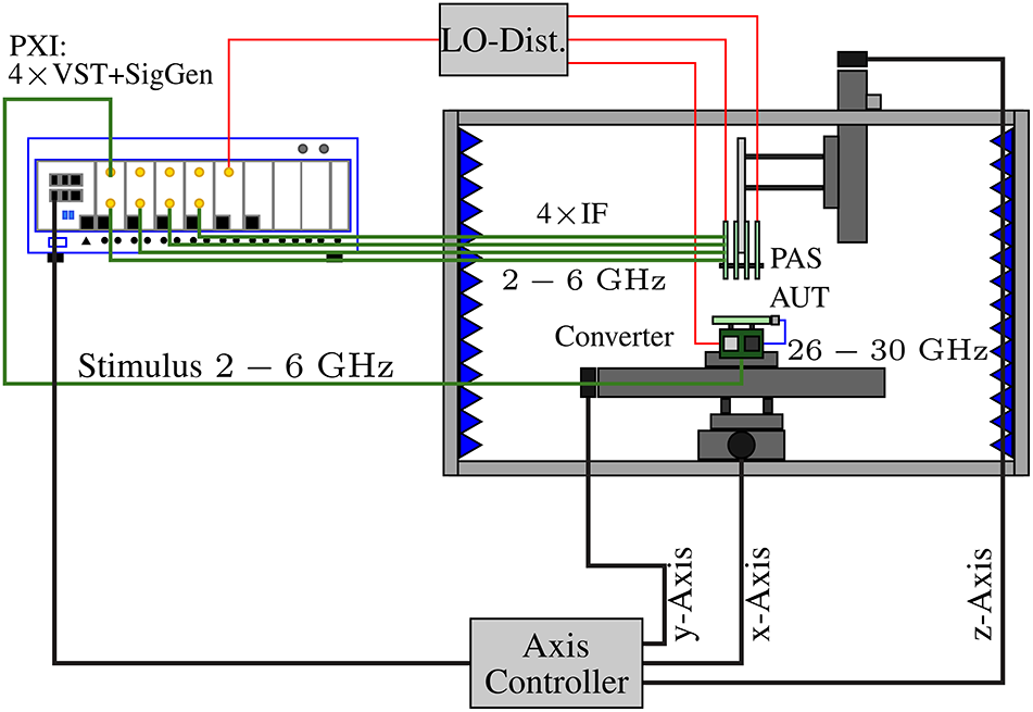
The diagram shown in Fig. 2 illustrates the multi-probe NF scanner setup used in this work. The NF scanner is constructed within a cage of extruded aluminum and uses three linear axes to position the antenna under test (AUT) and the active PAS relative to each other. The $x$- and $y$-axes span a planar scan area of $200\times200\,mm$. The $z$-axis has 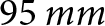$95\,mm$ of travel and allows to vary the $z$-distance between AUT and active PAS. In contrast to the general construction of planar NF scanners, we have chosen to move the AUT rather than the probe array. This decision was motivated by the number of radio frequency (RF) connections to the active PAS and their routing. This approach is feasible, since in comparison to a spherical or cylindrical scan setup, a planar scan setup only changes the absolute distance between AUT and probe and not the orientation. The movement of probe and AUT are therefore algorithmically interchangeable. The cage and surfaces inside of the scanner are lined with absorber materials to minimize the contributions of reflections to the NF scan. The multi-probe NF scanner measurement system uses a PCI eXtensions for Instrumentation system with four Vector Signal Transceivers (VSTs) to generate a stimulus for the AUT, the local oscillator (LO) for the active PAS and the converter printed circuit board (PCB) as well as capturing data from the probes. The VSTs are able to produce and process modulated signals from 2 to 6 GHz with 1 GHz bandwidth. These intermediate frequencies (IFs) are mixed with the common LO on a converter PCB, shown in Fig. 3, to the desired 26–30 GHz. The active PAS converts the mmWave signals back to the 2–6 GHz band. The converter PCB and active PAS are using identical converter architectures. The lower IF limits the effects of phase drifts and cable losses during the scan, while still enabling broadband measurements with the VSTs.

Figure 2.

Overview of the multi-probe NF scanner.

Figure 2 Long description

A multi-probe near-field scanner setup is illustrated. On the left, a PXI system labeled ′4 times VST plus SigGen′ is connected via red lines to an LO-Distribution box at the top. Green lines extend from the PXI to a section labeled ′Stimulus 2 to 6 GHz′ and ′4 times IF′. These lines lead into a rectangular enclosure on the right, which houses the PAS and AUT components. Inside this enclosure, the PAS and AUT are connected to a converter labeled ′2 to 6 GHz′ and ′26 to 30 GHz′. The enclosure is lined with blue zigzag patterns, possibly indicating absorber materials. Below the enclosure, an axis controller is connected to the x-axis, y-axis and z-axis, which are labeled with arrows indicating their directions. The x-axis and y-axis are shown as horizontal and vertical lines, respectively, while the z-axis is depicted as a vertical line with an arrow pointing upwards. The connections and components are arranged to demonstrate the flow and interaction between the PXI system, LO-Distribution and the scanner′s axes and components.

Figure 3.

Frequency converter PCB operating at 26–30 GHz (RF), 2–6 GHz (IF), and an LO of 6 GHz.

Probe array

Figure 4 shows the active PAS in detail. The active PAS currently supports up to 16 NF probe channels, which are able to operate between 26 and 30 GHz. The detailed construction and design choices of the active PAS are described and discussed in [Reference Obermaier, Laabs, Deckert and Plettemeier1]. Due to the limited number of IF channels on the VST system, we utilize only 4 of the 16 NF probes, and the active PAS provides to capture the NF of the AUT in this work. To maximize the scan area, we have chosen the four outermost corner elements of the probe array. The number of probes could be increased by utilizing an RF switch-matrix without the need of additional IF channels. Additionally, since the PAS is currently only able to measure a single polarization component at a time during a NF scan, we need to rotate the AUT by $90^{\circ}$ to capture co- and cross-polarization components of the AUT.

Figure 4.

Active PAS, with 16 NF probes (4 $\times$4 layout).

The NF measurement setup shown in this work should only be seen as an exemplary implementation of a planar multi-probe NF scanner. The principles and algorithms presented in this work can be transferred to other planar multi-probe scanners with similar constructions. There is also no need for a frequency conversion step or interchanging the movement of AUT and probes. We chose to reuse the ESA and active PAS in this work out of pragmatisms and our overall goal to expand the capabilities of the active PAS and the stationary NF to FF algorithms presented in [Reference Obermaier, Laabs, Deckert and Plettemeier1, Reference Obermaier, Lange, Deckert, Bossche and Plettemeier2].

NF processing

Figure 5 shows the NF amplitude and phase of a reference patch antenna captured by the four corner probes of the active PAS. The reference patch antenna fulfills multiple purposes during the NF processing steps. The main purpose of the reference patch antenna is to spatially align the captured NF samples in the $xy$-plane and correct for electrical offsets in the IF path of the active PAS. Furthermore, the reference patch antenna is also essential to perform the multi-probe compensation. Due to the construction of the active PAS, we cannot ensure the exact relative spatial offsets of each NF probe to the other probes in the array. But these relative spatial offsets can be reconstructed from the individual NF phase captures of each probe, given the knowledge that they are scanning the same AUT at the same $z$ distance. We are able to obtain these relative spatial offsets between the probes by calculating the phase center of the reference antenna in the $xy$-plane for each NF capture [Reference Obermaier, Deckert, Bossche and Plettemeier6]. This can be achieved by using a 2D phase unwrap algorithm and calculating a phase centroid for a given iso-phase [Reference Herráez, Burton, Lalor and Gdeisat8]. The antenna used during these measurements needs be well behaved in its phase pattern (e.g. radially symmetrical and without phase jumps, which are caused by side lobes) to not introduce errors during the unwrapping.

Figure 5.

NF capture of the main polarization of the reference antenna at 28 GHz. (A) Amplitude probe 1. (B) Phase probe 1. (C) Amplitude probe 2. (D) Phase probe 2. (E) Amplitude probe 3. (F) Phase probe 3. (G) Amplitude probe 4. (H) Phase probe 4.

Figure 5 Long description

Eight heatmaps capturing the near-field amplitude and phase of a reference antenna at 28 GHz using four probes. Each heatmap has x and y axes labeled in millimeters, ranging from minus 100 to 100. Amplitude heatmaps (A, C, E, G) display amplitude in decibel, with peaks at the center near 0 decibel. Phase heatmaps (B, D, F, H) show phase in degrees, with concentric rings indicating phase wrapping. Probe1 (A, B) shows a symmetrical amplitude peak and clear phase rings. Probe2 (C, D) displays similar amplitude but slightly distorted phase rings. Probe3 (E, F) has a broader amplitude spread and phase discontinuities. Probe4 (G, H) shows consistent amplitude with minor artifacts in phase rings. The comparison highlights differences in symmetry, peak location and phase behavior across probes.

Figure 6 shows the 2D unwrapped phase of probe 1 along the $xy$-plane, scanning the NF of the reference antenna. The shape highlighted by its white boundary is defined by an iso-phase of $\text{unwrap}(\arg(p1)) =\pi$. It is now possible to determine the relative offset of each probe and the origin, which is shown by the white cross, by calculating the centroid of this shape using every sample point $(x_i,y_i)$ inside the shape [Reference Protter and Morrey9].

Figure 6.

Unwrapped phase of NF probe 1 scanning the reference patch antenna.

(1)\begin{equation} x_0 = \frac{1}{N}\sum\limits_{i=0}^{N-1} x_i \end{equation}

(2)\begin{equation} y_0 = \frac{1}{N}\sum\limits_{i=0}^{N-1} y_i \end{equation}

To increase accuracy, the calculation can be repeated for multiple iso-phase values, e.g. $1.5\pi$, $2\pi$, and $3\pi$, and the result can be averaged. Based on the position of the phase centers 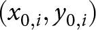$(x_{0,i},y_{0,i})$ in each NF capture, we are able to calculate a complex IF correction factor for each RF channel of the active PAS, which includes the probe and corresponding conversion channel. This complex correction factor is necessary, since each channel of the active PAS has a different electric length and, therefore, introduces a phase and amplitude offset. We denote these corrected NF captures as:

(3)\begin{equation} \begin{aligned} w_{1,cor}(x,y,z=z_0)& = w_{1}\\ w_{2,cor}(x,y,z=z_0)& = w_{2}\cdot\frac{w_2(x_{0,2},y_{0,2})}{w_1(x_{0,1},y_{0,1})}\\ w_{3,cor}(x,y,z=z_0)& = w_{3}\cdot\frac{w_3(x_{0,3},y_{0,3})}{w_1(x_{0,1},y_{0,1})}\\ w_{4,cor}(x,y,z=z_0)& = w_{4}\cdot\frac{w_4(x_{0,4},y_{0,4})}{w_1(x_{0,1},y_{0,1})} \end{aligned} \end{equation}

The raw samples $w_{i}(x,y,z=z_0)$ of main polarization are sampled at a distance $z_0$ and the coordinate 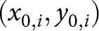$(x_{0,i},y_{0,i})$ is the location of the phase center in each capture. In an actual implementation of this approach, we would average the samples around this point to calculate the correction factor. The correction factors for the second polarization are identical, since we only rotate the AUT for this measurement and the IF and conversion path is not changed. Based on the calculated offset location 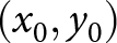$(x_0,y_0)$ of the phase center in each NF capture, it is now possible to superpose the four corrected NF captures. The superposed NF is shown in Fig. 7. In areas where the NF captures of the different probes overlap, the samples are averaged.

The combined NF can now be processed and transformed into the modal space as described in [Reference Obermaier, Deckert, Bossche and Plettemeier6]. This also includes an alignment of the combined NF phase center with the origin and windowing of the combined NF. The processed and transformed NF can then be expressed using planar modes as:

(4)\begin{equation} \begin{aligned} E_{x}(x,y,z_0)& = \iint\limits_{k_x,k_y}f_x(k_x,k_y) e^{-j(k_xx+k_yy+k_zz_0)}\mathrm{d}k_x \mathrm{d}k_y\\ E_{y}(x,y,z_0)& = \iint\limits_{k_x,k_y}f_y(k_x,k_y) e^{-j(k_xx+k_yy+k_zz_0)}\mathrm{d}k_x \mathrm{d}k_y \end{aligned} \end{equation}

The $z$-component of the wave vector is defined as 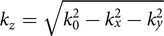$k_z = \sqrt{k_0^2-k_x^2-k_y^2}$ and $k_0$ is the wavenumber in vacuum. $E_{x,y}$ are the combined and processed NF samples shown in Fig. 7. Figure 8 shows the modal spectrum of the combined and processed NF. The modal spectrum has been corrected for the measurement distance $z_0$ by holographic correction [Reference Obermaier, Deckert, Bossche and Plettemeier6].

Figure 7.

Combined NF samples of the reference antenna (primary polarization) at 28 GHz.

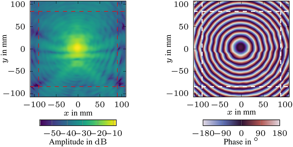
Figure 7 Long description

Near-field amplitude distribution at 28 GHz: The x-axis ranges from minus 100 to 100 millimeters and the y-axis ranges from minus 100 to 100 millimeters. The color scale represents amplitude in decibels, ranging from minus 50 to 0. A central peak is visible near x equals 0 and y equals 0, indicating a high amplitude region. Near-field phase distribution at 28 GHz: The x-axis ranges from minus 100 to 100 millimeters and the y-axis ranges from minus 100 to 100 millimeters. The color scale represents phase in degrees, ranging from minus 180 to 180. Multiple concentric rings are centered near x equals 0 and y equals 0, indicating phase variation. The amplitude map shows a concentrated energy region, while the phase map reveals symmetrical phase shifts.

Figure 8.

Modal spectrum of the reference antenna 28 GHz with no probe correction (main polarization).

Figure 8 Long description

Two heatmaps illustrate the modal spectrum of a reference antenna at 28 GHz without probe correction. The left heatmap represents amplitude in decibels, with the x-axis labeled k subscript x over k subscript 0 and the y-axis labeled k subscript y over k subscript 0, both ranging from minus 1.5 to 1.5. The color scale ranges from 135 to 105 decibels, showing a smooth circular field. The right heatmap depicts phase in degrees, with the same axis labels and ranges. The color scale ranges from minus 180 to 180 degrees, highlighting strong variation near the boundary. The left panel shows a bulk-uniform field, while the right panel reveals boundary-localized variation. The key takeaway is the contrast between amplitude and phase distribution across the modal spectrum.

Multi-probe correction

To reconstruct the correct FF from the measured modal spectrum shown in Fig. 8, it is necessary to correct the modal spectrum for the influence of the probes used to sample the NF. Every real probe shows directivity, which attenuates some of the measured AUT modes and may also change their phase. To incorporate the effect of probe directivity, Equation 4 has to be rewritten as:

(5)\begin{equation} \begin{aligned} \mathbf{E}(x,y,z)& = \iint\limits_{k_x,k_y}\mathbf{f}_{P}(\mathbf{k})\cdot \mathbf{f}_{AUT}(\mathbf{k}) e^{-j(\mathbf{k}\mathbf{r})}\mathrm{d}k_{x,y} \end{aligned} \end{equation}

(6)\begin{equation} \begin{aligned} \mathbf{f}_{P}(k_x,k_y)& = \begin{bmatrix} f_{pp1}(k_x,k_y) & f_{cp1}(k_x,k_y)\\ f_{cp2}(k_x,k_y) & f_{pp2}(k_x,k_y) \end{bmatrix} \end{aligned} \end{equation}

The modal spectra $f_{pp1,2}$ and $f_{cp1,2}$ are the principle and cross-polarization responses of the probe in the modal spectrum. Since we assume that the same probes measure both principle and cross-polarization responses, we know that $f_{pp1}(\phi) = f_{pp2}(\phi+90^{\circ})$ and $f_{cp1}(\phi) = f_{cp2}(\phi+90^{\circ})$ [Reference Masters10]. The modal spectrum 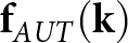$\mathbf{f}_{AUT}(\mathbf{k})$ describes the true modal spectrum of the AUT. In the case of a single probe, 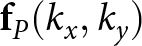$\mathbf{f}_{P}(k_x,k_y)$ can be easily calculated from the probe pattern or derived analytically for special probes [Reference Gregson, McCormick and Parini11]. This approach is not feasible for a multi-probe NF scanner, since coupling and shading effects cannot be neglected inside the probe array, due to the close proximity of the probes. We are also not able to measure the probe response a classical FF setup due to the construction of the probe array. Instead of determining the probe response of every probe in the array, we will characterize the overall response of the complete probe array using a known reference antenna. Since we have measured the true FF of the reference antenna shown in Fig. 9, we are able to calculate the equivalent modal spectrum of the reference antenna. This, in turn, allows us to compute the multi-probe response, which has been defined in Equation 6, from the FF and NF measurements of the reference antenna similar to the approach presented in [Reference Masters10]. The stationary phase approximation allows the approximation of the FF based on the modal spectrum [Reference Balanis12]:

Figure 9.

Reference antenna pattern designed for 26–30 GHz.

Figure 9 Long description

The polar plot illustrates antenna radiation patterns measured at 28 gigahertz. The angular axis is labeled in degrees, ranging from 0 to 90 degrees on both sides. The radial axis represents gain in decibels, with values marked at minus 10, minus 20 and minus 30. Four series are plotted: Measured V Cut at 28 gigahertz co polarization as a solid line, Measured H Cut at 28 gigahertz co polarization as a dashed line, Measured V Cut at 28 gigahertz cross polarization as a solid line and Measured H Cut at 28 gigahertz cross polarization as a dashed line. The co polarization patterns show stronger main lobes compared to cross polarization, with notable nulls in cross polarization. The V Cut co polarization exhibits higher peaks than the H Cut. The board above the plot serves as the antenna fixture, designed for 26 to 30 gigahertz, with a central metal trace and circular holes for mounting.

(7)\begin{equation} \begin{aligned} E_\theta(r,\theta,\phi)&\simeq j\frac{k\cdot e^{-jkr}}{2\pi r} \left( f_x \cos(\phi)+f_y\sin(\phi) \right)\\ E_\phi(r,\theta,\phi)&\simeq j\frac{k\cdot e^{-jkr}}{2\pi r} \cos(\theta) \left( -f_x \cos(\phi)+f_y\sin(\phi) \right) \end{aligned} \end{equation}

Based on Equation 7, we are able to calculate the modal spectrum of the reference antenna by:

(8)\begin{equation} \begin{aligned} f_x &= \frac{E_\theta\cos(\phi) - E_\phi\sin(\phi) }{\cos(\theta)}\\ f_y &= \frac{E_\theta\sin(\phi) + E_\phi\cos(\phi) }{\cos(\theta)} \end{aligned} \end{equation}

Since there exists a singularity at 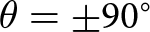$\theta = \pm 90^{\circ}$, it is necessary to limit the spectrum to a value 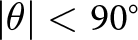$|\theta| \lt 90^{\circ}$. A sensible choice for this limit of $\theta$ is the truncation angle $\theta_v$, which is inherent to planar NF scanners and dependent on the dimensions of the scanning plane and scanning distance between AUT and probe [Reference Newell3].

Given the measured NF 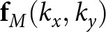$\mathbf{f}_{M}(k_x,k_y)$ composed of all probes as well as the true spectrum 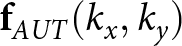$\mathbf{f}_{AUT}(k_x,k_y)$ derived from the FF measurement, we are able to calculate the probe response 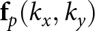$\mathbf{f}_{p}(k_x,k_y)$. Using Equations 5 and 6, we can express the relation between 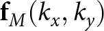$\mathbf{f}_{M}(k_x,k_y)$ and 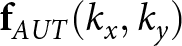$\mathbf{f}_{AUT}(k_x,k_y)$ as:

(9)\begin{equation} \begin{aligned} f_{M,x}(k_x,k_y)& = f_{pp1}(k_x,k_y)\cdot f_{AUT,x}(k_x,k_y)\\ &+f_{cp1}(k_x,k_y)\cdot f_{AUT,y}(k_x,k_y)\\ f_{M,y}(k_x,k_y)& = f_{cp2}(k_x,k_y)\cdot f_{AUT,x}(k_x,k_y)\\ & +f_{pp2}(k_x,k_y)\cdot f_{AUT,y}(k_x,k_y) \end{aligned} \end{equation}

Equation 9 is underdetermined with four unknowns and two equations, but since $f_{pp1}(\phi) = f_{pp2}(\phi+90^{\circ})$ and $f_{cp1}(\phi) = f_{cp2}(\phi+90^{\circ})$ it follows that:

(10)\begin{equation} \begin{aligned} f_{pp,2}(k_x,k_y)& = f_{pp,1}(-k_y,k_x)\\ f_{cp,2}(k_x,k_y)& = f_{cp,1}(-k_y,k_x) \end{aligned} \end{equation}

This allows us to substitute the second equation of Equation 9 by calculating the point 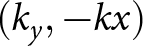$(k_y,-kx)$ and using the properties described in Equation 10. This results in two equations for two unknowns, which allow us to solve for all 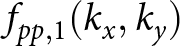$f_{pp,1}(k_x,k_y)$ and 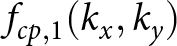$f_{cp,1}(k_x,k_y)$. And 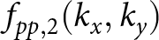$f_{pp,2}(k_x,k_y)$ as well as 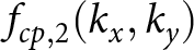$f_{cp,2}(k_x,k_y)$ can be found by applying Equation 10.

(11)\begin{equation} \begin{aligned} f_{M,x}(k_x,k_y)& = f_{pp1}(k_x,k_y)\cdot f_{AUT,x}(k_x,k_y)\\ &+f_{cp1}(k_x,k_y)\cdot f_{AUT,y}(k_x,k_y)\\ f_{M,y}(k_y,-k_x)&=f_{cp2}(k_y,-k_x)\cdot f_{AUT,x}(k_y,-k_x)\\ &+f_{pp2}(k_y,-k_x)\cdot f_{AUT,y}(k_y,-k_x)\\ f_{M,y}(k_y,-k_x)&=f_{cp1}(k_x,k_y)\cdot f_{AUT,x}(k_y,-k_x)\\ &+f_{pp1}(k_x,k_y)\cdot f_{AUT,y}(k_y,-k_x) \end{aligned} \end{equation}

The overall probe effect for the principle polarization 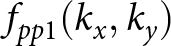$f_{pp1}(k_x,k_y)$ at 28 GHz is shown in Fig. 10 and can now be applied to the captured NF of any scanned AUT.

Figure 10.

Modal correction spectrum at 28 GHz.

Measurement results

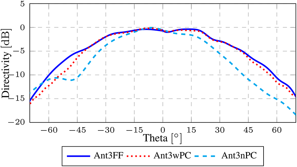
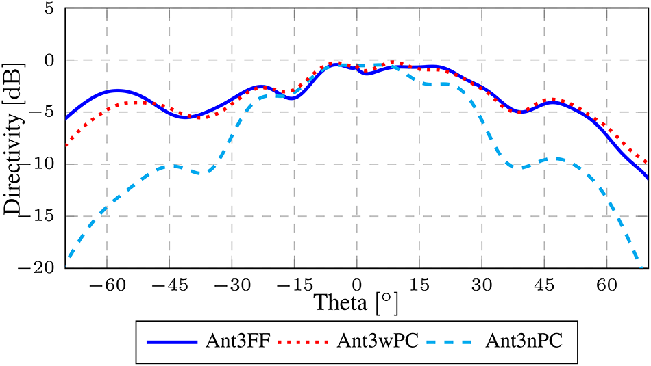
To validate our approach, we measured a $4\times 4$ ESA antenna, which is shown in Fig. 1 and operates between 26 and 30 GHz, with the multi-probe NF scanning system as well as with a conventional spherical FF scanner. The ESA is identical to the one used in [Reference Obermaier, Laabs, Deckert and Plettemeier1, Reference Obermaier, Lange, Deckert, Bossche and Plettemeier2] and [Reference Obermaier, Deckert, Bossche and Plettemeier6]. During the measurement only a single element of the ESA was active at a time. Figures 11 and 12 show the FF pattern cut, measured by a spherical scanner (FF), as well as the reconstructed FF from the multi-probe NF scanner with and without probe correction applied to the captured NF for antenna element 3 of the ESA. The figure shows that the reconstructed FF pattern agrees very well with the measured FF pattern up to the angle of validity, which was 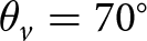$\theta_v=70^{\circ}$ for this measurement setup. In principle, the scanner could measure a fully active array, but the limited $xy$-travel would limit the angle of validity to below 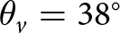$\theta_v=38^{\circ}$ at the necessary measurement distance outside the reactive NF of the fully active ESA.

Figure 11.

Comparison of measured FF, reconstructed FF with and without probe correction of antenna element 3 at 28 GHz (H-Cut).

Figure 12.

Comparison of measured FF, reconstructed FF with and without probe correction of antenna element 3 at 28 GHz (V-Cut).