2 Physical model and numerical methods

In this paper, we consider the flow in a differentially heated parallelepipedic cavity of aspect ratios $A_{X}=L/h=4$ and $A_{Y}=l/h=2$ , where $L$ is the length along the longitudinal $x$ -direction, $l$ is the width along the transverse $y$ -direction and $h$ is the height along the vertical $z$ -direction (see figure 1, where the main middle vertical planes, either the longitudinal $V_{l}$ plane or the transverse $V_{t}$ plane, are presented). The vertical end walls are isothermal and held at different temperatures, $T_{H}$ at the right hot end wall and $T_{C}$ at the left cold end wall, and the side walls are insulating. The fluid is assumed to be Newtonian with constant physical properties (kinematic viscosity $\unicode[STIX]{x1D708}$ , thermal diffusivity  $\unicode[STIX]{x1D705}$ , density  $\unicode[STIX]{x1D70C}$ ), except for the density in the buoyancy term, which, in the Boussinesq approximation, depends linearly on the temperature, $\unicode[STIX]{x1D70C}=\unicode[STIX]{x1D70C}_{0}(1-\unicode[STIX]{x1D6FD}(T-T_{0}))$ , where $\unicode[STIX]{x1D6FD}$ is the thermal expansion coefficient, $T_{0}=(T_{C}+T_{H})/2$ is a reference temperature, and $\unicode[STIX]{x1D70C}_{0}$ is the value of the density at  $T_{0}$ .

Figure 1.

Geometry of the differentially heated cavity. The end walls located at $\bar{x}=-L/2$ and $\bar{x}=L/2$ are held at fixed temperatures $T_{C}$ and $T_{H}$ (with $T_{H}>T_{C}$ ), respectively, whereas the side walls are insulating boundaries.

The convective motion in the differentially heated cavity is governed by the momentum, mass and energy conservation equations. By using  $h$ , $h^{2}/\unicode[STIX]{x1D708}$ , $\unicode[STIX]{x1D708}/h$ , $\unicode[STIX]{x1D70C}_{0}\unicode[STIX]{x1D708}^{2}/h^{2}$ and $\unicode[STIX]{x0394}T/A_{X}$ $(\unicode[STIX]{x0394}T=T_{H}-T_{C})$ as reference quantities for length, time, velocity, pressure and temperature, respectively, the equations take the following dimensionless form:

(2.1) $$\begin{eqnarray}\displaystyle & \displaystyle \frac{\unicode[STIX]{x2202}\boldsymbol{v}}{\unicode[STIX]{x2202}t}+\boldsymbol{v}\boldsymbol{\cdot }\unicode[STIX]{x1D735}\boldsymbol{v}=-\unicode[STIX]{x1D735}p+\unicode[STIX]{x1D6FB}^{2}\boldsymbol{v}+Gr\,\unicode[STIX]{x1D6E9}\boldsymbol{e}_{z}, & \displaystyle\end{eqnarray}$$

(2.2) $$\begin{eqnarray}\displaystyle & \displaystyle \frac{\unicode[STIX]{x2202}\unicode[STIX]{x1D6E9}}{\unicode[STIX]{x2202}t}+\boldsymbol{v}\boldsymbol{\cdot }\unicode[STIX]{x1D735}\unicode[STIX]{x1D6E9}=\frac{1}{Pr}\unicode[STIX]{x1D6FB}^{2}\unicode[STIX]{x1D6E9}, & \displaystyle\end{eqnarray}$$

(2.3) $$\begin{eqnarray}\displaystyle & \unicode[STIX]{x1D735}\boldsymbol{\cdot }\boldsymbol{v}=0, & \displaystyle\end{eqnarray}$$

where $Gr=g\unicode[STIX]{x1D6FD}h^{3}\unicode[STIX]{x0394}T/(A_{X}\unicode[STIX]{x1D708}^{2})$ is the Grashof number, $Pr=\unicode[STIX]{x1D708}/\unicode[STIX]{x1D705}$ is the Prandtl number and $\unicode[STIX]{x1D6E9}=(T-T_{0})A_{X}/\unicode[STIX]{x0394}T$ is a reduced temperature. Note that the origin of the coordinates is taken at the centre $C$ of the cavity.

The boundary conditions are $\boldsymbol{v}=0$ (no-slip conditions) for the velocity on all the boundaries, $(\unicode[STIX]{x2202}\unicode[STIX]{x1D6E9}/\unicode[STIX]{x2202}z)(z=\pm 1/2)=0$ and $(\unicode[STIX]{x2202}\unicode[STIX]{x1D6E9}/\unicode[STIX]{x2202}y)(y=\pm A_{Y}/2)=0$ for the temperature on the insulating side walls, and $\unicode[STIX]{x1D6E9}(x=\pm A_{X}/2)=\pm A_{X}/2$ for the temperature on the isothermal end walls.

Equations (2.1), (2.2) and (2.3) are solved in the three-dimensional domain using a spectral element code developed by Ben Hadid & Henry (Reference Ben Hadid and Henry1997). This code is based on a spatial discretization using the Gauss–Lobatto–Legendre polynomials. The time discretization is carried out by a semi-implicit scheme proposed by Karniadakis (Reference Karniadakis1991), where the nonlinear terms are included explicitly, the pressure is then obtained from a derived pressure equation enforcing the incompressibility constraint (with consistent boundary conditions) and finally the linear terms are integrated implicitly.

The time integration scheme is used with the third-order-accurate formulation proposed by Karniadakis (Reference Karniadakis1991) for transient computations or unsteady flow simulations. It is also used in its first-order formulation to compute steady state solutions, eigenvalues and eigenvectors determining their stability, and bifurcation points. All these computations are based on a Newton–Krylov method and follow the ideas of Mamun & Tuckerman (Reference Mamun and Tuckerman1995) and Bergeon et al. (Reference Bergeon, Henry, Ben Hadid and Tuckerman1998). They are integrated in a continuation algorithm and, complemented by an Arnoldi method, they allow us to obtain bifurcation diagrams of the steady flow solutions. These methods will not be described further here as they have been already presented and well discussed by Henry & Ben Hadid (Reference Henry and Ben Hadid2007) and Torres et al. (Reference Torres, Henry, Komiya, Maruyama and Ben Hadid2013, Reference Torres, Henry, Komiya and Maruyama2014). In these papers, the methods were successfully used in different problems of buoyant convection.

The continuation of periodic orbits (or cycles) has also been developed more recently using the method proposed by Sánchez et al. (Reference Sánchez, Net, García-Archilla and Simó2004) and successfully used by Puigjaner et al. (Reference Puigjaner, Herrero, Simó and Giralt2011) in a Rayleigh–Bénard problem. The novelty here is that the method is developed from a time integration scheme using time splitting. The method is based on a Newton–Krylov approach in which the periodic states of (2.1)–(2.3) are obtained as fixed points of a Poincaré map. In our code, the hyperplane defining the Poincaré map corresponds to a given value $k_{p}$ for  $u^{\ast }$ , the longitudinal velocity at a chosen point inside the cavity, i.e. $u^{\ast }=k_{p}$ . The trajectories in the phase space used to approach the periodic state are computed with the time integration scheme at third order with a time step $\unicode[STIX]{x0394}t_{c}=5\times 10^{-5}$ . These trajectories are initiated from a point in the Poincaré hyperplane using two first-order time steps with $\unicode[STIX]{x0394}t=\unicode[STIX]{x0394}t_{c}/4$ and three second-order time steps with $\unicode[STIX]{x0394}t=\unicode[STIX]{x0394}t_{c}/2$ , until third-order time steps with $\unicode[STIX]{x0394}t=\unicode[STIX]{x0394}t_{c}$ can be applied. The exact return of the trajectory to the Poincaré hyperplane is obtained by a Newton–Krylov approach as proposed by Sánchez et al. (Reference Sánchez, Net, García-Archilla and Simó2004). Finally, the successive corrections of the initial point in the Poincaré hyperplane, necessary to converge to a closed loop (the expected cycle), are obtained, as indicated above, by Newton–Krylov steps. As shown by Sánchez et al. (Reference Sánchez, Net, García-Archilla and Simó2004), at each Newton–Krylov step, the linear system giving the correction can be solved by GMRES (generalized minimal residual method) iterations, where the matrix–vector products correspond to the evolution of a perturbation obtained by iterating the linearized version of (2.1)–(2.3) along the last calculated trajectory in the phase space. The correction thus obtained at a Newton–Krylov step is eventually adapted to lie in the Poincaré hyperplane. The convergence to the periodic solution is assumed to be obtained when the mean square difference between the initial and end points in the Poincaré hyperplane is less than  $10^{-6}$ . The method was found to work well with a convergence generally obtained with a few Newton–Krylov steps (2–4), each Newton–Krylov step requiring 5–15 GMRES iterations for a prescribed precision of  $10^{-2}$ .

The stability of these periodic solutions is investigated in the framework of the Floquet theory (Klausmeier Reference Klausmeier2008; Seydel Reference Seydel2010). We use an Arnoldi method in which the Arnoldi basis is obtained by repeating the same process as for the GMRES iterations, i.e. computing the evolution of a perturbation by iterating the linearized version of (2.1)–(2.3) along the considered periodic solution. The complex eigenvalues $\unicode[STIX]{x1D70E}$ obtained by the Arnoldi method are the Floquet multipliers. If the norm of $\unicode[STIX]{x1D70E}$ is smaller (larger) than 1, i.e. the Floquet multiplier is inside (outside) the unit circle, the perturbation associated with the corresponding eigenvector will decrease (increase) during the cycle, indicating a stabilizing (destabilizing) behaviour. Note, however, that there is always a Floquet multiplier equal to $(+1)$ , corresponding to a perturbation exactly along the cycle, which will neither decrease nor increase. Excluding this last eigenvalue, the periodic solution will be unstable if there is at least one Floquet multiplier outside the unit circle (i.e. $\exists j$ , $|\unicode[STIX]{x1D70E}_{j}|>1$ ). Conversely, if all the Floquet multipliers are inside the unit circle (i.e. $\forall j$ , $|\unicode[STIX]{x1D70E}_{j}|<1$ ), the periodic solution is stable. Finally, depending on how these Floquet multipliers cross the unit circle, three kinds of bifurcation can be obtained. If the unstable Floquet multiplier is real, a period-doubling bifurcation will occur for $\unicode[STIX]{x1D70E}=-1$ and a bifurcation toward another limit cycle with the same frequency for $\unicode[STIX]{x1D70E}=+1$ . In contrast, if the unstable Floquet multiplier is a pair of complex conjugate eigenvalues, a Naimark–Sacker bifurcation (also called the generalized Hopf bifurcation) toward a quasi-periodic solution is identified. In practice, the ten leading Floquet multipliers were calculated with the Arnoldi method and the precise convergence ( $10^{-10}$ ) was obtained within a limited number of Arnoldi steps (50–60).

The refined grid used for all our calculations of convective flow in a cavity with aspect ratios $A_{X}=4$ and $A_{Y}=2$ has $47\times 37\times 27$ points in the  $x$ , $y$ and $z$ directions, respectively. As shown in table 1 for some examples, this grid gives excellent resolution of the thresholds $Gr_{c}$ of the different bifurcation points, indicating that both the solution and the eigenvector that will induce the oscillatory behaviour are well resolved on the grid.

Table 1.

Mesh refinement tests of numerical accuracy of the critical Grashof number $Gr_{c}$ for different flow bifurcations detected in a laterally heated cavity ( $A_{X}=4$ , $A_{Y}=2$ , $Pr=0.005$ ): steady bifurcation $P_{l}^{P}$ and Hopf bifurcation $H_{a}^{P}$ for which the value of $\unicode[STIX]{x1D714}_{c}$ is also given.

3 Steady flow at low Grashof numbers

In our differentially heated parallelepipedic cavity, a convective flow will appear as soon as the Grashof number $Gr$ is not zero. At low  $Gr$ , this flow is steady, unicellular and occupies the whole enclosure. More precisely, the fluid rises at the hot wall, travels longitudinally throughout the cavity and goes down at the cold wall, before returning to the hot wall (figure 2). As long as the temperature field remains diffusive and the inertial effects remain small (approximately up to $Gr=1000$ ), the flow structure is invariant, with in particular a quasi-parallel flow in the core of the cavity (Hadley flow, see Hart (Reference Hart1972)), and only its intensity varies linearly with  $Gr$ . In the Boussinesq approximation, this steady flow exhibits different symmetries coming from the symmetries of the equations, the geometry and the boundary conditions:

1. (i) a reflection symmetry $S_{l}$ with respect to the middle vertical $V_{l}$ plane ( $y=0$ ), also called left/right symmetry:

   (3.1) $$\begin{eqnarray}S_{l}:(x,y,z,t)\rightarrow (x,-y,z,t),\quad (u,v,w,\unicode[STIX]{x1D6E9})\rightarrow (u,-v,w,\unicode[STIX]{x1D6E9}),\end{eqnarray}$$

2. (ii) a $\unicode[STIX]{x03C0}$ -rotational symmetry $S_{\unicode[STIX]{x03C0}}$ with respect to the central transverse $y$ -axis ( $x=0$ , $z=0$ ):

   (3.2) $$\begin{eqnarray}S_{\unicode[STIX]{x03C0}}:(x,y,z,t)\rightarrow (-x,y,-z,t),\quad (u,v,w,\unicode[STIX]{x1D6E9})\rightarrow (-u,v,-w,-\unicode[STIX]{x1D6E9}),\end{eqnarray}$$

3. (iii) a symmetry $S_{c}$ with respect to the centre $C$ of the cavity, which is such that:

   (3.3) $$\begin{eqnarray}S_{c}=S_{\unicode[STIX]{x03C0}}.S_{l}.\end{eqnarray}$$

These symmetries belong to a $Z_{2}\times Z_{2}=D_{2}$ group, which contains four elements (including the identity  $I$ ). Note that we will also use the notations $S_{a}$ and $S_{w}$ for flows with all the symmetries and without symmetry, respectively.

Figure 2.

For $Pr=0.025$ and $Gr=3\times 10^{4}$ : (a) longitudinal velocity field $u(y,z)$ in the $V_{t}$ plane; (b) velocity vector ( $\boldsymbol{u},\boldsymbol{w}$ ) and temperature $-2\leqslant \unicode[STIX]{x1D6E9}(x,z)\leqslant 2$ fields in the $V_{l}$ plane; (c) a three-dimensional visualization of the velocity vector field showing the circulation loop in the cavity.

The plot of the longitudinal velocity component in the transverse $V_{t}$ plane, $u(y,z)$ , given in figure 2(a) allows to clearly visualize these symmetries. Indeed, for $u$ in this plane, the $S_{\unicode[STIX]{x03C0}}$ symmetry is expressed by $(y,z)\rightarrow (y,-z)$ , $u\rightarrow -u$ , the $S_{l}$ symmetry is given by $(y,z)\rightarrow (-y,z)$ , $u\rightarrow u$ and finally, the $S_{c}$ symmetry is such that $(y,z)\rightarrow (-y,-z)$ , $u\rightarrow -u$ . Such a plot can then be used to see the symmetries of solutions on new branches appearing at bifurcation points. Applied on a critical eigenvector $u^{\prime }(y,z)$ (figure 5), the plot will also indicate which symmetries are kept or broken (in that case, they appear as anti-symmetries) at the corresponding bifurcation point.

The changes which affect the steady three-dimensional flow structure (shown in figure 2 before any symmetry breaking at bifurcations) when the Grashof number is increased are described in Henry & Buffat (Reference Henry and Buffat1998) and Henry & Ben Hadid (Reference Henry and Ben Hadid2007). At $Gr=10\,000$ , the uni-cellular flow appears to be already tilted compared to the parallel Hadley circulation. For larger values of $Gr$ , the uni-cellular flow evolves towards a centred roll-like structure inside a remaining long-scale circulation. As indicated by Henry & Buffat (Reference Henry and Buffat1998), these changes are the sign of an imperfect bifurcation which is connected with the steady transition towards transverse rolls (shear instability) found in the stability analysis of the parallel Hadley flow (Hart Reference Hart1972). At sufficiently high values of the Grashof number, this basic steady flow will eventually be destabilized at different bifurcation points, which will trigger new steady or oscillatory flow solutions. This is discussed in the next sections.

4 Bifurcation analysis of the steady flows

In a previous work, Henry & Ben Hadid (Reference Henry and Ben Hadid2007) determined the threshold of the first instability of the basic steady flow in a differentially heated parallelepipedic cavity for a wide range of aspect ratios $A_{X}$ and $A_{Y}$ and Prandtl numbers. They showed the strong variation of these thresholds, which were associated with instabilities of different types (steady or oscillatory), breaking different symmetries. In the present study, the cavity dimensions are held constant ( $A_{X}=4$ and $A_{Y}=2$ ) and only the effect of the Prandtl number will then be depicted. However, we will not focus on the first instability of the basic steady flow, but more largely consider all the bifurcation points that could be involved in the further dynamics of the flow, on the basic steady flow branch (primary branch) as well as on the steady branches that bifurcate from it (secondary branches). Note that, in the different bifurcation diagrams presented in this study, we plot  $u^{\ast }$ , the normalized longitudinal velocity component ( $u/\sqrt{Gr}$ ) at a representative point in the cavity ( $x=0$ , $y=0.49391$ , $z=-0.36911$ ), as a function of $Gr$ . Finally, the stability of the branches (branches of steady states as well as branches of cycles) on these bifurcation diagrams is indicated through a couple of numbers $n-m$ where $n$ is the number of unstable real eigenvalues whereas $m$ is the number of unstable couples of complex conjugate eigenvalues. $0-0$ is thus the indication of a stable branch.

Figure 3.

Bifurcation diagram ( $u^{\ast }$ versus $Gr$ ) for $Pr=0.015$ showing all the bifurcation points in the range $3.0\times 10^{4}\leqslant Gr\leqslant 5.1\times 10^{4}$ . Stable steady solutions are represented by solid lines whereas dashed lines represent unstable steady solutions. The symmetry of these steady solutions ( $S_{a}$ for the leading branch and $S_{l}$ for the secondary branch) is shown in the insets. More information on the stability is given by the number of unstable eigenvalues $n-m$ indicated along the branches (see text).

Table 2.

Critical thresholds $Gr_{c}$ of the principal bifurcation points ( $P$ for pitchfork, $H$ for Hopf) on the primary (superscript  $P$ ) and secondary (superscript  $S$ ) branches for $Pr=0$ , 0.005, 0.015 and 0.025. The subscripts $c$ , $l$ , $\unicode[STIX]{x03C0}$ , $a$ and $w$ refer to the symmetries kept by the marginal mode at the bifurcation: symmetries $S_{c}$ , $S_{l}$ , $S_{\unicode[STIX]{x03C0}}$ , all the symmetries and without symmetry, respectively. In case of Hopf bifurcation points, the critical frequency at threshold $f_{c}$ is also given.

As a starting point, we have computed bifurcation diagrams of the steady flow solutions for several Prandtl numbers going from 0 to 0.025 (see figure 3 and the steady part of the different bifurcation diagrams in figures 6 a, 7 a, 8 a, 10 a). In all these cases, a single steady bifurcation point $P_{l}^{P}$ is found on the primary branch (see table 2). As shown in figure 3, this bifurcation is a supercritical pitchfork bifurcation which breaks the $S_{c}$ and $S_{\unicode[STIX]{x03C0}}$ symmetries and keeps the $S_{l}$ symmetry. The secondary branch initiated at this point thus corresponds to flow states with only the $S_{l}$ symmetry (see insets of figure 3 for example). Note that, as expected, two secondary branches appear at the pitchfork bifurcation. These branches are dynamically equivalent as the solution on one branch is the symmetric of the solution on the other branch by the broken $S_{c}$ or $S_{\unicode[STIX]{x03C0}}$ symmetry. For this reason, only one of these branches will often be considered and plotted. The principal bifurcation points on these steady primary and secondary branches are also determined. Except $P_{l}^{P}$ , they are all Hopf bifurcation points (see figure 3) and their critical characteristics (critical threshold $Gr_{c}$ and frequency  $f_{c}$ ) are given in table 2. In order to identify all the different bifurcation points, we have given them specific names depending on their properties. These points are either steady pitchfork ( $P$ ) or oscillatory ( $H$ for Hopf). The type of the branch (primary or secondary) on which they appear is indicated by a superscript ( $P$ for primary branch and $S$ for secondary branch), whereas the symmetry preserved by the critical mode at the bifurcation is denoted by a subscript. More precisely, the subscripts  $c$ , $l$ and $\unicode[STIX]{x03C0}$ correspond to the centro-symmetry  $S_{c}$ , the left/right symmetry $S_{l}$ and the $\unicode[STIX]{x03C0}$ -rotational symmetry  $S_{\unicode[STIX]{x03C0}}$ , respectively, whereas the subscript $a$ ( $w$ ) indicates critical modes with all the symmetries (without symmetry). For example, the points $H_{a}^{P}$ and $H_{l}^{S}$ are the Hopf bifurcation point on the primary branch for which all the symmetries are kept and the Hopf bifurcation point on the secondary branch that keeps only the $S_{l}$ symmetry, respectively. The same type of notations will be used later for the bifurcations occurring on cycles: the superscript $P$ or $S$ will be changed to $C$ to mention that the bifurcation occurs on a cycle, but with a further indication on the symmetry of the cycle. For example the superscript $C_{a}$ will indicate that the bifurcation occurs on a cycle with all the symmetries. The subscript will still indicate the symmetry preserved by the critical mode.

Figure 4.

Tracking of the main bifurcation points in the ( $Pr,Gr_{c}$ ) parameter space. (a) Global view in the range $0\leqslant Pr\leqslant 0.025$ . (b) Zoom of the region $Pr\leqslant 6\times 10^{-4}$ in order to highlight the crossing of the $P_{l}^{P}$ and $H_{c,0}^{P}$ primary bifurcation points at $Pr=8.83\times 10^{-5}$ with the creation of the $H_{w,0}^{S}$ secondary bifurcation at this co-dimension 2 point. (c) Zoom around the crossing of the $P_{l}^{P}$ and $H_{c,25}^{P}$ primary bifurcation points at $Pr=1.63\times 10^{-2}$ highlighting the creation of the $H_{w,25}^{S}$ secondary bifurcation at this other co-dimension 2 point. In this figure, squares are used for modes with $S_{l}$ (left–right) symmetry, circles for modes with $S_{c}$ (centre) symmetry, triangles for modes with $S_{\unicode[STIX]{x03C0}}$ ( $\unicode[STIX]{x03C0}$ -rotational) symmetry, diamonds for modes with all the symmetries and stars for modes without symmetry. The symbols are filled (empty) for primary (secondary) bifurcation points. The thresholds for  $P_{l}^{P}$ , the only steady bifurcation, are given as black squares.

Figure 5.

Contours of the longitudinal velocity perturbation $u^{\prime }(y,z)$ in the transverse $V_{t}$ plane for the critical modes (real part) associated with different bifurcation points: (a–f) correspond to $H_{c,25}^{P}$ at $Pr=0.025$ , $H_{w,25}^{S}$ at $Pr=0.015$ , $P_{l}^{P}$ , $H_{l}^{S}$ and $H_{a}^{P}$ at $Pr=0.005$ and finally $H_{c,0}^{P}$ at $Pr=0$ , respectively.

From figure 3 and table 2, we can see that five main modes were found on the primary steady branch ( $P_{l}^{P}$ , $H_{c,0}^{P}$ , $H_{c,25}^{P}$ , $H_{a}^{P}$ and $H_{\unicode[STIX]{x03C0}}^{P}$ ) and four other modes ( $H_{l}^{S}$ , $H_{w,0}^{S}$ , $H_{w,1}^{S}$ and $H_{w,25}^{S}$ ) on the secondary steady branch initiated at the steady point  $P_{l}^{P}$ . All these bifurcation points were then precisely tracked as a function of $Pr$ in the whole range $0\leqslant Pr\leqslant 0.025$ . The location of these points in the ( $Pr,Gr_{c}$ ) parameter space is shown in figure 4 and the plots of the corresponding critical modes in the transverse $V_{t}$ plane are given in figure 5. Note that, in some cases, we have introduced an index in the subscript in order to distinguish bifurcation points corresponding to modes with the same symmetry. The index 0 was chosen for the bifurcation $H_{c,0}^{P}$ which is the first to appear at $Pr=0$ and for the bifurcation $H_{w,0}^{S}$ issued from $H_{c,0}^{P}$ . Similarly the index 25 was chosen for the bifurcation $H_{c,25}^{P}$ which is the first to appear at $Pr=25\times 10^{-3}$ and for the bifurcation $H_{w,25}^{S}$ issued from $H_{c,25}^{P}$ . Finally the index 1 was chosen for the other Hopf bifurcation point without symmetry  $H_{w,1}^{S}$ .

Based on the crossings of the first bifurcation points on the primary branch observed in figure 4, three main regions can be identified: for $Pr\leqslant 8.83\times 10^{-5}$ , the Hopf mode $H_{c,0}^{P}$ (figure 5 f) destabilizes the primary branch and gives birth to a limit cycle with the  $S_{c}$ symmetry and small frequency ( $f_{c}\approx 2.70$ at $Pr=0$ ). For larger values of the Prandtl number ( $8.83\times 10^{-5}\leqslant Pr\leqslant 1.63\times 10^{-2}$ ), the primary branch is first destabilized by the steady mode $P_{l}^{P}$ (figure 5 c), which will trigger a stable steady solution with the $S_{l}$ symmetry. Finally, for $1.63\times 10^{-2}\leqslant Pr\leqslant 2.5\times 10^{-2}$ , it is the Hopf mode $H_{c,25}^{P}$ (figure 5 a) that destabilizes the primary branch. A limit cycle with the $S_{c}$ symmetry is also generated at this point, but it has a larger frequency ( $f_{c}\approx 13.8$ at $Pr=0.025$ ) than for very small $Pr$ values. Note that the intersection points located at $Pr=8.83\times 10^{-5}$ and $Pr=1.63\times 10^{-2}$ are pitchfork-Hopf codimension-2 bifurcations. They are at the origin of the creation of two Hopf bifurcation points on the secondary branch, $H_{w,0}^{S}$ (from $H_{c,0}^{P}$ and  $P_{l}^{P}$ ) and $H_{w,25}^{S}$ (from $H_{c,25}^{P}$ and  $P_{l}^{P}$ ), respectively (see figures 4 b and 4 c). We will see later that the codimension-2 point at $Pr=1.63\times 10^{-2}$ is also at the origin of the creation of a pitchfork of cycles on the branch of periodic solutions that emerges from $H_{c,25}^{P}$ . The point $H_{w,25}^{S}$ evolves then towards smaller Prandtl numbers with an increasing threshold whereas $H_{w,0}^{S}$ has also an increasing threshold but evolves slightly towards higher Prandtl numbers before turning at $Pr\approx 1.1\times 10^{-4}$ and evolving down to $Pr=0$ . This latter behaviour implies that in the range $8.83\times 10^{-5}\leqslant Pr\leqslant 1.1\times 10^{-4}$ , the secondary steady branch is successively destabilized and then re-stabilized by $H_{w,0}^{S}$ , before being destabilized by  $H_{l}^{S}$ .

In addition, when the first bifurcation is steady ( $8.83\times 10^{-5}\leqslant Pr\leqslant 1.63\times 10^{-2}$ ), the bifurcated secondary branch is destabilized either by the Hopf mode $H_{l}^{S}$ (figure 5 d) giving a limit cycle which keeps the $S_{l}$ symmetry of the branch ( $Pr\leqslant 1.21\times 10^{-2}$ ) or by the Hopf mode $H_{w,25}^{S}$ (figure 5 b) that breaks this $S_{l}$ symmetry and initiates a cycle without symmetries ( $Pr\geqslant 1.21\times 10^{-2}$ ). Finally two other crossings of bifurcation points occurring on the primary branch can influence the dynamics of the transitions in the cavity in the intermediate range of $Pr$ : the crossing between the Hopf bifurcation points $H_{c,0}^{P}$ and $H_{a}^{P}$ at very low $Pr$ ( $Pr=3.28\times 10^{-4}$ ) and the crossing between the Hopf bifurcation points $H_{a}^{P}$ and $H_{c,25}^{P}$ at $Pr=1.44\times 10^{-2}$ . The values of $Pr$ given for all these crossings of bifurcation points have been obtained with a good precision by a Newton method.

The bifurcation analysis of the steady flows presented in this section has shown that only two steady flow solutions exist for the cavity considered here and in the range of  $Pr$ studied. There are however many different Hopf bifurcation points on these steady branches, which can generate different oscillatory flow solutions. The study of these oscillatory flows will be presented in the next section.

5 Bifurcation analysis of the oscillatory flows

The bifurcation analysis of the oscillatory flows has been performed thanks to the method presented in § 2 allowing the continuation of cycles and the calculation of their stability. In what follows, we first present the results for different Prandtl numbers, for $Pr=0.025$ and $Pr=0$ in the regions where Hopf bifurcation points first destabilize the primary branch and for $Pr=0.015$ and $Pr=0.005$ in the region where exists a stable steady secondary branch. We will then give a more global view of all the transitions encountered in the whole $Pr$ range. We begin with the simplest case at $Pr=0.025$ and then consider the cases at successively smaller values of $Pr$ . Note that the cycles will be very often called according to the symmetry they keep, i.e. $S_{l}$ , $S_{\unicode[STIX]{x03C0}}$ or $S_{c}$ cycles; $S_{a}$ and $S_{w}$ cycles will also be used for cycles with all the symmetries and cycles without symmetry, respectively. The cycles will be also plotted with specific colours: green for the $S_{c}$ cycles, red for the $S_{a}$ cycles, blue for the $S_{l}$ cycles and pink for the $S_{w}$ cycles. Finally, as already mentioned, the bifurcations appearing on the cycles will be denoted as $P$ (pitchfork) or $H$ (generalized Hopf) with a superscript giving information on the cycle ( $C_{l}$ for a cycle with $S_{l}$ symmetry, for example) and a subscript indicating the symmetry kept by the critical mode.

5.1 $Pr=0.025$

As shown in table 2 and in figure 4(a), the flow for $Pr=0.025$ is a stable steady convective loop (solution on the primary branch with all the symmetries) up to its destabilization by the $H_{c,25}^{P}$ mode at $Gr_{c}=33\,055$ . The destabilizing mode only keeps the $S_{c}$ symmetry (figure 5 a) and is associated with a critical frequency equal to 13.8. At the critical point, the flow is found to undergo a supercritical Hopf bifurcation toward a stable limit cycle (figure 6 a). The resulting structure is thus an oscillatory flow which keeps the central symmetry. This $S_{c}$ cycle has a growing amplitude with the increase of $Gr$ and remains stable in a large range of $Gr$ . This could be connected to the absence of bifurcation points in the vicinity of the destabilizing Hopf point $H_{c,25}^{P}$ (the next bifurcation $P_{l}^{P}$ occurs only at $Gr_{c}=61\,737$ ) (see table 2 and figure 4). To illustrate the stability of the cycle, we give the Floquet multipliers of largest norm for two values of the Grashof number in figure 6(b). For $Gr=52\,000$ (black triangles), all the dominant Floquet multipliers are inside the unit circle, which means that the limit cycle is stable. In contrast, when the Grashof number is increased up to $Gr=82\,263$ (red circles), a pair of complex conjugate Floquet multipliers cross the unit circle, indicating the destabilization of the limit cycle at a Naimark–Sacker bifurcation, with an eigenvector keeping the $S_{c}$ symmetry. This bifurcation is supercritical and thus gives birth to a stable quasi-periodic flow with central symmetry ( $\text{QP}_{c,2}$ state) beyond $Gr_{c}=82\,263$ . Some numerical simulations obtained by time stepping confirm this transition: indeed, if the solution is still oscillatory periodic for $Gr=80\,000$ , it becomes quasi-periodic for $Gr=85\,000$ .

Figure 6.

Convective solutions for $Pr=0.025$ : (a) bifurcation diagram ( $u^{\ast }$ versus $Gr$ ) showing the stable steady solution with all the symmetries (primary branch) and the $S_{c}$ limit cycle with central symmetry initiated at the Hopf point $H_{c,25}^{P}$ on the primary branch and destabilized at $Gr_{c}=82\,263$ . The stability of the different states is indicated by the number of unstable eigenvalues $n-m$ (see text in § 4); (b) Floquet multipliers associated with the limit cycle for $Gr=52\,000$ (black triangles) and $Gr=82\,263$ (red circles), showing that the limit cycle is destabilized by a pair of complex conjugate eigenvalues.

5.2 $Pr=0.015$

The bifurcation diagram corresponding to $Pr=0.015$ is given in figure 7(a). This diagram shows a different route toward quasi-periodicity. Two steady solutions (solid black lines) and two periodic solutions (pink and green colours) are involved, with connections between these solutions. A third cycle, initiated at the Hopf bifurcation point $H_{a}^{P}$ ( $Gr_{c}=38\,482$ ) on the primary branch and with all the symmetries (red colour), also exists in the same $Gr$ range, but remains unstable and will not participate to the observed dynamics of the flow at this value of  $Pr$ .

Figure 7.

Convective solutions for $Pr=0.015$ : (a) bifurcation diagram ( $u^{\ast }$ versus $Gr$ ) showing the stable steady solutions on the primary and secondary branches (solid black lines), the stable $S_{w}$ cycle without symmetries (pink colour), which stabilizes the $S_{c}$ cycle with central symmetry (green colour) at $P_{w}^{C_{c,25}}$ and up to $Gr_{c}=46\,209$ , and the cycle with all the symmetries (red colour), which remains unstable. The stability of the different states is indicated by the number of unstable eigenvalues $n-m$ (see text in § 4); (b) Floquet multipliers associated with the $S_{c}$ cycle for $Gr=38\,588$ (green squares), $Gr=40\,000$ (black triangles) and $Gr=46\,209$ (red circles); (c) Floquet multipliers associated with the $S_{w}$ cycle for $Gr_{c}=38\,000$ (black triangles) and $Gr=38\,490$ (red circles).

We can describe more precisely the dynamics of the flow in this case. The basic steady flow with all the symmetries (primary branch) is stable up to the bifurcation point $P_{l}^{P}$ at $Gr_{c}=34\,966$ where a supercritical pitchfork bifurcation occurs leading to the stable steady flow with $S_{l}$ symmetry (secondary branch). This secondary branch is then destabilized at the Hopf bifurcation point $H_{w,25}^{S}$ ( $Gr_{c}=37\,413$ ). The marginal mode at this point (figure 5 b) is antisymmetric with respect to the $S_{l}$ symmetry of the branch, so that the resulting flow on the emerging limit cycle has no more symmetry. This $S_{w}$ cycle (pink colour) evolves super-critically and is then stable (figure 7 c). It eventually disappears at $Gr_{c}=38\,588$ , a pitchfork bifurcation of cycles $P_{w}^{C_{c,25}}$ on the $S_{c}$ cycle branch (green colour). There are then in fact two equivalent branches of  $S_{w}$  cycles, which emerge from the two equivalent steady secondary branches initiated at $P_{l}^{P}$ and mentioned in § 4 and disappear at $P_{w}^{C_{c,25}}$ .

On the other hand, this $S_{c}$ cycle is initiated at the Hopf bifurcation point $H_{c,25}^{P}$ ( $Gr_{c}=37\,314$ ) on the primary branch, beyond the first steady bifurcation at  $P_{l}^{P}$ . The cycle is first unstable, as it bifurcates from an already unstable steady branch. When the Grashof number is increased, the cycle is stabilized at the $P_{w}^{C_{c,25}}$ pitchfork bifurcation point, when one real Floquet multiplier crosses the unit circle (figure 7 b, green squares). For further increase of $Gr$ , the $S_{c}$ cycle evolves with a regularly increasing amplitude until its destabilization at a supercritical Naimark–Sacker bifurcation. The pair of complex conjugate Floquet multipliers destabilizing the cycle is shown in figure 7(b) (red circles). These Floquet multipliers are associated with an eigenvector keeping the central symmetry. Beyond this bifurcation at $Gr_{c}=46\,209$ , a stable quasi-periodic state with $S_{c}$ symmetry ( $\text{QP}_{c,2}$ state) can then be observed.

To summarize, for $Pr=0.015$ and $Gr\leqslant 47\,000$ , we observe a sequence of different solutions which are stable on successive ranges of $Gr$ : the steady solution with all the symmetries on the primary branch for $Gr\leqslant 34\,965$ , the steady solution with $S_{l}$ symmetry on the secondary branch for $34\,965\leqslant Gr\leqslant 37\,413$ , the limit cycle with no symmetry for $37\,413\leqslant Gr\leqslant 38\,588$ , the limit cycle with $S_{c}$ symmetry for $38\,588\leqslant Gr\leqslant 46\,209$ and finally the quasi-periodic solution with $S_{c}$ symmetry for $Gr\geqslant 46\,209$ .

5.3 $Pr=0.005$

The convective situation at $Pr=0.005$ still differs from the previous situations studied, as a coexistence of stable steady and oscillatory solutions will be observed.

Figure 8.

Convective solutions for $Pr=0.005$ : (a) bifurcation diagram ( $u^{\ast }$ versus $Gr$ ) showing the stable steady solutions on the primary and secondary branches (solid black lines), the unstable subcritical $S_{l}$ cycle with left–right symmetry (blue colour), the $S_{a}$ cycle with all the symmetries (red colour) stabilized at the pitchfork bifurcation $P_{l}^{C_{a}}$ and up to $P_{c}^{C_{a}}$ and the $S_{c}$ cycle with central symmetry (green colour) stable above the saddle-node point at $Gr_{c}=32\,355$ . The stability of the different states is indicated by the number of unstable eigenvalues $n-m$ (see text in § 4); (b) bifurcation diagram obtained by time-stepping simulations giving the averaged kinetic energy maximum $E_{K,max}$ and minimum $E_{K,min}$ during a cycle for the different solutions obtained: steady solutions on the secondary branch (black squares), periodic solutions with $S_{c}$ symmetry (green circles) and with all symmetries (red triangles, a dashed line is used for transient states); (c,d) time series $E_{K}(t)$ , the average kinetic energy in the cavity, for $Gr=30\,000$ and 33 500, respectively. Insets give the longitudinal velocity in the transverse $V_{t}$ plane.

Figure 9.

Variation of the spectrum (norm of the main Floquet multipliers) with $Gr$ for (a) the $S_{a}$ cycle and (b) the $S_{c}$ cycle (see figure 8). Solid (dashed) lines are used for steady (complex conjugate) Floquet multipliers. The associated modes have all the symmetries (red line), the $S_{l}$ symmetry (blue line), the $S_{c}$ symmetry (green line), the $S_{\unicode[STIX]{x03C0}}$ symmetry (yellow line) or no symmetry (pink line). The results are for $Pr=0.005$ .

The bifurcation diagram giving the different convective solutions for $Pr=0.005$ is shown in figure 8(a). When the Grashof number is increased, as for $Pr=0.015$ , we first observe the two steady flow solutions, the solution with all the symmetries on the primary branch, stable up to the pitchfork bifurcation $P_{l}^{P}$ at $Gr_{c}=28\,957$ , and the steady solution with $S_{l}$ symmetry on the bifurcated secondary branch. This secondary branch is stable up to the Hopf bifurcation $H_{l}^{S}$ at $Gr_{c}=33\,026$ . This Hopf bifurcation keeps the $S_{l}$ symmetry of the secondary branch (see the marginal mode in figure 5 d), but the limit cycle with $S_{l}$ symmetry that is created (blue colour) evolves sub-critically and is then unstable at onset. This $S_{l}$ cycle remains unstable while developing for decreasing $Gr$ and eventually disappears at $Gr_{c}=31\,412$ , a pitchfork bifurcation of cycles $P_{l}^{C_{a}}$ on the $S_{a}$ cycle branch (red colour). Here also, there are two equivalent branches for this $S_{l}$ cycle, which emerge from the two equivalent steady secondary branches initiated at $P_{l}^{P}$ and disappear at  $P_{l}^{C_{a}}$ .

On the other hand, the $S_{a}$ cycle, initiated at the Hopf point $H_{a}^{P}$ ( $Gr_{c}=30\,569$ ) along the primary steady branch, beyond the steady bifurcation $P_{l}^{P}$ , evolves super-critically, as shown in figure 8(a). The stability changes for this cycle can be obtained from the variation with $Gr$ of the norm of the main Floquet multipliers plotted in figure 9(a). This limit cycle is unstable at onset, with a real positive Floquet multiplier of norm greater than one (solid blue line in figure 9 a), because it is initiated on an already unstable steady branch. The norm of this Floquet multiplier decreases linearly as $Gr$ is increased and becomes less than 1 (crossing of the unit circle) at $Gr_{c}=31\,412$ , i.e. at the pitchfork bifurcation point $P_{l}^{C_{a}}$ . The $S_{a}$ cycle, stable beyond this point, develops in amplitude (figure 8 a), before being destabilized at the pitchfork bifurcation point $P_{c}^{C_{a}}$ ( $Gr_{c}=32\,448$ ) by a steady eigenvector (solid green curve in figure 9 a), which only keeps the central symmetry. The cycle initiated at this point holds thus the $S_{c}$ symmetry. It is first unstable as it bifurcates sub-critically from the $S_{a}$ cycle, but it is soon stabilized by a saddle-node point at $Gr_{c}\approx 32\,355$ and then evolves for increasing Grashof numbers. The norms of the main Floquet multipliers corresponding to this $S_{c}$ cycle are given in figure 9(b). We see the stabilization of the cycle at $Gr_{c}=32\,355$ (solid green line) and its destabilization by a pair of complex conjugate Floquet multipliers (dashed green line) at $Gr_{c}=38\,572$ . A quasi-periodic flow ( $\text{QP}_{c,2}$ state), still with $S_{c}$ symmetry, appears for larger Grashof numbers beyond this supercritical Naimark–Sacker bifurcation. Note that the dynamics observed for the $S_{a}$ cycle, with the interaction with the $S_{l}$ cycle and then with a $S_{c}$ cycle, was already present for $Pr=0.015$ . It was not detailed, however, for $Pr=0.015$ , because it did not lead to stable solutions in this case.

These results have shown the coexistence of different stable solutions in the same $Gr$ range: coexistence of the steady solution with $S_{l}$ symmetry with the $S_{a}$ cycle for $31\,412\leqslant Gr\leqslant 32\,448$ and with the $S_{c}$ cycle for $32\,355\leqslant Gr\leqslant 33\,026$ , and even coexistence of the three solutions for $32\,355\leqslant Gr\leqslant 32\,448$ . In order to highlight this complex dynamics for $Pr=0.005$ , some additional time-stepping numerical simulations were carried out for different Grashof numbers ranging from 30 000 to 35 000. The results are first presented in figures 8(c) and 8(d) in terms of the time variation of $E_{K}(t)$ , the average kinetic energy in the cavity, for $Gr=30\,000$ and 33 500, respectively. An important observation is that the behaviour of the states obtained by time-stepping simulations is influenced by the different solutions and instability modes present in the vicinity of the considered Grashof number. For instance, for $Gr=30\,000$ (figure 8 c), there exist the primary steady solution branch, for which the main instability modes are the already unstable steady $P_{l}^{P}$ mode and the still stable oscillatory $H_{a}^{P}$ mode with the frequency $f(H_{a}^{P})\approx 35$ , and the stable secondary steady branch that has bifurcated at $Gr_{c}(P_{l}^{P})=28\,957$ (see figure 8 a). We naturally expect that the solution at long times will be the stable steady state with $S_{l}$ symmetry on the secondary branch. In practice, we notice the existence of damped oscillations connected with the $H_{a}^{P}$ mode (their frequency is close to $f(H_{a}^{P})$ ) which lead to a transient convergence towards the unstable steady state on the primary branch, and it is only for $t\approx 5$ that the stable steady state on the secondary branch is eventually reached. A similar behaviour is also observed for $Gr=33\,500$ (figure 8 d): a transient convergence towards the $S_{a}$ cycle (unstable state) is observed, before the emergence of the $S_{c}$ cycle (stable state) for $t>17$ . Note that such a behaviour was already observed during transient calculations in two dimensional differentially heated cavities by Pulicani et al. (Reference Pulicani, Arco, Randriamampianina, Bontoux and Peyret1990). The different solutions reached during the time-stepping numerical simulations are summarized in the bifurcation diagram given in figure 8(b). The solutions are plotted as $E_{K,max}$ and $E_{K,min}$ , maximum and minimum values of $E_{K}(t)$ during a cycle, respectively ( $E_{K,max}=E_{K,min}$ for a steady solution). The green circles represent the $S_{c}$ cycle, the black squares indicate the steady flow with the $S_{l}$ symmetry on the secondary branch and finally, red triangles are used for the $S_{a}$ cycle. For these last solutions, the cycles obtained as transient states are given as dashed lines. We observe that this bifurcation diagram obtained by time-stepping simulations is coherent with that obtained by continuation in figure 8(a). Note, however, that the subcritical cycle with $S_{l}$ symmetry is never observed as a transient cycle during the time-stepping simulations: only damped oscillations towards the stable steady state with $S_{l}$ symmetry are generally obtained. This could be due to the fact that, in this case, both the subcritical cycle and the stable steady state have the same symmetries.

5.4 $Pr=0$

The case $Pr=0$ has long been considered as an interesting approximation to simulate the flows of liquid metals with small $Pr$ , such as those observed in crystal growth processes. The temperature field, in this limit case, is purely diffusive, with a linear variation of the temperature between the two imposed values at the end walls, and does not need to be solved.

Figure 10.

Convective solutions for $Pr=0$ : (a) bifurcation diagram ( $u^{\ast }$ versus $Gr$ ) showing the stable steady solution on the primary branch (solid black line), the $S_{c}$ cycle with low frequency (green colour) stable from $H_{c,0}^{P}$ to $H_{c}^{C_{c,0}}$ ( $Gr_{c}=29\,236$ ), the $S_{a}$ cycle (red colour) stabilized at $H_{c}^{C_{a}}$ ( $Gr_{c}=30\,492$ ) and up to $P_{c}^{C_{a}}$ ( $Gr_{c}=31\,241$ ), the unstable $S_{l}$ cycle (blue colour) and another $S_{c}$ cycle (green colour) stable from $P_{c}^{C_{a}}$ to $Gr_{c}=31\,476$ . Quasi-periodic solutions exist between $H_{c}^{C_{c,0}}$ and $H_{c}^{C_{a}}$ ( $\text{QP}_{c,1}$ state) and above $Gr_{c}=31\,476$ ( $\text{QP}_{c,2}$ state). The stability of the different states is indicated by the number of unstable eigenvalues $n-m$ (see text in § 4); (b) time series $u^{\ast }(t)$ for the $\text{QP}_{c,1}$ state ( $Gr=29\,400$ , red curve; $Gr=29\,800$ , green curve; $Gr=30\,400$ , blue curve).

The specificity in this case is that the first instability of the steady basic flow on the primary branch occurs at the Hopf bifurcation $H_{c,0}^{P}$ , which initiates a stable cycle with central symmetry and low frequency ( $Gr_{c}=27\,893$ and $f_{c}=2.7$ , see figure 5(f) and table 2). This $S_{c}$ cycle (figure 10 a) is destabilized at the Naimark–Sacker bifurcation $H_{c}^{C_{c,0}}$ by a mode with the same $S_{c}$ symmetry, creating a quasi-periodic stable solution ( $\text{QP}_{c,1}$ state). On the same primary branch, we find the usual $P_{l}^{P}$ bifurcation to the steady secondary branch, which is unstable here, and a Hopf bifurcation $H_{a}^{P}$ keeping all the symmetries. At this Hopf point, a $S_{a}$ cycle appears super-critically. It is two times unstable at onset, becomes one time unstable at $P_{l}^{C_{a}}$ by stabilization of a steady mode with $S_{l}$ symmetry and is eventually stabilized at $H_{c}^{C_{a}}$ by stabilization of a complex conjugate mode with $S_{c}$ symmetry. It then remains stable up to $P_{c}^{C_{a}}$ , where a steady mode with $S_{c}$ symmetry is destabilized. At these different critical values along the $S_{a}$ cycle, different new oscillatory solutions will appear. At the pitchfork point $P_{l}^{C_{a}}$ , an unstable $S_{l}$ cycle appears for larger $Gr$ and this cycle eventually disappears at the Hopf point $H_{l}^{S}$ on the secondary steady branch. At the Naimark–Sacker point $H_{c}^{C_{a}}$ , a stable quasi-periodic solution with central symmetry is created for smaller $Gr$ . This stable $\text{QP}_{c,1}$ state exists down to the already mentioned bifurcation $H_{c}^{C_{c,0}}$ on the low frequency $S_{c}$ cycle. Finally, at the pitchfork point $P_{c}^{C_{a}}$ , a stable $S_{c}$ cycle with a frequency $f=34.67$ at onset appears for larger $Gr$ . This cycle remains stable up to $Gr_{c}=31\,476$ where a quasi-periodic centro-symmetric solution ( $\text{QP}_{c,2}$ state) is created beyond a supercritical Naimark–Sacker bifurcation. The $\text{QP}_{c,1}$ quasi-periodic state obtained for $Pr=0$ is illustrated in figure 10(b) by time evolutions of $u^{\ast }$ : we see the change of this state from a solution with small amplitude short-period oscillations on a long-period signal ( $Gr=29\,400$ , close to $H_{c}^{C_{c,0}}$ ) to a solution with short-period oscillations modulated in amplitude ( $Gr=30\,400$ , close to $H_{c}^{C_{a}}$ ).

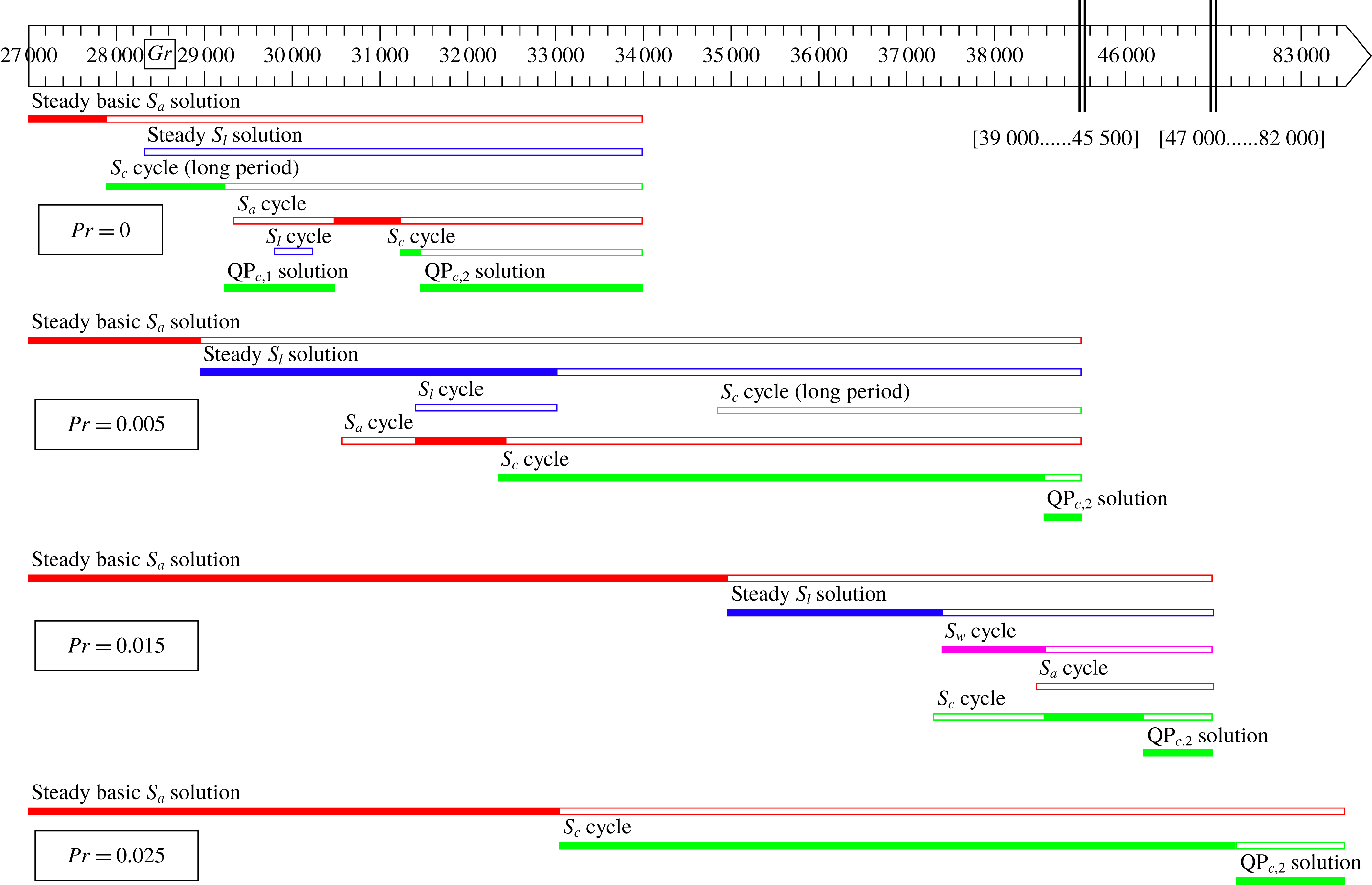
5.5 Global view of the solutions

A global presentation of the different solutions obtained when $Gr$ is increased for the four chosen Prandtl numbers is given in figure 11. The solutions are given by horizontal lines covering their domain of existence in terms of $Gr$ , these lines being solid lines in the range where the solutions are stable. As in the previous figures, different colours are used for the solutions, depending on their symmetries (green for the $S_{c}$ symmetry, red for the $S_{a}$ symmetry, blue for the $S_{l}$ symmetry and pink for the $S_{w}$ symmetry). For each Prandtl number, the solutions are presented from $Gr=27\,000$ up to values of $Gr$ allowing us to reach quasi-periodic states, i.e. $Gr=34\,000$ , 39 000, 47 000 and 83 500 for $Pr=0$ , 0.005, 0.015 and 0.025, respectively. We can see that many different solutions (steady, periodic, quasi-periodic) with different symmetries can be obtained. The path followed to go from the basic steady solution to the final quasi-periodic state through periodic states is different for each $Pr$ number studied. In any case, however, it was found that the last periodic solution is a $S_{c}$ cycle, which is then destabilized at a Naimark–Sacker bifurcation setting up a quasi-periodic state with the same $S_{c}$ symmetry.

Figure 11.

Global view of the existence range in terms of $Gr$ for all the solutions obtained from the basic steady solution to the quasi-periodic states for four Prandtl numbers in the range $0\leqslant Pr\leqslant 0.025$ . Coloured lines are used in order to easily identify the symmetry of the solutions, and these lines appear as solid lines in the $Gr$ range where the solutions are stable. Note that for a better global presentation of these results, the $Gr$ range is interrupted between 39 000 and 45 500 and between 47 000 and 82 000.

6 Change of the transition scenarios with $Pr$

Until now, we have presented some bifurcation analyses for different Prandtl numbers, but without connecting these cases between them. The idea is now to use these few examples to deepen our understanding of how the transition scenarios between the different observed stable solutions evolve when changing the Prandtl number.

The results presented in § 5 have shown that many Hopf bifurcation points, on the primary as well as on the secondary steady branch, are involved in the transition scenarios. There are also important connections between Hopf bifurcation points on the secondary branch and Hopf bifurcation points on the primary branch through interaction of cycles at pitchfork bifurcations: for example, $H_{l}^{S}$ is connected with $H_{a}^{P}$ through the interaction of the $S_{l}$ and $S_{a}$ cycles at $P_{l}^{C_{a}}$ and $H_{w,25}^{S}$ is connected with $H_{c,25}^{P}$ through the interaction of the $S_{w}$ and $S_{c}$ cycles at $P_{w}^{C_{c,25}}$ . Finally the transition scenarios appear to be strongly affected by the relative positions of the bifurcation points on the primary branch, i.e. $P_{l}^{P}$ , $H_{a}^{P}$ , $H_{c,0}^{P}$ and $H_{c,25}^{P}$ , and of the bifurcation points on the secondary branch, i.e. $H_{l}^{S}$ , $H_{w,0}^{S}$ and $H_{w,25}^{S}$ . The intersection of the paths of these different bifurcation points then plays an important role. All these intersections, already mentioned in § 4, are summarized in table 3, together with the $Pr$ ranges which are thus defined.

Table 3.

Intersection points of the paths of the main bifurcation points on the primary and secondary branches; $Pr$ ranges which are thus defined in the studied interval $0\leqslant Pr\leqslant 0.025$ .

For $1.63\times 10^{-2}\leqslant Pr\leqslant 2.5\times 10^{-2}$ , in the R6 range, the first bifurcation point is $H_{c,25}^{P}$ . We can then expect that in this range of $Pr$ , as for $Pr=0.025$ , $H_{c,25}^{P}$ will give an $S_{c}$ cycle which will evolve with the Grashof number and undergo a Naimark–Sacker bifurcation, allowing quasi-periodicity to set up.

For $1.44\times 10^{-2}\leqslant Pr\leqslant 1.63\times 10^{-2}$ , in the R5 range, the first bifurcation on the primary branch is now steady at $P_{l}^{P}$ due to the intersection of the $H_{c,25}^{P}$ and $P_{l}^{P}$ paths. This codimension-2 point leads also to the creation of the Hopf bifurcation $H_{w,25}^{S}$ on the secondary branch initiated at $P_{l}^{P}$ and of the pitchfork bifurcation of cycles $P_{w}^{C_{c,25}}$ on the $S_{c}$ cycle initiated at $H_{c,25}^{P}$ . In this range of $Pr$ , as for $Pr=0.015$ , we can expect to have a stable secondary branch up to the point $H_{w,25}^{S}$ , where a stable $S_{w}$ cycle is initiated. This $S_{w}$ cycle ends at $P_{w}^{C_{c,25}}$ , where it stabilizes the $S_{c}$ cycle, now unstable at its onset. A quasi-periodic state with $S_{c}$ symmetry will eventually appear when the $S_{c}$ cycle will be destabilized. Note that, in this range of $Pr$ , the $S_{a}$ cycle is expected to remain unstable and to play no role in the transition scenario.

The next changes, when decreasing $Pr$ , occur at $Pr_{c}=1.44\times 10^{-2}$ and $1.21\times 10^{-2}$ and correspond to the crossings of the $H_{c,25}^{P}$ and $H_{a}^{P}$ bifurcation points on the primary branch and the $H_{l}^{S}$ and $H_{w,25}^{S}$ bifurcation points on the secondary branch, respectively. Beyond these two crossings, in the R3 range, the dynamics found in the R5 range and involving the $S_{w}$ cycle and the $S_{c}$ cycle is now entirely unstable as these two cycles are affected by a supplementary unstable complex conjugate mode. As shown in figure 8(a) for $Pr=0.005$ , the important dynamics in this R3 range is connected with the $S_{l}$ and $S_{a}$ cycles: the secondary steady branch is stable up to $H_{l}^{S}$ , giving birth subcritically to an unstable $S_{l}$ cycle, which will eventually stabilize the $S_{a}$ cycle at the pitchfork point $P_{l}^{C_{a}}$ . Another pitchfork point on the $S_{a}$ cycle will give rise to a stable $S_{c}$ cycle and finally to a $\text{QP}_{c,2}$ state with central symmetry.

In the intermediate R4 range, the dynamics must be more complex as, compared to the R5 range, only the crossing of $H_{c,25}^{P}$ and $H_{a}^{P}$ on the primary branch has occurred. To have more information on the dynamics in this R4 range, we have calculated the bifurcation diagram for $Pr=0.013$ , which is presented in figure 12. We see that this diagram involves both the characteristics found in the R5 and R3 ranges. The $S_{w}$ cycle, stable at onset as in the R5 range, is now destabilized at a Naimark–Sacker bifurcation $H_{w}^{C_{w,25}}$ , before to disappear at the pitchfork bifurcation $P_{w}^{C_{c,25}}$ on the $S_{c}$ cycle coming from $H_{c,25}^{P}$ ( $Gr_{c}=38\,636$ ). This $S_{c}$ cycle, now two time unstable at onset, is then not stabilized. In contrast, as in the R3 domain, the $S_{a}$ cycle is only one-time unstable at onset at $H_{a}^{P}$ ( $Gr_{c}=35\,835$ ) and is stabilized at the pitchfork bifurcation $P_{l}^{C_{a}}$ to the $S_{l}$ cycle. Note that this $S_{l}$ cycle is two-time unstable at its subcritical onset at $H_{l}^{S}$ and a Naimark–Sacker bifurcation $H_{w}^{C_{l}}$ makes this cycle one-time unstable for smaller $Gr$ in order to fit with its stability at $P_{l}^{C_{a}}$ . As already seen, the $S_{a}$ cycle is then destabilized at a pitchfork point ( $Gr_{c}=38\,844$ ), which gives birth to a secondary $S_{c}$ cycle, slightly sub-critical at its origin, stable on a large domain of $Gr$ from $Gr_{c}=38\,767$ to $Gr_{c}=43\,665$ . The subsequent scenario is different from what was obtained for other values of $Pr$ . The $S_{c}$ cycle is destabilized by a period-doubling bifurcation initiating an $S_{c}$ cycle with a double period. This new $S_{c}$ cycle is destabilized at $Gr_{c}=46\,148$ at a pitchfork bifurcation giving rise to a $S_{w}$ cycle without symmetry stable up to $Gr_{c}=46\,646$ and then to a quasi-periodic state without symmetry, $\text{QP}_{w}$ . In fact, on the new $S_{c}$ cycle, there is also a Naimark–Sacker bifurcation very close to 46 148. The $\text{QP}_{c,3}$ quasi-periodic state with central symmetry which then appears is unstable at onset, but must be further stabilized as it can be obtained by time-stepping calculations at larger $Gr$ values as $Gr=46\,300$ and 46 600. There is then the coexistence of both quasi-periodic states without symmetry and with the $S_{c}$ symmetry in a certain range of $Gr$ values, as it was confirmed by time-stepping calculations at $Gr=46\,650$ .

Figure 12.

Bifurcation diagram ( $u^{\ast }$ versus $Gr$ ) for $Pr=0.013$ showing all the convective solutions from the stable steady solution with all the symmetries to the appearance of quasi-periodicity. As in the previous bifurcation diagrams, the $S_{a}$ cycle is red, the $S_{l}$ cycle is blue, the $S_{c}$ cycles are green and the $S_{w}$ cycles are pink. The stability of the different states is indicated by the number of unstable eigenvalues $n-m$ (see text in § 4). This case is intermediate between the cases at $Pr=0.015$ and $Pr=0.005$ and parts of their dynamics are found here. Note the occurrence of a period-doubling bifurcation at $Gr_{c}=43\,665$ , a specificity of this case.

A specificity of the R4 range is the existence of the Naimark–Sacker bifurcations $H_{w}^{C_{l}}$ and $H_{w}^{C_{w,25}}$ on the $S_{l}$ and $S_{w}$ cycles, respectively. Some extra calculations have shown that, for $Pr=0.0142$ , these bifurcation points $H_{w}^{C_{l}}$ and $H_{w}^{C_{w,25}}$ are close to the existence limit $P_{l}^{C_{a}}$ and $P_{w}^{C_{c,25}}$ of their respective cycles, whereas, for $Pr=0.0122$ , $H_{w}^{C_{l}}$ and $H_{w}^{C_{w,25}}$ are close to the birth points $H_{l}^{S}$ and $H_{w,25}^{S}$ of their respective cycles and also close to each other. All this means that the $H_{w}^{C_{l}}$ and $H_{w}^{C_{w,25}}$ points appear at $P_{l}^{C_{a}}$ and $P_{w}^{C_{c,25}}$ , respectively, when the $H_{a}^{P}$ and $H_{c,25}^{P}$ bifurcation points cross on the primary branch at $Pr_{c}=1.44\times 10^{-2}$ and that they disappear at $H_{l}^{S}$ and $H_{w,25}^{S}$ , when these $H_{l}^{S}$ and $H_{w,25}^{S}$ points cross on the secondary branch at $Pr_{c}=1.21\times 10^{-2}$ . This is also an indication that the stable part of the $S_{w}$ cycle, between $H_{w,25}^{S}$ and $H_{w}^{C_{w,25}}$ , very progressively shortens between $Pr=1.44\times 10^{-2}$ and $Pr=1.21\times 10^{-2}$ and eventually disappears at $Pr=1.21\times 10^{-2}$ .

The last crossings of bifurcation points occur on the primary branch, crossing of $H_{c,0}^{P}$ and $H_{a}^{P}$ at $Pr_{c}=3.28\times 10^{-4}$ and crossing of $H_{c,0}^{P}$ and $P_{l}^{P}$ at $Pr_{c}=8.83\times 10^{-5}$ , and they delimit the two ranges R2 and R1 of $Pr$ . Except for the limit case $Pr=0$ , we do not have bifurcation diagrams in these ranges and some extra calculations will then be necessary to understand the transition between the diagrams at $Pr=0.005$ and $Pr=0$ . We will follow interesting new bifurcation points appearing on the cycles in these $Pr$ ranges (figure 13) and compute a newly observed cycle for $Pr=0.0001$ (figure 14). Compared to the diagram at $Pr=0.005$ , the crossing of $H_{c,0}^{P}$ and $H_{a}^{P}$ at $Pr_{c}=3.28\times 10^{-4}$ will change the stability of the $S_{a}$ cycle at its onset at $H_{a}^{P}$ , with one pair of unstable complex conjugate Floquet multipliers in addition to the already unstable real Floquet multiplier. At the same time, however, a new Naimark–Sacker bifurcation $H_{c}^{C_{a}}$ appears on the $S_{a}$ cycle and stabilizes the pair of complex conjugate Floquet multipliers. As shown in figure 13, $H_{c}^{C_{a}}$ evolves from $H_{a}^{P}$ at $Pr=3.28\times 10^{-4}$ , crosses the path of $P_{l}^{C_{a}}$ , the other bifurcation on the $S_{a}$ cycle, at $Pr\approx 2.3\times 10^{-4}$ , before continuing towards $Pr=0$ . The appearance of this $H_{c}^{C_{a}}$ point allows the dynamics obtained at $Pr=0.005$ to remain, i.e. the stabilization of the $S_{a}$ cycle at $P_{l}^{C_{a}}$ and the further dynamics for larger $Gr$ , at least down to $Pr=2.3\times 10^{-4}$ . Indeed, for $Pr$ values below $2.3\times 10^{-4}$ , it is now above $H_{c}^{C_{a}}$ that the $S_{a}$ cycle is stabilized, in coherence with what is observed for $Pr=0$ . Note that the domain where the $S_{a}$ cycle is stable is highlighted in figure 13. Finally, the crossing of $H_{c}^{C_{a}}$ and $P_{l}^{C_{a}}$ also modifies the unstable spectrum of the $S_{l}$ cycle at $P_{l}^{C_{a}}$ , where it emerges from the $S_{a}$ cycle, as a pair of complex conjugate Floquet multipliers is now destabilized. We found, however, that the crossing also induces the creation of a new Naimark–Sacker bifurcation $H_{w}^{C_{l}}$ on the $S_{l}$ cycle, stabilizing these Floquet multipliers. Beyond $H_{w}^{C_{l}}$ , the unstable spectrum of the $S_{l}$ cycle is then the same as before the crossing, allowing the dynamics on the secondary branch to which the $S_{l}$ cycle is connected at $H_{l}^{S}$ to be maintained. $H_{w}^{C_{l}}$ will move all along the $S_{l}$ cycle, from $P_{l}^{C_{a}}$ at $Pr=2.3\times 10^{-4}$ to $H_{l}^{S}$ at $Pr=8.83\times 10^{-5}$ , i.e. at the crossing of $H_{c,0}^{P}$ and $P_{l}^{P}$ . This last crossing does not change the dynamics initiated from the primary branch and previously described.

Figure 13.

Paths of the bifurcation points in the very small $Pr$ range. In addition to the bifurcation points on the primary and secondary steady branches ( $P_{l}^{P}$ , $H_{c,0}^{P}$ , $H_{a}^{P}$ , $H_{l}^{S}$ and $H_{w,0}^{S}$ , as in figure 4 b), are given the bifurcation points on the $S_{a}$ cycle, steady bifurcation $P_{l}^{C_{a}}$ (sky-blue line, extrapolated with a dashed part) and Naimark–Sacker bifurcation $H_{c}^{C_{a}}$ (dark-blue line), and the bifurcation $H_{w}^{C_{l}}$ on the $S_{l}$ cycle calculated for $Pr=1\times 10^{-4}$ and $Pr=2.2\times 10^{-4}$ (black crosses) and interpolated in between (dashed black line). The domains where are stable the secondary steady flow (domain with oblique lines) and the $S_{a}$ cycle (domain with grey background) are highlighted. The bifurcation $H_{c}^{C_{c,0}}$ on the $S_{c,0}$ cycle is given for $Pr=0$ and $Pr=1\times 10^{-4}$ (red crosses) and interpolated in between (dashed red line). For $Pr\leqslant 8.83\times 10^{-5}$ , the $\text{QP}_{c,1}$ state can be obtained between $H_{c}^{C_{c,0}}$ and $H_{c}^{C_{a}}$ . Above $Pr=8.83\times 10^{-5}$ (dashed vertical black line), the $\text{QP}_{c,1}$ state is still observed in the $Gr$ range below $H_{c}^{C_{a}}$ and above the red asterisks, which define an approximate lower limit.

Figure 14.

Bifurcation diagram ( $u^{\ast }$ versus $Gr$ ) for $Pr=1\times 10^{-4}$ highlighting the $S_{c}$ cycle with long period (green colour) initiated at $H_{c,0}^{P}$ ( $Gr_{c}=28\,383$ , $f_{c}=2.79$ ) on the primary branch and unstable at this value of $Pr$ and the $S_{w}$ cycles with long periods (pink colours) initiated at the two points on the secondary branch belonging to the $H_{w,0}^{S}$ path. The $S_{w}$ cycle initiated at $Gr_{c}=28\,581$ (light-pink colour, $f_{c}=2.76$ ) is stable at onset and then destabilized at $Gr_{c}=29\,705$ at a Naimark–Sacker bifurcation, whereas the $S_{w}$ cycle initiated at $Gr_{c}=30\,004$ ( $f_{c}=2.20$ ) remains unstable. The steady secondary branch is stable from $P_{l}^{P}$ ( $Gr_{c}=28\,328$ ) to the first $H_{w,0}^{S}$ point, and then from the second $H_{w,0}^{S}$ point to $H_{l}^{S}$ ( $Gr_{c}=30\,386$ ).

We have now to describe the specific dynamics due to the bifurcation point $H_{w,0}^{S}$ that appears on the secondary branch at the crossing of $H_{c,0}^{P}$ and $P_{l}^{P}$ at $Pr_{c}=8.83\times 10^{-5}$ . $H_{w,0}^{S}$ will destabilize the secondary steady solution in a certain range of $Gr$ just above $Pr=8.83\times 10^{-5}$ (figure 13). This range of $Gr$ will shorten as $Pr$ is increased and disappear at $Pr\approx 1.1\times 10^{-4}$ . $H_{w,0}^{S}$ will also generate a stable $S_{w}$ cycle without symmetry and with a long period. This cycle is shown in figure 14 for $Pr=1\times 10^{-4}$ . It is stable from $Gr_{c}=28\,581$ , where it is initiated at $H_{w,0}^{S}$ ( $f_{c}=2.76$ ), to $Gr_{c}=29\,705$ , where is it destabilized at a Naimark–Sacker bifurcation and gives rise to a quasi-periodic state. This quasi-periodic state without symmetry was never observed as a stable state, meaning that the Naimark–Sacker bifurcation must be subcritical. In contrast, the $\text{QP}_{c,1}$ state with $S_{c}$ symmetry, which exists and is stable between $H_{c}^{C_{c,0}}$ and $H_{c}^{C_{a}}$ for $Pr=0$ and up to $Pr_{c}=8.83\times 10^{-5}$ in the R1 range, continues to be stable in a certain $Gr$ range above $Pr=8.83\times 10^{-5}$ despite the destabilization of the $S_{c}$ cycle. This $\text{QP}_{c,1}$ state was observed by time-stepping calculations below $H_{c}^{C_{a}}$ in a $Gr$ range decreasing in size with the increase of $Pr$ and disappearing at the crossing of $H_{c}^{C_{a}}$ and $P_{l}^{C_{a}}$ at $Pr=2.3\times 10^{-4}$ . This $Gr$ range can be seen in figure 14 between the $H_{c}^{C_{a}}$ curve and the red asterisks, which give the smallest $Gr$ values where the $\text{QP}_{c,1}$ state was obtained. Note finally that the second point $H_{w,0}^{S}$ appearing at $Gr_{c}=30\,004$ on the secondary branch, and restabilizing it, does not give rise to stable states as it can be observed in figure 14 for $Pr=1\times 10^{-4}$ . From all these results obtained for the very low values of $Pr$ , we can also conclude that the dynamics in the whole R1 range is similar to that obtained for $Pr=0$ , with only some variations of the main bifurcation points, $H_{c,0}^{P}$ , the onset of the stable $S_{c}$ cycle with long period, $H_{c}^{C_{c,0}}$ , the onset of the stable $\text{QP}_{c,1}$ state and $H_{c}^{C_{a}}$ , the limit of the $\text{QP}_{c,1}$ state and onset of the stable $S_{a}$ cycle (see figure 13).

We finally give a summary of all the different stable flow states, from steady to quasi-periodic, which have been obtained in the study for $0\leqslant Pr\leqslant 0.025$ in table 4. We also indicate in which domain of $Pr$ from R1 to R6 (see table 3) they can be found. Fourteen different stable states have been obtained, corresponding to two steady states, eight cycles and four quasi-periodic states. We see that, besides the basic $S_{a}$ steady state, the quasi-periodic $\text{QP}_{c,2}$ state is found in all the $Pr$ ranges. The primary $S_{c}$ cycle is stable for the largest values of $Pr$ in ranges R5 and R6, whereas the primary $S_{a}$ cycle, although never stable at its onset, is obtained as a stable state in the other ranges R4 to R1 and gives birth to a stable secondary $S_{c}$ cycle. The secondary $S_{w}$ cycle is stable in R5 where it also stabilizes the primary $S_{c}$ cycle, but also in R4 in a shrinking interval of $Gr$ . In contrast, the secondary $S_{l}$ cycle is never obtained as a stable state, although it is involved in the stabilization of the $S_{a}$ cycle. The long-period primary $S_{c}$ cycle is only stable in R1, but another long-period secondary $S_{w}$ cycle is stable in a very small range of $Pr$ inside R2. The quasi periodic $\text{QP}_{c,1}$ state, stable in R1 and part of R2, has the peculiarity of being an intermediate state between stable cycles. Finally, the largest number of stable states is obtained in R4, which appears as a range of $Pr$ where transition between different bifurcation scenarios occurs.

Table 4.

Summary of the different stable flow states, from steady to quasi-periodic, which have been obtained in the study and the domains of $Pr$ from R1 to R6 (see table 3) where they can be found. The cycles are given as primary when they are initiated at a Hopf bifurcation on the steady primary branch and as secondary when they are initiated at a Hopf bifurcation on the steady secondary branch or at a pitchfork bifurcation on another cycle.