1 Introduction
Turbulent flows contain a very large number of scales of motion, which increases with the Taylor microscale Reynolds number (
 $Re_{\unicode[STIX]{x1D706}}$
). This is compounded by the complex way the energy is shifted between these scales and poses a strong challenge to any theoretical analysis of turbulence. It was recognised at an early stage that one is forced to introduce some sort of phenomenology in the form of hypotheses regarding the geometry and dynamics of turbulent flows in order to develop a theory of turbulence. The first phenomenological argument, which is an idealisation of turbulence, assumes that turbulence is homogeneous and isotropic. Such an idealisation simplifies the problem considerably and leads to the most important equation for homogeneous isotropic turbulence (HIT), namely the Kármán–Howarth (KH) equation (Kármán & Howarth Reference Kármán and Howarth1938). Starting with the Navier–Stokes equations (hereafter denoted NSEq), those authors developed a dynamical equation for the longitudinal velocity correlation coefficient
 $f(r,t)\equiv \overline{u(x,t)u(x+r,t)}/u^{^{\prime }2}(t)$
for isotropic turbulence (
 $u$
is the velocity fluctuation,
 $r$
is a spatial increment, the prime denotes a root mean square value and the overbar represents spatial averaging). The KH equation is
 $$\begin{eqnarray}\frac{\unicode[STIX]{x2202}(u^{^{\prime }2}f)}{\unicode[STIX]{x2202}t}=2\left[\frac{\unicode[STIX]{x2202}(u^{^{\prime }3}h)}{\unicode[STIX]{x2202}r}+\frac{4(u^{^{\prime }3}h)}{r}\right]+2\unicode[STIX]{x1D708}\left[\frac{\unicode[STIX]{x2202}^{2}(u^{^{\prime }2}f)}{\unicode[STIX]{x2202}r^{2}}+\frac{4}{r}\frac{\unicode[STIX]{x2202}(u^{^{\prime }2}f)}{\unicode[STIX]{x2202}r}\right]\!,\end{eqnarray}$$
where
 $h$
is the triple velocity correlation (
 $\equiv \overline{u^{2}(x,t)u(x+r,t)}/u^{^{\prime }3}$
) (for convenience we dropped the variables
 $r$
and
 $t$
with the explicit understanding that
 $f$
and
 $h$
are functions of both variables; we also dropped
 $x$
and
 $t$
from other quantities such as
 $u$
). The term on the left-hand side of the equation represents the temporal variation. On the right-hand side, the first and second terms represent the nonlinear interactions between velocity components, and the bracketed term corresponds to the viscous effect or viscous diffusion. This equation, which marked a milestone in the study of isotropic turbulence, is of great interest because it imposes constraints on the values of
 $f$
and
 $h$
. However, to carry out further analysis Kármán & Howarth (Reference Kármán and Howarth1938) introduced a second phenomenological argument which allows the KH equation to be reduced to an ordinary differential equation. This second argument, often called self-preservation, states that the shapes of
 $f$
and
 $h$
remain unchanged for different values of time when properly normalised. For small Reynolds numbers, which allows the term involving
 $h$
to be neglected, Kármán & Howarth (Reference Kármán and Howarth1938) assumed that
 $f$
is a function of
 $\unicode[STIX]{x1D712}=r/\sqrt{\unicode[STIX]{x1D708}t}$
. For very large Reynolds numbers, they discussed the case of grid turbulence and assumed that both
 $f$
and
 $h$
are functions of
 $\unicode[STIX]{x1D713}=r/L$
, where
 $L$
is a function of
 $M$
, the grid mesh size, and
 $Ut$
(
 $U$
is the mean flow velocity).
Scale-invariance similarity, to which self-preservation belongs and dimensional analysis is intimately linked (Barenblatt Reference Barenblatt1996; Tsinober Reference Tsinober2009), states that under the scale transformation
 $x^{\ast }=\unicode[STIX]{x1D6FC}x,t^{\ast }=\unicode[STIX]{x1D6FD}t$
, where
 $\unicode[STIX]{x1D6FC}$
and
 $\unicode[STIX]{x1D6FD}$
are arbitrary positive quantities, the equations of motion remain unchanged or invariant. Of particular interest is the role that scale invariance plays in the 1941 Kolmogorov theory of turbulence, as commonly denoted by K41 (Frisch Reference Frisch1995; Tsinober Reference Tsinober2009); Yaglom (Reference Yaglom1994) recalls that prior to publishing his K41 theory (Kolmogorov Reference Kolmogorov1941a
), Kolmogorov ‘stated that self-similarity must imply proportionality of the longitudinal structure function
 $\overline{(\unicode[STIX]{x1D6FF}u)^{2}}$
to some power of
 $r^{m}$
for a wide range of
 $r$
values’. Although Kolmogorov did not specifically mention scale invariance in his 1941 paper, he certainly used it (see § 5) when he proposed his two similarity hypotheses for isotropic small-scale turbulence which led him to provide a solution for
 $\overline{(\unicode[STIX]{x1D6FF}u)^{2}}$
, with no reference to the NSEq. The first hypothesis allowed him to obtain the scaling length (
 $\unicode[STIX]{x1D702}=(\unicode[STIX]{x1D708}^{3}/\overline{\unicode[STIX]{x1D716}})^{1/4}$
) and velocity scale (
 $v_{K}=(\unicode[STIX]{x1D708}\overline{\unicode[STIX]{x1D716}})^{1/4}$
). He further obtained, using dimensional arguments, the two-thirds similarity law, namely
 $\overline{(\unicode[STIX]{x1D6FF}u)^{2}}\sim (\overline{\unicode[STIX]{x1D716}}r)^{2/3}$
when
 $\unicode[STIX]{x1D702}\ll r\ll L$
(
 $L$
is an integral length scale) for very large
 $Re_{\unicode[STIX]{x1D706}}$
. However, at the 1961 international colloquium in Marseille, Kolmogorov revealed an apparent flaw in his theory, namely the neglect of the large-scale fluctuations of
 $\unicode[STIX]{x1D716}$
, an issue first raised by Landau (see for example Landau & Lifshitz (Reference Landau and Lifshitz1987)) shortly after K41 was published. Kolmogorov (Reference Kolmogorov1962) proposed his refined similarity hypotheses (referred to as K62) to account for such fluctuations. There is, however, one exact result. This is the four-fifths law or
 $\overline{(\unicode[STIX]{x1D6FF}u)^{3}}=(4/5)\overline{\unicode[STIX]{x1D716}}r$
derived rigorously by Kolmogorov from the transport equation for
 $\overline{(\unicode[STIX]{x1D6FF}u)^{2}}$
(Kolmogorov Reference Kolmogorov1941b
) and which does not require any phenomenological argument such as scale invariance. Since it is derived from the NSEq, this law must be satisfied by any theory of small-scale turbulence when the Reynolds number is infinite.
The present paper, which follows and expands on our recent studies (Antonia, Djenidi & Danaila Reference Antonia, Djenidi and Danaila2014; Antonia et al.
Reference Antonia, Tang, Djenidi and Danaila2015, Reference Antonia, Djenidi, Danaila and Tang2017; Djenidi & Antonia Reference Djenidi and Antonia2015; Djenidi, Antonia & Danaila Reference Djenidi, Antonia and Danaila2017a
; Djenidi et al.
Reference Djenidi, Danaila, Antonia and Tang2017b
), closely examines the consequences of scale-invariance similarity in the context of HIT. The consequences of scale-invariance similarity for small-scale turbulence have been mainly investigated using phenomenological arguments; this is how, for example, Kolmogorov obtained his similarity hypotheses and similarity laws (Kolmogorov Reference Kolmogorov1941a
) for infinitely large Reynolds numbers. Since scale invariance is an exact property of the NSEq (Frisch Reference Frisch1995; Henriksen Reference Henriksen2015), we investigate in this work its consequences within the framework of the NSEq at finite Reynolds numbers in order to obtain rigorous theoretical results independently of the theory of Kolmogorov and against which phenomenological results can be tested and compared. It is important to distinguish between the scaling properties of the NSEq, which map any solutions of these equations to other solutions, and the assumption of self-preservation which assumes particular form of the NSEq. So far, only self-preservation solutions as introduced by Kármán & Howarth (Reference Kármán and Howarth1938) have been considered. For example, Djenidi et al. (Reference Djenidi, Antonia and Danaila2017a
,Reference Djenidi, Danaila, Antonia and Tang
b
) considered self-preservation solutions of the structure functions and showed that the Kolmogorov scaling emerges naturally from the NSEq and developed an expression for the flatness factor of the longitudinal velocity derivative. Thiesset, Antonia & Djenidi (Reference Thiesset, Antonia and Djenidi2014) investigated the consequences of self-preservation for the dissipative range along the axis of a turbulent round jet. Here, the analysis, which considers both the dissipative and scaling ranges, exploits the scale-invariance property of the NSEq. This expands the generality of our previous results and, as we will see later, allows us to derive the
 $n$
-thirds law (i.e.
 $\overline{(\unicode[STIX]{x1D6FF}u)^{n}}\sim r^{n/3}$
) without resorting to asymptotic matching expansions (Gamard & George Reference Gamard and George2000; Lundgren Reference Lundgren2002). The analysis, which is tested against experimental data, is carried out on the transport equations for
 $\overline{(\unicode[STIX]{x1D6FF}u)^{2}}$
and
 $\overline{(\unicode[STIX]{x1D6FF}u)^{3}}$
. The equation for
 $\overline{(\unicode[STIX]{x1D6FF}u)^{2}}$
, first introduced by Kolmogorov (Reference Kolmogorov1941b
) and which plays a pivotal role in the theory of turbulence, has been exploited extensively, particularly when assessing K41. Kolmogorov (Reference Kolmogorov1941b
) used the hypothesis of scale invariance for this equation to derive the two-thirds similarity law for an infinitely large Reynolds number. The equation for
 $\overline{(\unicode[STIX]{x1D6FF}u)^{3}}$
has received much less attention (e.g. Hill & Boratav Reference Hill and Boratav2001; Yakhot Reference Yakhot2001; Gotoh & Nakano Reference Gotoh and Nakano2003; Djenidi et al.
Reference Djenidi, Danaila, Antonia and Tang2017b
). Our motivation for focusing on the transport equations for
 $\overline{(\unicode[STIX]{x1D6FF}u)^{2}}$
and
 $\overline{(\unicode[STIX]{x1D6FF}u)^{3}}$
is that it allows us to assess rigorously the constraints imposed by the scale-invariance property of the equations in finite Reynolds number HIT and should yield results free from phenomenology.
2 Equations of motion, scale-invariance symmetry and self-preservation
The transport equations for the second- and third-order moments of the longitudinal velocity increment to be considered have already been written by Djenidi et al. (Reference Djenidi, Antonia and Danaila2017a
,Reference Djenidi, Danaila, Antonia and Tang
b
). We reproduce their derivation in appendix A.1 for convenience. In the next section we use the scale-invariance property of the NSEq to discuss its consequences for the equations of motion (A 7) and (A 8) and the behaviour of
 $\unicode[STIX]{x1D6FF}u_{n}(\equiv \overline{(\unicode[STIX]{x1D6FF}u)^{n}})$
for
 $n=2$
, 3 and 4.
2.1 Scale-invariance symmetry
It is well known that the NSEq satisfies a series of symmetries. For example, Frisch (Reference Frisch1995) lists the following symmetries for the NSEq: time-invariance, space-invariance, rotation-invariance, reflection-invariance, Galilean-invariance, parity-invariance and scale-invariance symmetries. There is also pressure-invariance symmetry (Oberlack Reference Oberlack1997). In the present work we focus on scale-invariance symmetry only. Scale-invariance symmetry (Frisch Reference Frisch1995; Henriksen Reference Henriksen2015) is described by
 $$\begin{eqnarray}x\rightarrow \unicode[STIX]{x1D6FE}x,t\rightarrow \unicode[STIX]{x1D6FE}^{1-q}t,u\rightarrow \unicode[STIX]{x1D6FE}^{q}u,\end{eqnarray}$$
where
 $\unicode[STIX]{x1D6FE}$
is a scale positive factor and
 $q$
is a scaling exponent (positive or negative). When (2.1) is applied, all terms of the NSEq are multiplied by
 $\unicode[STIX]{x1D6FE}^{2q-1}$
apart from the viscous term which is multiplied by
 $\unicode[STIX]{x1D6FE}^{q-2}$
. If
 $\unicode[STIX]{x1D708}\neq 0$
then
 $q=-1$
, which restricts dramatically the invariance conditions for a finite
 $Re$
. For example, this restriction (i.e.
 $q=-1$
) imposes a constant Reynolds number. Indeed, for example,
 $Re=xu/\unicode[STIX]{x1D708}\rightarrow \unicode[STIX]{x1D6FE}x(\unicode[STIX]{x1D6FE}^{q}u)/\unicode[STIX]{x1D708}$
which, with
 $q=-1$
, remains unchanged. Thus, the NSEq is scale-invariant under the following rescaling:
 $$\begin{eqnarray}r^{\ast }=r/\unicode[STIX]{x1D6FC},\quad t^{\ast }=t/\unicode[STIX]{x1D6FD},\quad u^{\ast }=u/\unicode[STIX]{x1D707},\end{eqnarray}$$
where
 $\unicode[STIX]{x1D6FC}$
,
 $\unicode[STIX]{x1D6FD}$
and
 $\unicode[STIX]{x1D707}$
are positive and, in general, arbitrary, and with
 $u^{\ast }=r^{\ast -1}$
and
 $t^{\ast }=r^{\ast -2}$
so compliance with
 $q=-1$
is satisfied.
We expect that the scale-invariance property of the NSEq should also be a property of any transport equation derived from the NSEq. To establish that this is indeed the case for the present transport equations of
 $\overline{(\unicode[STIX]{x1D6FF}u)^{2}}$
and
 $\overline{(\unicode[STIX]{x1D6FF}u)^{3}}$
, we apply scaling (2.1) to (A 7), for example. Thus, we have
 $\unicode[STIX]{x1D6FF}u_{n}\rightarrow \unicode[STIX]{x1D6FE}^{nq}\unicode[STIX]{x1D6FF}u_{n}$
(
 $n=2$
and 3),
 $\overline{\unicode[STIX]{x1D716}}\rightarrow \unicode[STIX]{x1D6FE}^{3q-1}\overline{\unicode[STIX]{x1D716}}$
and
 $$\begin{eqnarray}\unicode[STIX]{x1D6FF}u_{3}\unicode[STIX]{x1D6FE}^{3q}=6\unicode[STIX]{x1D708}\unicode[STIX]{x1D6FE}^{2q-1}\frac{\unicode[STIX]{x2202}\unicode[STIX]{x1D6FF}u_{2}}{\unicode[STIX]{x2202}r}-\frac{3}{r^{4}}\unicode[STIX]{x1D6FE}^{3q}\int _{0}^{r}s^{4}\frac{\unicode[STIX]{x2202}\unicode[STIX]{x1D6FF}u_{2}}{\unicode[STIX]{x2202}t}\,\text{d}s-\frac{4}{5}\unicode[STIX]{x1D6FE}^{3q}\overline{\unicode[STIX]{x1D716}}r,\end{eqnarray}$$
which shows that
 $q=-1$
if scale invariance is to be observed with
 $\unicode[STIX]{x1D708}\neq 0$
. Otherwise, scale invariance is verified for any real value of
 $q$
when
 $\unicode[STIX]{x1D708}=0$
. As expected, similar results (not shown here) are obtained by applying the scaling (2.1) to (A 8). Introducing the scaled variables (2.2), which lead to
 $$\begin{eqnarray}\unicode[STIX]{x1D6FF}u^{\ast }=\unicode[STIX]{x1D6FF}u/\unicode[STIX]{x1D707},\quad \overline{\unicode[STIX]{x1D716}^{\ast }}=\overline{\unicode[STIX]{x1D716}}\unicode[STIX]{x1D6FC}/\unicode[STIX]{x1D707}^{3},\end{eqnarray}$$
into (A 7) yields
 $$\begin{eqnarray}\unicode[STIX]{x1D6FF}u_{3}^{\ast }=6\frac{\unicode[STIX]{x1D708}}{(\unicode[STIX]{x1D707}\unicode[STIX]{x1D6FC})}\frac{\unicode[STIX]{x2202}\unicode[STIX]{x1D6FF}u_{2}^{\ast }}{\unicode[STIX]{x2202}r^{\ast }}-\frac{3}{r^{\ast 4}}\left(\frac{\unicode[STIX]{x1D6FC}^{2}}{(\unicode[STIX]{x1D707}\unicode[STIX]{x1D6FC})\unicode[STIX]{x1D6FD}}\right)\int _{0}^{r^{\ast }}s^{\ast 4}\frac{\unicode[STIX]{x2202}\unicode[STIX]{x1D6FF}u_{2}^{\ast }}{\unicode[STIX]{x2202}t^{\ast }}\,\text{d}s^{\ast }-\frac{4}{5}\overline{\unicode[STIX]{x1D716}^{\ast }}r^{\ast }.\end{eqnarray}$$
For the scaling (2.2) to leave (2.5) scale-invariant, one must have
 $$\begin{eqnarray}\frac{\unicode[STIX]{x1D707}\unicode[STIX]{x1D6FC}}{\unicode[STIX]{x1D708}}=C_{1},\quad \frac{\unicode[STIX]{x1D6FC}}{\unicode[STIX]{x1D707}\unicode[STIX]{x1D6FD}}=C_{2},\end{eqnarray}$$
with
 $C_{1}=C_{2}=1$
. We note that
 $C_{1}$
is in fact a scaling Reynolds number that we hereafter denote
 $Re_{\unicode[STIX]{x1D6FC}}$
. Note that at this stage of the analysis, nothing is known of the actual length scale
 $\unicode[STIX]{x1D6FC}$
and velocity scale
 $\unicode[STIX]{x1D707}$
. The main important result so far is that the scale-invariance property of the equations imposes
 $\unicode[STIX]{x1D707}\unicode[STIX]{x1D6FC}/\unicode[STIX]{x1D708}=1$
. We can, however, determine the actual expressions for
 $\unicode[STIX]{x1D6FC}$
and
 $\unicode[STIX]{x1D707}$
as follows. We write
 $\unicode[STIX]{x1D707}=Re_{\unicode[STIX]{x1D6FC}}\unicode[STIX]{x1D708}/\unicode[STIX]{x1D6FC}$
which, when substituted into the expression for
 $\overline{\unicode[STIX]{x1D716}^{\ast }}$
, yields
 $$\begin{eqnarray}\unicode[STIX]{x1D6FC}=Re_{\unicode[STIX]{x1D6FC}}^{3/4}\overline{\unicode[STIX]{x1D716}^{\ast }}^{1/4}\left(\frac{\unicode[STIX]{x1D708}^{3}}{\overline{\unicode[STIX]{x1D716}}}\right)^{1/4}.\end{eqnarray}$$
Now substituting (2.7) again into the expression for
 $\overline{\unicode[STIX]{x1D716}^{\ast }}$
leads to
 $$\begin{eqnarray}\unicode[STIX]{x1D707}=\left(\frac{Re_{\unicode[STIX]{x1D6FC}}^{1/4}}{\overline{\unicode[STIX]{x1D716}^{\ast }}^{1/4}}\right)\left(\unicode[STIX]{x1D708}\overline{\unicode[STIX]{x1D716}}\right)^{1/4}.\end{eqnarray}$$
As seen above, the property of scale invariance imposes
 $Re_{\unicode[STIX]{x1D6FC}}=1$
. If
 $\overline{\unicode[STIX]{x1D716}^{\ast }}=1$
, then
 $\unicode[STIX]{x1D6FC}=(\unicode[STIX]{x1D708}^{3}/\overline{\unicode[STIX]{x1D716}})^{1/4}$
 $(\equiv \unicode[STIX]{x1D702})$
and
 $\unicode[STIX]{x1D707}=(\unicode[STIX]{x1D708}\overline{\unicode[STIX]{x1D716}})^{1/4}$
(
 $\equiv v_{K}$
), the Kolmogorov length and velocity scales, and (2.5) becomes
 $$\begin{eqnarray}\unicode[STIX]{x1D6FF}u_{3}^{\ast }=6\frac{\unicode[STIX]{x2202}\unicode[STIX]{x1D6FF}u_{2}^{\ast }}{\unicode[STIX]{x2202}r^{\ast }}-\frac{3}{r^{\ast 4}}\left(\frac{\unicode[STIX]{x1D702}^{2}}{\unicode[STIX]{x1D708}\unicode[STIX]{x1D6FD}}\right)\int _{0}^{r^{\ast }}s^{\ast 4}\frac{\unicode[STIX]{x2202}\unicode[STIX]{x1D6FF}u_{2}^{\ast }}{\unicode[STIX]{x2202}t^{\ast }}\,\text{d}s^{\ast }-\frac{4}{5}r^{\ast },\end{eqnarray}$$
which indicates that scale invariance imposes also the following relation between
 $\unicode[STIX]{x1D702}$
and
 $\unicode[STIX]{x1D6FD}$
:
 $$\begin{eqnarray}\unicode[STIX]{x1D702}=\sqrt{\unicode[STIX]{x1D708}\unicode[STIX]{x1D6FD}}.\end{eqnarray}$$
2.2 Self-preservation
We now examine the case when self-preservation (or self-similarity) solutions of the equations for
 $\overline{(\unicode[STIX]{x1D6FF}u)^{2}}$
and
 $\overline{(\unicode[STIX]{x1D6FF}u)^{2}}$
are assumed when the flow evolves in time or space. Recall that self-preservation solutions are in general not a consequence of the scale-invariance property of the equations of motion; however, they leave the equations unchanged during decay. Self-preservation solutions were extensively investigated by Townsend (Reference Townsend1956, Reference Townsend1976). Self-preservation is simply similarity of shape of statistical functions during decay in time or space, i.e. the shape of any statistical function, when adequately renormalised, remains unchanged during decay. We start the analysis with the final results of the work of Djenidi et al. (Reference Djenidi, Antonia and Danaila2017a
) who applied self-preservation to (A 7) and (A 8) (see appendix A.2 where we reproduce the details of the calculations). It is found that the length scale
 $l=(\sqrt{C_{5}}C_{1})^{1/2}(\unicode[STIX]{x1D708}^{3}/\overline{\unicode[STIX]{x1D716}})^{1/4}$
(A 23) and velocity scale
 $u_{2}=(C_{1}/\sqrt{C_{5}})^{1/2}(\unicode[STIX]{x1D708}\overline{\unicode[STIX]{x1D716}})^{1/4}$
(A 24) emerge naturally from the equations (see appendix A for details on the constants
 $C_{1}$
and
 $C_{5}$
). Thus, any scaling variables proportional to the Kolmogorov scales are proper scaling variables. Since we can write
 $C_{5}=(\overline{\unicode[STIX]{x1D716}}l/v_{k}^{3})Re_{l}$
, we then recover (2.7) and (2.8), illustrating the relation between self-preservation and scale invariance as represented by (2.1). The selection of the scaling variables
 $l$
and
 $u_{2}$
fixes the values of the constants
 $C_{1}$
and
 $C_{5}$
. For example, using
 $\unicode[STIX]{x1D702}$
and
 $v_{K}$
leads to
 $C_{1}=1$
and
 $C_{5}=1$
, and using
 $\unicode[STIX]{x1D706}$
and
 $u^{\prime }$
leads to
 $C_{1}=Re_{\unicode[STIX]{x1D706}}$
and
 $C_{5}=15$
. In the rest of the paper, we use the former selection of (
 $l,u_{2}$
) since they lead to
 $Re_{\unicode[STIX]{x1D6FC}}=\overline{\unicode[STIX]{x1D716}^{\ast }}=1$
. Of course, any choice of
 $l$
and
 $u_{2}$
satisfying the constraints (A 18) and (A 22) is valid and can be used without affecting the analysis and conclusions.
Kármán & Howarth (Reference Kármán and Howarth1938) introduced the time-varying length scale
 $\sqrt{\unicode[STIX]{x1D708}t}$
to investigate the decay of HIT and seek a self-preserving solution for
 $f(r^{\ast })$
(i.e. the shape of
 $f$
remains the same at all instants). This scaling is equivalent to setting
 $\unicode[STIX]{x1D6FD}=t$
in (2.10) which makes
 $t^{\ast }$
constant (i.e. removing explicitly the time dependence in the normalised structure functions). This in turn leads to
 $\unicode[STIX]{x1D6FC}=\sqrt{\unicode[STIX]{x1D708}t}$
; the second term on the right-hand side of (2.5) should then be expanded to reflect the time dependence of
 $\unicode[STIX]{x1D6FC}$
, as shown in (A 16), for example. Interestingly, the constraint (A 20) leads to
 $l\sim \sqrt{\unicode[STIX]{x1D708}t}$
, which under the first constraint of (A 18) yields
 $u_{2}\sim 1/(\sqrt{\unicode[STIX]{x1D708}t})$
, illustrating that the self-preservation solutions sought by Kármán & Howarth (Reference Kármán and Howarth1938) and Djenidi et al. (Reference Djenidi, Antonia and Danaila2017a
), for example, are compatible with the scale-invariance property of the equations. In that context, and in hindsight, it is then not surprising that Djenidi et al. (Reference Djenidi, Antonia and Danaila2017a
) arrived at the Kolmogorov scaling, since, as shown in (§ 2.1), that scaling is a consequence of the scale-invariance property of the NSEq.
2.3 Scale invariance at infinitely large Reynolds number
A comment on the very large Reynolds number case is warranted. As will be shown in § 3, the second term on the right-hand side of (A 7) becomes negligible and can be removed for very large Reynolds numbers. Thus, equation (A 7) reduces to the Kolmogorov equation used to derive the
 $4/5$
law (Kolmogorov Reference Kolmogorov1941b
). Both (2.5) and (A 16) without the integral terms are still valid and lead to the same scaling (i.e. Kolmorogov’s scaling). If we now consider only the range of separation,
 $r^{\ast }$
, for which the viscous term also becomes negligible, then we can write both equations as
 $$\begin{eqnarray}\unicode[STIX]{x1D6FF}u_{3}^{\ast }={\textstyle \frac{4}{5}}\overline{\unicode[STIX]{x1D716}^{\ast }}r^{\ast }.\end{eqnarray}$$
Note that the scaling exponent
 $q$
can no longer be equal to
 $-1$
. To show it, we follow the example of Davidson (Reference Davidson2015). Scale invariance implies
 $$\begin{eqnarray}\overline{(\unicode[STIX]{x1D6FF}u(\unicode[STIX]{x1D6FE}r))^{p}}=\unicode[STIX]{x1D6FE}^{pq}\overline{(\unicode[STIX]{x1D6FF}u(r))^{p}}.\end{eqnarray}$$
Thus, for
 $p=3$
we have
 $$\begin{eqnarray}\overline{(\unicode[STIX]{x1D6FF}u(\unicode[STIX]{x1D6FE}r))^{3}}=\unicode[STIX]{x1D6FE}^{3q}\overline{(\unicode[STIX]{x1D6FF}u(r))^{3}}=\unicode[STIX]{x1D6FE}^{3q}(-{\textstyle \frac{4}{5}}\overline{\unicode[STIX]{x1D716}}r)=\unicode[STIX]{x1D6FE}^{3q-1}(-{\textstyle \frac{4}{5}}\overline{\unicode[STIX]{x1D716}}\unicode[STIX]{x1D6FE}r).\end{eqnarray}$$
Since
 $\overline{(\unicode[STIX]{x1D6FF}u(\unicode[STIX]{x1D6FE}r))^{3}}=-4/5\overline{\unicode[STIX]{x1D716}}\unicode[STIX]{x1D6FE}r$
, it follows that
 $q=1/3$
in (2.13). This would appear to lead to a paradox because we saw that scale invariance also imposes
 $q=-1$
in order to achieve a constant scaling Reynolds number when
 $\unicode[STIX]{x1D708}\neq 0$
. However, this paradox can be lifted by noting that (2.11) corresponds to the case
 $\unicode[STIX]{x1D708}=0$
for which
 $q$
can be different from
 $-1$
. Further, combining the first expression of (A 18) with (A 22) (constraints (A 19)–(A 21) are no longer relevant in (2.11)) leads to
 $(\overline{\unicode[STIX]{x1D716}}l/u_{2}^{3})=C$
or
 $\overline{\unicode[STIX]{x1D716}}=Cu_{2}^{3}/l$
. Since
 $\overline{\unicode[STIX]{x1D716}}$
is independent of
 $r$
, we can write
 $\overline{\unicode[STIX]{x1D716}}=C\unicode[STIX]{x1D6FE}^{3q}u_{2}^{3}/(\unicode[STIX]{x1D6FE}l)=C\unicode[STIX]{x1D6FE}^{3q-1}u_{2}^{3}/l$
, so that
 $q=1/3$
once again; this is an alternative method to the Davidson one to derive
 $q=1/3$
.
Let us now consider the dissipative range only. Both (2.5) and (A 16) lead, after integration, to
 $$\begin{eqnarray}\overline{(\unicode[STIX]{x1D6FF}u)^{2}}=\frac{1}{15\unicode[STIX]{x1D708}}\overline{\unicode[STIX]{x1D716}}r^{2}.\end{eqnarray}$$
Scale invariance implies
 $\overline{(\unicode[STIX]{x1D6FF}u(\unicode[STIX]{x1D6FE}r))^{2}}=\unicode[STIX]{x1D6FE}^{2q}\overline{(\unicode[STIX]{x1D6FF}u(r))^{2}}$
. If we now apply the same procedure as in (2.13) we find
 $q=1$
, leading to a scaling exponent different from that for the inertial range. The scaling exponent
 $q$
in the dissipative range differs from that in the inertial range since the dynamics of the turbulence in the two regions is different; in particular, and according to (2.11) and (2.14), the inertial range is controlled only by
 $\overline{\unicode[STIX]{x1D716}}$
while the dissipative range is controlled by
 $\overline{\unicode[STIX]{x1D716}}$
and
 $\unicode[STIX]{x1D708}$
. It is worth noting that while
 $\unicode[STIX]{x1D708}$
cannot be considered zero in the dissipative range, the exponent
 $q$
differs from
 $-1$
, which again would appear paradoxical. This is nevertheless not the case, since (2.14) (and (2.11) for that matter) is a different equation from (A 7) and thus cannot have the same solution as (A 7).
The previous observations warrant further discussion. Scale invariance, when imposed at all scales of motion, requires that the entire shape (or profile) of a solution remains unchanged after being appropriately rescaled. For example, during turbulence decay, the shape of the distribution
 $\overline{(\unicode[STIX]{x1D6FF}u^{\ast })^{3}}(r^{\ast })$
should remain unchanged when scaled using the Kolmogorov scales (for a given
 $Re_{\unicode[STIX]{x1D706}}$
). This has been verified experimentally and numerically and indicates that two grid turbulence experiments with geometrically similar grids but with different mesh sizes will lead to the same distribution of
 $\overline{(\unicode[STIX]{x1D6FF}u^{\ast })^{3}}(r^{\ast })$
if the Reynolds number based on the grid mesh size,
 $Re_{M}$
, is the same between the two experiments. This differs from the case where scale invariance is sought over a limited range of scales such as in the inertial range. This necessitates considering a rather incomplete equation. For example, to obtain (2.11) both the viscous and the large-scale terms are neglected, which invariably changes the dynamics of the flow and leads to different solutions since both initial and boundary conditions also change. This is why it is quite difficult to test both experimentally and numerically theoretical solutions based on approximate equations; the various assumptions made to reduce the complexity of the equations are not necessarily met in the experiments and/or the numerical simulations.
Since we established the equivalence between (2.7), (2.8) and (A 23), (A 24), and, more importantly, at least for HIT, that self-preservation solutions are compatible with the scale-invariance symmetry of the equations of motion, we hereafter will not distinguish between self-similarity, self-preservation and scale invariance, and we simply use the terminology scale invariance in the rest of the paper. We note that scale invariance does not require infinite scaling Reynolds number. For decaying HIT, for example, scale invariance can exist (the shape of the normalised distribution
 $\overline{(\unicode[STIX]{x1D6FF}u)^{2}}$
remains fixed during the decay) for any given Reynolds numbers. However, as (2.7) and (2.8) indicate, increasing
 $Re_{\unicode[STIX]{x1D6FC}}$
increases the ratio
 $\unicode[STIX]{x1D6FC}/\unicode[STIX]{x1D702}$
. Accordingly, if we compare two normalised distributions of
 $\overline{(\unicode[STIX]{x1D6FF}u)^{2}}$
evolving in a self-similar manner in time or space but for two different values of
 $Re_{\unicode[STIX]{x1D6FC}}$
, we must observe a lack of collapse in the scale range
 $\unicode[STIX]{x1D702}\leqslant r\leqslant \unicode[STIX]{x1D6FC}$
when scaled by either set of variables
 $(\unicode[STIX]{x1D702},v_{K})$
or
 $(\unicode[STIX]{x1D6FC},\unicode[STIX]{x1D707})$
. This lack of collapse is well observed in direct numerical simulation data of forced three-dimensional periodic turbulence when
 $Re_{\unicode[STIX]{x1D706}}$
(
 $\equiv u^{\prime }\unicode[STIX]{x1D706}/\unicode[STIX]{x1D708}$
,
 $\unicode[STIX]{x1D706}$
is the Taylor microscale) (e.g. Ishihara, Gotoh & Kaneda Reference Ishihara, Gotoh and Kaneda2009); this will be also discussed later in relation to figure 2. This explains why normalisation by (
 $\unicode[STIX]{x1D702},v_{K}$
) and (
 $L,u^{\prime }$
) cannot yield the same collapse at different Reynolds numbers; the first set of variables leads to a collapse on the dissipative range, while the latter set of variables leads to a collapse in large-scale range. This is observed in Gamard & George (Reference Gamard and George2000) who show that the Kolmogorov normalised spectra collapse in the high-wavenumber region (dissipative range) and when normalised by
 $L$
and
 $u^{\prime }$
the same spectra collapse in the low-wavenumber region (large-scale range).
We conclude § 2 by stating that Kolmogorov scaling is shown to result from the scale-invariance property of the NSEq. This is an important result. Indeed, whenever the Kolmogorov scales are used to normalise statistical quantities, one implicitly assumes scale invariance, regardless of whether or not scale invariance is actually verified by the solutions and whether or not the scale-invariance symmetry is satisfied by the equations under consideration.
With the equations and scale-invariance constraints established, we can now proceed with their analysis within the context of HIT.
3 Skewness and flatness factor of the velocity increment
Two important parameters play a critical role in turbulence theory, in particular when assessing the Kolmogorov theory of turbulence. These parameters are the skewness (
 $S$
) and flatness factor (
 $F$
) of the velocity increment. We will consider them next.
3.1 Analytical expressions for
 $S$
and
$F$


Djenidi et al. (Reference Djenidi, Antonia and Danaila2017a
,Reference Djenidi, Danaila, Antonia and Tang
b
) first proposed analytical expressions for
 $S$
and
 $F$
. These expressions are reproduced in appendix A.3 for convenience; see (A 25) and (A 26). Since
 $\unicode[STIX]{x1D702}$
and
 $v_{k}$
are the appropriate scaling variables, we now use them in (A 25) and (A 26) which reduce to
 $$\begin{eqnarray}\displaystyle & \displaystyle -S(r^{\ast })=-6f^{-3/2}f^{\prime }+f^{-3/2}\left\{\frac{4}{5}C_{5,K}r^{\ast }-\frac{2}{r^{\ast 4}}\frac{\sqrt{15}}{Re_{\unicode[STIX]{x1D706}}}\left(\unicode[STIX]{x1D6E4}_{1}+\frac{1}{2}\unicode[STIX]{x1D6E4}_{2}\right)\right\}, & \displaystyle\end{eqnarray}$$
 $$\begin{eqnarray}\displaystyle & \displaystyle F(r^{\ast })=6f^{-2}\unicode[STIX]{x1D6E4}_{3}-f^{-2}\unicode[STIX]{x1D6E4}_{4}+f^{-2}\left\{2\unicode[STIX]{x1D6E4}_{5}+2\unicode[STIX]{x1D6E4}_{6}+\frac{1}{3}\frac{\sqrt{15}}{Re_{\unicode[STIX]{x1D706}}}(3\unicode[STIX]{x1D6E4}_{7}+\unicode[STIX]{x1D6E4}_{8})\right\}\!, & \displaystyle\end{eqnarray}$$
where
 $C_{5,K}=1$
(the subscript
 $K$
means normalisation by
 $\unicode[STIX]{x1D702}$
and
 $v_{K}$
) and
 $$\begin{eqnarray}C_{2}=C_{2,K}=\frac{\unicode[STIX]{x1D702}^{2}}{\unicode[STIX]{x1D708}v_{K}^{2}}\frac{\unicode[STIX]{x2202}v_{K}^{2}}{\unicode[STIX]{x2202}t}=\frac{1}{\overline{\unicode[STIX]{x1D716}}}\frac{\unicode[STIX]{x2202}v_{K}^{2}}{\unicode[STIX]{x2202}t}=-\frac{2}{3}\frac{(\unicode[STIX]{x2202}v_{K}^{2}/\unicode[STIX]{x2202}t)}{(\unicode[STIX]{x2202}\overline{u^{2}}/\unicode[STIX]{x2202}t)}=-\frac{2}{3}\frac{\sqrt{15}}{Re_{\unicode[STIX]{x1D706}}},\end{eqnarray}$$
where we used
 ${u^{\prime }}^{2}=(Re_{\unicode[STIX]{x1D706}}/\sqrt{15})v_{K}^{2}$
. We note that when
 $Re_{\unicode[STIX]{x1D706}}$
becomes infinitely large, equations (3.1) and (3.2) reduce to
 $$\begin{eqnarray}\displaystyle & \displaystyle -S(r^{\ast })=({\textstyle \frac{4}{5}}r^{\ast }-6f^{\prime })f^{-3/2}, & \displaystyle\end{eqnarray}$$
 $$\begin{eqnarray}\displaystyle & \displaystyle F(r^{\ast })=(6\unicode[STIX]{x1D6E4}_{3}-\unicode[STIX]{x1D6E4}_{4}+2\unicode[STIX]{x1D6E4}_{5}+2\unicode[STIX]{x1D6E4}_{6})f^{-2}. & \displaystyle\end{eqnarray}$$
The last two expressions are, quite remarkably, independent of Reynolds number in addition to being independent of time. A remark is warranted with regard to (3.4) and (3.5). These expressions are similar to those one would obtain for stationary HIT when using Kolmogorov scaling. However, there is a subtle, but critical, difference in terms of physical meaning between the actual stationary equations and (3.4) and (3.5) that should not be ignored. In stationary HIT, all statistical normalised and unnormalised quantities, such as
 $\overline{\unicode[STIX]{x1D716}}$
,
 $\overline{(\unicode[STIX]{x1D6FF}u)^{n}}$
and
 $f^{n}$
, are time-independent regardless of the Reynolds number and, of course, equations (3.4) and (3.5) are valid. For decaying HIT and when scale invariance is valid, only the statistical quantities normalised with the scaling variables which comply with scale invariance are time independent. This does not eliminate the terms involving
 $\unicode[STIX]{x1D6E4}_{1}$
,
 $\unicode[STIX]{x1D6E4}_{2}$
,
 $\unicode[STIX]{x1D6E4}_{7}$
and
 $\unicode[STIX]{x1D6E4}_{8}$
from (A 25) and (A 26). However, when the Reynolds number is very large, these terms become negligible, if not zero, and one recovers (3.4) and (3.5) as shown above. The physical meaning of this is that at very high Reynolds numbers, the large-scale phenomena, represented by the terms involving
 $\unicode[STIX]{x1D6E4}_{1}$
,
 $\unicode[STIX]{x1D6E4}_{2}$
,
 $\unicode[STIX]{x1D6E4}_{7}$
and
 $\unicode[STIX]{x1D6E4}_{8}$
, are negligible, even for decaying HIT. This is similar to stating that small-scale turbulence becomes stationary when the Reynolds number is very large. We note that for a given turbulent field both K41 and K62 apply to a small spatial domain,
 $\unicode[STIX]{x1D6FA}$
, whose dimensions are small in comparison to the turbulent field integral scales and in which turbulence is (locally) isotropic and in a statistically steady state.
3.2 S and F in the limit
$r^{\ast }\rightarrow 0$

When
 $r^{\ast }\rightarrow 0$
,
 $S=S_{0}$
and
 $F=F_{0}$
are the skewness and the flatness factor of (
 $\unicode[STIX]{x2202}u/\unicode[STIX]{x2202}x$
):
 $$\begin{eqnarray}\displaystyle & \displaystyle S_{0}=\frac{\overline{(\unicode[STIX]{x2202}u/\unicode[STIX]{x2202}x)^{3}}}{\overline{(\unicode[STIX]{x2202}u/\unicode[STIX]{x2202}x)^{2}}^{3/2}}, & \displaystyle\end{eqnarray}$$
 $$\begin{eqnarray}\displaystyle & \displaystyle F_{0}=\frac{\overline{(\unicode[STIX]{x2202}u/\unicode[STIX]{x2202}x)^{4}}}{\overline{(\unicode[STIX]{x2202}u/\unicode[STIX]{x2202}x)^{2}}^{2}}. & \displaystyle\end{eqnarray}$$
It can be shown (see appendix A.4) that
 $-S_{0}=2\times 15^{3/2}\unicode[STIX]{x1D6FD}_{K}-(60/7)(1/Re_{\unicode[STIX]{x1D706}})$
(A 34) and
 $F_{0}=-750[\unicode[STIX]{x1D6FE}_{1,K}-4\unicode[STIX]{x1D6FE}_{2,K}]-(100/3)(S_{0}/Re_{\unicode[STIX]{x1D706}})$
(A 35). Since the normalised quantities
 $\unicode[STIX]{x1D6FD}_{K}$
,
 $\unicode[STIX]{x1D6FE}_{1,K}$
and
 $\unicode[STIX]{x1D6FE}_{2,K}$
are constants independent of
 $Re_{\unicode[STIX]{x1D706}}$
, equations (A 34) and (A 35) reveal that both
 $S_{0}$
and
 $F_{0}$
approach constants also independent of
 $Re_{\unicode[STIX]{x1D706}}$
, when
 $Re_{\unicode[STIX]{x1D706}}$
increases. Interestingly, we saw in § 2.3 that the dissipative range complies with scale invariance, which implies that
 $S$
and
 $F$
must be scale-invariant in that range. Accordingly,
 $S$
and
 $F$
should present plateaus as
 $r\rightarrow 0$
, whose magnitudes should be
 $Re_{\unicode[STIX]{x1D706}}$
-independent, in agreement with relatively recent results (Antonia et al.
Reference Antonia, Tang, Djenidi and Danaila2015; Meldi, Djenidi & Antonia Reference Meldi, Djenidi and Antonia2018; Tang et al.
Reference Tang, Antonia, Djenidi and Zhou2018).
The constancy of
 $S_{0}$
and
 $F_{0}$
can also be shown using a different approach (see appendix A.5), but still under the assumption of scale invariance.
Finally, note that when
 $r^{\ast }\rightarrow \infty$
,
 $S\rightarrow 0$
while
 $F\rightarrow \text{const}.$
since
 $\unicode[STIX]{x1D6FF}u_{2}\rightarrow 2\overline{u^{2}}$
and
 $\unicode[STIX]{x1D6FF}u_{3}\rightarrow 0$
.
3.3 S and F in the region
$1\ll r^{\ast }\ll L/\unicode[STIX]{x1D702}$

As seen earlier, equation (3.1) leads to (3.4) for large
 $Re_{\unicode[STIX]{x1D706}}$
. Since
 $-S(r^{\ast })\geqslant 0$
then
 $|4/5r^{\ast }|\geqslant |6f^{\prime }|$
. Further, it is evident that
 $|6f^{\prime }|\ll |4/5r^{\ast }|$
in the region
 $1\ll r^{\ast }\ll L/\unicode[STIX]{x1D702}$
(e.g. de Bruyn Kops Reference de Bruyn Kops2015). Accordingly, we can expect (3.4) to reduce to
 $$\begin{eqnarray}-S(r^{\ast })\simeq \frac{4}{5}\frac{r^{\ast }}{f^{3/2}}.\end{eqnarray}$$
From a theoretical point of view, this is as far as the analysis can take us in terms of determining the behaviour of
 $S(r^{\ast })$
in the range
 $1\ll r^{\ast }\ll L/\unicode[STIX]{x1D702}$
. One can, however, determine the numerous forms of
 $f$
for different variations of
 $S(r^{\ast })$
. Of particular interest is the case of constant
 $S(r^{\ast })$
. Indeed, this case, which results from scale invariance, would lead to the solution
 $f\sim r^{\ast 2/3}$
, the so-called two-thirds law. As stated by Kolmogorov (Reference Kolmogorov1941b
), Frisch (Reference Frisch1995) uses implicitly scale invariance in his derivation of the two-thirds law from (A 7) when he assumes
 $S(r)=\text{const}$
. Further, using also scale invariance and the law of finite energy dissipation (i.e.
 $\overline{\unicode[STIX]{x1D716}}$
reaches a finite positive limit when
 $\unicode[STIX]{x1D708}\rightarrow 0$
), Frisch (Reference Frisch1995) recovers the two-thirds law.
Similarly, for large
 $Re_{\unicode[STIX]{x1D706}}$
, we already obtained expression (3.5) for
 $F(r^{\ast })$
. Hill & Boratav (Reference Hill and Boratav2001) showed that, in the range
 $1\ll r^{\ast }\ll L/\unicode[STIX]{x1D702}$
, the dominant terms in (A 8) are the left-hand side term and the second and third terms on the right-hand side. This is confirmed by the direct numerical simulation data of Gotoh & Nakano (Reference Gotoh and Nakano2003) and the grid turbulence data reported in Djenidi et al. (Reference Djenidi, Antonia and Danaila2017a
). Note that since
 $\overline{(\unicode[STIX]{x1D6FF}u)^{3}}\sim r$
, then the second term of the right-hand side of (A 2) (or equivalently, the fourth term of the right-hand side of (A 8)) is negligible in the inertial range. Further, based on their direct numerical simulation results of forced box turbulence, Gotoh & Nakano (Reference Gotoh and Nakano2003) showed convincingly that
 $$\begin{eqnarray}\left(\frac{\unicode[STIX]{x2202}}{\unicode[STIX]{x2202}r}+\frac{2}{r}\right)\overline{(\unicode[STIX]{x1D6FF}u)^{4}}\sim \frac{1}{r}(\overline{(\unicode[STIX]{x1D6FF}u)^{2}(\unicode[STIX]{x1D6FF}v)^{2}})\sim T_{111},\end{eqnarray}$$
or equivalently
 $$\begin{eqnarray}\overline{(\unicode[STIX]{x1D6FF}u)^{4}}\sim \frac{1}{r^{2}}\int _{0}^{r}s\overline{(\unicode[STIX]{x1D6FF}u)^{2}(\unicode[STIX]{x1D6FF}v)^{2}}\,\text{d}s,\end{eqnarray}$$
which reduces (3.5) to
 $$\begin{eqnarray}F(r^{\ast })\sim \frac{1}{f^{2}}6\unicode[STIX]{x1D6E4}_{3}.\end{eqnarray}$$
Writing (3.11) as
 $$\begin{eqnarray}f^{2}\sim \frac{1}{F}\frac{6}{r^{\ast 2}}\int _{0}^{r^{\ast }}s^{\ast }F_{uv}f^{2}\,\text{d}s^{\ast },\end{eqnarray}$$
leads to
 $$\begin{eqnarray}f^{2}\sim \frac{6}{r^{\ast 2}}\int _{0}^{r^{\ast }}s^{\ast }f^{2}\,\text{d}s^{\ast }\end{eqnarray}$$
or
 $$\begin{eqnarray}\frac{\unicode[STIX]{x2202}(r^{\ast }f)^{2}}{\unicode[STIX]{x2202}r^{\ast }}\sim 6r^{\ast }f^{2}\end{eqnarray}$$
since both
 $F$
and
 $F_{uv}$
are constant under scale invariance. Any solution in the form of a power law
 $f\sim r^{\ast p}$
with any real value of
 $p$
satisfies (3.14). Thus, if a power law form exists for
 $f$
then
 $p=2/3$
so (3.8) complies with scale invariance. This in turn yields
 $\overline{(\unicode[STIX]{x1D6FF}u)^{4}}=F\overline{(\unicode[STIX]{x1D6FF}u)^{2}}^{2}\sim (\overline{\unicode[STIX]{x1D716}}r)^{4/3}$
due to the scale-invariance property of (3.8) and (3.11).
Note that (3.8) is a rigorous result for the scaling range derived from the equation of motion when the Reynolds number is infinitely large. Unfortunately, so far all measurements and direct numerical simulations are carried out at finite Reynolds number. It is then worthwhile to perform the above analysis when the Reynolds number is finite. This is the subject of the next section.
3.4 The region
$1\ll r^{\ast }\ll L/\unicode[STIX]{x1D702}$
at finite Reynolds number

This case has never been considered before and leads to
 $$\begin{eqnarray}-\overline{(\unicode[STIX]{x1D6FF}u^{\ast })^{3}}\simeq \frac{4}{5}r^{\ast }-\frac{2}{r^{\ast 4}}\frac{\sqrt{15}}{Re_{\unicode[STIX]{x1D706}}}\left(\unicode[STIX]{x1D6E4}_{1}+\frac{1}{2}\unicode[STIX]{x1D6E4}_{2}\right)\end{eqnarray}$$
and
 $$\begin{eqnarray}\overline{(\unicode[STIX]{x1D6FF}u^{\ast })^{4}}\simeq 6\unicode[STIX]{x1D6E4}_{3}-\unicode[STIX]{x1D6E4}_{4}+\left\{\frac{1}{3}\frac{\sqrt{15}}{Re_{\unicode[STIX]{x1D706}}}(3\unicode[STIX]{x1D6E4}_{7}+\unicode[STIX]{x1D6E4}_{8})\right\}\!.\end{eqnarray}$$
It corresponds to the flow condition where the Reynolds number is not large enough for the effect of the large-scale motion to be negligible for separations which fall beyond the dissipative range. These expressions highlight the effect of the large-scale motion, represented by the last term on their right-hand side. For example, the last term on the right-hand side of (3.15) involves a cumulative effect (i.e. integration) over all scales ranging from 0 up to
 $r$
, which explains the ‘lingering effect’ of the large-scale motion leading to the deviation from the four-fifths law at finite Reynolds numbers. Increasing the Reynolds number helps to reduce this effect, as demonstrated by Antonia & Burattini (Reference Antonia and Burattini2006) who showed that
 $\overline{(\unicode[STIX]{x1D6FF}u)^{3}}$
approaches
 $4/5\overline{\unicode[STIX]{x1D716}}r$
with increasing
 $Re_{\unicode[STIX]{x1D706}}$
in HIT (see also Ishihara et al.
Reference Ishihara, Gotoh and Kaneda2009, Tchoufag, Sagaut & Cambon Reference Tchoufag, Sagaut and Cambon2012).
As long as the last term on the right-hand of side of (3.15) is not negligible we have
 $-\overline{(\unicode[STIX]{x1D6FF}u^{\ast })^{3}}\neq 4/5r^{\ast }$
. If one substitutes a power-law form
 $\overline{(\unicode[STIX]{x1D6FF}u^{\ast })^{2}}=c_{2}r^{\ast \unicode[STIX]{x1D701}_{2}}$
(
 $c_{2}$
is a constant) in (3.15) and unless
 $S(r^{\ast })$
behaves like
 $r^{\ast \unicode[STIX]{x1D709}}$
, one reaches an implausible situation since (3.15) would lead to
 $$\begin{eqnarray}-c_{2}^{3/2}S(r^{\ast })(r^{\ast \unicode[STIX]{x1D701}_{2}})^{3/2}\simeq \frac{4}{5}r^{\ast }-\left\{\frac{2c_{2}}{(\unicode[STIX]{x1D701}_{2}+5)}\frac{\sqrt{15}}{Re_{\unicode[STIX]{x1D706}}}\left(1+\frac{\unicode[STIX]{x1D701}_{2}}{2}\right)\right\}r^{\ast \unicode[STIX]{x1D701}_{2}+1}.\end{eqnarray}$$
Even if
 $S(r^{\ast })\sim r^{\ast \unicode[STIX]{x1D709}}$
, that would require
 $\unicode[STIX]{x1D709}=1-(3/2)\unicode[STIX]{x1D701}_{2}$
and
 $\unicode[STIX]{x1D709}=1-(1/2)\unicode[STIX]{x1D701}_{2}$
which again is implausible (
 $\unicode[STIX]{x1D701}_{2}=0$
is not physically realisable). Clearly, the right-hand side of (3.17) cannot be reduced to a simple power law of
 $r^{\ast }$
. In this context, it would be meaningless to seek a power-law solution for
 $\overline{(\unicode[STIX]{x1D6FF}u)^{2}}$
and, more generally,
 $\overline{(\unicode[STIX]{x1D6FF}u)^{n}}$
. One must first ensure that the transport equations for
 $\overline{(\unicode[STIX]{x1D6FF}u)^{n}}$
can admit power-law solutions beyond the dissipative range. According to the above analysis, this will be possible once the large-scale terms in (3.15) and (3.16) become nil, which in turn will be at infinitely large Reynolds number.
The effect of the second term on the right-hand side of (3.15) certainly explains why
 $S(r^{\ast })$
is not constant in this range of separations. This is consistent with experimental and numerical evidence showing that
 $-\text{d}S(r^{\ast })/\text{d}r^{\ast }<0$
.
4 The
$n$
-thirds law

We found in the previous sections that the power-law form
 $\overline{(\unicode[STIX]{x1D6FF}u)^{n}}\sim r^{n}$
is not possible as long as the finite Reynolds number effect is not negligible, and, at finite Reynolds numbers, the Kolmogorov variables (
 $\unicode[STIX]{x1D702}$
,
 $v_{K}$
) and the large-scale variables (
 $l$
,
 $v$
) cannot lead to Reynolds-number-independent scaling over similar range scales, even though scale invariance is satisfied for a fixed Reynolds number at all scales of motion. In this section we ascertain whether these (i.e. power-law forms for
 $\overline{(\unicode[STIX]{x1D6FF}u)^{n}}$
, and common scaling range for (
 $\unicode[STIX]{x1D702}$
,
 $v_{K}$
) and (
 $l$
,
 $v$
)) can be achieved at infinite Reynolds number without reference to K41 or K62. Our analysis is based on the sole assumption that scale invariance holds at all scales.
Selecting two sets of scaling variables, (
 $\unicode[STIX]{x1D702},v_{K}$
) and (
 $l,v$
) (the latter is any arbitrary scaling set), we can write
 $$\begin{eqnarray}\overline{(\unicode[STIX]{x1D6FF}u(r))^{n}}=v_{K}^{n}\overline{\left(\unicode[STIX]{x1D6FF}u\left(\frac{r}{\unicode[STIX]{x1D702}}\right)\right)^{n}}=v^{n}\overline{\left(\unicode[STIX]{x1D6FF}u\left(\frac{r}{l}\right)\right)^{n}}=v_{K}^{n}f_{\unicode[STIX]{x1D702}}(r^{\ast })=v^{n}f_{l}(r^{+}),\end{eqnarray}$$
where
 $r^{\ast }=r/\unicode[STIX]{x1D702}$
and
 $r^{+}=r/l$
. Both
 $f_{\unicode[STIX]{x1D702}}$
and
 $f_{L}$
which must satisfy the equation of motion (2.5) are a priori unknown. If we take
 $v$
and
 $l$
as the root mean square velocity and a length scale associated with the large-scale motion (not necessarily
 $L$
), respectively, then as
 $Re_{l}\rightarrow \infty$
,
 $r/\unicode[STIX]{x1D702}\rightarrow \infty$
,
 $r/l\rightarrow 0$
and
 $\unicode[STIX]{x1D702}/l\rightarrow 0$
. If now (
 $v,l$
) is related to (
 $\unicode[STIX]{x1D702},v_{K}$
) by (2.7) and (2.8) (i.e. scale invariance is satisfied up to scale
 $l$
) we then have
 $$\begin{eqnarray}v^{n}f_{l}(r^{+})=v_{K}^{n}\frac{Re_{l}^{n/4}}{\overline{\unicode[STIX]{x1D716}^{\ast }}^{n/4}}f_{l}\left(\frac{r^{\ast }}{Re_{l}^{3/4}\overline{\unicode[STIX]{x1D716}^{\ast }}^{1/4}}\right)\!,\end{eqnarray}$$
where
 $\overline{\unicode[STIX]{x1D716}^{\ast }}=(\overline{\unicode[STIX]{x1D716}}l/v^{3})$
. Thus, equation (4.1) can be written as
 $$\begin{eqnarray}f_{\unicode[STIX]{x1D702}}(r^{\ast })=\frac{Re_{l}^{n/4}}{\overline{\unicode[STIX]{x1D716}^{\ast }}^{n/4}}f_{l}\left(\frac{r^{\ast }}{Re_{l}^{3/4}\overline{\unicode[STIX]{x1D716}^{\ast }}^{1/4}}\right)\!.\end{eqnarray}$$
It is important to note that (4.3) is not the outcome of a matching procedure. Due to scale invariance, equation (4.1) holds for
 $\unicode[STIX]{x1D702}\leqslant r\leqslant l$
, and, accordingly,
 $f_{\unicode[STIX]{x1D702}}$
and
 $f_{l}$
match perfectly but scale differently. Thus, there is no need to stretch their range of validity and performing a matching, as required in a matching procedure.
Note the explicit
 $Re$
dependence of the right-hand side of (4.3). If one assumes or imposes that the left-hand side of (4.3) is
 $Re$
-independent, and since (4.3) is an identity, then the form
 $$\begin{eqnarray}f(x)=C_{n}x^{n/3}\end{eqnarray}$$
appears to be the only solution for
 $f_{\unicode[STIX]{x1D702}}$
and
 $f_{l}$
, where
 $C_{n}$
is a constant independent of the Reynolds number. This can be verified by substituting this expression into (4.3) which leads to
 $$\begin{eqnarray}C_{n}\left(\frac{r}{\unicode[STIX]{x1D702}}\right)^{n/3}=C_{n}\left(\frac{r}{\unicode[STIX]{x1D702}}\right)^{n/3}\frac{1}{\overline{\unicode[STIX]{x1D716}^{\ast }}^{n/3}},\end{eqnarray}$$
valid only if
 $\overline{\unicode[STIX]{x1D716}^{\ast }}=1$
. Finally, since
 $\overline{\unicode[STIX]{x1D716}^{\ast }}=\overline{\unicode[STIX]{x1D716}}l/v^{3}$
, we have
 $$\begin{eqnarray}\overline{(\unicode[STIX]{x1D6FF}u(r))^{n}}=C_{n}(\overline{\unicode[STIX]{x1D716}}r)^{n/3}=C_{n}v^{n}\left(\frac{r}{l}\right)^{n/3}.\end{eqnarray}$$
Like (4.5), the validity of (4.6) hinges on the condition
 $\overline{\unicode[STIX]{x1D716}^{\ast }}=1$
, which, as seen in § 2.1, is automatically satisfied when the Kolmogorov scales are used.
It is pertinent to briefly comment on the work of Gamard & George (Reference Gamard and George2000) and Lundgren (Reference Lundgren2002) in relation to the present analysis. The former authors carried out a matching method in the spectral domain to assess the Reynolds number dependence on the overlapping region of the energy spectra, while the latter author used a matched asymptotic expansion procedure in the spatial domain to derive the two-thirds law. Both studies do not explicitly invoke scale invariance. However, they use the Kolmogorov variables and the large-scale variables for scaling. Gamard & George (Reference Gamard and George2000) invoke explicitly the Kolmogorov similarity hypotheses to justify the use of these scales and Lundgren (Reference Lundgren2002) assumes, without justification, that
 $Re_{\unicode[STIX]{x1D6FC}}=\overline{\unicode[STIX]{x1D716}^{\ast }}=1$
, which, as seen above, amounts to using the Kolmogorov scales. Indeed, writing
 $(\unicode[STIX]{x1D707}\unicode[STIX]{x1D6FC}/\unicode[STIX]{x1D708})=(\overline{\unicode[STIX]{x1D716}}\unicode[STIX]{x1D6FC}/\unicode[STIX]{x1D707}^{3})$
leads to
 $\unicode[STIX]{x1D707}=(\unicode[STIX]{x1D708}\overline{\unicode[STIX]{x1D716}})^{1/4}$
. It should be recalled that Kolmogorov obtained
 $Re_{\unicode[STIX]{x1D6FC}}=\overline{\unicode[STIX]{x1D716}^{\ast }}=1$
after invoking his first similarity hypothesis. Regarding the use of the large-scale variables, Lundgren (Reference Lundgren2002), who assumes scale-invariance forms for
 $u^{\prime }$
and
 $L$
, simply takes
 $\overline{\unicode[STIX]{x1D716}}L_{L}/{u^{\prime }}^{3}=1$
without further justification, although he does not assume that
 $L_{L}$
is the (classical) integral length scale used by Gamard & George (Reference Gamard and George2000) who, however, do not assume
 $C_{\unicode[STIX]{x1D716}}=\overline{\unicode[STIX]{x1D716}}L_{GG}/{u^{\prime }}^{3}=1$
(the subscripts
 $GG$
and
 $L$
, which stand for Gamard & George (Reference Gamard and George2000) and Lundgren (Reference Lundgren2002), respectively, are used to reflect the difference in the definition of
 $L$
between these two papers); the relation between the two length scales is
 $L_{GG}=L_{L}C_{\unicode[STIX]{x1D716}}$
. The distinction between these two length scales plays an important role in the work of Gamard & George (Reference Gamard and George2000), who argue that their ratio (namely
 $C_{\unicode[STIX]{x1D716}}$
) is Reynolds number dependent and reaches a constant only in the limit of infinite Reynolds number (hereafter, we only use the notation
 $C_{\unicode[STIX]{x1D716}}=\overline{\unicode[STIX]{x1D716}}L/{u^{\prime }}^{3}$
when
 $L$
is the ‘physical’ integral length scale calculated either through the two-point velocity correlation or the energy spectrum). Interestingly, the scale-invariance analysis carried out above suggests that an overlap region between the dissipative range and large-scale range must be scale-invariant in order for a distribution (e.g. structure function or energy spectrum) to scale on both Kolmogorov scales and the large-scale variables since these sets of variables are proportional to each other.
Remarkably, up to this point, nothing is said about the scaling Reynolds number
 $Re_{l}$
, except that it must be constant under scale invariance (i.e. the first relation of (2.6)) during decay in the case of decaying HIT. However, the following argument can help us infer the requirement on
 $Re_{l}$
for the
 $n$
-thirds law to be observed: the
 $n$
-thirds law is not tenable as
 $r\rightarrow 0$
and
 $r\rightarrow \infty$
. Indeed, for a given
 $Re_{l}$
, we must have
 $\overline{(\unicode[STIX]{x1D6FF}u(r))^{n}}\sim r^{n}$
and
 $\overline{(\unicode[STIX]{x1D6FF}u(r))^{n}}=\text{const}.$
as
 $r\rightarrow 0$
and
 $r\rightarrow \infty$
, respectively. Further, in order to obtain the classical four-fifths law,
 $\overline{(\unicode[STIX]{x1D6FF}u(r))^{3}}=(4/5)(\overline{\unicode[STIX]{x1D716}}r)$
(really the
 $n$
-thirds law with
 $n=3$
), the first and second terms on the right-hand side of (A 7) must be zero or negligible, which is strictly achievable when the Reynolds number is infinitely large. One can then formulate the requirement for the
 $n$
-thirds law: an infinitely large Reynolds number and
 $\overline{\unicode[STIX]{x1D716}^{\ast }}=1$
, where both
 $Re_{l}$
and
 $\overline{\unicode[STIX]{x1D716}^{\ast }}$
are calculated with any scaling variables, other than
 $\unicode[STIX]{x1D702}$
and
 $v_{K}$
, compliant with (2.7) and (2.8). The infinite Reynolds number requirement can also be obtained by noting that as
 $Re_{l}$
increases, so does the separation between
 $\unicode[STIX]{x1D702}$
and
 $l$
. Thus, if one plots the function
 $f_{\unicode[STIX]{x1D702}}(r^{\ast })$
at ever increasing
 $Re_{l}$
, one will find that the scale range over which the collapse is observed keeps increasing towards the ever increasing large separations, thus in effect preventing a full collapse of
 $f_{\unicode[STIX]{x1D702}}(r^{\ast })$
, until
 $Re_{l}$
becomes infinite; then
 $f_{\unicode[STIX]{x1D702}}(r^{\ast })$
becomes truly
 $Re$
-independent, the condition for (4.4). Similarly, plotting
 $f_{l}(r^{+})$
at ever increasing
 $Re_{l}$
leads to the collapse of
 $f_{l}(r^{+})$
to expand towards ever smaller separations. At infinitely large Reynolds number, both
 $\unicode[STIX]{x1D702}\rightarrow 0$
and
 $l\rightarrow \infty$
. This explains why the
 $n$
-thirds law has never been so far observed in either experimental data or direct numerical simulation data; the
 $n$
-thirds is an asymptotic law never to be observed strictly. Nevertheless, Antonia & Burattini (Reference Antonia and Burattini2006) show clearly that
 $\overline{(\unicode[STIX]{x1D6FF}u(r))^{3}}$
approaches the four-fifths law as the Reynolds number increases indefinitely; this observation is corroborated by the eddy damped quasi-normal Markovian (EDQNM) simulations of Tchoufag et al. (Reference Tchoufag, Sagaut and Cambon2012). One can then expect that the
 $n$
-thirds law, strictly not attainable for finite Reynolds numbers, is approached as the Reynolds number becomes infinitely large.
It is of interest to show that the above analysis can easily be extended to the spectral domain to derive the minus fifth-thirds law, i.e.
 $E(k)\sim k^{-5/3}$
, where
 $E(k)$
is the velocity spectra and
 $k$
is the wavenumber. We thus report the spectral analysis in appendix A.6 for the interested reader.
5 Scale invariance and the Kolmogorov theories K41 and K62
While the present analysis is developed independently of whether K41 (and K62) holds or not and since we found in § 2 that the Kolmogorov scaling can be recovered from the NSEq-based analysis for both decaying HIT and stationary HIT, it is natural to enquire whether or not there is a link between K41 and/or K62 and a NSEq-based analysis. It is thus of interest to discuss the physical meaning of the Kolmogorov similarity hypotheses and how Kolmogorov obtained his scales
 $\unicode[STIX]{x1D702}$
and
 $v_{K}$
in order to ascertain this link.
The similarity hypotheses reflect the ‘energy cascade’ process (or Richardson’s cascade of eddies): the energy, which enters the domain
 $\unicode[STIX]{x1D6FA}$
via eddies larger than
 $\unicode[STIX]{x1D6FA}$
, is transferred to smaller eddies without loss until it is dissipated by viscosity at scale
 $\unicode[STIX]{x1D702}$
. In this scenario, the dissipation of energy, measured by
 $\overline{\unicode[STIX]{x1D716}}$
and taking place at scales comparable to
 $\unicode[STIX]{x1D702}$
, must be equal to the energy input at the largest scales since there is no energy loss during the energy cascade. Kolmogorov thus hypothesises that the controlling parameters of the energy cascade are
 $\unicode[STIX]{x1D708}$
and
 $\overline{\unicode[STIX]{x1D716}}$
, which embodies the first similarity hypothesis if one associates
 $\overline{(\unicode[STIX]{x1D6FF}u(r)^{2})}$
with the energy at a scale
 $r$
. Kolmogorov further adds that in the range of scales where the effect of viscosity is negligible (inertial range),
 $\overline{\unicode[STIX]{x1D716}}$
becomes the only controlling parameter (second similarity hypothesis). A critical step in K41 is the introduction of the following space–time transformation coordinates:
 $$\begin{eqnarray}r^{\ast }=r/\unicode[STIX]{x1D702},\quad s^{\ast }=s/\unicode[STIX]{x1D70E},\end{eqnarray}$$
where
 $s=(t-t_{0})$
,
 $t_{0}$
being an initial time which can be set to zero without loss of generality,
 $\unicode[STIX]{x1D702}=\sqrt{\unicode[STIX]{x1D708}\unicode[STIX]{x1D70E}}$
is a length scale (which is exactly (2.10)) and
 $\unicode[STIX]{x1D70E}$
is a time scale to be determined. This transformation leads to the following group of invariant quantities:
 $(\unicode[STIX]{x1D6FF}u)^{\ast }=(\unicode[STIX]{x1D6FF}u)\unicode[STIX]{x1D70E}/\unicode[STIX]{x1D702}$
,
 $\unicode[STIX]{x1D708}^{\ast }=\unicode[STIX]{x1D708}\unicode[STIX]{x1D70E}/\unicode[STIX]{x1D702}^{2}$
and
 $\overline{\unicode[STIX]{x1D716}}^{\ast }=\overline{\unicode[STIX]{x1D716}}\unicode[STIX]{x1D70E}^{3}/\unicode[STIX]{x1D702}^{2}$
. After invoking the first similarity hypothesis, Kolmogorov obtains the following relations:
 $\unicode[STIX]{x1D702}=(\unicode[STIX]{x1D708}^{3}/\overline{\unicode[STIX]{x1D716}})^{1/4}$
,
 $\unicode[STIX]{x1D70E}=\sqrt{(\unicode[STIX]{x1D708}/\overline{\unicode[STIX]{x1D716}})}$
and
 $v_{K}=(\unicode[STIX]{x1D708}\overline{\unicode[STIX]{x1D716}})^{1/4}$
, leading to
 $\unicode[STIX]{x1D708}^{\ast }=1$
and
 $\overline{\unicode[STIX]{x1D716}}^{\ast }=1$
. We note that the present analysis, for either decaying or stationary HIT, also leads to
 $\unicode[STIX]{x1D708}^{\ast }(=Re_{K})=1$
and
 $\overline{\unicode[STIX]{x1D716}}^{\ast }(=C_{5,K})=1$
.
As stated in the Introduction, following a critical remark by Landau (Landau & Lifshitz Reference Landau and Lifshitz1987), Kolmogorov revisited his K41 theory to account for possible large-scale fluctuations of
 $\unicode[STIX]{x1D716}$
and in 1962 proposed his refined theory or K62. While K41 assumes that the transfer of energy from large scales to small scales is local (the statistical information is lost in the cascade of energy) so that the average quantities are scale-invariant and determined solely by a constant
 $\overline{\unicode[STIX]{x1D716}}$
in a statistically steady state, K62 presents a different picture, where the local transfer of energy is now determined by
 $\overline{\unicode[STIX]{x1D716}_{r}}$
, where
 $$\begin{eqnarray}\overline{\unicode[STIX]{x1D716}_{r}}=\frac{3}{4\unicode[STIX]{x03C0}r^{3}}\int _{|\boldsymbol{h}|\leqslant \boldsymbol{r}}\unicode[STIX]{x1D716}(\boldsymbol{x}+\boldsymbol{h})\,\text{d}\boldsymbol{h}\end{eqnarray}$$
is the integral of
 $\unicode[STIX]{x1D716}$
over a local sphere of radius
 $r$
, and introduced by Oboukhov (Reference Oboukhov1962) to account for the large-scale variations of
 $\unicode[STIX]{x1D716}$
in the atmosphere. In this scenario, the scale invariance as expressed earlier and assumed in K41 no longer holds and a new scaling is introduced whereby
 $$\begin{eqnarray}\overline{\unicode[STIX]{x1D716}_{r}^{n}}\sim r^{\unicode[STIX]{x1D70F}(n)},\end{eqnarray}$$
where
 $\unicode[STIX]{x1D70F}(n)$
is a scaling exponent function of order
 $n$
. Kolmogorov defines new time and velocity scales as
 $T_{r}=(r^{2}/\overline{\unicode[STIX]{x1D716}_{r}})^{1/3}$
and
 $U_{r}=(r\overline{\unicode[STIX]{x1D716}_{r}})^{1/3}$
, respectively, and an internal length scale
 $\unicode[STIX]{x1D702}_{r}=(\unicode[STIX]{x1D708}^{3}/\overline{\unicode[STIX]{x1D716}_{r}})^{1/4}$
. Of course, the skewness of
 $\unicode[STIX]{x1D6FF}u$
,
 $S$
, is no longer scale-invariant in the range
 $\unicode[STIX]{x1D702}\ll r\ll L$
as in K41; Kolmogorov (Reference Kolmogorov1962) obtains
 $S=A_{0}(L/r)^{3/2k}$
, where
 $k$
is a constant and
 $A_{0}$
a coefficient which depends on the macrostructure of the flow.
5.1 Comparison between the NSEq-based analysis and K41 and K62
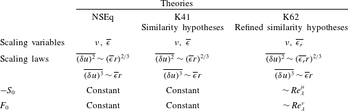
We now compare the NSEq-based analysis results with those of K41 and K62 (table 1). We observe that while K41 yields similar results to those obtained with the NSEq as
 $Re_{\unicode[STIX]{x1D706}}\rightarrow \infty$
, K62 leads to different results, with the exception of
 $\overline{(\unicode[STIX]{x1D6FF}u)^{3}}$
, which must comply with the
 $4/5$
law. It is interesting to note that in his attempt to ‘correct K41’ in K62, Kolmogorov accounts for large-scale fluctuations of
 $\unicode[STIX]{x1D716}$
originating from the inhomogeneity of the large scales, which he excluded in K41 in the first place. Also, Kolmogorov introduces the effects of large-scale inhomogeneity through phenomenological arguments in order to correct the two-thirds law, but, at the same time, uses his four-fifths law, which, as seen above, can only be correct when the large-scale inhomogeneities are non-existent. One can argue that Kolmogorov could have accounted for these large-scale effects in a natural, more rigorous and less empirical way by simply reintroducing the large-scale terms he neglected in the KH equation. We saw earlier that a power-law behaviour
 $\overline{(\unicode[STIX]{x1D6FF}u)^{n}}\sim r^{\unicode[STIX]{x1D701}_{n}}$
(
 $n=2,3$
and 4) in the scaling range is not compatible with the NSEq when these large-scale effects cannot be negligible and ignored. If one tries to fit (empirical) power-law expressions
 $r^{\unicode[STIX]{x1D701}_{n}}$
to the experimental and numerical data for
 $\overline{(\unicode[STIX]{x1D6FF}u)^{n}}$
over a narrow range of
 $r$
, usually identified as the scaling range, while the large-scale terms are not negligible in the KH equation, then one must not assume nor use
 $\overline{(\unicode[STIX]{x1D6FF}u)^{3}}=-(4/5)\overline{\unicode[STIX]{x1D716}}r$
.
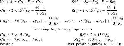
To better illustrate the comparison, we show in table 2 the results one obtains after substituting
 $S_{0}$
and
 $F_{0}$
from both K41 and K62 into (A 34) and (A 35) and letting
 $Re_{\unicode[STIX]{x1D706}}$
increase. While
 $S_{0}$
and
 $F_{0}$
for K41 comply with the NSEq, the expressions
 $-S_{0}\sim Re_{\unicode[STIX]{x1D706}}^{\unicode[STIX]{x1D707}}$
and
 $F_{0}\sim Re_{\unicode[STIX]{x1D706}}^{\unicode[STIX]{x1D708}}$
lead to the incongruous result that the left-hand sides of both (A 34) and (A 35) increase continuously with
 $Re_{\unicode[STIX]{x1D706}}$
whereas the right-hand sides approach a constant. This, however, is not surprising since scale invariance is assumed broken in K62.
Comparison of theoretical results. The
 $2/3$
law is obtained if one assumes that
 $S$
is constant in the inertial range. Both
 $\unicode[STIX]{x1D707}$
and
 $\unicode[STIX]{x1D708}$
are supposed to be positive numbers (
 $0<\unicode[STIX]{x1D707},\unicode[STIX]{x1D708}<1$
).

Testing the K41 and K62 predictions for the skewness and flatness factor of (
 $\unicode[STIX]{x2202}u/\unicode[STIX]{x2202}x$
) against the NSEq-based results.

A final remark is warranted before concluding this section. K41 is valid only for infinitely large
 $Re_{\unicode[STIX]{x1D706}}$
, and is not meant to apply at finite Reynolds numbers; likewise for K62. One can then argue that the variation of
 $S_{0}$
and
 $F_{0}$
observed at finite Reynolds numbers should not be interpreted as a ‘deviation from K41’. Strictly, one must compare K41 with any results (experimental or numerical) for which the conditions required by K41 (isotropy and infinitely large
 $Re_{\unicode[STIX]{x1D706}}$
) are satisfied. Only then can any variation observed between K41 and the results be considered as a departure from K41.
6 Comparison with measurements
Scale invariance for finite Reynolds number decaying HIT requires that the scaling Reynolds number remains constant during decay. Unfortunately, this cannot be tested experimentally since it is not possible to generate HIT in the laboratory. The laboratory flow which comes closest to decaying HIT is grid turbulence generated by a fluid flowing through a grid. After an initial increase, just downstream of the grid, the turbulent kinetic energy decreases with increasing distance,
 $x$
, downstream of the grid, leading to a decaying pseudo-HIT. However,
 $Re_{\unicode[STIX]{x1D706}}$
is observed to decrease with increasing
 $x$
, thus ruling out scale invariance, at least at all scales of motion. Scale invariance can be achieved only when the turbulent kinetic energy decays like
 $x^{-1}$
(Djenidi & Antonia Reference Djenidi and Antonia2015). A Similar observation can be made with regards to numerical simulations (direct and EDQNM) of decaying HIT. It appears that the prospect of testing any analytical developments of decaying HIT is rather grim. Nevertheless, some relatively recent results provide some encouragement. We start with the results of Antonia et al. (Reference Antonia, Djenidi and Danaila2014) which show that the Kolmogorov normalised velocity spectra collapse over the dissipative range in many decaying turbulent flows supporting the notion that similarity solutions for the small scales based on the Kolmogorov variables are valid when the effect of the large terms in (A 7) and (A 8) is negligible, i.e. when
 $Re_{\unicode[STIX]{x1D706}}$
is very large. In the dissipative range, equations (A 7) and (A 8) become (A 34) and (A 35) when normalised by Kolmogorov scales; the latter equations indicate that both
 $-S_{0}$
and
 $F_{0}$
become independent of
 $Re_{\unicode[STIX]{x1D706}}$
as
 $Re_{\unicode[STIX]{x1D706}}$
increases. Antonia et al. (Reference Antonia, Tang, Djenidi and Danaila2015), Tang et al. (Reference Tang, Antonia, Djenidi, Abe, Zhou., Danaila and Zhou2015a
,Reference Tang, Antonia, Djenidi and Zhou
c
), Antonia et al. (Reference Antonia, Djenidi, Danaila and Tang2017) and Tang et al. (Reference Tang, Antonia, Djenidi and Zhou2018) already reported the Reynolds number dependence of
 $-S_{0}$
and
 $F_{0}$
in several turbulent flows. These studies showed that, as
 $Re_{\unicode[STIX]{x1D706}}$
increases,
 $-S_{0}$
and
 $F_{0}$
first increase before approaching constant values. To illustrate this
 $Re_{\unicode[STIX]{x1D706}}$
-dependence, figure 1 shows the variations of
 $-S_{0}$
and
 $F_{0}$
with
 $Re_{\unicode[STIX]{x1D706}}$
along the axis in the far field of a plane jet; local isotropy is approximatively satisfied in this region of the flow. Both
 $-S_{0}$
and
 $F_{0}$
first increase before approaching constant values, in agreement with the predictions of (A 34) and (A 35). Note that
 $-S_{0}$
approaches a constant at a faster rate than
 $F_{0}$
, supporting the idea that the higher the order of the moment, the higher
 $Re_{\unicode[STIX]{x1D706}}$
must be for the finite Reynolds number effect to become negligible. Recent EDQNM numerical simulations for
 $Re_{\unicode[STIX]{x1D706}}$
up to
 $10^{5}$
(Meldi et al.
Reference Meldi, Djenidi and Antonia2018) support the results shown in figure 1 as well as the present analysis.
Dependence of
 $-S_{0}$
and
 $F_{0}$
on
 $Re_{\unicode[STIX]{x1D706}}$
in a plane jet. ▴, Antonia, Anselmet & Chambers (Reference Antonia, Anselmet and Chambers1986); ▾, Sreenivasan & Antonia (Reference Sreenivasan and Antonia1997); ●, Antonia et al. (Reference Antonia, Djenidi, Danaila and Tang2017). Blue symbols are reproduced from figure 4 of Tang et al. (Reference Tang, Antonia, Djenidi and Zhou2018) without identifying the data sources. The blue and red dashed lines correspond to magnitudes of 0.53 and 10, respectively.

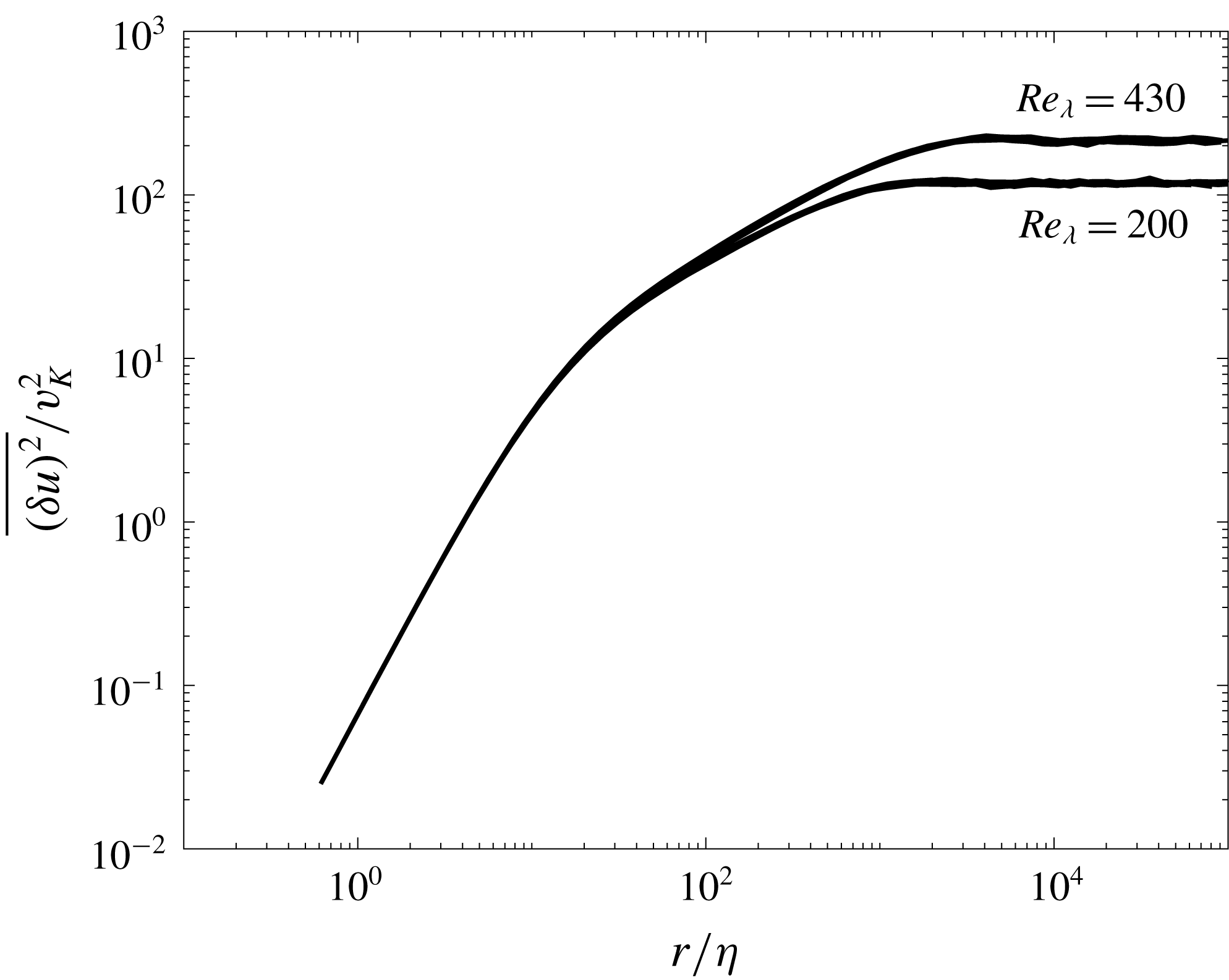
Distributions of Kolmogorov normalised
 $\overline{(\unicode[STIX]{x1D6FF}u)^{2}}$
on the centreline of a turbulent round jet for two
 $Re_{\unicode[STIX]{x1D706}}$
. For each
 $Re_{\unicode[STIX]{x1D706}}$
, several distributions along the jet axis over a range of positions between 30 and 60 times the jet nozzle diameter are reported.

Effect of the Reynolds number on the distributions of
 $\overline{(\unicode[STIX]{x1D6FF}u^{\ast })^{2}}$
in various flows normalised by
 $(\unicode[STIX]{x1D702},v_{K})$
(top) and
 $(u^{\prime },L)$
. Black lines: grid turbulence (Zhou & Antonia (Reference Zhou and Antonia2000),
 $Re_{\unicode[STIX]{x1D706}}=25$
–99); red lines: circular cylinder wake (Antonia, Zhou & Romano (Reference Antonia, Zhou and Romano2002),
 $Re_{\unicode[STIX]{x1D706}}=160$
–280); pink lines: plane jet (Antonia et al. (Reference Antonia, Djenidi, Danaila and Tang2017),
 $Re_{\unicode[STIX]{x1D706}}=550$
–1067); green lines: round jet (Xu, Antonia & Rajagopalan (Reference Xu, Antonia and Rajagopalan2001),
 $Re_{\unicode[STIX]{x1D706}}=235$
–545). The blue dashed line represents
 $r^{\ast 2}/15$
.

As stated above, scale invariance is not achieved in decaying grid turbulence. However, there are at least two cases where scale invariance is relatively well verified at finite Reynolds numbers: decaying turbulence on the centreline in the far fields of a round jet (Burattini, Antonia & Danaila Reference Burattini, Antonia and Danaila2005; Djenidi et al.
Reference Djenidi, Antonia, Lefeuvre and Lemay2015) and a cylinder wake (Tang et al.
Reference Tang, Antonia, Djenidi and Zhou2015b
). It was found that the distributions of
 $\overline{(\unicode[STIX]{x1D6FF}u)^{2}}$
collapsed very well at all scales when normalised using either (
 $\unicode[STIX]{x1D702}$
,
 $v_{K}$
) or (
 $u^{\prime }$
,
 $L$
). Figure 2, which displays Kolmogorov normalised distributions of
 $\overline{(\unicode[STIX]{x1D6FF}u)^{2}}$
at several positions along the centreline of a round jet from
 $30D$
to
 $60D$
(
 $D$
is the jet nozzle diameter) for two
 $Re_{\unicode[STIX]{x1D706}}$
(e.g. Djenidi et al.
Reference Djenidi, Antonia, Lefeuvre and Lemay2015), illustrates well this scale-invariance behaviour. The collapse at all scales for each
 $Re_{\unicode[STIX]{x1D706}}$
justifies the approach used in § 4 to derive the
 $n$
-thirds law, where no matching procedure was required. In accordance with the discussion in § 4, the two sets of data do not (and cannot) collapse, reflecting the Reynolds number dependence. To further illustrate this dependence, we show in figure 3 the distributions of
 $\overline{(\unicode[STIX]{x1D6FF}u)^{2}}$
normalised by
 $(\unicode[STIX]{x1D702},v_{K})$
and
 $(L,u^{\prime })$
for increasing
 $Re_{\unicode[STIX]{x1D706}}$
at a fixed position in different turbulent flows where local isotropy is satisfied approximately. There is a clear lack of collapse, even for a given turbulent flow, as
 $Re_{\unicode[STIX]{x1D706}}$
increases. For each flow, the collapse, when
 $\unicode[STIX]{x1D702}$
and
 $v_{K}$
are used, extends to larger separations as
 $Re_{\unicode[STIX]{x1D706}}$
increases. When the normalisation is by
 $L$
and
 $u^{\prime }$
, all the distributions come together when
 $r/L$
exceeds 1. This is as expected since
 $\overline{(\unicode[STIX]{x1D6FF}u)^{2}}/{u^{\prime }}^{2}$
must be equal to 2 when
 $r>L$
. The lack of collapse at all scales regardless of which normalisation is used reflects a lack of Reynolds number similarity, which states that any normalised distribution should be independent of the Reynolds number (e.g. Townsend Reference Townsend1956). The lack of such Reynolds number similarity is not, however, incompatible with scale invariance with respect to
 $x/D$
or more generally with
 $x$
, where the Reynolds number does not evolve with
 $x$
, at any given Reynolds number as seen in figure 2. It simply means that the constants of proportionality between scaling variables are Reynolds number dependent, as expressed by (2.7) and (2.8).
Distributions of
 $-\overline{(\unicode[STIX]{x1D6FF}u)^{3}}/(\overline{\unicode[STIX]{x1D716}}r)$
at
 $Re_{\unicode[STIX]{x1D706}}=72$
(▪),
 $144$
(●) and 2260 (♦) in grid turbulence (Gagne et al.
Reference Gagne, Castaing, Baudet and Malecot2004).

The
 $Re_{\unicode[STIX]{x1D706}}$
variation of the second term on the right-hand side of (3.15) (red curve) and the third term on the right-hand side of (3.16) (blue curve), divided by
 $r^{\ast }$
and
 $r^{\ast 4/3}$
, respectively, for
 $r=\unicode[STIX]{x1D706}$
in grid turbulence. The red curve has already been reported in Tang et al. (Reference Tang, Antonia, Djenidi, Danaila and Zhou2017) (see their figure 7).

Notice that
 $\overline{(\unicode[STIX]{x1D6FF}u^{\ast })^{2}}$
does not exhibit a scaling range where one can fit a power-law
 $r^{\unicode[STIX]{x1D701}_{n}}$
, which is consistent with our analysis in § 3.4. The lack of a scaling range is highlighted in figure 4 where we report distributions of
 $\overline{(\unicode[STIX]{x1D6FF}u)^{3}}/\overline{\unicode[STIX]{x1D716}}r$
for the grid turbulence data of Gagne et al. (Reference Gagne, Castaing, Baudet and Malecot2004) at
 $Re_{\unicode[STIX]{x1D706}}=72$
,
 $144$
and 2260 (the data for
 $Re_{\unicode[STIX]{x1D706}}=2260$
were obtained in the ONERA wind tunnel at Modane). The results of figure 4 show that while the maximum of (
 $\overline{(\unicode[STIX]{x1D6FF}u)^{3}}/\overline{\unicode[STIX]{x1D716}}r$
) approaches the value
 $4/5$
as
 $Re_{\unicode[STIX]{x1D706}}$
increases, there is a clear lack of a plateau, ruling out any existence of an inertial range, in support of the analysis of § 3.4: for
 $r^{\ast }$
beyond the dissipative range and as long as the large-scale terms in (3.15) are not zero (or equivalently
 $Re_{\unicode[STIX]{x1D706}}$
is not infinitely large),
 $\overline{(\unicode[STIX]{x1D6FF}u)^{3}}$
cannot vary proportionally to
 $r$
. The absence of a scaling range is attributed to the presence the large-scale terms in (3.15) and (3.16). To illustrate this, we calculated the last terms on the right-hand side of (3.15) and (3.16) for
 $r=\unicode[STIX]{x1D706}$
. We used an analytical expression for
 $\overline{(\unicode[STIX]{x1D6FF}u)^{2}}$
proposed and tested by Antonia & Burattini (Reference Antonia and Burattini2006) to compute
 $\overline{(\unicode[STIX]{x1D6FF}u)^{3}}$
,
 $\unicode[STIX]{x1D6E4}_{1}$
,
 $\unicode[STIX]{x1D6E4}_{2}$
,
 $\unicode[STIX]{x1D6E4}_{7}$
and
 $\unicode[STIX]{x1D6E4}_{8}$
to obtain smooth distributions. Before calculating
 $\unicode[STIX]{x1D6E4}_{7}$
and
 $\unicode[STIX]{x1D6E4}_{8}$
, we compared (not shown here) the calculated values of
 $\overline{(\unicode[STIX]{x1D6FF}u)^{3}}$
with the experimental data shown in figure 4. The close agreement we observed provided confidence for calculating
 $\unicode[STIX]{x1D6E4}_{7}$
and
 $\unicode[STIX]{x1D6E4}_{8}$
in this manner. Figure 5 displays the variation of the last term on the right-hand side of (3.15) and (3.16), divided by
 $r^{\ast }$
and
 $r^{\ast 4/3}$
, respectively. In agreement with the theoretical analysis, these terms decrease slowly with increasing
 $Re_{\unicode[STIX]{x1D706}}$
, highlighting the lingering effect of the large-scale motion responsible for the lack of power-law behaviour for
 $\overline{(\unicode[STIX]{x1D6FF}u)^{2}}$
,
 $\overline{(\unicode[STIX]{x1D6FF}u)^{3}}$
and
 $\overline{(\unicode[STIX]{x1D6FF}u)^{4}}$
. Interestingly, the rate of decrease of the magnitude of the large-scale terms with increasing
 $Re_{\unicode[STIX]{x1D706}}$
is slower in the transport equation for
 $\overline{(\unicode[STIX]{x1D6FF}u)^{3}}$
than in that for
 $\overline{(\unicode[STIX]{x1D6FF}u)^{2}}$
, implying that
 $\overline{(\unicode[STIX]{x1D6FF}u)^{3}}\sim r$
is approached at a faster rate than
 $\overline{(\unicode[STIX]{x1D6FF}u)^{4}}\sim r^{4/3}$
as
 $Re_{\unicode[STIX]{x1D706}}$
increases.
7 Concluding discussion
The scale-invariance property of the NSEq was exploited to investigate its consequences in finite Reynolds number HIT. The work expands and generalises in a significant manner that of Djenidi et al. (Reference Djenidi, Antonia and Danaila2017a
,Reference Djenidi, Danaila, Antonia and Tang
b
) who limited their analysis to self-preservation solutions when HIT evolves in time or space. The transport equations for the second- and third-order moments of the longitudinal velocity increment,
 $(\unicode[STIX]{x1D6FF}u)$
, have been considered. It is shown that:
(1) The scaling length and scaling velocity that leave self-preservation solutions and the equations of motion invariant are proportional to the length and velocity scales formed with
$\unicode[STIX]{x1D708}$
and
$\overline{\unicode[STIX]{x1D716}}$
(i.e. the Kolmogorov scales). Further, the scale-invariance property of the equations imposes that the constants of proportionality be equal to 1, indicating that the Kolmogorov scaling emerges as a natural consequence of scale invariance. Note that one can always normalise the equations of motion with any arbitrary scaling variables, other than Kolmogorov scales, derived from dimensional analysis; but these scales will not necessarily comply with the scale-invariance property of the equations.(2) When the Kolmogorov scales are used as the scaling variables, the equations and their solutions become approximately
$Re$
-independent for very large Reynolds numbers. For example, the skewness and flatness factor of the longitudinal velocity derivative are shown to become constant when
$Re_{\unicode[STIX]{x1D706}}$
increases to infinitely large values.(3) As a consequence of scale invariance, one can recover the
$n$
-thirds law (i.e.
$\overline{(\unicode[STIX]{x1D6FF}u)^{n}}\sim r^{n/3}$
) when
$Re_{\unicode[STIX]{x1D706}}\rightarrow \infty$
without resorting to the use of asymptotic matching expansions.


Comparison of the analytical results with measurements shows good agreement. In particular, the measurements confirm the absence of a power-law behaviour
 $\overline{(\unicode[STIX]{x1D6FF}u)^{n}}\sim r^{\unicode[STIX]{x1D701}_{n}}$
(at least for
 $n=2$
, 3 and 4). However, the trend shown by the measurements, in agreement with the analysis, is that
 $\overline{(\unicode[STIX]{x1D6FF}u)^{3}}\sim r$
is approached as
 $Re_{\unicode[STIX]{x1D706}}$
continues to increase. This is in agreement with the results of Antonia & Burattini (Reference Antonia and Burattini2006), Ishihara et al. (Reference Ishihara, Gotoh and Kaneda2009) and Tchoufag et al. (Reference Tchoufag, Sagaut and Cambon2012). Further, the measurements of the skewness and flatness factor of the longitudinal velocity derivative are shown, in agreement with the analysis, to become constant when
 $Re_{\unicode[STIX]{x1D706}}$
increases.
It is important to stress that the present analysis, which leads to K41 for an infinitely large Reynolds number, must not be interpreted as an attempt to derive or establish K41. Indeed, K41 is strictly valid as
 $Re_{\unicode[STIX]{x1D706}}\rightarrow \infty$
, whereas our analysis, which is independent of K41, holds for any
 $Re_{\unicode[STIX]{x1D706}}$
. It simply demonstrates the compliance of K41 with the NSEq under scale invariance when
 $Re_{\unicode[STIX]{x1D706}}$
is infinitely large, and that Kolmogorov’s first similarity hypothesis is achievable at finite
 $Re_{\unicode[STIX]{x1D706}}$
. It is in fact not too surprising that K41 complies with the NSEq since the former uses an exact property of the latter, namely the scale-invariance property. Certainly, since K41, or K62 for that matter, cannot realistically be tested due to the infinite Reynolds number requirement, it would be more productive and correct to test finite Reynolds number theoretical results, such as those presented here. In that regard, the present analytical results should be seen and used as ‘benchmark’ results against which phenomenological models can be tested and compared at finite Reynolds numbers (as done for example in tables 1 and 2).
Finally, the present theoretical framework could be extended to transport equations for
 $\overline{(\unicode[STIX]{x1D6FF}u)^{p}}$
with
 $p>3$
to investigate for example the Reynolds number behaviour of
 $\overline{(\unicode[STIX]{x1D6FF}u)^{p}}$
and
 $S_{p}=\overline{(\unicode[STIX]{x1D6FF}u)^{p}}/\overline{(\unicode[STIX]{x1D6FF}u)^{2}}^{p/2}$
.
Acknowledgements
The financial support of the Australian Research Council is acknowledged. S.L.T. wishes to acknowledge support given to him by NSFC through grant 11702074.
Appendix A
A.1 Equations of motion
Starting with the NSEq written at two separate and independent spatial points
 $x$
and
 $x^{\prime }$
, the transport equations for
 $\unicode[STIX]{x1D6FF}u_{2}$
(
 $\equiv \overline{(\unicode[STIX]{x1D6FF}u)^{2}}$
) and
 $\unicode[STIX]{x1D6FF}u_{3}$
(
 $\equiv \overline{(\unicode[STIX]{x1D6FF}u)^{3}}$
) for HIT can be expressed as (Danaila et al.
Reference Danaila, Anselmet, Zhou and Antonia1999)
 $$\begin{eqnarray}\frac{\unicode[STIX]{x2202}\unicode[STIX]{x1D6FF}u_{2}}{\unicode[STIX]{x2202}t}+\left(\frac{\unicode[STIX]{x2202}}{\unicode[STIX]{x2202}r}+\frac{4}{r}\right)\unicode[STIX]{x1D6FF}u_{3}=-4\overline{\unicode[STIX]{x1D716}}+6\unicode[STIX]{x1D708}\left\{\frac{\unicode[STIX]{x2202}^{2}}{\unicode[STIX]{x2202}r^{2}}+\frac{4}{r}\frac{\unicode[STIX]{x2202}}{\unicode[STIX]{x2202}r}\right\}\unicode[STIX]{x1D6FF}u_{2}\end{eqnarray}$$
and (Hill Reference Hill2001)
 $$\begin{eqnarray}\displaystyle & & \displaystyle \frac{\unicode[STIX]{x2202}\unicode[STIX]{x1D6FF}u_{3}}{\unicode[STIX]{x2202}t}+\left\{\left(\frac{\unicode[STIX]{x2202}}{\unicode[STIX]{x2202}r}+\frac{2}{r}\right)\unicode[STIX]{x1D6FF}u_{4}-\frac{6}{r}(\overline{(\unicode[STIX]{x1D6FF}u)^{2}(\unicode[STIX]{x1D6FF}v)^{2}})\right\}=-2\unicode[STIX]{x1D708}E_{111}\nonumber\\ \displaystyle & & \displaystyle \qquad +\,2\unicode[STIX]{x1D708}\left\{-\frac{4}{r^{2}}\unicode[STIX]{x1D6FF}u_{3}+\frac{4}{r}\frac{\unicode[STIX]{x2202}\unicode[STIX]{x1D6FF}u_{3}}{\unicode[STIX]{x2202}r}+\frac{\unicode[STIX]{x2202}^{2}\unicode[STIX]{x1D6FF}u_{3}}{\unicode[STIX]{x2202}r^{2}}\right\}-T_{111},\end{eqnarray}$$
where
 $\overline{\unicode[STIX]{x1D716}}=-(2/3)(\unicode[STIX]{x2202}\overline{u^{2}}/\unicode[STIX]{x2202}t)$
,
 $\unicode[STIX]{x1D6FF}u_{4}=\overline{(\unicode[STIX]{x1D6FF}u)^{4}}$
. Also,
 $T_{111}$
and
 $E_{111}$
are defined as
 $$\begin{eqnarray}\displaystyle & \displaystyle T_{111}=\frac{3}{\unicode[STIX]{x1D70C}}\overline{(\unicode[STIX]{x1D6FF}u)^{2}\left(\frac{\unicode[STIX]{x2202}\unicode[STIX]{x1D6FF}p}{\unicode[STIX]{x2202}X}\right)}, & \displaystyle\end{eqnarray}$$
 $$\begin{eqnarray}\displaystyle & \displaystyle E_{111}=\overline{(\unicode[STIX]{x1D6FF}u)\tilde{\unicode[STIX]{x1D716}}}, & \displaystyle\end{eqnarray}$$
where
 $\tilde{\unicode[STIX]{x1D716}}=3\{(\unicode[STIX]{x2202}u/\unicode[STIX]{x2202}x)^{2}+(\unicode[STIX]{x2202}u^{\prime }/\unicode[STIX]{x2202}x^{\prime })^{2}\}+3\{(\unicode[STIX]{x2202}u/\unicode[STIX]{x2202}y)^{2}+(\unicode[STIX]{x2202}u^{\prime }/\unicode[STIX]{x2202}y^{\prime })^{2}\}+3\{(\unicode[STIX]{x2202}u/\unicode[STIX]{x2202}z)^{2}+(\unicode[STIX]{x2202}u^{\prime }/\unicode[STIX]{x2202}z^{\prime })^{2}\}$
.
In the above equations and expressions we used the transformation
 $X=(x+x^{\prime })/2$
(e.g. Hill Reference Hill2001) and the fact that
 $\unicode[STIX]{x2202}u/\unicode[STIX]{x2202}x^{\prime }=\unicode[STIX]{x2202}u^{\prime }/\unicode[STIX]{x2202}x=0$
. The second term on the left-hand side of both (A 1) and (A 2) is the transport term. The first term on the right-hand side of (A 1) is the dissipation term whose counterpart in (A 2) is the first term on the right-hand side of that latter equation (the second and third bracketed terms were missing from the expression of
 $E_{111}$
in Djenidi et al.
Reference Djenidi, Antonia and Danaila2017a
). Since we are concerned with HIT only, we can write this term as
 $$\begin{eqnarray}E_{111}=6\overline{(\unicode[STIX]{x1D6FF}u)\tilde{\unicode[STIX]{x1D716}}_{HIT}},\end{eqnarray}$$
where
 $$\begin{eqnarray}\tilde{\unicode[STIX]{x1D716}}_{HIT}=\left(\frac{\unicode[STIX]{x2202}u}{\unicode[STIX]{x2202}x}\right)^{2}+2\left(\frac{\unicode[STIX]{x2202}u}{\unicode[STIX]{x2202}y}\right)^{2}.\end{eqnarray}$$
The last term and the second term on the right-hand side of (A 1) and (A 2), respectively, are the viscous terms. The term
 $T_{111}$
is the pressure source term and has no equivalent in (A 1) for HIT.
Equations (A 1) and (A 2) can be further developed in a more useful form. After some trivial manipulations, we have
 $$\begin{eqnarray}\unicode[STIX]{x1D6FF}u_{3}=6\unicode[STIX]{x1D708}\frac{\unicode[STIX]{x2202}\unicode[STIX]{x1D6FF}u_{2}}{\unicode[STIX]{x2202}r}-\frac{3}{r^{4}}\int _{0}^{r}s^{4}\frac{\unicode[STIX]{x2202}\unicode[STIX]{x1D6FF}u_{2}}{\unicode[STIX]{x2202}t}\,\text{d}s-\frac{4}{5}\overline{\unicode[STIX]{x1D716}}r,\end{eqnarray}$$
 $$\begin{eqnarray}\displaystyle \unicode[STIX]{x1D6FF}u_{4}=\frac{6}{r^{2}}\int _{0}^{r}s(\overline{(\unicode[STIX]{x1D6FF}u)^{2}(\unicode[STIX]{x1D6FF}v)^{2}})\,\text{d}s-\frac{1}{r^{2}}\int _{0}^{r}s^{2}T_{111}\,\text{d}s-\frac{2\unicode[STIX]{x1D708}}{r^{2}}\int _{0}^{r}s^{2}E_{111}\,\text{d}s & & \displaystyle \nonumber\\ \displaystyle +\frac{2\unicode[STIX]{x1D708}}{r^{2}}\int _{0}^{r}\left\{-4+4s\frac{\unicode[STIX]{x2202}}{\unicode[STIX]{x2202}s}+s^{2}\frac{\unicode[STIX]{x2202}^{2}}{\unicode[STIX]{x2202}s^{2}}\right\}\unicode[STIX]{x1D6FF}u_{3}\,\text{d}s-\frac{1}{r^{2}}\int _{0}^{r}s^{2}\frac{\unicode[STIX]{x2202}\unicode[STIX]{x1D6FF}u_{3}}{\unicode[STIX]{x2202}t}\,\text{d}s, & & \displaystyle\end{eqnarray}$$
where
 $s$
is a dummy variable of integration. In the majority of studies of small-scale turbulence, the term in (A 7) containing the integral is dropped on the basis that the Reynolds number is large enough to allow a net scale separation between large and small scales. With a few exceptions (Saffman Reference Saffman and Zabusky1968; Landau & Lifshitz Reference Landau and Lifshitz1987), it is mainly over the last two decades or so that the term was systematically ‘reintroduced’ (see also a derivation due to Novikov (Reference Novikov1965) based on the functional formulation of turbulence). Danaila et al. (Reference Danaila, Anselmet, Zhou and Antonia1999) derived (A 7) in the context of decaying grid turbulence for investigating the contributions of the large scales, represented by the integral term.
A.2 Self-preservation
We seek self-preservation solutions to (A 7) and (A 8) in the following forms:
 $$\begin{eqnarray}\displaystyle & \displaystyle \unicode[STIX]{x1D6FF}u_{2}=u_{2}^{2}(t)f(r^{\ast }) & \displaystyle\end{eqnarray}$$
 $$\begin{eqnarray}\displaystyle & \displaystyle \unicode[STIX]{x1D6FF}u_{3}=u_{3}^{3}(t)g(r^{\ast }) & \displaystyle\end{eqnarray}$$
 $$\begin{eqnarray}\displaystyle & \displaystyle \unicode[STIX]{x1D6FF}u_{4}=u_{2}^{4}(t)h(r^{\ast }) & \displaystyle\end{eqnarray}$$
 $$\begin{eqnarray}\displaystyle & \displaystyle \unicode[STIX]{x1D6FF}v_{2}=v_{2}^{2}(t)f_{v}(r^{\ast }) & \displaystyle\end{eqnarray}$$
 $$\begin{eqnarray}\displaystyle & \displaystyle \overline{(\unicode[STIX]{x1D6FF}u)^{2}(\unicode[STIX]{x1D6FF}v)^{2}}=u_{2}^{2}(t)v_{2}^{2}(t)f_{uv}(r^{\ast }) & \displaystyle\end{eqnarray}$$
 $$\begin{eqnarray}\displaystyle & \displaystyle T_{111}=\frac{u_{2}^{4}(t)}{l(t)}\tilde{T}_{111}(r^{\ast }) & \displaystyle\end{eqnarray}$$
 $$\begin{eqnarray}\displaystyle & \displaystyle E_{111}=\frac{u_{2}^{3}(t)}{l^{2}(t)}\tilde{E}_{111}(r^{\ast }), & \displaystyle\end{eqnarray}$$
where
 $r^{\ast }=r/l(t)$
;
 $l(t)$
,
 $u_{2}(t)$
,
 $u_{3}(t)$
and
 $v_{2}(t)$
are a length scale and velocity scaling functions to be determined while
 $f$
,
 $g$
,
 $h$
,
 $f_{v}$
,
 $f_{uv}$
,
 $\tilde{T}_{111}$
and
 $\tilde{E}_{111}$
are dimensionless functions of
 $r^{\ast }$
only. Note that
 $f$
and
 $h$
which appear in (A 9) and (A 11) are not to be confused with the correlation functions in the KH equation. For convenience, we hereafter drop the variable
 $t$
. We introduce the skewness and flatness factors
 $S$
(
 $\equiv \unicode[STIX]{x1D6FF}u_{3}/\unicode[STIX]{x1D6FF}u_{2}^{3/2}$
) and
 $F$
(
 $\equiv \unicode[STIX]{x1D6FF}u_{4}/\unicode[STIX]{x1D6FF}u_{2}^{2}$
) and the mixed flatness factor
 $F_{uv}$
(
 $\equiv \overline{(\unicode[STIX]{x1D6FF}u)^{2}(\unicode[STIX]{x1D6FF}v)^{2}}/(\unicode[STIX]{x1D6FF}u_{2})^{2}$
) as SP controlling parameters. We will focus our attention on complete self-preservation. In this case, all scales of motion (i.e.
 $0\leqslant r\leqslant \infty$
) must behave according to (A 9)–(A 15), which, after substitution in (A 7) and (A 8), lead to
 $$\begin{eqnarray}\displaystyle & & \displaystyle 6f^{\prime }(r^{\ast })-Re_{l}Sf(r^{\ast })^{3/2}-\frac{3l^{2}}{\unicode[STIX]{x1D708}u_{2}^{2}}\frac{\unicode[STIX]{x2202}u_{2}^{2}}{\unicode[STIX]{x2202}t}\frac{1}{r^{\ast 4}}\int _{0}^{r^{\ast }}s^{\ast 4}f(s^{\ast })\,\text{d}s^{\ast }\nonumber\\ \displaystyle & & \displaystyle \qquad +\,\frac{3}{\unicode[STIX]{x1D708}}l\frac{\unicode[STIX]{x2202}l}{\unicode[STIX]{x2202}t}\frac{1}{r^{\ast 4}}\int _{0}^{r^{\ast }}s^{\ast 5}f^{\prime }(s^{\ast })\,\text{d}s^{\ast }=\frac{4}{5}\overline{\unicode[STIX]{x1D716}}\frac{l^{2}}{\unicode[STIX]{x1D708}u_{2}^{2}}r^{\ast }\end{eqnarray}$$
and
 $$\begin{eqnarray}\displaystyle Re_{l}Ff^{2} & = & \displaystyle \frac{6Re_{l}}{r^{\ast 2}}\frac{v_{2}^{2}}{u_{2}^{2}}\int _{0}^{r^{\ast }}s^{\ast }F_{uv}f^{2}\,\text{d}s^{\ast }-\frac{Re_{l}}{r^{\ast 2}}\int _{0}^{r^{\ast }}s^{\ast 2}\tilde{T}_{111}\,\text{d}s^{\ast }-\frac{2}{r^{\ast 2}}\int _{0}^{r^{\ast }}s^{\ast 2}\tilde{E}_{111}\,\text{d}s^{\ast }\nonumber\\ \displaystyle & & \displaystyle +\,\frac{2}{r^{\ast 2}}\int _{0}^{r^{\ast }}\left\{-4+4s^{\ast }\frac{\unicode[STIX]{x2202}}{\unicode[STIX]{x2202}s^{\ast }}+s^{2\ast }\frac{\unicode[STIX]{x2202}^{2}}{\unicode[STIX]{x2202}s^{\ast 2}}\right\}Sf^{3/2}\,\text{d}s^{\ast }\nonumber\\ \displaystyle & & \displaystyle -\,\frac{l^{2}}{\unicode[STIX]{x1D708}u_{2}^{3}}\frac{\unicode[STIX]{x2202}u_{2}^{3}}{\unicode[STIX]{x2202}t}\frac{1}{r^{\ast 2}}\int _{0}^{r^{\ast }}s^{\ast 2}Sf^{3/2}\,\text{d}s^{\ast }+\frac{l}{\unicode[STIX]{x1D708}}\frac{\unicode[STIX]{x2202}l}{\unicode[STIX]{x2202}t}\frac{1}{r^{\ast 2}}\int _{0}^{r^{\ast }}s^{\ast 3}\frac{\unicode[STIX]{x2202}(Sf^{3/2})}{\unicode[STIX]{x2202}s^{\ast }}\,\text{d}s^{\ast }.\end{eqnarray}$$
Since
 $f(r^{\ast })$
is constant for large
 $r^{\ast }$
, the second term on the left-hand side of (A 16) varies like
 $r^{\ast }$
as
 $r^{\ast }\rightarrow \infty$
while the fourth term becomes constant. Similarly, the last three terms on the right-hand side of (A 17) become zero as
 $r^{\ast }\rightarrow \infty$
, as shown by the direct numerical simulation data of Gotoh & Nakano (Reference Gotoh and Nakano2003) (see also Hill (Reference Hill2001)). It is evident that, if SP were to be valid, equations (A 16) and (A 17) must share the same scaling parameters. Since the coefficients of the first term on the left-hand side of (A 16) and the third term on the right-hand side of (A 17) are constant, it follows that the SP constraints are
 $$\begin{eqnarray}Re_{l}=C_{1},\quad \frac{v_{2}^{2}}{u_{2}^{2}}=C_{1,a}\end{eqnarray}$$
 $$\begin{eqnarray}\displaystyle & \displaystyle \frac{l^{2}}{\unicode[STIX]{x1D708}u_{2}^{2}}\frac{\unicode[STIX]{x2202}u_{2}^{2}}{\unicode[STIX]{x2202}t}=C_{2} & \displaystyle\end{eqnarray}$$
 $$\begin{eqnarray}\displaystyle & \displaystyle \frac{l}{\unicode[STIX]{x1D708}}\frac{\unicode[STIX]{x2202}l}{\unicode[STIX]{x2202}t}=C_{3} & \displaystyle\end{eqnarray}$$
 $$\begin{eqnarray}\displaystyle & \displaystyle \frac{l^{2}}{\unicode[STIX]{x1D708}u_{2}^{3}}\frac{\unicode[STIX]{x2202}u_{2}^{3}}{\unicode[STIX]{x2202}t}=C_{4} & \displaystyle\end{eqnarray}$$
 $$\begin{eqnarray}\displaystyle & \displaystyle \frac{\overline{\unicode[STIX]{x1D716}}l^{2}}{\unicode[STIX]{x1D708}u_{2}^{2}}=C_{5}, & \displaystyle\end{eqnarray}$$
where
 $Re_{l}=u_{2}l/\unicode[STIX]{x1D708}$
is a scaling Reynolds number. Note that
 $(l^{2}/\unicode[STIX]{x1D708}u_{2}^{2})(\unicode[STIX]{x2202}u_{2}^{2}/\unicode[STIX]{x2202}t)=2(l^{2}/\unicode[STIX]{x1D708}u_{2})(\unicode[STIX]{x2202}u_{2}/\unicode[STIX]{x2202}t)$
and
 $l^{2}/\unicode[STIX]{x1D708}u_{2}^{3}(\unicode[STIX]{x2202}u_{2}^{3}/\unicode[STIX]{x2202}t)=3(l^{2}/\unicode[STIX]{x1D708}u_{2})(\unicode[STIX]{x2202}u_{2}/\unicode[STIX]{x2202}t)$
then
 $C_{4}=(3/2)C_{2}$
. It can also be shown that using the definition of
 $Re_{l}$
with both expressions (A 19) and (A 20) yields
 $C_{3}=-(1/2)C_{2}$
. The above constraints, i.e.
 $C_{1}$
,
 $C_{1,a}$
,
 $C_{2}$
,
 $C_{3}$
,
 $C_{4}$
and
 $C_{5}$
are independent of
 $t$
, apply for all separations
 $r^{\ast }$
while the numerical values of the constants depend on the scaling variables.
Rather than imposing/selecting an arbitrary pair of length and velocity scales which must satisfy (A 18)–(A 22) (i.e.
 $l\sim u_{2}^{-1}$
) one can determine the expressions of the scaling variables which not only are compliant with the scale-invariance constraints but also ensure that the normalised solutions to (A 7) and (A 8) remain scale-invariant. Following Djenidi et al. (Reference Djenidi, Antonia and Danaila2017a
), we combine the first expression of (A 18) with (A 22) and, using the definition of
 $Re_{l}$
, we obtain
 $$\begin{eqnarray}l=(\sqrt{C_{5}}C_{1})^{1/2}\left(\frac{\unicode[STIX]{x1D708}^{3}}{\overline{\unicode[STIX]{x1D716}}}\right)^{1/4}.\end{eqnarray}$$
Now, substituting (A 23) into (A 22) leads to
 $$\begin{eqnarray}u_{2}=\left(\frac{C_{1}}{\sqrt{C_{5}}}\right)^{1/2}\left(\unicode[STIX]{x1D708}\overline{\unicode[STIX]{x1D716}}\right)^{1/4}.\end{eqnarray}$$
A.3 Analytical expression for
$S$
and
$F$


Analytical expressions for
 $S$
and
 $F$
, first developed by Djenidi et al. (Reference Djenidi, Antonia and Danaila2017a
,Reference Djenidi, Danaila, Antonia and Tang
b
), are written as follows:
 $$\begin{eqnarray}\displaystyle & \displaystyle -S(r^{\ast })=-6\frac{f^{-3/2}f^{\prime }}{Re_{l}}+\frac{f^{-3/2}}{Re_{l}}\left\{\frac{4}{5}C_{5}r^{\ast }+\frac{3}{r^{\ast 4}}C_{2}(\unicode[STIX]{x1D6E4}_{1}+\frac{1}{2}\unicode[STIX]{x1D6E4}_{2})\right\}, & \displaystyle\end{eqnarray}$$
 $$\begin{eqnarray}\displaystyle & \displaystyle F(r^{\ast })=6f^{-2}\unicode[STIX]{x1D6E4}_{3}-f^{-2}\unicode[STIX]{x1D6E4}_{4}+\frac{f^{-2}}{Re_{l}}\left\{2\unicode[STIX]{x1D6E4}_{5}+2\unicode[STIX]{x1D6E4}_{6}-\frac{C_{2}}{2}(3\unicode[STIX]{x1D6E4}_{7}+\unicode[STIX]{x1D6E4}_{8})\right\}, & \displaystyle\end{eqnarray}$$
where
 $$\begin{eqnarray}\displaystyle \left.\begin{array}{@{}c@{}}\unicode[STIX]{x1D6E4}_{1}=\int _{0}^{r^{\ast }}s^{\ast 4}f(s^{\ast })\,\text{d}s^{\ast },\quad \unicode[STIX]{x1D6E4}_{2}=\int _{0}^{r^{\ast }}s^{\ast 5}f^{\prime }(s^{\ast })\,\text{d}s^{\ast },\\ \unicode[STIX]{x1D6E4}_{3}=\frac{1}{r^{\ast 2}}\int _{0}^{r^{\ast }}s^{\ast }F_{uv}f^{2}\,\text{d}s^{\ast },\quad \unicode[STIX]{x1D6E4}_{4}=\frac{1}{r^{\ast 2}}\int _{0}^{r^{\ast }}s^{\ast 2}\tilde{T}_{111}\,\text{d}s^{\ast },\\ \unicode[STIX]{x1D6E4}_{5}=\frac{1}{r^{\ast 2}}\int _{0}^{r^{\ast }}s^{\ast 2}\tilde{E}_{111}\,\text{d}s^{\ast },\quad \unicode[STIX]{x1D6E4}_{6}=\frac{1}{r^{\ast 2}}\int _{0}^{r^{\ast }}\left\{-4+4s^{\ast }\frac{\unicode[STIX]{x2202}}{\unicode[STIX]{x2202}s^{\ast }}+s^{\ast 2}\frac{\unicode[STIX]{x2202}^{2}}{\unicode[STIX]{x2202}s^{\ast 2}}\right\}Sf^{3/2}\,\text{d}s^{\ast },\\ \unicode[STIX]{x1D6E4}_{7}=\frac{1}{r^{\ast 2}}\int _{0}^{r^{\ast }}s^{\ast 2}Sf^{3/2}\,\text{d}s^{\ast },\quad \unicode[STIX]{x1D6E4}_{8}=\frac{1}{r^{\ast 2}}\int _{0}^{r^{\ast }}s^{\ast 3}\frac{\unicode[STIX]{x2202}(Sf^{3/2})}{\unicode[STIX]{x2202}s^{\ast }}\,\text{d}s^{\ast }.\end{array}\right\} & & \displaystyle\end{eqnarray}$$
A.4
$S$
and
$F$
in the limit
$R_{\unicode[STIX]{x1D706}}\rightarrow 0$


Expanding
 $f(r^{\ast })$
around
 $r^{\ast }=0$
with a Taylor series expansion to order four yields
 $$\begin{eqnarray}f(r^{\ast })\simeq \unicode[STIX]{x1D6FC}r^{\ast 2}-{\textstyle \frac{1}{12}}\unicode[STIX]{x1D6FD}r^{\ast 4},\end{eqnarray}$$
where
 $\unicode[STIX]{x1D6FC}=l^{2}/u_{2}^{2}\overline{(\unicode[STIX]{x2202}u/\unicode[STIX]{x2202}x)^{2}}$
and
 $\unicode[STIX]{x1D6FD}=l^{4}/u_{2}^{2}\overline{(\unicode[STIX]{x2202}^{2}u/\unicode[STIX]{x2202}x^{2})^{2}}$
are constant and whose values depend on the choice of
 $l$
and
 $u_{2}$
. Substituting (A 28) into (A 25) and (A 26), using (3.6) and equating terms in
 $r^{\ast 3}$
and
 $r^{\ast 4}$
, respectively, in these equations yields
 $$\begin{eqnarray}-S_{0}=2\frac{\unicode[STIX]{x1D6FD}\unicode[STIX]{x1D6FC}^{-3/2}}{Re_{l}}+\frac{6C_{2}}{7}\frac{\unicode[STIX]{x1D6FC}^{-1/2}}{Re_{l}}\end{eqnarray}$$
and
 $$\begin{eqnarray}\displaystyle F_{0}=F_{uv,0}-\frac{1}{2}\unicode[STIX]{x1D6FE}_{1}\unicode[STIX]{x1D6FC}^{-2}+\frac{1}{Re_{l}}\left\{2\unicode[STIX]{x1D6FE}_{2}\unicode[STIX]{x1D6FC}^{-2}-\frac{1}{2}C_{2}S_{0}\unicode[STIX]{x1D6FC}^{-1/2}\right\}\!, & & \displaystyle\end{eqnarray}$$
where
 $\unicode[STIX]{x1D6FE}_{1}=l^{4}/u_{2}^{4}\overline{(\unicode[STIX]{x2202}u/\unicode[STIX]{x2202}x)^{2}(\unicode[STIX]{x2202}^{2}p/\unicode[STIX]{x2202}x^{2})}$
and
 $\unicode[STIX]{x1D6FE}_{2}=(l^{5}/u_{2}^{3})\overline{\widetilde{\unicode[STIX]{x1D716}_{eq}}(\unicode[STIX]{x2202}^{3}u/\unicode[STIX]{x2202}x^{3})}$
with
 $\widetilde{\unicode[STIX]{x1D716}_{eq}}=(7/12)(\unicode[STIX]{x2202}u/\unicode[STIX]{x2202}x)^{2}-(1/3)(\unicode[STIX]{x2202}u/\unicode[STIX]{x2202}y)^{2}$
. Note that the expression of
 $\widetilde{\unicode[STIX]{x1D716}_{eq}}$
combines terms from both
 $\unicode[STIX]{x1D6E4}_{5}$
and
 $\unicode[STIX]{x1D6E4}_{6}$
.
As seen in § 2, these equations can be scale-invariant only when
 $l=(\unicode[STIX]{x1D708}^{3}/\overline{\unicode[STIX]{x1D716}})^{1/4}$
and
 $u_{2}=(\unicode[STIX]{x1D708}\overline{\unicode[STIX]{x1D716}})^{1/4}$
, which we now use (such a scaling will be used hereafter unless otherwise noted). This leads to
 $$\begin{eqnarray}-S_{0}=2\unicode[STIX]{x1D6FD}_{K}\unicode[STIX]{x1D6FC}_{K}^{-3/2}+\frac{6C_{2,K}}{7}\unicode[STIX]{x1D6FC}_{K}^{-1/2}\end{eqnarray}$$
and
 $$\begin{eqnarray}\displaystyle F_{0}=F_{uv,0}-{\textstyle \frac{1}{2}}\unicode[STIX]{x1D6FE}_{1,K}\unicode[STIX]{x1D6FC}_{K}^{-2}+2\unicode[STIX]{x1D6FE}_{2,K}\unicode[STIX]{x1D6FC}_{K}^{-2}-{\textstyle \frac{1}{2}}C_{2,K}S_{0}\unicode[STIX]{x1D6FC}_{K}^{-1/2}. & & \displaystyle\end{eqnarray}$$
Further,
 $$\begin{eqnarray}\unicode[STIX]{x1D6FC}_{K}=\frac{\unicode[STIX]{x1D702}^{2}}{v_{K}^{2}}\overline{\left(\frac{\unicode[STIX]{x2202}u}{\unicode[STIX]{x2202}x}\right)^{2}}=\frac{\unicode[STIX]{x1D702}^{2}}{v_{K}^{2}}\frac{\overline{\unicode[STIX]{x1D716}}}{15\unicode[STIX]{x1D708}}=\frac{C_{5,K}}{15}=\frac{1}{15},\end{eqnarray}$$
where we use the constraints (A 18)–(A 22) and (A 23) to relate
 $\unicode[STIX]{x1D702}$
to
 $\unicode[STIX]{x1D706}$
, and the constraint (A 24) to relate
 $v_{K}$
to
 $u^{\prime }$
. Also, we use the fact that scale invariance requires
 $Re_{\unicode[STIX]{x1D706}}$
to be constant (when
 $\unicode[STIX]{x1D708}\neq 0$
). Using (3.3), we can now write
 $S_{0}$
as
 $$\begin{eqnarray}-S_{0}=2\times 15^{3/2}\unicode[STIX]{x1D6FD}_{K}-\frac{60}{7}\frac{1}{Re_{\unicode[STIX]{x1D706}}}.\end{eqnarray}$$
To obtain an expression for
 $F_{0}$
, we first use the result
 $F_{uv,0}\simeq (17/20)F_{0}$
obtained by Djenidi et al. (Reference Djenidi, Danaila, Antonia and Tang2017b
). We then substitute (A 33) and (3.3) into (A 32) and after some trivial manipulations we obtain
 $$\begin{eqnarray}F_{0}=-750[\unicode[STIX]{x1D6FE}_{1,K}-4\unicode[STIX]{x1D6FE}_{2,K}]-\frac{100}{3}\frac{S_{0}}{Re_{\unicode[STIX]{x1D706}}}.\end{eqnarray}$$
Since
 $15^{3/2}\unicode[STIX]{x1D6FD}_{K}=G/Re_{\unicode[STIX]{x1D706}}$
(
 $G=\overline{(u^{2})}(\!\overline{(\unicode[STIX]{x2202}^{2}u/\unicode[STIX]{x2202}x^{2})^{2}}/\overline{\unicode[STIX]{x2202}u/\unicode[STIX]{x2202}x)^{2}}^{2}$
), we immediately note that (A 34) is the same expression as first obtained by Batchelor & Townsend (Reference Batchelor and Townsend1947) (see their expression (4.3)) when the decay exponent
 $n=-1$
. This is not surprising since when
 $r\rightarrow 0$
, the transport equation (A 7) becomes the transport equation for
 $\overline{\unicode[STIX]{x1D716}}$
and, for HIT,
 $\overline{\unicode[STIX]{x1D716}}=\unicode[STIX]{x1D708}\overline{\unicode[STIX]{x1D714}^{2}}$
, where
 $\overline{\unicode[STIX]{x1D714}^{2}}=\overline{\unicode[STIX]{x1D714}_{i}\unicode[STIX]{x1D714}_{i}}$
with
 $\unicode[STIX]{x1D714}_{i}$
being the vorticity components.
A.5 Moments of
$\unicode[STIX]{x2202}u/\unicode[STIX]{x2202}x$

The constancy of both
 $S_{0}$
and
 $F_{0}$
can be also shown as follows. For very small values of
 $r^{\ast }$
, using a Taylor series expansion around
 $r^{\ast }\simeq 0$
, we can write
 $$\begin{eqnarray}\unicode[STIX]{x1D6FF}u_{m}=u_{2}^{m}(t)f_{m}(r^{\ast })\sim r^{\ast m}l^{m}\overline{\left(\frac{\unicode[STIX]{x2202}u}{\unicode[STIX]{x2202}x}\right)^{m}},\end{eqnarray}$$
which leads to
 $$\begin{eqnarray}\overline{\left(\frac{\unicode[STIX]{x2202}u}{\unicode[STIX]{x2202}x}\right)^{m}}\sim \frac{u_{2}^{m}(t)f_{m}(r^{\ast })}{r^{\ast m}l^{m}}.\end{eqnarray}$$
Since
 $\unicode[STIX]{x1D702}$
and
 $v_{K}$
are the correct scaling variables (under scale invariance), we can use them in (A 37), which simplifies to
 $$\begin{eqnarray}\overline{\left(\frac{\unicode[STIX]{x2202}u}{\unicode[STIX]{x2202}x}\right)^{m}}\sim \left(\frac{v_{K}}{\unicode[STIX]{x1D702}}\right)^{m}\!,\end{eqnarray}$$
given that
 $f_{m}(r^{\ast })\sim (1/15)^{m}r^{\ast m}$
. Finally, using the definitions of
 $\unicode[STIX]{x1D702}$
and
 $v_{K}$
yields
 $$\begin{eqnarray}\overline{\left(\frac{\unicode[STIX]{x2202}u}{\unicode[STIX]{x2202}x}\right)^{m}}\sim \left(\frac{\overline{\unicode[STIX]{x1D716}}}{\unicode[STIX]{x1D708}}\right)^{\frac{m}{2}}\!.\end{eqnarray}$$
Expressions (A 38) or (A 39) show that the ratio
 $\overline{(\unicode[STIX]{x2202}u/\unicode[STIX]{x2202}x)^{m}}/\overline{(\unicode[STIX]{x2202}u/\unicode[STIX]{x2202}x)^{2}}^{m/2}$
(
 $m\geqslant 2$
) is an absolute constant, which shows that for
 $m=3$
and 4,
 $S_{0}$
and
 $F_{0}$
should approach constant values as
 $Re_{\unicode[STIX]{x1D706}}$
increases. Batchelor (Reference Batchelor1947) was first to arrive at (A 39). However, there is an important difference between Batchelor’s approach and ours. Batchelor introduced
 $\unicode[STIX]{x1D702}$
and
 $v_{K}$
as the scaling variables. We first show, starting with the equations of motion, that
 $\unicode[STIX]{x1D702}$
and
 $v_{K}$
are the correct scaling variables before using them.
A.6 The minus fifth-thirds law
We follow Gamard & George (Reference Gamard and George2000) up to the point where they write their low- and high-wavenumber normalised spectra
 $F_{L}$
and
 $F_{H}$
, respectively:
 $$\begin{eqnarray}F_{L}(k^{+})=\frac{E(k,t)}{{u^{\prime }}^{2}L}\end{eqnarray}$$
and
 $$\begin{eqnarray}F_{H}(k^{\ast })=\frac{E(k,t)}{u_{K}^{2}\unicode[STIX]{x1D702}},\end{eqnarray}$$
where
 $k^{+}=kL$
and
 $k^{\ast }=k\unicode[STIX]{x1D702}$
. Note that we also followed Gamard & George (Reference Gamard and George2000) in using
 $u^{\prime }$
and
 $L$
as the large-scale variables. Since scale invariance implies that the Reynolds number is constant and we want to consider the case of infinitely large Reynolds number, then both
 $F_{L}$
and
 $F_{H}$
should be explicitly independent of the Reynolds number. Noting that
 $F_{L}$
and
 $F_{H}$
represent exactly the same spectrum, we can write
 $$\begin{eqnarray}F_{H}(k^{\ast })=\frac{{u^{\prime }}^{2}L}{u_{K}^{2}\unicode[STIX]{x1D702}}F_{L}(k^{+}).\end{eqnarray}$$
Using (2.7) and (2.8) (scale invariance is achieved at scales ranging from
 $\unicode[STIX]{x1D702}$
to
 $L$
) yields
 $$\begin{eqnarray}F_{H}(k^{\ast })=\frac{Re_{L}^{5/4}}{C_{\unicode[STIX]{x1D716}}^{1/2}}F_{L}(k^{\ast }Re_{L}^{3/4}C_{\unicode[STIX]{x1D716}}^{1/4}).\end{eqnarray}$$
As for the structure function, equation (A 43) can be an identity if both
 $F_{H}$
and
 $F_{L}$
vary like
 $x^{n}$
. Substituting this form in (A 43) leads to
 $$\begin{eqnarray}k^{\ast n}Re_{L}^{-5/4}C_{\unicode[STIX]{x1D716}}^{1/2}=(k^{\ast }Re_{L}^{3/4}C_{\unicode[STIX]{x1D716}}^{1/4})^{n},\end{eqnarray}$$
which yields
 $n=-5/3$
. This leads to
 $$\begin{eqnarray}k^{\ast -5/3}=k^{\ast -5/3}C_{\unicode[STIX]{x1D716}}^{-2/3},\end{eqnarray}$$
so that
 $C_{\unicode[STIX]{x1D716}}=1$
. Notice the similarity between (4.5) and (A 45) when
 $n$
is equal to 2 in the former expression. The approach is in fact quite similar to that used by Tennekes & Lumley (Reference Tennekes and Lumley1975), but with one important difference. Those authors, who do not assume scale invariance at all scales, need to introduce the empirical relation
 $kL=Re_{L}^{n}$
, with
 $n$
to be determined by matching
 $F_{L}$
and
 $F_{H}$
. This relation allows them to write
 $k^{\ast }=kL(\unicode[STIX]{x1D702}/L)=Re_{L}^{n}(\unicode[STIX]{x1D702}/L)$
. They finally use
 $(\unicode[STIX]{x1D702}/L)\sim Re_{L}^{-3/4}$
, which according to (2.7) implies that
 $C_{\unicode[STIX]{x1D716}}=\text{const}$
. Thus, writing
 $k^{\ast }\sim Re_{L}^{n-3/4}$
imposes
 $0<n<1$
so that
 $k\unicode[STIX]{x1D702}\rightarrow 0$
and
 $kL\rightarrow \infty$
simultaneously when
 $Re_{L}\rightarrow \infty$
, thus allowing
 $F_{L}$
and
 $F_{H}$
to be matched. Gamard & George (Reference Gamard and George2000) use the same strategy. Since in our analysis, which is the same as that used for the structure function, scale invariance applies at all scales of motion, we do not need to stretch the range of validity of
 $F_{L}$
and
 $F_{H}$
nor perform a matching.