








1. Introduction
Since its commissioning at the National Ignition Facility (NIF), the Magnetic Recoil Spectrometer (MRS) has been routinely used to measure neutron spectra from deuterium–tritium (DT) implosions (Frenje et al. Reference Frenje2010; Frenje Reference Frenje2020). These measurements have supported a wide range of inertial confinement fusion (ICF) experiments (Smalyuk et al. Reference Smalyuk2014; Lindl et al. Reference Lindl, Landen and Edwards2014; Zylstra et al. Reference Zylstra2021), including recent campaigns leading to ignition (Abu-Shawareb et al. Reference Abu-Shawareb2022).
As seen in figure 1, the MRS consists of a deuterated polyethylene (
 $\mathrm{CD_2}$
) foil, a focusing magnet and an array of CR-39 detectors (Frenje et al. Reference Frenje2010; Casey et al. Reference Casey2013). The MRS operates as follows: neutrons are converted to deuterons via neutron–deuteron elastic scattering in the
 $\mathrm{CD_2}$
foil. Forward-scattered deuterons are selected by the magnet aperture, focused and dispersed onto CR-39 detectors according to their energy. Using the mapping between position and energy, the deuteron spectrum is measured. The spectrum is analysed using a forward-fit technique, where a model neutron spectrum is convolved with the MRS response function and iteratively adjusted until a match to the measured deuteron spectrum is found. From the best-fit model, the neutron yield (
 $Y_n$
), apparent ion temperature (
 $T_i$
) and areal density (
 $\rho R$
) are extracted.
Schematic of the MRS at the NIF. There is a tantalum blast shield placed in front the foil to block debris and X-rays from the implosion. The the top-right panel shows the observed modulated deuteron spectrum (red) relative to the response matrix fit (blue) for shot N240504-001. In the CR-39 scan image, the vertical axis corresponds to the non-dispersion direction and the horizontal axis represents the dispersion (energy) direction. The greyscale represents the number of deuteron tracks in each bin, with more white corresponding to more tracks.

Figure 1. Long description
A schematic of the Magnetic Recoil Spectrometer setup and deuteron energy measurement. The diagram shows an indirect drive system generating neutrons that pass through a tantalum blast shield and interact with a CD2 foil, producing recoil deuterons. These deuterons are then directed through a magnet and detected by CR-39 detectors labeled W1 to W9. The top-right panel displays a graph of deuteron count versus deuteron energy, with the observed modulated deuteron spectrum in red and the response matrix fit in blue. The inset shows a CR-39 scan image where the vertical axis corresponds to the non-dispersion direction and the horizontal axis represents the dispersion (energy) direction. The greyscale in the scan image indicates the number of deuteron tracks, with more white corresponding to more tracks.
Unexpected energy modulations in the MRS deuteron spectra have been observed in several high-yield NIF experiments
 $(Y_n \sim 10^{16}{-}10^{18})$
. The inset of figure 1 shows the deuteron spectrum from shot N240504-001, where the effect of modulation is the most visible. These modulations may introduce additional uncertainties to the inferred performance metrics
 $(Y_n, T_i, \rho R)$
, and the significance of these is investigated in this paper. As the MRS is upgraded to support higher yields
 $Y_n \gtrsim 10^{18}$
(Gatu Johnson et al. Reference Gatu Johnson2022), understanding the causes of energy modulations and mitigating their impact become increasingly important.
Proton-energy modulations have been observed in intense laser–matter interaction experiments (Hicks et al. Reference Hicks2001; Allen et al. Reference Allen2003; Busch et al. Reference Busch, Shiryaev, Ter-Avetisyan, Schnürer, Nickles and Sandner2004). The first reported observation likely comes from the charged particle spectrometer at the OMEGA facility, where oscillations were seen (Hicks et al. Reference Hicks2001). Based on the modulation period, Hicks et al. speculated that these structures result from ion-acoustic perturbations of an expanding plasma. Similar modulations have also been observed in target normal sheath acceleration experiments (Allen et al. Reference Allen2003; Busch et al. Reference Busch, Shiryaev, Ter-Avetisyan, Schnürer, Nickles and Sandner2004). Using particle-in-cell (PIC) simulations, Busch et al. (Reference Busch, Shiryaev, Ter-Avetisyan, Schnürer, Nickles and Sandner2004) attribute modulations to the presence of a two-temperature electron distribution, whereas Allen et al. (Reference Allen2003) suggest they arise from the presence of multiple heavy-ion species in an expanding plasma.
Ion-energy modulations have also been studied through the lens of kinetic instabilities under different plasma conditions. Tikhonchuk et al. (Reference Tikhonchuk, Andreev, Bochkarev and Bychenkov2005) proposed that a two-species plasma expansion can drive a two-stream instability (TSI), leading to energy and density modulations. Using PIC simulations under simplified ICF conditions (
 $n \sim 10^{22} \,{\mathrm{cm}^{-3}}$
,
 $T_e \sim 3$
keV), Lv et al. (Reference Lv2023) reproduced ion-energy oscillations reminiscent of past observations (Hicks et al. Reference Hicks2001). Fourier analysis of the electric field confirms that these oscillations originate from the ion-acoustic instability induced by the relative motion between counter-streaming ion species. Similar modulations have also been reported under non-ICF plasma conditions (
 $n \sim 10^{11} \,{\mathrm{cm}^{-3}}$
,
 $T_e \sim 10$
eV). For instance, Hui et al. (Reference Hui, Hu, Zhao, Cheng, Mei and Wang2019) performed three-dimensional PIC simulations of a mono-energetic proton beam propagating through a uniform plasma. They found that the initial energy peak evolves into two and later three peaks due to the TSI.
In this work, a combination of experimental data and simulations is used to constrain the foil conditions. Based on the estimated conditions, energy modulations are likely caused by the TSI driven by fast deuterons streaming through background electrons. Particle-in-cell simulations reasonably reproduce the observed energy modulations and show a linear scaling with the deuteron-to-electron density ratio (
 $n_d/n_e$
), which is stronger at higher yields. Synthetic spectra show negligible impact on MRS-inferred quantities at the current yields
 $Y_n\sim 10^{17}{-}10^{18}$
. However, the effect of modulations is expected to be significant at higher yields, which can be mitigated by placing the foil directly at the MRS.
This rest of this paper is organised as follows. Section 2 outlines the experimental conditions related to neutron–foil interactions and electron sources. In § 3, analytic theory is used to identify the TSI as the mechanism behind the observed energy modulations. Sections 4 and 5 present PIC simulations of shot N240504-001, where the pronounced modulations provide a clear basis for comparison. This is followed by a density scan to generalise the analysis beyond the simulated case. Section 6 concludes with a synthetic data study and briefly discusses potential mitigation strategies.
2. Experimental conditions
2.1. Neutron–foil interactions
Near peak convergence of the fuel, DT fusion in the hotspot produces energetic neutrons (14.1 MeV). Their energy spectrum is Doppler-broadened by the ion temperature
 $T_i$
, resulting in primary neutrons (
 $13{-}15$
MeV). Depending on
 $\rho R$
, a fraction of these neutrons scatter off fuel ions and lose energy, producing down-scattered neutrons (
 $10{-}12$
MeV) (Frenje et al. Reference Frenje2013).
Recoil deuterons are generated via neutron–deuteron elastic scattering in a
 $\mathrm{CD_2}$
foil located 26 cm from the target chamber centre (TCC). By conservation of momentum and energy, the deuteron energy
 $E_d$
is given by
 \begin{align} E_d = \frac {8}{9} E_n \cos ^2{\theta _{\text{lab}}}, \end{align}
where
 $E_n$
is the incident neutron energy and
 $\theta _{\text{lab}}$
is the laboratory scattering angle (Frenje et al. Reference Frenje2013). The differential distribution of
 $\theta _{\text{lab}}$
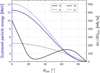
is extracted from the nuclear data repository ENDF (Brown et al. Reference Brown2018). Figure 2 displays the deuteron energy and angular distribution as a function of
 $\theta _{\text{lab}}$
for
 $E_n=14.1$
MeV. Due to the location and geometry of the magnet aperture relative to the foil, only forward-scattered deuterons (
 $\theta _{\text{lab}}\sim 0$
) are selected by the MRS. The spectral shape of these aperture-selected deuterons depends on the MRS response function, which was previously simulated by Casey et al. (Reference Casey2013) using the multi-physics code Geant4 (Agostinelli et al. Reference Agostinelli2003; Allison et al. Reference Allison2006, Reference Allison2016).
Scattered particle energy (blue) and angular distribution (black) as a function of
 $\theta _{\text{lab}}$
for deuterons (solid) and protons (dotted). The MRS aperture selects particles with
 $\theta _{\text{lab}} \sim 0$
.

Neutron–foil interactions can produce a range of other charged particles in addition to deuterons. To characterise the particle output, Geant4 simulations are performed, where an isotropic neutron source is placed 26 cm from a
 $\mathrm{CD_2}$
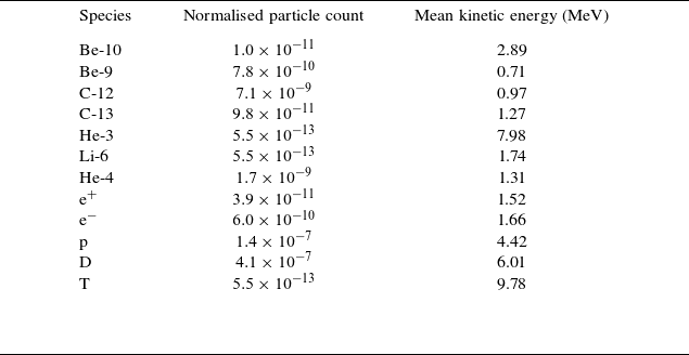
foil. The resulting charged particles are listed in table 1, where the dominant species consist of deuterons and protons (relative ratio
 $\sim 3:1$
). The number of ejected electrons is comparatively low and insufficient to neutralise the outgoing ion population. Charge separation effects and the resulting self-consistent electric fields are not captured in Geant4 and are instead modelled using PIC simulations in § 5.
Summary of charged particles emerging from the foil in Geant4. The particle count is normalised per source neutron per
 $\unicode{x03BC}$
m cm
 $^2$
(thickness–area) foil. The statistical uncertainty for deuteron and proton is
 ${\lesssim}0.1\,\%$
.

Table 1. Long description
The table presents data on charged particles produced from a foil in Geant4 simulations. It includes three columns: Species, Normalised particle count, and Mean kinetic energy (MeV). The table has 12 rows, each representing a different particle species. Row 1: Be-10, 1.0 x 10^-11, 2.89. Row 2: Be-9, 7.8 x 10^-10, 0.71. Row 3: C-12, 7.1 x 10^-9, 0.97. Row 4: C-13, 9.8 x 10^-11, 1.27. Row 5: He-3, 5.5 x 10^-13, 7.98. Row 6: Li-6, 5.5 x 10^-13, 1.74. Row 7: He-4, 1.7 x 10^-9, 1.31. Row 8: E+, 3.9 x 10^-11, 1.52. Row 9: E-, 6.0 x 10^-10, 1.66. Row 10: P, 1.4 x 10^-7, 4.42. Row 11: D, 4.1 x 10^-7, 6.01. Row 12: T, 5.5 x 10^-13, 9.78. The table shows the normalized particle count per source neutron per meter centimeter of foil thickness and area, along with the mean kinetic energy in mega electron volts for each species.
2.2. Sources of electrons
In addition to neutron–foil interactions, electrons can also be produced from material ablation at the foil. The optical image in figure 3(a) shows bright conical structures around the blast shield and foil holder, indicating possible ablation. Although the exact cause of this ablation is not yet understood, it is most likely driven by indirect processes such as scattered X-rays and/or stray laser light, which can bypass the blast shield in figure 1 and produce the foil heating seen in figure 3(b). Further comparison between measured yield by the MRS and neutron activation detectors (NAD) in figure 3(c) suggests an average material loss of
 ${\sim} 0.2 \, \mathrm{\unicode{x03BC} m}$
for each implosion experiment, which is confirmed by pre- and post-exposure foil thickness measurements at General Atomics. However, this high-density region is not expected to play a role in energy modulations (see Appendix A).
(a) Optical image showing bright conical structures around the MRS foil and blast shield. (b) Image of a partially burnt foil. (c) Ratio of the inferred yield from the MRS to the NAD for 36 shots fielded with the foil shown in (b).

Electrons can also be generated through X-ray photoionisation of residual gas in the target chamber. Multiple X-ray sources contribute to this process. Inside the hohlraum, soft X-rays follow a Planckian distribution with a radiation temperature
 $T_r \sim 300$
eV. In addition, M-band radiation (photon energies
 $\gt 1.8$
keV) is emitted from the laser beam interacting with high-Z coronal plasma wall blow-off (Lindl et al. Reference Lindl, Amendt, Berger, Glendinning, Glenzer, Haan, Kauffman, Landen and Suter2004; Dewald et al. Reference Dewald, Landen, Salmonson, Masse, Tabak, Smalyuk, Schiaffino, Heredia, Schneider and Nikroo2020). Harder X-rays are generated from bremsstrahlung in the hotspot (Khan et al. Reference Khan2018) and from hot electrons interacting with the capsule target (Hohenberger et al. Reference Hohenberger2013). In this context, the X-ray flux along the MRS line of sight (LOS) located at spherical angles
 $(\theta , \varphi ) = (73^{\circ }, 324^{\circ })$
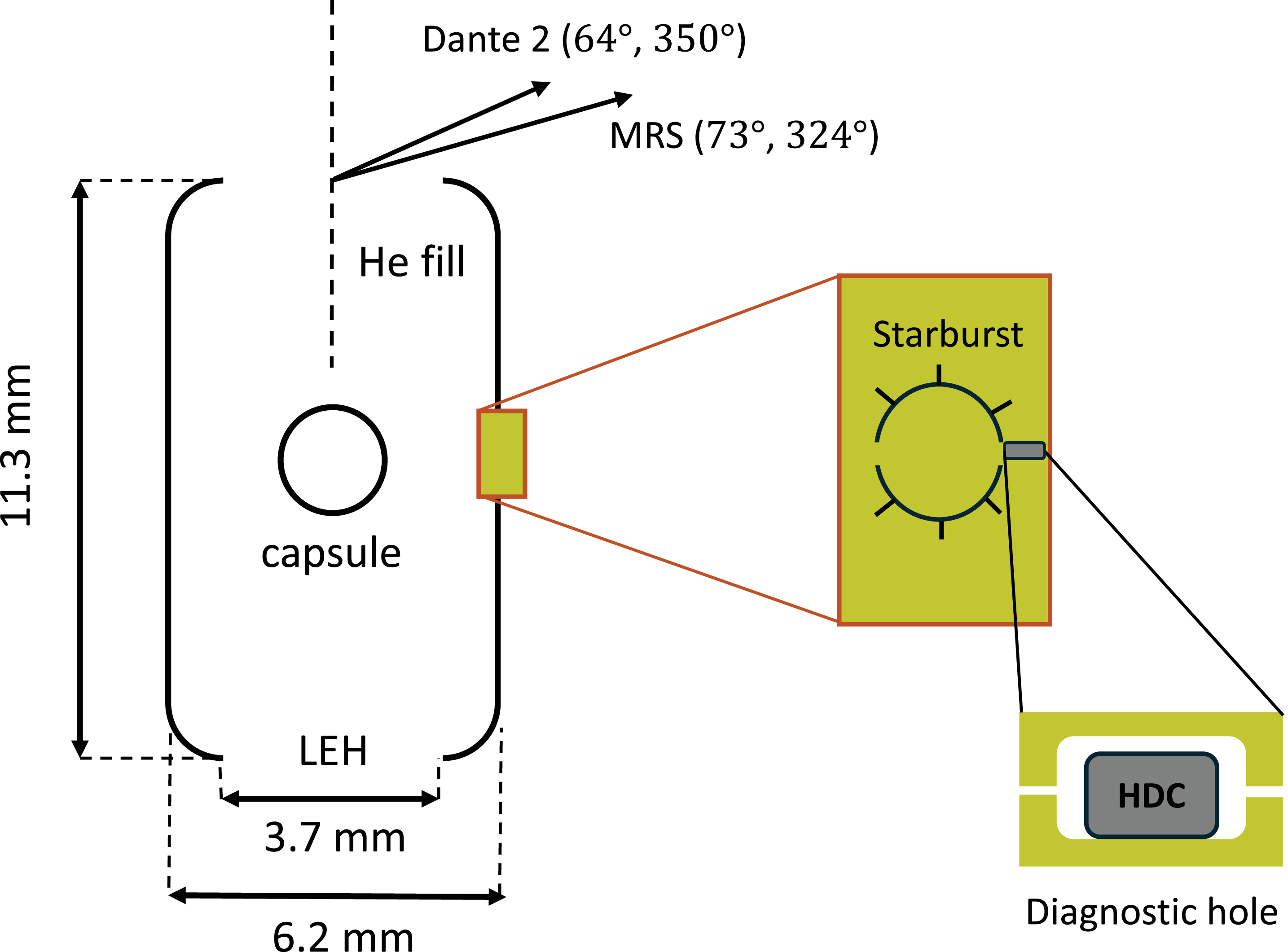
needs to be determined. X-rays could escape in this direction through the openings annotated in figure 4. One such feature is the starburst window, an empty circular cut-out used to image the DT ice layer on the inner surface of the capsule ablator. This opening provides a direct LOS from the capsule to the MRS. However, it is predicted to close within
 ${\sim} 1{-}2$
ns after the laser drive begins (Milovich et al. Reference Milovich, Dewald, Thomas, Robey and Landen2010). Therefore, the X-ray leakage through the starburst is limited.
Schematic of the nominal NIF hohlraum design. Possible sources of X-ray leakage in the MRS direction include the starburst window, DH and LEH. The DHs in other directions are not shown for clarity.

Another possible leakage path is through the diagnostic hole (DH) located slightly off-axis to the MRS at
 $(90^{\circ }, 315^{\circ })$
. HYDRA simulations (Marinak et al. Reference Marinak, Kerbel, Gentile, Jones, Munro, Pollaine, Dittrich and Haan2001) by Milovich et al. (Reference Milovich2020) show X-ray leakage through the DH at early times via small gaps and at later times by burning through the high-density-carbon (HDC) slab shown in figure 4. However, the DH contribution is expected to be minor since each DH subtends only
 ${\sim} 0.03$
sr from the TCC.
The last and most probable source of leakage is through the laser entrance holes (LEH). Although there is no direct LOS from the LEH to the MRS, the LEH effectively acts as a Lambertian source, emitting X-rays in all directions (Decker et al. Reference Decker1997; May et al. Reference May2015). The X-ray profile through the LEH is measured using Dante time-resolved X-ray spectrometers (Dewald et al. Reference Dewald2004). Data from Dante-2 are considered due to its angular proximity to the MRS at
 $(64^{\circ }, 350^{\circ })$
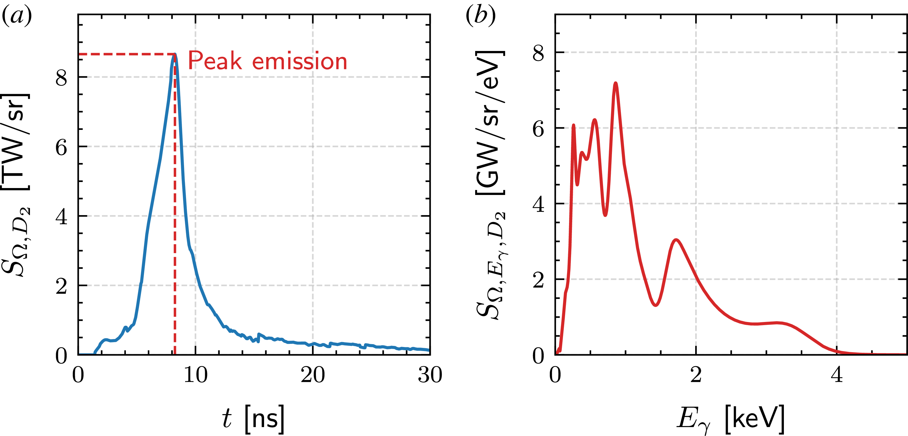
. The temporal profile of X-ray flux for experiment N240504-001 is shown in figure 5(a), where the total radiant energy per unit solid angle is
 $Q_{\varOmega , D_2} = \int S_{\varOmega , D_2} \, {\rm d}t \sim 37 \, \mathrm{kJ \, sr^{-1}}$
, where
 $S_{\varOmega , D_2}$
is the radiant intensity measured by Dante-2. Modelling the X-ray emission through the LEH as a Lambertian source (Decker et al. Reference Decker1997; May et al. Reference May2015), the total radiant energy per unit solid angle in the MRS direction is
 $Q_{\varOmega , \text{MRS}} = Q_{\varOmega , D_2} \cos (73^{\circ } ) / \cos (64^{\circ }) \sim 25 \, \mathrm{kJ \, sr^{-1}}$
. This calculation neglects attenuation effects and therefore serves as an upper-bound estimate. Figure 5(b) shows the X-ray energy spectrum at peak flux (
 $t\sim 8$
ns), which resembles the expected Planckian profile on top of the M-band signature seen at
 $E_\gamma \sim 2 \, \text{keV}$
.
(a) Temporal profile of X-ray flux measured by Dante-2 for experiment N240504-001. (b) Measured X-ray energy spectrum at peak flux at
 $t\sim 8$
ns.

Hard X-rays are typically measured using the FFLEX diagnostic along the equator (Hohenberger et al. Reference Hohenberger2013). Although FFLEX was not fielded on shot N240504-001, some simplified estimates can still be made to neglect the contribution of hard X-rays to photoionisation. Soft X-rays are typically
 ${\sim} 1$
keV, while hard X-rays are typically
 ${\gtrsim}10$
keV, resulting in an absorption factor
 ${\sim} 10^3$
higher for soft X-rays (Lemmon, Huber & McLinden Reference Lemmon2010). Moreover, the total energy of hard X-rays as measured by FFLEX is of the order of
 ${\sim} 10$
kJ (Rinderknecht Reference Rinderknecht2015), which is significantly less than the total energy of soft X-rays that escape through the LEH (
 ${\sim} 100$
kJ) (Chen et al. Reference Chen2025). For these reasons, soft X-rays emitted through the LEH are expected to be the dominant source of photoionisation.
2.3. Density and velocity distribution of photoelectrons
The density of photoelectrons is estimated using the X-ray absorption cross-section
 $\sigma _{\text{vac}}$
of air from the NIST database (Lemmon et al. Reference Lemmon2010). Following the approach of Swadling et al. (Reference Swadling2017), the X-ray attenuation due to residual gas along the MRS LOS is described by
 \begin{eqnarray} S_{\varOmega , \text{MRS}}(r) = \int S_{\varOmega ,\text{MRS}}(0) \exp (-\sigma _{\text{vac}}(E_\gamma ) n_{\text{vac}} r )\, {\rm d}E_\gamma , \end{eqnarray}
where
 $r$
is the radial distance from the TCC and
 $n_{\text{vac}}$
is the gas density inferred from the ambient pressure measured for each experiment (
 $p_{\text{vac}} = 1.22\times 10^{-5}$
torr for N240504-001). The initial (unattenuated) radiant intensity
 $S_{\varOmega , \text{MRS}}(0)$
seen by the MRS can be split into a product of the intensity and spectral component
 $S_{\varOmega ,\text{MRS}}(0) = I_{\varOmega , \text{MRS}}(0) f(E_\gamma )$
, where
 $f(E_\gamma )$
is the normalised photon spectrum approximated by the peak-flux profile in figure 5(b). This allows (2.2) to be rewritten as
 \begin{eqnarray} S_{\varOmega , \text{MRS}}(r) = I_{\varOmega , \text{MRS}}(0) \int f(E_\gamma ) \exp (-\sigma _{\text{vac}}(E_\gamma ) n_{\text{vac}} r ) \,{\rm d}E_\gamma , \end{eqnarray}
where
 $I_{\varOmega , \text{MRS}}(0)$
is pulled out of the integral. The energy density deposited into the residual gas along the MRS LOS is then computed as
 \begin{align} \frac {{\rm d}E}{{\rm d}V}(r)= \frac {{\rm d}\varOmega }{{\rm d}A} \int \frac {-{\rm d}S_{\varOmega , \text{MRS}}(r) } {{\rm d}r} \, {\rm d}t. \end{align}
Taking the X-ray energy spectrum as approximately constant in time leads to the following expression:
 \begin{eqnarray} \frac {{\rm d}E}{{\rm d}V}(r) = -\frac {Q_{\varOmega ,\text{MRS}}}{r^2} \frac {\rm d}{{\rm d}r} \int f(E_\gamma ) \exp (-\sigma _{\text{vac}}(E_\gamma ) n_{\text{vac}} r ) \, {\rm d}E_\gamma . \end{eqnarray}
Assuming all deposited energy in (2.5) is transferred to ionisation, the maximum average charge state is obtained by solving
 \begin{align} \frac {{\rm d}E}{{\rm d}V}(r)=n_{\text{vac}} \Bigg[(\bar {Z}-\lfloor \bar {Z}\rfloor ) I_{\lfloor \bar {Z}\rfloor -1}+\sum _{j=1}^{\lfloor \bar {Z}\rfloor } I_{j-1}\Bigg], \end{align}
where
 $I_j$
is the
 $j$
th ionisation energy per atom and
 $\lfloor \bar {Z}\rfloor$
is
 $\bar {Z}$
rounded down to an integer. Having found
 $\bar {Z}(r)$
, the electron density is found by
 $n_e (r) = \bar {Z}(r)n_{\text{vac}}$
.
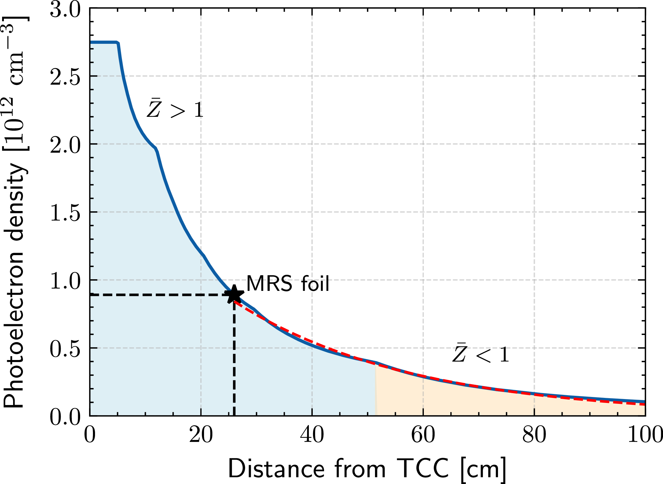
The numerical result of
 $n_e(r)$
is shown in figure 6, where the residual gas is assumed to be fully nitrogen for simplicity. Beyond the foil, the density of photoelectrons decays exponentially as given by
 $n_e(r\geqslant 26 \, \text{cm}) = n_{e,f} \exp ( -(r-26 \, \text{cm})/{L_n})$
, where
 $n_{e,f}\,\sim 9\times 10^{11} \,{\mathrm{cm}^{-3}}$
and
 $L_n \sim 32$
cm are extracted from the exponential fit in figure 6. These values serve as upper-bound estimates since they neglect attenuation and recombination effects.
Estimated density profile of photoionised electrons. The red region denotes
 $\bar {Z}\gt 1$
while the orange region denotes
 $\bar {Z} \lt 1$
. The foil and MRS aperture are located at
 $r=26$
cm and
 $r = 596$
cm, respectively. The initial flat profile indicates full ionisation of nitrogen (
 $\bar {Z}=7$
).

Given their low density, photoelectrons cannot effectively thermalise within the experimental time scale. Their angular distribution must therefore be considered. For unpolarised light, this is described by
 \begin{align} \frac {{\rm d}N_{e}}{{\rm d}\theta _{\gamma ,e}} \sim \sin \theta _{\gamma ,e} - \frac {\beta (E_\gamma ) \sin \theta _{\gamma ,e}}{2}P_2(\cos \theta _{\gamma ,e}), \end{align}
where
 $\theta _{\gamma ,e} \in [0^\circ , 180^\circ ]$
is the angle between the photon and electron velocity,
 $\beta$
is the asymmetry parameter and
 $P_2$
is the second-order Legendre polynomial (Yeh & Lindau Reference Yeh and Lindau1993; Reid Reference Reid2003). Since the X-ray energies are well above the ionisation threshold (
 ${\sim} 10$
eV), the electrons follow the X-ray energy distribution weighted by the absorption cross-section
 ${\rm d}N_e/{\rm d}E_e \sim f(E_\gamma ) \sigma _{\text{vac}}(E_\gamma )$
. The electron velocity distribution function (EVDF) can be obtained by first sampling the energy from
 ${\rm d}N_e/{\rm d}E_e$
and then sampling the angle from (2.7). The resultant EVDF is displayed in figure 7, where
 $v_{r}$
and
 $v_{\perp }$
correspond to the radial and transverse components, respectively, in the spherical coordinate system of the target chamber. When the neutrons arrive at the foil, this EVDF is expected to have deviated from its initial profile due to electron–electron interactions, as will be discussed in §§ 3 and 4.
(a) Two-dimensional velocity distribution function of photoionised electrons, obtained by sampling their angular and energy distribution. Here,
 $v_{r}$
and
 $v_{\perp }$
correspond to the radial and transverse components in the spherical coordinate system of the target chamber, respectively. (b) One-dimensional velocity distribution in terms of
 $v_r$
. (c) One-dimensional velocity distribution in terms of
 $v_\perp$
.

Figure 7. Long description
Panel A: A two-dimensional heatmap showing the velocity distribution function of photoionised electrons. The horizontal axis represents the radial velocity component (v_r) in units of 10^9 cm/s, ranging from -2 to 2. The vertical axis represents the transverse velocity component (v_t) in units of 10^9 cm/s, also ranging from -2 to 2. The heatmap displays a circular pattern with higher intensity around the center, indicating the concentration of electron velocities. Panel B: A line graph showing the one-dimensional velocity distribution in terms of the radial velocity component (v_r). The horizontal axis represents the radial velocity component (v_r) in units of 10^9 cm/s, ranging from 0 to 2. The vertical axis represents the distribution function, ranging from 0 to 0.5. The line graph shows a peak around 1, indicating the most probable radial velocity. Panel C: A line graph showing the one-dimensional velocity distribution in terms of the transverse velocity component (v_t). The horizontal axis represents the transverse velocity component (v_t) in units of 10^9 cm/s, ranging from 0 to 0.5. The vertical axis represents the distribution function, ranging from 0 to 2. The line graph shows a peak around 0.2, indicating the most probable transverse velocity.
2.4. Effect of the blast shield
It is important to understand how the MRS blast shield factors into our previous estimates. The shield is made from a tantalum plate (
 $Z = 73$
, radius
 $\sim$
2 cm, thickness
 $\sim$
1.57 mm) designed to block all debris and X-rays from the implosion. This creates a ‘shadow region’ behind the shield where photoionisation is suppressed. However, ionisation can still occur in adjacent regions around the shield. Based on the bulk transverse velocity in figure 7(c), photoelectrons can travel a distance of 2 cm in
 ${\sim}$
2 ns, giving them ample time to populate the shadow region before 14.1 MeV neutrons arrive at the foil (
 ${\sim}5$
ns after the X-rays arrival at the foil).
3. Analysis of beam–plasma instabilities
3.1. Deuteron–electron modes
To explore the possible ion–electron modes, a simplified model of deuterons streaming through a uniform plasma is considered. The deuterons are modelled as a beam with
 $\langle E_d \rangle \sim 12.5$
MeV, while the electrons follow the EVDF shown in figure 7(b). Collisional effects can be safely ignored due to the low electron density (
 $n_e \sim 10^{11} \,{\mathrm{cm}^{-3}}$
). Under these conditions, electrostatic or weakly electromagnetic instabilities are expected to occur (Mima et al. Reference Mima, Fuchs, Taguchi, Alvarez, Marquès, Chen, Tajima and Perlado2018).
The electromagnetic beam-Weibel instability has a maximum growth rate of
 $\omega _b v_b/c$
, where
 $\omega _b = (n_de^2/m_d\epsilon _0)^{1/2}$
is the deuteron plasma frequency,
 $n_d$
is the initial deuteron density,
 $e$
is the elementary charge,
 $m_d$
is the deuteron mass,
 $\epsilon _0$
is the permittivity of free space and
 $v_b$
is the beam velocity (Takabe Reference Takabe2023). Based on the reported yield, burn width and foil set-up,
 $n_d \sim 10^{10} \,{\mathrm{cm}^{-3}}$
near the foil rearside, which gives an e-folding time of
 ${\sim}70$
ns. Due to angular divergence of deuterons, the beam density drops significantly within this time scale, which renders this instability negligible.
The electrostatic TSI occurs when the beam velocity
 $(v_b \sim 3.4 \times 10^9 \,{\mathrm{cm}\, \mathrm{s}^{-1}})$
exceeds the electron velocity spread (Chen Reference Chen2012), a condition satisfied according to the EVDF illustrated in figure 7(b). The TSI is evaluated by considering the following dispersion relation:
 \begin{align} D(\omega ,k) = 1 + \sum _j \frac {\omega ^2_{p,j}}{k_r} \int \frac {\partial \hat {f}_j (v_r) / \partial v_r}{\omega - k_rv_{r,j}}\, {\rm d}v_r = 0, \end{align}
where
 $\hat {f}(v_r)$
is the normalised velocity distribution function,
 $k_r$
is the radial wavevector component and
 $\omega _{p,j} = (n_j Z_j^2 e^2 / m_j \epsilon _0)^{1/2}$
is the plasma frequency (Chen Reference Chen2012). Here,
 $n_j$
is the density and
 $Z_j$
is the charge state of species
 $j\in \{\text{electron, ion (nitrogen), deuteron} \}$
. For cold species, their velocity distributions are approximated as Dirac deltas centred at the drift velocity
 $\hat {f}_j(v_r) = \delta (v_r - v_{d,j})$
. Applying this to (3.1) and integrating by parts gives
 \begin{align} 1 - \frac {\omega _{\text{pe}}^2}{\omega ^2} - \frac {\omega _{\text{pi}}^2}{\omega ^2} - \frac {\omega _b^2}{(\omega - k_r v_b)^2} = 0, \end{align}
where
 $\omega _{\text{pe}}$
and
 $\omega _{\text{pi}}$
are the electron and ion plasma frequencies of the ambient plasma. Since
 $\omega _{\text{pi}} \ll \omega _{\text{pe}}$
, (3.2) reduces to
 \begin{align} \big(\omega ^2 - \omega _{\text{pe}}^2\big)(\omega - k_r v_b)^2 = \omega _b^2 \omega ^2. \end{align}
In the perturbative regime of
 $\alpha = n_b/n_e \ll 1$
, the unstable mode occurs at
 $\omega \sim k_r v_b$
. Assuming
 $\omega = k_rv_b + i\gamma$
, the maximum TSI growth rate is
 \begin{align} \gamma _{\text{TSI}} = \frac {\sqrt {3} \, \omega _{\text{pe}}}{2} \left ( \frac {m_e n_d}{2 m_d n_e} \right )^{1/3}, \end{align}
which corresponds to an e-folding time of
 ${\sim}3$
ns. Given that it takes
 ${\sim}$
200 ns for aperture-selected deuterons to reach the MRS, there is more than enough time for TSI to develop. As the deuterons propagate, a radial electric wake field
 $\mathcal{E}_r$
is excited. For a radially thin beam with no transverse variation (Hu et al. Reference Hu, Song, Zhao and Wang2013),
 $\mathcal{E}_r$
is evaluated as
 \begin{align} \mathcal{E}_r(r,t) = -\frac {e n_d}{\epsilon _0 k_p} \sin \!\big (k_p (r - v_b t)\big ) \mathcal{H}(r - v_b t), \end{align}
where
 $r - v_bt$
is the radial position in the beam’s frame and
 $k_p=\omega _{\text{pe}}/v_b$
is the excited wavenumber. The Heaviside step function
 $\mathcal{H}(r-v_b t)$
imposes that the wake field only forms behind the beam. This oscillatory field modulates deuteron energies through alternating regions of acceleration and deceleration. While the analytical approach provides a qualitative understanding, PIC simulations are required to self-consistently model the nonlinear evolution of energy modulations.
3.2. Electron–electron modes
The bimodal EVDF represents two counter-streaming electron populations, which can drive the electron Weibel instability (EWI). The resulting magnetic field may deflect deuterons and therefore warrants further investigation. Adopting the analytical treatment of Davidson et al. (Reference Davidson, Hammer, Haber and Wagner1972), the bimodal EVDF shown in figure 7(a) is approximated by
 \begin{align} f_{0,e}(v_r, v_\perp ) \sim \exp \!\left [-\!\left (\frac {v_r}{\Delta v_r}\right )^{\!2}\right ] \left [\exp \!\left (-\!\left (\frac {v_\perp - v_{d,e}}{\Delta v_\perp }\right )^{\!2}\right ) + \exp \!\left (-\!\left (\frac {v_\perp + v_{d,e}}{\Delta v_\perp }\right )^{\!2}\right )\right ], \end{align}
where
 $\Delta v_i = (2k_B T_i /m_e)^{1/2}$
is the velocity spread in direction
 $i\in [r, \perp ]$
,
 $k_B$
is the Boltzmann constant and
 $v_{d,e}$
is the electron drift velocity in the transverse direction. The parameters
 $T_r \sim 290 \, \text{eV}$
and
 $T_\perp \sim 57 \, \text{eV}$
are obtained from fitting the distributions in figure 7(b,c), which characterise the directional velocity spread and do not imply thermal equilibrium.
In this case, the dispersion relation for the EWI (Davidson et al. Reference Davidson, Hammer, Haber and Wagner1972) is expressed by
 \begin{align} c^{2} k^{2} - \varOmega _{k}^{2} + \omega _{pe}^{2} \left [ 1 - \frac {k_B T_{\perp } + m_e V_{0, \perp }^{2}}{k_B T_{\parallel }} \right ] - \omega _{pe}^{2} \left [ \frac {k_BT_{\perp } + m_e V_{0, \perp }^{2}}{k_B T_{\parallel }} \right ] \xi _e Z(\xi _e) = 0, \end{align}
where the ion’s motion is neglected (
 $\omega _{\text{pi}}^2 \ll \omega _{\text{pe}}^2$
) and
 \begin{align} Z\left (\xi _e\right ) \equiv \pi ^{-1 / 2} \int _{-\infty }^{\infty } {\rm d} x \frac {\exp (-x^2)}{x-\xi _e}, \quad \xi _e \equiv \frac {\omega _k+i \gamma _k}{k\left (2 k_B T_{r} / m_j\right )^{1 / 2}}, \quad \varOmega _k = \omega _k + i\gamma _k. \end{align}
Analysis of (3.7) depends on the anisotropy
 $A = (k_BT_\perp + mv_{d,e}^2 - k_BT_r) /k_B T_r$
, where the term
 $k_BT_\perp + mv_{d,e}^2$
captures the effective velocity spread in the transverse direction (Davidson et al. Reference Davidson, Hammer, Haber and Wagner1972). A simple analytic solution exists in the limits of
 $A \ll 1$
or
 $A \gg 1$
(Davidson et al. Reference Davidson, Hammer, Haber and Wagner1972). In this case, however,
 $A \sim 3.6$
, placing it in an intermediate regime that requires numerical evaluation of the dispersion relation. Iteratively solving (3.7) yields a fastest EWI growth time of
 ${\sim}3\,\mathrm{ns}$
, allowing sufficient time for the instability to develop. The corresponding magnetic field strength and its effect on deuteron trajectories cannot be determined analytically and are instead examined using a two-dimensional PIC simulation in § 4.
In addition to the EWI, oppositely streaming electrons can also drive the electron–electron TSI mode. The corresponding e-folding time of
 ${\sim} 80 \, \text{ps}$
suggests that TSI can develop and saturate well before neutrons reach the foil. As kinetic energy is transferred into electrostatic waves, the initial bimodal EVDF described in (3.6) is expected to flatten (Hou et al. Reference Hou, Chen, Yu and Wu2015). This effect can be estimated using a simplified two-dimensional PIC simulation, as is discussed in § 4.
4. Pre-neutron arrival simulation
Prior to the neutron arrival at the foil, photoionised electrons can interact through the EWI and TSI. This effect is simulated in two dimensions using the PIC code epoch (Arber et al. Reference Arber2015; Bennett et al. Reference Bennett, Brady, Schmitz, Ridgers, Arber, Evans and Bell2017) which models the electron–electron interactions up to when neutrons arrive at the foil. The photoionised electrons are initialised with a uniform density
 $n_{e} = 10^{11} \,{\mathrm{cm}^{-3}}$
and velocities
 $(v_r, v_\perp )$
externally sampled from the bimodal profile in figure 7(a). The simulation domain spans
 ${\sim} 10$
cm in each direction with a cell size
 $\varDelta _r =\varDelta _\perp = 0.5 \lambda _D$
, where
 $\lambda _D = ( \epsilon _0 k_B T_e / m_e e^2)^{1/2}$
is the Debye length. Here,
 $\lambda _D$
is calculated with
 $T_e\,=\,\text{min}(T_r, T_\perp )$
to ensure a sufficient spatial resolution. Periodic boundary conditions are used. Each cell contains 128 fifth-order macroparticles, which helps suppress numerical heating and accurately resolve unstable modes (McMillan Reference McMillan2020).
Figure 8(a) shows the temporal evolution of the out-of-plane magnetic field
 $B_z(r,y)$
, where characteristic filamentation of the EWI is observed (Takabe Reference Takabe2023). The final magnetic field strength is
 ${\sim} 0.4$
mT. Even in the upper limit of a uniform field, 12.5 MeV deuterons are deflected by
 ${\sim} 0.2^\circ$
. This only reduces the forward kinetic energy by 100 eV, which is negligible compared with the MRS energy resolution (full width at half-maximum (FWHM)
 $\sim$
200 keV) (Gatu Johnson et al. Reference Gatu Johnson2022). Therefore, the magnetic field generated by the EWI cannot meaningfully deflect deuterons.
Figure 8(b) depicts the temporal evolution of the magnetic field energy. The initial e-folding time is found to be
 ${\sim} 0.50\pm 0.05$
ns, which is faster than expected (
 ${\sim} 3$
ns). This is likely because the Gaussian approximations of (3.6) do not account for the correlations between
 $v_r$
and
 $v_\perp$
, which result in an underestimated anisotropy and growth rate. This explanation is supported by Appendix B, which shows a reasonable agreement between PIC simulation and theory when using the idealised bi-Maxwellian distribution.
(a) Temporal evolution of the magnetic field profile
 $B_z(r,y)$
obtained from PIC. At
 $t=0$
(not shown),
 $B_z(r,y)=0$
. The development of filaments as the magnetic field grows is characteristic of the EWI. The simulation box size is
 ${\sim} 10 \,\mathrm{cm}\times 10 \,\mathrm{cm}$
. (b) Temporal evolution of the magnetic field energy obtained from PIC simulation (black). An exponential fit (red) is applied to the linear regime, giving an e-folding time of
 $0.50 \pm 0.05 \, \mathrm{ns}$
.

The initial and final velocity distributions of electrons as determined from the two-dimensional PIC simulation are shown in figure 9. As expected from TSI interactions, the initial bimodal structure in
 $v_y$
becomes merged and flattened (Hou et al. Reference Hou, Chen, Yu and Wu2015). The final distribution in figure 9(b) then serves as input for the post-neutron arrival (at the foil) simulations.
(a) Initial electron velocity distribution (bimodal). (b) Final electron velocity distribution (flattened).

5. Post-neutron arrival simulation
5.1. Simulation set-up
The post-neutron arrival simulations model the transport of deuterons through a tenuous plasma from the foil backside to the MRS magnet aperture (see figure 10). The initial domain spans
 $r \in [26, 150]$
cm and
 $y \in [-1, 1]$
cm with a uniform grid size
 $\varDelta _r = \varDelta _\perp = 0.7\lambda _D$
. A moving window is applied to ensure aperture-selected deuterons can reach
 $r = 596$
cm, where a particle probe representative of the MRS records their kinetic energies for direct comparison with the experiment.
(a) Diagram of the two-dimensional PIC simulation frame relative to the spherical target chamber geometry (not to scale). The blue line indicates the MRS LOS. (b) External sampling routine of recoil particles. The neutron energy is sampled based on the reported
 $(Y_n, \rho R, T_i)$
, accounting for Doppler broadening. Its birth time is drawn from a Gaussian burn duration with a FWHM of
 $\tau _{\text{BW}}$
. A recoil particle is generated once the neutron hits the foil. These steps are repeated until sufficient sampling is reached.

The ambient electrons are initialised with 150 fifth-order macroparticles per cell based on the density profile shown in figure 6 and modified EVDF described in § 4. Due to uncertainties in the X-ray flux, the terms
 $n_{e,f}$
and
 $L_n$
are treated as free parameters. The recoil protons and deuterons are each initialised with
 $2\times 10^8$
macroparticles, which is sufficient for numerical convergence. Their weight is determined from the particle numbers in table 1, scaled according to the reported neutron yield and foil configuration of experiment N240504-001. Due to the complex initial phase-space distributions, the recoil particles are externally sampled and loaded into the simulation via binary files, as shown in figure 10(b). The built-in particle injector in epoch is avoided to prevent the formation of a large sheath electric field, which could distort the initial deuteron energy spectrum.
5.2. Simulation results
5.2.1. Experiment N240504-001
A parameter scan indicates that
 $n_{e,f}\sim (2.5\pm 0.5)\times 10^{11} \,{\mathrm{cm}^{-3}}$
and
 $L_n \sim 17\pm 3$
cm provide a reasonable match to the modulation wavelength in the experiment (simulation: 610 keV; experiment: 590 keV). Compared with the analytical estimates in § 2, these values are lower by a factor of 3–5, though still within the same order of magnitude. This discrepancy likely arises from X-ray attenuation by thermomechanical structures within the LEH assembly, which is not included in the model (Swadling et al. Reference Swadling2025). The resulting spectrum is shown in figure 11(a); the remaining differences between simulation and experiment may reflect missing details in the assumed EVDF.
(a) Comparison between the simulated (blue) and experimental (orange) deuteron energy spectra. The dashed black line shows the assumed initial spectrum. Note that the error bars are smaller than the plot markers. (b) Normalised modulation profile of the simulated spectrum calculated from (5.1).

The energy modulation is directly quantified in figure 11(b). Given the initial spectrum
 $f_0$
and modulated spectrum
 $f_1$
, the normalised modulation profile is defined as
 \begin{align} \mathcal{M}(E_d) = \frac {f_1(E_d) - f_0(E_d)}{f_0(E_d)}. \end{align}
The simulated
 $\mathcal{M}(E_d)$
profile in figure 11(b) shows an approximately uniform modulation wavelength
 $\lambda _m \sim 600 \, \text{keV}$
and modulation amplitude
 $\mathcal{A}_m \sim 0.1$
. To understand these results, the beam–plasma instability analyses in § 3 are revisited. By comparing the ratio of the magnetic energy to electric energy at various times,
 \begin{eqnarray} \frac {\int |B|^2 \ {\rm d}V}{\int \mu _0\epsilon _0 |\mathcal{E}|^2 \ {\rm d}V} \lesssim 10^{-2}, \end{eqnarray}
it is deduced that the contribution from the beam-Weibel instability is relatively minor. Figure 12 shows spatially oscillatory structures in
 $\mathcal{E}_r$
at various times, which is indicative of the electrostatic TSI. The observed spatial wavelength at
 $t=2$
ns, for example, is
 ${\sim} 0.8$
cm, consistent with the analytical prediction
 $\lambda _{\text{TSI}} = 2\pi v_b / \omega _{\text{pe}}$
evaluated at the local plasma frequency. In addition, the induced electric field is of order kV cm−1 in magnitude, as predicted by (3.5). The induced electric field diminishes over time due to the angular divergence of the deuterons.
Top row: energy phase space of aperture-selected deuterons at different times. The radial directed electric field, averaged over
 $y$
, is overlaid in magenta. Bottom row: corresponding radial profiles of the aperture-selected deuteron number density at the same times. The radial axis values vary due to the applied moving window.

(a) Aperture-selected deuteron energy spectra at selected times. Modulations mostly occur in the early times when the induced electric field is stronger. Saturation is observed at around
 $t \sim 60$
ns. (b) Modulation amplitude averaged between 8 and 12 MeV as a function of the local density ratio at
 $t = 0$
. The vertical error bars represent the standard deviation of each data point.

Figure 13. Long description
Panel A: A line graph shows deuteron energy spectra at various times. The x-axis represents deuteron energy in MeV, ranging from 8 to 13 MeV. The y-axis represents deuteron count per MeV, ranging from 0 to 5. Multiple lines, each representing a different time point from 0 to 160 nanoseconds, show the energy spectra. The lines exhibit modulations, particularly in the early times, with saturation observed around 100 nanoseconds. Panel B: Another line graph shows the modulation amplitude averaged between 8 and 12 MeV as a function of the local density ratio at t=0. The x-axis represents the local density ratio, ranging from 1.0 to 2.5 times 10^-1. The y-axis represents the modulation amplitude in units of 10^-1 MeV, ranging from 0 to 1.0. Data points with vertical error bars indicate the standard deviation of each data point, showing an increasing trend in modulation amplitude with increasing local density ratio.
To make the connection between spatial and energy modulations, we analyse the energy phase-space diagram in figure 12, where the excited
 $\mathcal{E}_r$
averaged along the y axis is overlaid in magenta. At a given time
 $t=t_1$
, deuteron energy relates to the radial position through
 $E_d(r, t_1) = a(t_1) r + b(t_1)$
, where
 $a(t_1)$
and
 $b(t_1)$
parametrise the straight line in the energy phase-space diagram. In the simulation, the wavelength of energy modulation stabilises by
 $t \sim 2$
ns (see figure 13
a), justifying the constant
 $a(t_1 = 2 \, \text{ns})$
for our purposes. Assuming this behaviour is similar across different
 $(n_d, n_e)$
, it is expected that
 $\lambda _m \sim a(t_1 = 2 \, \text{ns}) \lambda _{\text{TSI}}$
, which scales with
 $n_e^{-1/2}$
. The other modulation quantity of interest is the amplitude
 $\mathcal{A}_m$
, which is expected to scale with the amplitude of the electrostatic potential
 $\varPhi (r, t)$
based on dimensional considerations. Integrating (3.5) leads to
 \begin{align} \varPhi (r, t) &= \frac {e n_d}{\varepsilon _0 k_p^2} \cos [k_p (r - v_b t)] \mathcal{H}(r - v_b t) \nonumber \\ & = \frac {n_d}{n_e} \frac {m_e v_b^2}{e} \cos [k_p (r - v_b t)] \mathcal{H}(r - v_b t), \end{align}
which scales proportionally with the density ratio
 $\alpha = n_d/n_e$
. To validate these scaling relations and gain a broader understanding of modulations,
 $(n_d, n_e)$
are systematically varied based on the realistic yield, laser energy and vacuum pressure. Each case is evolved to the same end time as shot N240504 to enable a consistent comparison of the resulting energy modulations.
To characterise the modulation amplitude,
 $\langle \mathcal{A}_m \rangle$
is defined as the average peak height within the range
 $E_d \in [8,12]$
MeV, where the amplitude remains approximately uniform. As shown in figure 13(b),
 $\langle \mathcal{A}_m \rangle$
increases linearly with the initial local density ratio
 $\alpha (t=0)$
, consistent with the scaling from (5.3). This implies that when
 $\alpha$
is small – due to either low deuteron density (e.g. low-yield experiments) or high electron density (e.g. high vacuum pressure or high X-ray leakage) – the resulting modulation is correspondingly weak and may not be seen in experiments. The modulation
 $\lambda _m$
is observed to decrease as
 $n_e$
increases. Within the realistic
 $n_e$
range,
 $\lambda _m$
varies between 500 and 700 keV. However, the difference is small and not always detectable within the energy bin width of 50 keV. There are two important caveats about these results. First, this scaling is valid only in the perturbative regime. For
 $\alpha \gtrsim 1$
, the electric field evolution can become highly nonlinear due to the formation of forerunner electrons (Hara, Kaganovich & Startsev Reference Hara, Kaganovich and Startsev2018), which can significantly alter the deuteron energy spectrum. This effect arises in the nonlinear phase of TSI when a fraction of the initially trapped electrons becomes de-trapped and accelerates ahead of the deuteron beam, which drives a secondary TSI with the background electron population. Second, sufficient ionisation is required to sustain a plasma. At very low electron densities, TSI is expected to vanish, and interactions with neutrals are expected to dominate.
6. Sensitivity study
A synthetic data study was conducted to assess the impact of modulations on high-yield experiments. The synthetic neutron spectrum is initialised by parameters
 $(Y_n$
,
 $T_i$
,
 $\rho R)$
. The primary component is modelled as a Gaussian distribution with its mean and width determined by the ion temperature
 $T_i$
, while the down-scatter component scales linearly with
 $\rho R$
(Ballabio, Källne & Gorini Reference Ballabio, Källne and Gorini1998). The model neutron spectrum is then convolved with the MRS response function to give the measured deuteron spectrum
 $f_0(E_d)$
. To mock-up energy modulations in the deuteron spectrum, a sinusoidal profile with uniform amplitude and wavelength is used:
 \begin{align} \mathcal{M} (E_d)= 1 + \mathcal{A}_m \sin \left (\frac {2\pi }{\lambda _{\text{m}}} (E_d + \delta E) \right ), \end{align}
where
 $\delta E \in [-50,50]$
keV is a random energy shift. The resultant modulated spectrum is expressed as
 \begin{align} f_{\text{1}}(E_d) = f_0(E_d)\mathcal{M}(E_d) \frac {N_d}{N_{{m}}}, \end{align}
where the term
 $N_d/N_{{m}}$
redistributes the deuterons to conserve the total count.
Afterwards, Poisson-distributed noise and realistic background subtraction are applied to each energy bin of
 $f_1(E_d)$
. The background accounts for intrinsic plastic defects and neutron-induced tracks in CR-39 analysis, which can affect the measured deuteron spectrum in the down-scattered region (Casey et al. Reference Casey2011). With the modulated deuteron spectrum generated,
 $Y_n$
,
 $T_i$
and
 $\rho R$
are determined from the optimal fit parameters. Our fitting routine employs the curve_fit function from the SciPy library (Virtanen et al. Reference Virtanen2020), where more weight is given to the data points with lower uncertainties. The statistical uncertainty in each energy bin is estimated based on the deuteron count and background contribution.
Analytical theory and simulation results suggest the main levers of energy modulations are the deuteron density
 $n_d$
and background electron density
 $n_e$
. The deuteron density scales as
 \begin{align} n_d = \frac {N_d}{V_d} \propto \frac {Y_n d_{\kern-1pt f} A_{\kern-1.2pt f}}{\tau _{\text{BW}}} ,\end{align}
where
 $V_d$
is the initial volume occupied by deuterons,
 $d_{\kern-1pt f}$
is the foil thickness,
 $A_{\kern-1.3pt f}$
is the foil area and
 $\tau _{\text{BW}}$
is the burn width.
Since photoelectrons are produced by soft X-rays ionising the residual gas in the target chamber,
 $n_e$
is expected to scale with the laser drive energy and residual gas pressure:
 $n_e \propto E_L^{0.6} p_{\text{vac}}$
(see Appendix C for
 $E_L$
scaling). Combining this with (6.3) yields the scaling for
 $\mathcal{A}_m$
:
 \begin{align} \mathcal{A}_m \sim \frac {n_d}{n_e} \propto \frac {Y_n d_{\kern-1pt f} A_{\kern-1.2pt f}}{E_L^{0.6} p_{\text{vac}} \tau _{\text{BW}}}, \end{align}
where the modulation amplitude
 $\mathcal{A}_m$
correlates with yield. In contrast, the modulation wavelength
 $\lambda _m$
is less restricted and therefore allowed to vary between 500 and 700 keV. To simplify the analysis of the synthetic study, the burn width
 $\tau _{\text{BW}}$
and vacuum pressure
 $p_{\text{vac}}$
are assumed as fixed. This leaves
 $(Y_n, d_{\kern-1pt f}, A_{\kern-1.3pt f}, E_L)$
as the driving factors for modulations. For the scaling in (6.4), shot N240504-001 is used as the reference point.
A typical high-yield implosion could have the following parameters:
 $Y_n \sim 10^{17}$
,
 $T_i \sim 10$
keV,
 $\rho R \sim 500 \, \mathrm{mg\,cm^{-2}}$
and
 $E_L \sim 2$
MJ. The foil configurations
 $(d_{\kern-1pt f}, A_{\kern-1.3pt f})$
in these experiments include
 $(52.3\,\mathrm{\unicode{x03BC} m}, 3 \,{\mathrm{cm}^2})$
and
 $(56.7\,\mathrm{\unicode{x03BC} m}, 0.5 \,{\mathrm{cm}^2})$
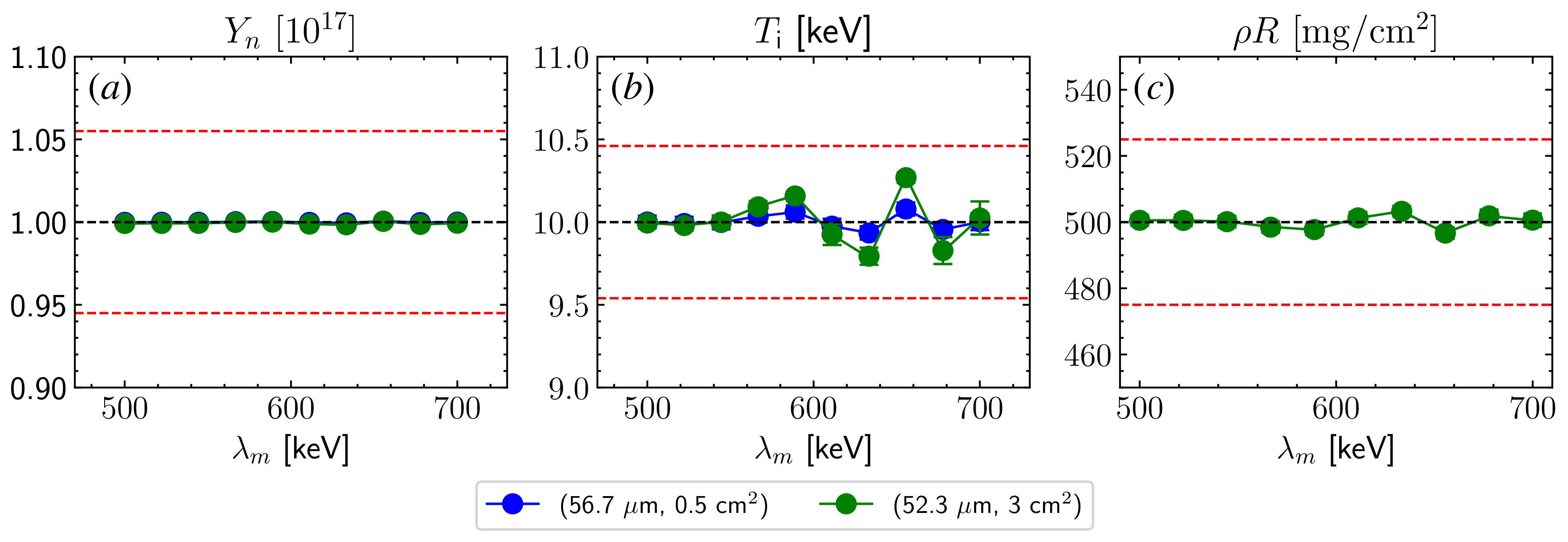
. Figure 14 shows the effect of energy modulations on the MRS-inferred parameters averaged over 1000 synthetic spectra. For both foil configurations, the results are are within the expected systematic uncertainties:
 $\Delta Y_n/Y_n \leqslant 5.5\,\%$
,
 $\Delta \rho R/ \rho R \sim 5\,\%$
and
 $\Delta T_i\sim 0.46$
keV. Therefore, the impact of modulations remains negligible at
 $Y_n \sim 10^{17}$
, which also explains why they have only recently become apparent in the data.
Effect of energy modulations on the inferred (a) neutron yield, (b) ion temperature and (c) areal density. The error bars show the standard deviation over 1000 synthetic spectra and are sometimes smaller that the marker size. The dashed red lines mark the acceptable uncertainty ranges:
 $\Delta Y_n/Y_n \leqslant 5.5\,\%$
,
 $\Delta \rho R/ \rho R \sim 5\,\%$
and
 $\Delta T_i\sim 0.46$
keV. Here,
 $Y_n \sim 10^{17}$
,
 $\rho R \sim 500 \, \mathrm{mg\,cm^{-2}}$
,
 $T_i \sim 10$
keV and
 $E_L \sim 2$
MJ. Note that in practice the
 $(56.7\,\mathrm{\unicode{x03BC} m}, 0.5 \,{\mathrm{cm}^2})$
foil configuration is not used to infer
 $\rho R$
.

Modulations have also been observed in experiments with
 $Y_n\sim 10^{18}$
,
 $T_i \sim 15$
keV and foil configuration
 $(56.7\,\mathrm{\unicode{x03BC} m},\ 0.5\,{\mathrm{cm}^2})$
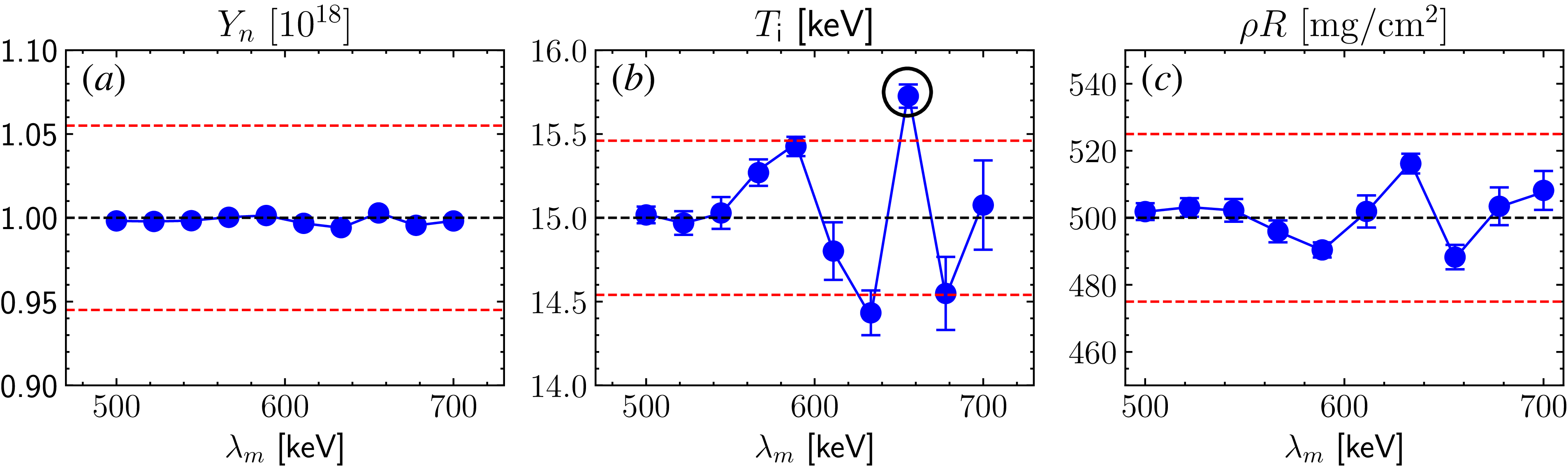
. Repeating the previous analysis for this scenario leads to figure 15, where the errors introduced by energy modulations remain largely acceptable, except for the one circled in black. As
 $Y_n$
increases further, the impact of modulations will eventually become non-negligible. Here, the potential approaches to mitigate this effect are discussed.
One proposed solution is to move the foil back by an additional
 ${\sim} 50$
cm, which would reduce the neutron flux by a factor of
 ${\sim} 10$
and similarly lower
 $n_d$
. While this would decrease the amplitude of modulations, it would not eliminate them entirely. Photoionised electrons can still populate the shadowed region before neutrons reach the foil, allowing modulations to persist. A more permanent solution as proposed by Wink et al. (Reference Wink2024) is to position the foil close to the MRS aperture. In this case, photoionised electrons would not have an opportunity to interact with deuterons, preventing the onset of TSI and consequently energy modulations.
Effect of energy modulations on the inferred (a) neutron yield, (b) ion temperature and (c) areal density of the
 $(56.7\,\mathrm{\unicode{x03BC} m}, 0.5 \,{\mathrm{cm}^2})$
foil configuration. The black circle indicates the data point outside the acceptable range. The set-up is the same as for figure 14 except
 $Y_n \sim 10^{18}$
and
 $T_i \sim 15$
keV.

Figure 15. Long description
Three line graphs depict the effect of energy modulations on neutron yield, ion temperature, and areal density. Panel A: The line graph shows neutron yield (Yn) in units of 10^18 on the vertical axis and energy modulation (λm) in keV on the horizontal axis. The data points are relatively stable around the value of 1.00 with minor fluctuations. Panel B: The line graph shows ion temperature (Ti) in keV on the vertical axis and energy modulation (λm) in keV on the horizontal axis. The data points fluctuate more significantly, with a notable peak around 650 keV, which is circled and indicated as outside the acceptable range. Panel C: The line graph shows areal density (ρR) in mg/cm^2 on the vertical axis and energy modulation (λm) in keV on the horizontal axis. The data points show minor fluctuations around the value of 500.
7. Conclusion
To summarise, this work indicates that energy modulations observed in the MRS data obtained at the NIF are driven by the TSI between deuterons and ambient electrons. The modulation features obtained in shot N240504-001 are reasonably reproduced by PIC simulations. A realistic density scan reveals that modulation amplitude scales linearly with the deuteron-to-electron density ratio. Synthetic data analysis based on this scaling suggests that the errors induced by modulations remain within the acceptable limit at
 $Y_n \sim 10^{17} {-} 10^{18}$
. However, these effects are expected to worsen at higher yields. One viable solution is to place the foil directly at the MRS, which would eliminate the interference from photoionised electrons.
Acknowledgements
We are grateful to S. Vonhof (LLNL) for helpful discussions about the diagnostic windows and S. Morris (University of Warwick) for his assistance with the epoch input deck. We also want to thank W. Sweet, M. Weir (General Atomics) and E. Casco (LLNL) for their help in measuring the foil thickness post-exposure.
Editor Louise Willingale thanks the referees for their advice in evaluating this article.
Funding
This work was performed under the auspices of the US Department of Energy by LLNL under Contract DE-AC52-07NA27344. Additional financial support was provided by LLNL under Contract B656484, the NNSA MIT Center of Excellence under Contract DE-NA0003868 and the Laboratory of Laser Energetics under NNSA Contract DE-NA0004144. epoch was in part funded by UK EPSRC grants EP/G054950/1, EP/G056803/1, EP/G055165/1 and EP/ M022463/1. The PIC simulations in this work were performed on the MIT-PSFC Engaging cluster funded by DOE grant number DE-FG02-91-ER54109.
This report was prepared as an account of work sponsored by an agency of the United States Government. Neither the United States Government nor any agency thereof, nor any of their employees, makes any warranty, express or implied, or assumes any legal liability or responsibility for the accuracy, completeness, or usefulness of any information, apparatus, product, or process disclosed, or represents that its use would not infringe privately owned rights. Reference herein to any specific commercial product, process, or service by trade name, trademark, manufacturer, or otherwise does not necessarily constitute or imply its endorsement, recommendation, or favouring by the United States Government or any agency thereof. The views and opinions of authors expressed herein do not necessarily state or reflect those of the United States Government or any agency thereof.
Declaration of interests
The authors report no conflict of interest.
Appendix A
This appendix provides an argument for why foil-ablated electrons can be disregarded in the energy modulation process. To estimate their impact, the upper limit in which the ablated plasma is fully ionised is considered (average
 $Z$
= 8/3). The inferred material loss per shot from figure 3(c) is
 ${\sim} 7\times 10^{18}$
atoms (corresponding to
 $2\times 10^{19}$
electrons), most of which is expected to occur during peak X-ray intensity. This time period can be approximated by the FWHM of the flux profile in figure 5(a),
 $\tau _{\gamma } \sim 2.8 \, \text{ns}$
. As an upper bound, the resultant plasma could reach a temperature
 ${\sim} 100$
eV and expand at the acoustic speed
 $c_s$
, which gives a density scale length
 $L_{ab} \sim c_s \tau _\gamma \sim 100 \, \unicode{x03BC} \text{m}$
. The electron density can be described by the standard exponential profile
 \begin{align} n_{{e, ab}}(r) \sim n_0 \exp \left (\frac {-(r - 26 \, \text{cm})}{L_{ab}}\right ), \end{align}
where
 $n_0$
is the electron density at the foil (Atzeni & Meyer-ter Vehn Reference Atzeni and Meyer-ter Vehn2004). The value of
 $n_0\sim 10^{21} \,{\mathrm{cm}^{-3}}$
is determined by noting
 $A_{\kern-1.3pt f} \int ^{\infty }_{26 \, \text{cm}} n_{e, ab}(r) \ {\rm d}r = N_{e, ab}$
, where
 $A_{\kern-1.3pt f}=3\,\mathrm{cm^2}$
is the area of the foil shown in figure 3(b) and
 $N_{e, ab}$
is the total number of foil-ablated electrons.
The endpoint of (A1) should match the photoionised density
 ${\sim} 10^{11} \,{\mathrm{cm}^{-3}}$
, which implies that the exponential profile spans a distance
 $\Delta r \sim 0.2 \, \text{cm}$
. Using
 $n_e = n_0$
in (3.4), the TSI growth time is
 $\gamma _{\text{TSI}}^{-1} \sim 170$
ps. Since deuterons propagate through 0.2 cm in
 ${\sim} 60\,\mathrm{ps}$
, there is not enough time for TSI and energy modulations to develop. Therefore, foil-ablated electrons are excluded from the PIC simulations and subsequent analyses.
Note that an unrealistically high electron temperature of
 $100\,\mathrm{eV}$
was assumed to obtain an upper bound on
 $L_n$
. A lower temperature would further decrease
 $L_n$
, resulting in a smaller
 $\Delta r$
and the same conclusion. Moreover, if the foil ablation is instead driven by stray laser light, the time scale
 $t_{\text{laser}} \sim 2.4$
ns can be used instead, which approximately corresponds to the peak duration of the laser drive. This would yield the same conclusion as for the X-rays case.
Appendix B
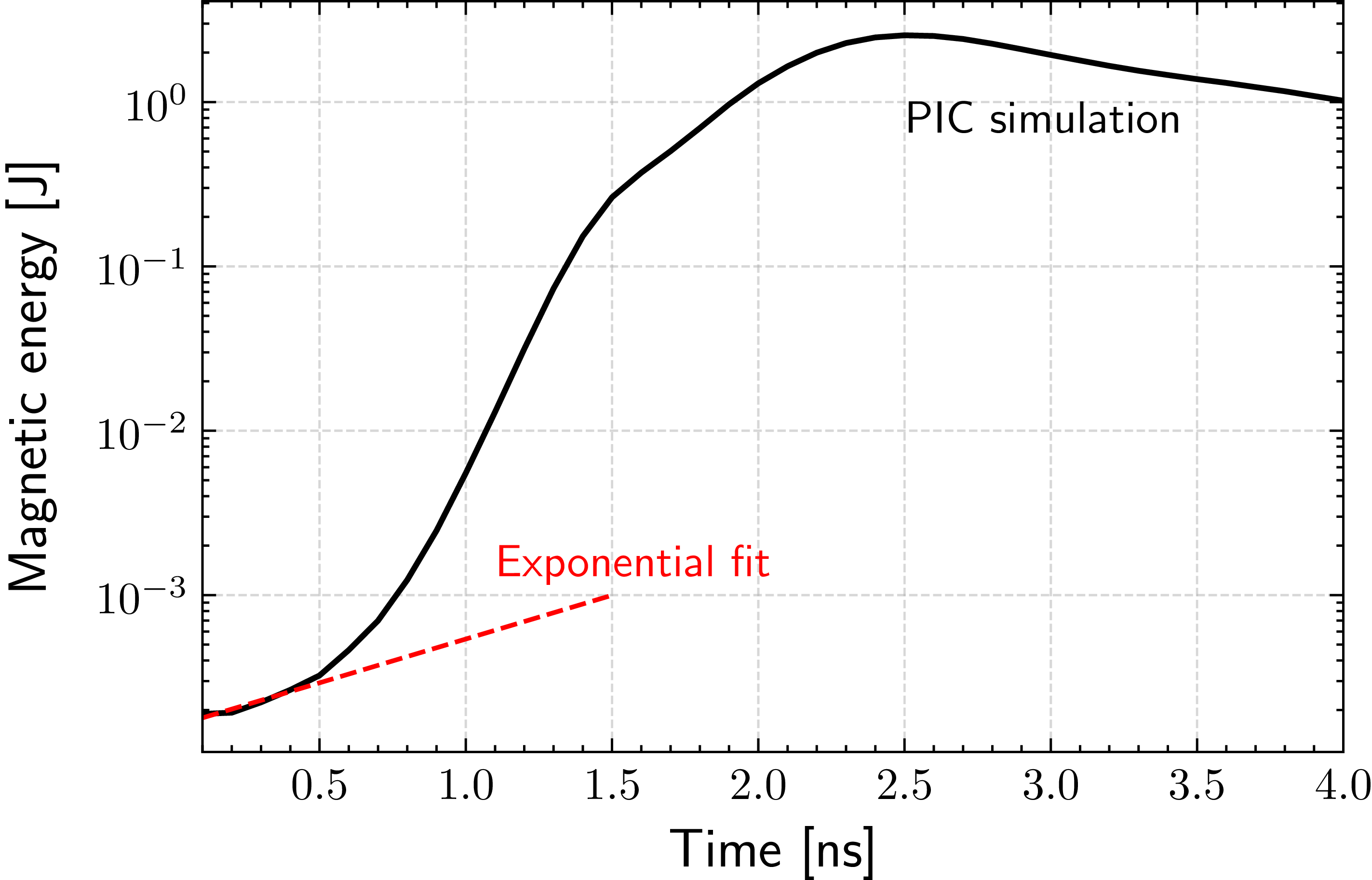
This appendix provides the PIC results for the electron–electron interactions, assuming an idealised bi-Maxwellian distribution described by (3.6). The simulation geometry and resolutions are identical to those described in § 4. Figure 16 depicts the temporal evolution of the magnetic energy, where the initial e-folding time is
 ${\sim} 1.6 \pm 0.3 \, \mathrm{ns}$
. This is in reasonable agreement with theoretical predictions (
 ${\sim} 3 \, \mathrm{ns}$
) made in § 3. Linear theory provides only an approximate solution to the dispersion relation.
Temporal evolution of the magnetic field energy obtained from PIC simulation, using the idealised bi-Maxwellian distribution shown in (3.6). The dotted red line shows the exponential fit to obtain the initial magnetic field growth time of
 $1.6\pm 0.3 \, \mathrm{ns}$
.

Appendix C
This appendix derives the scaling
 $n_e \propto E_L^{0.6}$
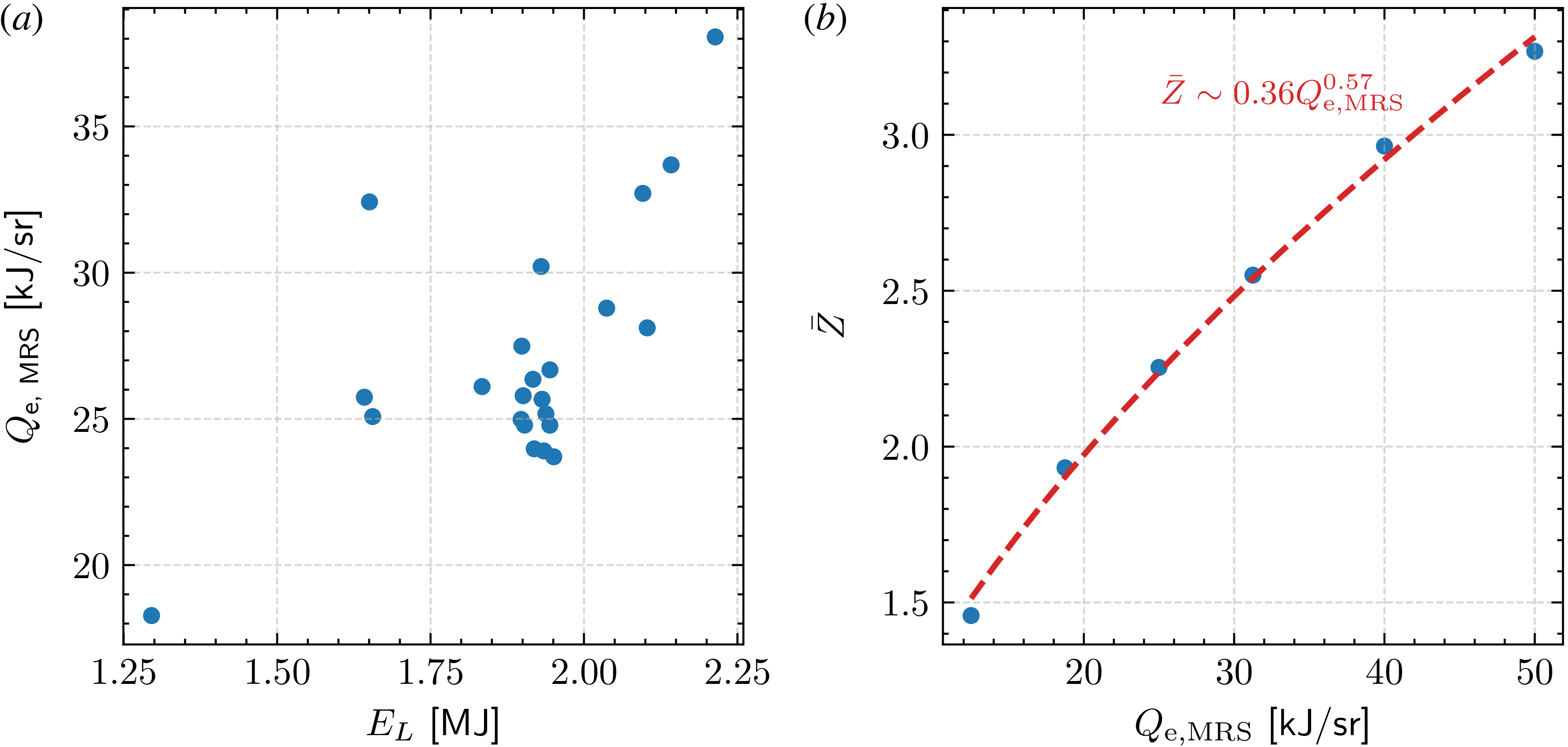
mentioned in § 6. The NIF experiments with available MRS, Dante-2 and vacuum pressure data are considered. For each shot, the radiant energy per solid angle directed towards the MRS,
 $Q_{\text{e, MRS}}$
, is calculated using the energy deposition model described in § 2.3. As shown in figure 17(a),
 $Q_{\text{e, MRS}}$
scales approximately linearly with
 $E_L$
. To connect this to the electron density
 $n_e$
, the average ionisation state
 $\bar {Z}$
is obtained as a function of
 $Q_{\text{e, MRS}}$
by equating (2.5) and (2.6). Here,
 $\sigma _{\text{vac}}$
and
 $f(E_\gamma )$
are assumed constant as they do not vary significantly between shots. As seen in figure 17(b),
 $\bar {Z} \propto Q_{\text{e, MRS}}^{0.6}$
, which combined with the linear scaling in figure 17(a) gives
 $n_e \propto E_L^{0.6}$
.
(a) Experimental scaling of inferred X-ray energy per unit solid angle (towards the MRS) with total laser energy. Scatter points represent NIF experiments for which MRS, Dante-2 and vacuum pressure data are available. (b) Estimated
 $\bar {Z}$
for various
 $Q_{\text{e, MRS}}$
based on the energy-deposition model in § 2.3. The dashed red line shows the power-law best-fit
 $\bar {Z} \sim Q_{\text{e, MRS}}^{0.6}$
.


 θlab
 θlab∼0
 μ
 2
 ≲0.1%

 t∼8
 Z¯>1
 Z¯<1
 r=26
 r=596
 Z¯=7

 vr
 v⊥
 vr
 v⊥

 Bz(r,y)
 t=0
 Bz(r,y)=0
 ∼10cm×10cm
 0.50±0.05ns


 (Yn,ρR,Ti)
 τBW


 y

 t∼60
 t=0
 ΔYn/Yn⩽5.5%
 ΔρR/ρR∼5%
 ΔTi∼0.46
 Yn∼1017
 ρR∼500mgcm−2
 Ti∼10
 EL∼2
 (56.7μm,0.5cm2)
 ρR
 (56.7μm,0.5cm2)
 Yn∼1018
 Ti∼15
 1.6±0.3ns
 Z¯
 Qe, MRS
 Z¯∼Qe, MRS0.6

 Open access

